1. Introduction
Perhaps the most familiar configuration of two-phase flow is that of a gas phase on top of a liquid phase, particularly air and water. The large density ratio means that at rest, gravity keeps the two separated at a flat free surface, with surface tension also playing a role. Sufficiently energetic flows can overcome these forces and distort the free surface to the point where it breaks apart forming bubbles (volumes of air surrounded by water) and drops (volumes of water surrounded by air) (Brocchini & Peregrine Reference Brocchini and Peregrine2001). While drops are also of interest, e.g. in ocean spray (Veron Reference Veron2015), our focus here is on the creation of bubbles, referred to as air entrainment. Air entraining flows, identifiable by the white appearance of the surface, are present in many different natural and engineering contexts. Among the properties of air-entertaining flows, the bubble size distribution is of special interest.
One common air-entraining flow is a breaking wave, where the bubble size distribution has significant implications for air–sea gas exchange due to the ratio of surface area to volume (Thorpe Reference Thorpe1982; Wallace & Wirick Reference Wallace and Wirick1992; Farmer, McNeil & Johnson Reference Farmer, McNeil and Johnson1993; Melville Reference Melville1996) as well as ocean acoustics due to size-dependent acoustic properties (Medwin & Beaky Reference Medwin and Beaky1989; Lamarre & Melville Reference Lamarre and Melville1991; Deane, Preisig & Lavery Reference Deane, Preisig and Lavery2013). Beneath a plunging breaking wave, it is well established that the size distribution of bubbles larger than the Hinze scale, where surface tension is negligible compared to turbulence (Hinze Reference Hinze1955), follows a
 $-10/3$
power law with bubble radius (Deane & Stokes Reference Deane and Stokes2002). This power law can be obtained from first principles under the assumption that the effect of bubble fragmentation by turbulence on the population is dominant over any other physical mechanism (Garrett, Li & Farmer Reference Garrett, Li and Farmer2000). While wide agreement on the
 $-10/3$
power law for plunging breaking waves implies that this model is appropriate there (Deike Reference Deike2022), recent observations of different large-bubble power laws in simulations of the wake behind a vessel (Hendrickson et al. Reference Hendrickson, Weymouth, Yu and Yue2019) and a canonical shear-driven flow (Gaylo, Hendrickson & Yue Reference Gaylo, Hendrickson and Yue2024) highlight that it is not a universal description of bubble populations in air-entraining flows.
For the development of more general models of bubble populations that consider all the relevant physical mechanisms in air-entraining flow, an immediate challenge is that entrainment itself is one of the least understood classes of bubble evolution mechanisms. Different air-entraining flows may have certain specific entrainment mechanisms driven by the large-scale flow structure, e.g. the entrapment of a cavity by a plunging breaking wave (Deike, Melville & Popinet Reference Deike, Melville and Popinet2016; Chan et al. Reference Chan, Johnson, Moin and Urzay2021b ; Gao et al. Reference Gao, Deane and Shen2021b ) or entrainment by a plunging jet (Kiger & Duncan Reference Kiger and Duncan2012; Bertola, Wang & Chanson Reference Bertola, Wang and Chanson2018). More generally, Brocchini & Peregrine (Reference Brocchini and Peregrine2001) note that a common feature of air-entraining flows is strong turbulence beneath the free surface, e.g. spilling breakers, hydrologic jumps, upwelling of existing bubble populations, and flows in steep rivers or spillways. Motivated by this potential broad applicability, this work seeks to characterise the mechanism of air entrainment by this strong free-surface turbulence (FST).
One flow where FST entrainment is relevant is open channel flow, often studied in the context of hydraulic modelling of rivers and spillways (Falvey & Ervine Reference Falvey and Ervine1988; Chanson Reference Chanson1996). Along a spillway, the turbulent boundary layer grows until it reaches the free surface. If the turbulence is sufficiently strong, then the free surface becomes highly distorted, and the flow becomes air-entraining (also known as self-aerating) (Keller, Lai & Wood Reference Keller, Lai and Wood1974; Wilhelms & Gulliver Reference Wilhelms and Gulliver2005). The quantity and size of bubbles are needed to predict how the dissolved-oxygen content changes due to rapids or spillways (Gulliver & Rindels Reference Gulliver and Rindels1993), so a model of bubble entrainment is needed. While some previous work considered bubble formation by the impact of droplets at the free surface, this mechanism is not believed to be energetic enough to explain observed bubbles (Rein Reference Rein1998). Wei et al. (Reference Wei, Xu, Deng, Tian and Zhang2019) use high-speed photography to obtain time series of individual entrainment events. Their direct measurement of individual entrainment events is unlike the more typical approach of measuring the entire resulting bubble population – examples from breaking waves (Deane & Stokes Reference Deane and Stokes2002) and channel flow (Chanson & Toombes Reference Chanson and Toombes2003). This gave Wei et al. (Reference Wei, Xu, Deng, Tian and Zhang2019) new insight into the exact mechanism for entrainment, and they show that entrainment in an open channel is the direct result of the interaction of turbulence with the free surface. That work shows that FST entrainment is relevant to channel flow, and provides what the authors believe to be the first direct experimental measurement of entrainment by FST.
An inherent challenge in direct experimental measurement of FST air entrainment is that the free surface is strongly distorted, making visual access difficult. In total, Wei et al. (Reference Wei, Xu, Deng, Tian and Zhang2019) were able to observe only 108 entrainment events, which is insufficient to obtain detailed statistics, particularly how entrainment scales with bubble size and turbulence strength. For this purpose, direct numerical simulations (DNS) are useful, as all features of the flow are immediately accessible. Recently, there have been advances in bubble tracking (Chan et al. Reference Chan, Dodd, Johnson and Moin2021a
; Gao et al. Reference Gao, Deane, Liu and Shen2021a
; Gaylo, Hendrickson & Yue Reference Gaylo, Hendrickson and Yue2022), which have made it possible to accurately identify and measure individual entrainment events within DNS of complex bubbly flow. In this work, we perform DNS of a canonical flow that isolates entrainment by FST from other entrainment mechanisms, and use the new bubble tracking capability to obtain a large
 ${O}(10^4)$
data set of FST entrainment events.
Based on the direct measurement of entrainment events in DNS, we can elucidate the scaling of the size distribution of FST entrainment with the strength of turbulence and gravity. This observed scaling is explained and supported by a simple mechanistic model. Although our results are based on a flow where FST is the only entrainment mechanism, we show that the same scaling closely describes entrainment size distributions observed in other, more complex free-surface flows where additional entrainment mechanisms are also present.
2. Characterising air entrainment by FST
For bubbly flow, the size distribution of bubbles is of special interest. This size distribution
 $N(a)$
is defined such that
 $N(a)\,\delta a$
is defined as the number of bubbles of (effective) radius
 $[a,a+\delta a]$
in a region of interest. The evolution of
 $N(a)$
is described by a population balance equation
 \begin{equation} \partial N (a)/ \partial t = S_f(a) + S_c(a) + I(a) - D(a) {,} \end{equation}
where each term on the right describes a physical mechanism: fragmentation
 $S_f(a)$
, coalescence
 $S_c(a)$
, entrainment
 $I(a)$
, and degassing
 $D(a)$
. In entraining flows, all right-hand-side terms could have some impact on
 $N(a)$
, which also makes it difficult to infer any single right-hand-side term from
 $N(a)$
alone. In this paper, we consider the entrainment size distribution
 $I(a)$
, where
 $I(a)\,\delta a\, \delta t$
is defined to be the number of bubbles of (effective) radius
 $[a,a+\delta a]$
created at the free surface over time
 $[t, t+\delta t]$
for the region of interest. An entraining free surface can be thought of as a locally flat surface plus perturbations by turbulence, in which case it is natural to normalise
 $I(a)$
by
 $A_{\textit{FS}}$
, the area of the mean free surface in the region of interest. In § 2.1, we perform dimensional analysis to obtain, given some basic properties of strong FST, the set of possible scalings of
 $I(a)/A_{\textit{FS}}$
. In § 2.2, we describe a mechanistic model of FST entrainment that elucidates the scaling. In § 3.3, this scaling is confirmed by direct measurement of
 $I(a)/A_{\textit{FS}}$
in DNS.
2.1. Dimensional analysis
A critical parameter for FST is the strength of the near-surface turbulence relative to the restoring force of gravity, described by a turbulent Froude number (squared):
 \begin{equation} {\textit{Fr}}_T^{\kern1pt 2} = \varepsilon /u_{\textit{rms}} g{,} \end{equation}
where
 $g$
is gravitational acceleration, and the strength of the near-surface turbulence is described by the dissipation rate
 $\varepsilon$
and the root mean velocity fluctuations
 $u_{\textit{rms}}$
. For sufficiently large
 ${\textit{Fr}}_T^{\kern1pt 2}$
, we expect that the free surface will not significantly constrain vertical fluctuations, and the near-surface turbulence will be nearly isotropic and follow the Kolmogorov
 $-5/3$
scaling (Yu et al. Reference Yu, Hendrickson, Campbell and Yue2019). In § 3.2, we show that this is true, and show the range of
 ${\textit{Fr}}_T^{\kern1pt 2}$
where isotropy is obtained. We refer to this regime as strong FST. Thus for strong FST, we can model the turbulence as isotropic such that within the inertial sub-range, the strength of turbulence is fully characterised by
 $\varepsilon =[L^2 T^{-3}]$
. After normalising by the density of water
 $\rho _w$
, the energy to entrain a bubble of radius
 $a = [L]$
is characterised by gravitational acceleration
 $g = [L T^{-2}]$
and surface tension
 $(\sigma /\rho _w) = [L^3 T^{-2}]$
. We will assume that constitutive property ratios, such as the density ratio
 $\rho _a/\rho _w$
and the viscosity ratio
 $\mu _a/\mu _w$
, are fixed for air and water. This gives that
 $I(a)/A_{\textit{FS}}$
(dimensions
 $[L^{-3} T^{-1}]$
) is a function of only
 $\varepsilon$
,
 $a$
,
 $g$
and
 $\sigma /\rho _w$
.
From dimensional analysis, the problem is described by three dimensionless parameters. We choose one parameter to be a Bond number
 ${\textit{Bo}} \equiv g (2 a)^2 / (\sigma /\rho _w)$
, which is the ratio of gravitational to surface energy needed to form a bubble. The critical value
 ${\textit{Bo}}=1$
corresponds to the capillary scale
 \begin{equation} a_c \equiv 0.5 \sqrt {\sigma /g \rho _w}{,} \end{equation}
which gives
 $a_c\approx 1.3$
mm for air–water flows on Earth. For large bubbles with radii
 $a\gg a_c$
(i.e.
 ${\textit{Bo}}\gg 1$
), we expect the effects of surface tension on entrainment to be negligible, so we drop
 ${\textit{Bo}}$
as a parameter. Far from critical values of
 ${\textit{Bo}}$
or
 ${\textit{Fr}}_T^{\kern1pt 2}$
, we assume that the underlying mechanisms are scale-invariant. This assumption implies that the remaining two dimensionless parameters, say
 $\varPi _1$
and
 $\varPi _2$
, are related by a power law
 $\varPi _1 = C_I {\varPi _2}^{\alpha }$
, where
 $\alpha$
describes the scaling, and
 $C_I$
is a scaling constant. Thus dimensional consistency and scale invariance give
 \begin{equation} I(a) \!/\! A_{\textit{FS}} = C_I \, g^{[-\alpha /2 ]}\, \varepsilon ^{[\alpha /3 + 1/3]}\, (2 a)^{[-\alpha /6 - 11/3]} \quad \text{for }a\gg a_c{,} \end{equation}
where
 $\alpha$
and
 $C_I$
are to be determined.
For FST, it is useful to normalise by near-surface turbulence scales
 $L_T=u_{\textit{rms}}^3/\varepsilon$
and
 $T_T=u_{\textit{rms}}^2/\varepsilon$
. Thus (2.4) can be non-dimensionalised:
 \begin{equation} [ I(a)\!/\! A_{\textit{FS}} ]^* = C_I \; \left ({\textit{Fr}}_T\right )^{[\alpha ]} \; (2 a^* )^{[-\alpha /6 - 11/3]} \quad \text{for }Bo\gg 1{,} \end{equation}
where the non-dimensionalised bubble radius is
 $a^*\equiv a/L_T$
, and the non-dimensionalised entrainment size distribution is
 $[I(a)/A_{\textit{FS}}]^*\equiv [I(a)/A_{\textit{FS}}] {L_T}^3 T_T$
. In this non-dimensional form, it is clear that the value
 $\alpha$
describes how large-bubble air entrainment by FST scales with turbulent Froude number.
2.2. A model for large-bubble air entrainment by FST
We now propose a mechanistic model of entrainment that obtains the value of
 $\alpha$
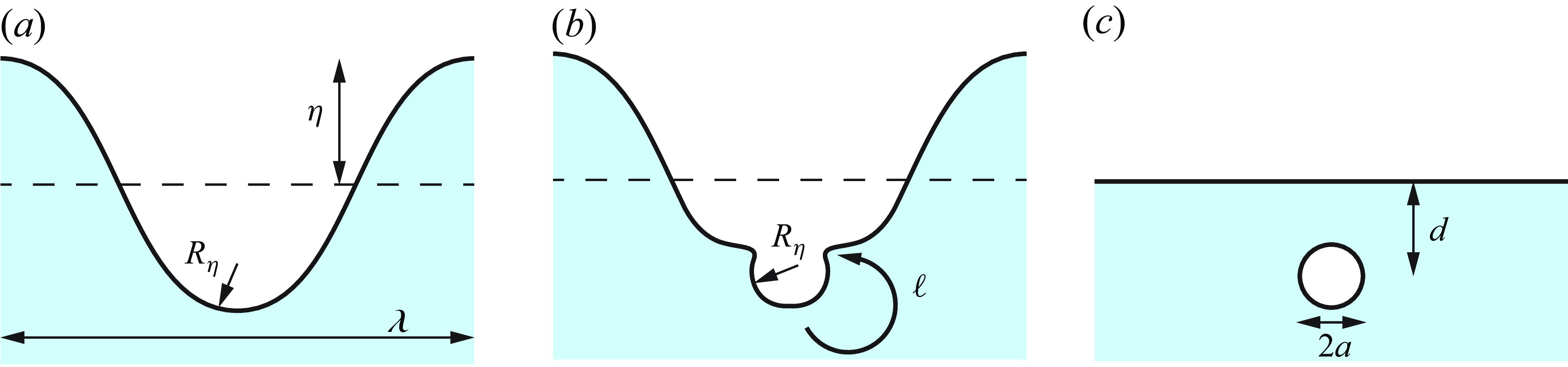
and predicts the scaling that we observe in DNS (see § 3.3). As a simplified model, we consider three stages for entrainment, illustrated in figure 1. First, there is a free-surface deformation of wavelength
 $\lambda$
, height
 $\eta$
, with a minimum radius of curvature
 $R_\eta$
caused by FST. Second, interaction with a turbulent eddy causes the deformation to collapse. Finally, a single bubble of radius
 $a$
is entrained. Central to our mechanistic model is that during the collapse of the surface, the minimum radius does not change significantly, such that the radius
 $a$
of the bubble formed scales with the minimum radius of curvature
 $R_\eta$
of the initial surface deformation, i.e.
 $a\sim R_\eta$
. This insight is consistent with observation by Wei et al. (Reference Wei, Xu, Deng, Tian and Zhang2019) that as air-entraining surface deformations collapse, the minimum radius of curvature approaches an asymptotic value
 $r_c$
that increases with the size of bubble eventually obtained, and is consistent with our qualitative observations from DNS (figure 2). In this subsection, we apply an energy balance argument to derive
 $I(a)$
based on this model.
Illustration of three stages of air entrainment. (a) A free-surface deformation exists with amplitude
 $\eta$
, wavelength
 $\lambda$
, and minimum radius of curvature
 $R_\eta$
. (b) It interacts with an eddy of size
 $\ell$
. (c) A bubble of radius
 $a\sim R_\eta$
is formed at depth
 $d$
.

Three examples of air-entrainment events, viewed from below the free surface, taken from a DNS simulation (b.ii) described in § 3. Each frame is
 $62\ \mathrm{mm}\times 62\ \mathrm{mm}$
and separated in time by
 $17\ \mathrm{ms}$
. A large surface deformation collapses into a single bubble (highlighted in yellow for (b) and (c)). The minimum radius of curvature does not change significantly, leading to
 $a\sim R_\eta$
.

We first seek an expression for
 $R_\eta$
as a function of the deformation wavenumber
 $\kappa = 2 \unicode{x03C0} /\lambda$
. As confirmed in § 3.2, near-surface turbulence is isotropic at sufficiently large
 ${\textit{Fr}}_T$
, allowing application of the Kolmogorov energy cascade (Yu et al. Reference Yu, Hendrickson, Campbell and Yue2019). Within the inertial range, the power spectrum of pressure fluctuations is given by
 $E_{pp}(\kappa )= 2.97 \, \rho _w^2 \varepsilon ^{4/3} \kappa ^{-7/3}$
(George, Beuther & Arndt Reference George, Beuther and Arndt1984). For
 ${\textit{Bo}}\gg 1$
, such that surface tension is negligible, we use the linearised relationship between pressure fluctuations and surface elevation,
 $p \sim \rho _w g \eta$
, to obtain the surface elevation spectrum:
 \begin{equation} E_{\eta \eta }(\kappa ) \sim 2.97 \, g^{-2} \varepsilon ^{4/3} \kappa ^{-7/3} {.} \end{equation}
After multiplying by
 $\delta \kappa \sim \kappa$
, the characteristic amplitude
 $\eta$
for a surface disturbance of wavenumber
 $\kappa$
is
 \begin{equation} \eta ^2 \propto g^{-2} \varepsilon ^{4/3} \kappa ^{-4/3}{.} \end{equation}
Assuming a sinusoidal disturbance, the minimum radius of curvature is
 $R_\eta = \kappa ^{-2} \eta ^{-1}$
(with a similar scaling for other geometries such as Gaussian; Wei et al. Reference Wei, Xu, Deng, Tian and Zhang2019) such that
 \begin{equation} R_\eta \propto g \, \varepsilon ^{-2/3} \kappa ^{-4/3}{.} \end{equation}
Applying
 $a\sim R_\eta$
and rearranging, we determine the turbulence scales
 $\kappa$
that are responsible (through interaction with the free surface) for generating bubbles of radius
 $a$
:
 \begin{equation} \kappa \propto g^{3/4} \varepsilon ^{-1/2} a^{-3/4}{.} \end{equation}
This is distinct from previous energy-based mechanistic models of air entrainment (Rein Reference Rein1998; Yu, Hendrickson & Yue Reference Yu, Hendrickson and Yue2020), which assume that bubbles of radius
 $a$
are entrained by turbulence eddies of similar scales, i.e.
 $\kappa \sim a^{-1}$
. While this is consistent dimensionally, it does not capture the inter-scale energy transfer that we observe with (2.9).
We now perform an energy balance including this new (2.9) describing inter-scale energy exchange. For a small range of wavenumbers
 $[\kappa , \kappa +\delta \kappa ]$
, the potential energy associated with the surface deformations (per free-surface area
 $A_{\textit{FS}}$
) is
 \begin{equation} {\textit{PE}}_{w\textit{a}v\textit{es}}/\! A_{\textit{FS}} = \rho _w g \, E_{\eta \eta }(\kappa ) \, \delta \kappa {.} \end{equation}
Applying the wave spectrum (2.6),
 \begin{equation} {\textit{PE}}_{w\textit{a}v\textit{es}}/\! A_{\textit{FS}} \propto \rho _w g^{-1} \varepsilon ^{4/3} \kappa ^{-7/3} \, \delta \kappa {.} \end{equation}
For the necessary work done,
 $W_{\textit{ent}}$
, to entrain bubbles of radius
 $[a, a+\delta a]$
, we assume that bubbles are entrained to a depth
 $d\sim 2a$
, as shown in figure 1(c), to obtain (Yu et al. Reference Yu, Hendrickson and Yue2020)
 \begin{equation} W_{\textit{ent}} = I(a) \, \left (8 \unicode{x03C0} /3\right ) \rho _w g a^4 \, \delta a {.} \end{equation}
Figure 1(b) illustrates that for the surface deformation to collapse into a bubble, some perturbation is necessary. We argue that this perturbation will come from eddies of size
 $\ell \sim R_\eta$
(or equivalently
 $\ell \sim a$
), and
 $T_{\textit{ent}}$
is the associated eddy turnover time. From the Kolmogorov energy cascade,
 $T_{\textit{ent}}\sim \varepsilon ^{-1/3} a^{2/3}$
. Finally, we set
 $W_{\textit{ent}} T_{\textit{ent}} = {\textit{PE}}_{\textit{waves}}$
and use (2.9) as well as the derivative
 $\partial \kappa /\partial a$
to solve for
 $I(a)$
in terms of bubble radius:
 \begin{equation} I(a)/A_{\textit{FS}} \propto g^{-3} \varepsilon ^{7/3} a^{-14/3}{.} \end{equation}
This corresponds to
 $\alpha = 6$
in (2.4), or FST entrainment scaling with
 ${\textit{Fr}}_T^6$
in (2.5).
3. Direct numerical simulation of entrainment by FST
To study entrainment by FST, we seek a flow that isolates FST entrainment from any other entrainment mechanism. This is obtained with forced FST, where isotropic turbulence is continuously forced deep beneath the surface to obtain statistically steady turbulence and bubble population at the free surface. The set-up of our simulations is based on Guo & Shen (Reference Guo and Shen2009), but extended to large
 ${\textit{Fr}}$
where entrainment occurs.
3.1. Simulation set-up
We perform DNS by solving the (non-dimensionalised) three-dimensional incompressible Navier–Stokes equation for velocity
 $\boldsymbol{u}$
:
 \begin{align}& \frac {\partial \boldsymbol{u}}{\partial t} + \boldsymbol{\nabla \boldsymbol{\cdot }\left (\boldsymbol{u}\boldsymbol{u}\right )} = - \frac {1}{\rho } \boldsymbol{\nabla }{p} + \frac {1}{\rho {\textit{Re}}} \boldsymbol{\nabla} \boldsymbol{\cdot }\left (2 \mu \boldsymbol{E}\right ) - \frac {\hat {\boldsymbol{e}}_z}{\textit{Fr}^2} +\frac {\kappa \delta _s}{\textit{We}} \hat {\boldsymbol{n}} + \boldsymbol{f}{,} \end{align}
 \begin{align}&\qquad\qquad\qquad\qquad\qquad\qquad \boldsymbol{\nabla \boldsymbol{\cdot }\boldsymbol{u}} = 0{,} \end{align}
where
 $p$
is the pressure field, and the rate-of-strain tensor is
 $\boldsymbol{E} = 1/2 (\boldsymbol{\nabla }{\boldsymbol{u}}+\boldsymbol{\nabla }{\boldsymbol{u}}^{{T}})$
. We do not consider the solubility of air in water, so the two immiscible phases are described by a binary colour function
 $c(\boldsymbol{x},t)$
, where
 $c=1$
in water,
 $c=0$
in air, and
 \begin{equation} \frac {\partial c}{\partial t} + \boldsymbol{u} \boldsymbol{\cdot }\boldsymbol{\nabla }{c} = 0 {.} \end{equation}
(Non-dimensional) density and viscosity are defined as
 $\rho \equiv c + (1-c) \rho _a/\rho _w$
and
 $\mu \equiv c + (1-c) \mu _a/\mu _w$
, where we use realistic air–water values
 $\rho _{a}/\rho _{w}=0.00123$
and
 $\mu _{a}/\mu _{w}=0.0159$
. We solve these equations on a uniform Cartesian grid using a second-order finite volume scheme (Campbell Reference Campbell2014; Yu et al. Reference Yu, Hendrickson, Campbell and Yue2019). Equation (3.1c
) is solved using a volume-of-fluid method, which ensures volume conservation of air and water to machine precision (Weymouth & Yue Reference Weymouth and Yue2010). Surface tension is modelled using the continuous surface force method (Brackbill, Kothe & Zemach Reference Brackbill, Kothe and Zemach1992; Popinet Reference Popinet2009).
Following Guo & Shen (Reference Guo and Shen2009), to maintain isotropic turbulence in a bulk region deep beneath the free surface, we use a linear forcing term
 \begin{equation} \boldsymbol{f} = A \boldsymbol{u}'\, F_b(z_c) {,} \end{equation}
where
 $\boldsymbol{u}'=\boldsymbol{u}-\bar {\boldsymbol{u}}$
is the turbulent component of the velocity (
 $\bar {\boldsymbol{u}}(z,t)$
is from an instantaneous average in each
 $z$
-plane), and
 $A$
is a value chosen dynamically to obtain a target dissipation rate
 $\varepsilon _{0}\approx 1$
in the bulk. The horizontal domain length is chosen to be
 $2 \unicode{x03C0}$
. These lead to an integral length scale in the bulk (
 $L = u_{{\textit{rms},}0}^3/\varepsilon _{0}$
) that is also approximately unity (Rosales & Meneveau 2005). We choose these values to be unity such that the simulation is non-dimensionalised in terms of the characteristic scales of turbulence in the bulk region, e.g.
 ${\textit{Fr}}^2 = \varepsilon _{0}/u_{{\textit{rms},}0}\, {g}$
. The function
 \begin{equation} F_b(z_c) = \begin{cases} 0, & z_c \gt l_b + l_d, \\ \frac {1}{2} \left (1 - \cos {\left [\frac {\unicode{x03C0} }{l_d}(z_c - l_b - l_d)\right ]}\right )\!, & z_c\leqslant l_b + l_d, \\ 1, & z_c \leqslant l_b, \\ \end{cases} \end{equation}
defines the region where forcing is applied, with
 $z_c$
measured from the centre of the bulk region. The bulk region extends over
 $2 l_b = 3 \unicode{x03C0}$
, with a damping region
 $l_d=\unicode{x03C0} /2$
on either side, and then a free length
 $l_f=\unicode{x03C0} /2$
before the bottom of the domain or the free surface at
 $z=0$
. Thus
 $z_c=\lvert z+l_f+l_d+l_b \rvert$
. We add an air-gap region of height
 $\unicode{x03C0}$
above the free surface, to give total domain height
 $6\unicode{x03C0}$
.
For all simulations, we set
 $\textit{Re}=200$
and use a grid
 $256^2 \times 768$
. The DNS require resolution of the Kolmogorov micro scale
 $\eta _T=(\nu ^3/\varepsilon )^{1/4}$
. In the bulk region where turbulence is strongest,
 $\eta _T / \varDelta \approx 0.78$
. Near the free surface, where we are interested,
 $\eta _T / \varDelta \approx 1.8$
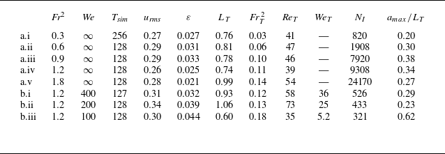
, sufficient for DNS of FST (Yu et al. Reference Yu, Hendrickson, Campbell and Yue2019; Gaylo et al. Reference Gaylo, Hendrickson and Yue2024). To obtain different conditions (see table 1), we change
 ${\textit{Fr}}$
and
 ${\textit{We}}$
in (3.1a
), with
 ${\textit{We}}=\infty$
corresponding to cases where surface tension is not modelled (simulations a.i–a.v). Simulations are initialised from a random velocity in the bulk and a free surface at
 $z=0$
, then run for at least
 $400$
bulk eddy turnover times, while considering total gravitational potential energy, turbulence statistics, bubble population and entrainment statistics to assess convergence to a steady state. After a statistically steady state is reached at
 $t=t_0$
, steady-state statistics are obtained over
 $t\in [t_0, t_0+T_{\textit{sim}}]$
. Figure 3 shows a rendering of the simulation near the free surface.
Summary of DNS, where
 $N_I$
is the number of (resolved) entrainment events recorded, and
 $a_{{max}}$
is the (effective) radius of the largest entrained bubble observed.

Rendering of simulation b.ii showing the free surface and bubbly flow beneath. Scaling to match Earth gravity and air–water surface tension and density, each square on the background grid is
 $1.09\ \mathrm{cm}$
across.

While the simulation set-up allows us to prescribe the turbulence levels in the bulk region, our interest is the turbulence levels near the surface. Guo & Shen (Reference Guo and Shen2009) provide an empirical fit for
 ${\textit{Fr}}^2\ll 1$
; however, the near-surface turbulence is not known a priori. Instead, we measure the near-surface turbulence a posteriori, and calculate new non-dimensional numbers to properly characterise the near-surface turbulence. The FST is driven by turbulence in the water (Brocchini & Peregrine Reference Brocchini and Peregrine2001), so for measurements of turbulence, we consider averages in the water phase where
 $c=1$
. We define a near-surface water-phase average
 \begin{equation} \langle \boldsymbol{\cdot } \rangle _\delta \equiv \frac {\iiiint \boldsymbol{\cdot } \; c \,\mathrm{d} \boldsymbol{x}\, \mathrm{d} t}{\iiiint c \,\mathrm{d} \boldsymbol{x}\, \mathrm{d} t} \quad \text{for } z\gt -\delta \text{ and } t\in [t_0, t_0+T_{\textit{sim}}]{.} \end{equation}
Seeking to match
 $\delta /L_T \approx 0.5$
from previous work (Yu et al. Reference Yu, Hendrickson, Campbell and Yue2019; Gaylo et al. Reference Gaylo, Hendrickson and Yue2024), we choose
 $\delta =0.3$
to define the ‘near surface’. Because of the symmetry and steady-state nature of the flow,
 $\langle \boldsymbol{u} \rangle _\delta \approx \boldsymbol{0}$
and we treat all velocity as turbulent fluctuations. This defines a near-surface
 $u_{\textit{rms}} = \sqrt {\langle \boldsymbol{u} \boldsymbol{\cdot }\boldsymbol{u} \rangle _\delta /3}$
and a dissipation rate
 $\varepsilon = 2 \langle \mu \boldsymbol{E} : \boldsymbol{E} \rangle _\delta /\textit{Re}$
. From these two values, we calculate near-surface turbulent scales
 $L_T=u_{\textit{rms}}^3/\varepsilon$
and
 $T_T=u_{\textit{rms}}^2/\varepsilon$
, as well as the turbulent Froude number
 ${\textit{Fr}}^2_T = Fr^2 \, u_{\textit{rms}}^2/ L_T$
, turbulent Reynolds number
 ${\textit{Re}}_T = {\textit{Re}}\, u_{\textit{rms}} L_T$
, and turbulent Weber number
 ${\textit{We}}_T = \textit{We} \, u_{\textit{rms}}^2 L_T$
. All are shown in table 1. The near-surface turbulence generally scales with the bulk turbulence, e.g.
 ${\textit{Fr}}_T^{\kern1pt 2} \approx 0.1 Fr^2$
and
 $L_T\approx 0.8$
; however, as expected, free surface motion and the presence of bubbles effect the diffusion of turbulence from the bulk to the surface, leading to small deviations in the scaling, especially for larger
 ${\textit{Fr}}^2_T$
and smaller
 ${\textit{We}}_T$
.
3.2. Near-surface turbulence isotropy
A basis of the previous dimensional analysis and mechanistic model of entrainment in § 2 is that at sufficiently large
 ${\textit{Fr}}^2_T$
(strong FST), the near-surface turbulence can be treated as isotropic. Before studying the scaling of FST entrainment, we determine the range of
 ${\textit{Fr}}^2_T$
where this is true.
The isotropy parameter
 $J$
for a range of
 ${\textit{Fr}}_T^{\kern1pt 2}$
and negligible surface tension. To the right, solid lines show vertical fluctuations
 $\langle ww \rangle$
and dashed lines show horizontal fluctuations
 $\langle uu \rangle$
for
 ${\textit{Fr}}_T^{\kern1pt 2}=0.03$
,
 $0.06$
and
 $0.11$
. Here,
 ${\textit{Fr}}_T^{\kern1pt 2}=0.11$
is representative of all
 ${\textit{Fr}}_T^{\kern1pt 2} \geqslant 0.1$
.

A simple measure of isotropy is to compare vertical fluctuations
 $\langle ww \rangle$
to horizontal fluctuations
 $\langle uu \rangle$
, using water-phase averages as a function of depth
 $z$
:
 \begin{equation} \langle \boldsymbol{\cdot } \rangle \equiv \frac {\iiint \boldsymbol{\cdot } \; c \,\mathrm{d} x \,\mathrm{d}y\, \mathrm{d} t}{\iiint c \,\mathrm{d} x\, \mathrm{d} y \,\mathrm{d} t} \quad \text{for } t\in [t_0, t_0+T_{\textit{sim}}]{.} \end{equation}
More formally, one can start with the anisotropy tensor
 $b_{\textit{ij}}\equiv \langle u_i u_j \rangle /\langle u_k u_k \rangle - \delta _{\textit{ij}}/3$
, and consider the turbulent isotropy parameter
 \begin{equation} J \equiv 1 - 9 \left (\frac {1}{2} b_{\textit{ij}} b_{\textit{ij}} - b_{\textit{ij}} b_{jk} b_{ki} \right )\!{,} \end{equation}
where
 $J\in [0,1]$
, and
 $J=1$
corresponds to isotropic turbulence (Pope Reference Pope2000). Both measures are shown in figure 4.
For weak FST, the free surface constrains vertical fluctuations, and in the limit
 ${\textit{Fr}}_T\to 0$
, we expect
 $\langle ww \rangle =0$
and
 $J=0$
at the free surface (Hunt & Graham Reference Hunt and Graham1978; Shen et al. Reference Shen, Zhang, Yue and Triantafyllou1999). However, it has been shown that for strong FST (large
 ${\textit{Fr}}_T$
), this boundary effect weakens and the turbulence becomes nearly isotropic (Yu et al. Reference Yu, Hendrickson, Campbell and Yue2019). For
 ${\textit{Fr}}^2_T\geqslant 0.1$
, we observe nearly isotropic turbulence,
 $\langle ww \rangle \approx \langle uu \rangle$
and
 $J\approx 0.95$
, as expected for strong FST. For
 ${\textit{Fr}}_T^{\kern1pt 2}\lt 0.1$
, we see a moderate FST regime where the turbulence becomes more anisotropic as
 ${\textit{Fr}}_T$
decreases, although
 $J$
is still far from
 $J\approx 0$
, characteristic of weak FST. This shows that the isotropic turbulence assumption in § 2.1 is valid for
 ${\textit{Fr}}_T^{\kern1pt 2}\geqslant 0.1$
, and may approximately hold for
 ${\textit{Fr}}_T^{\kern1pt 2}\lesssim 0.1$
.
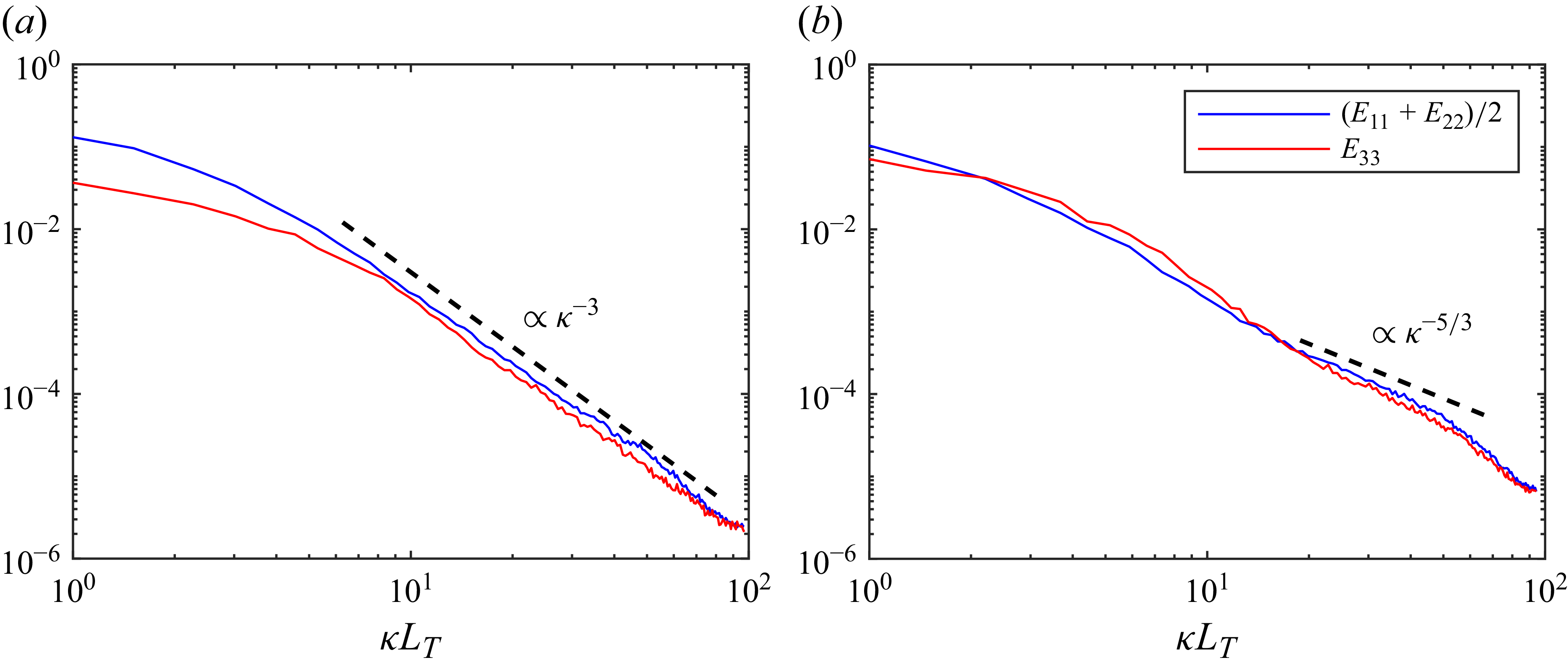
One-dimensional turbulent energy spectra at
 $z=0$
for (a) moderate FST (
 ${\textit{Fr}}_T^{\kern1pt 2}=0.03$
), and (b) strong FST (
 ${\textit{Fr}}_T^{\kern1pt 2}=0.11$
). As
 $E_{11}\approx E_{22}$
, for clarity the horizontal components are averaged.

In addition to measuring isotropy, we examine the turbulence energy spectrum at
 $z=0$
. From the momentum
 $\boldsymbol{p} \equiv \rho \boldsymbol{u}$
measured at
 $z=0$
, we apply Fourier analysis and average over
 $t\in [t_0, t_0+T_{\textit{sim}}]$
to obtain the one-dimensional (in the
 $x$
-direction) energy spectrum
 $E_{\textit{ii}}$
, normalised such that
 $\int (E_{11} + E_{22} + E_{33} )\, \mathrm{d} \kappa =1$
. Figure 5 compares the spectra of moderate and strong FST. For moderate FST, we see that the horizontal fluctuations are stronger than the vertical fluctuations at all scales, and that
 $E\propto \kappa ^{-3}$
, characteristic of two-dimensional turbulence (Kraichnan Reference Kraichnan1967). For strong FST, we see that the turbulence is isotropic at all scales (i.e.
 $E_{11}\approx E_{22}\approx E_{33}$
for all
 $\kappa$
), and that there is a range of
 $\kappa$
where
 $E\propto \kappa ^{-5/3}$
, consistent with the inertial sub-range of isotropic turbulence.
3.3. Entrainment size distribution
Our interest is the entrainment size distribution
 $I(a)$
, which can be obtained directly using the Eulerian label advection (ELA) method (Gaylo et al. Reference Gaylo, Hendrickson and Yue2022, Reference Gaylo, Hendrickson and Yue2024). For completeness and illustration of the application of ELA to obtain
 $I(a)$
in this context, here we provide a summary of the approach. The ELA method identifies individual entrainment events during
 $t\in [t_0, t_0+T_{\textit{sim}}]$
, from which
 $I(a)$
can be calculated. Because bubbles in these simulations undergo other processes, such as degassing and fragmentation,
 $I(a)$
cannot be reliably inferred from
 $\partial N(a)/\partial t$
through (2.1). Instead, the ELA method adds an additional advection equation to the fluid solver,
 \begin{equation} \frac {\partial \boldsymbol{c}^{n}}{\partial t} + \boldsymbol{u} \boldsymbol{\cdot }\boldsymbol{\nabla }{\boldsymbol{c}^n} = 0, \end{equation}
where
 $\boldsymbol{c}^n$
is a vector defined such that
 $c^n_\ell (\boldsymbol{x},t^n)=1$
for
 $\boldsymbol{x} \in$
air that was in a contiguous region of air labelled
 $\ell$
at the snapshot in time
 $t^n$
, and zero otherwise. Numerically, identification of contiguous regions of air is done using interface normals (Hendrickson, Weymouth & Yue Reference Hendrickson, Weymouth and Yue2020), and the ELA method provides a computationally efficient volume-conservative to machine precision way to solve (3.7). By evolving
 $\boldsymbol{c}^n$
to a later snapshot in time
 $t^{n+1}=t^{n}+T_s$
, we obtain
 $\boldsymbol{c}^n(\boldsymbol{x},t^{n+1})$
, which describes the source of air at
 $t^{n+1}$
in terms of the contiguous regions of air previously identified at
 $t^{n}$
. Because the ELA method is volume-conservative,
 $\boldsymbol{c}^n(\boldsymbol{x},t^{n+1})$
describes the source of all air in the domain.
After obtaining
 $\boldsymbol{c}^n(\boldsymbol{x},t^{n+1})$
using ELA, we identify the new set of contiguous regions of air at time
 $t^{n+1}$
. The evolution of bubbles over the snapshot interval
 $t^n$
to
 $t^{n+1}$
can be described in terms of a volume tracking matrix, where each element
 \begin{equation} q_{\textit{ij}} \equiv \int _{\boldsymbol{x}\in {bubble}\ i} c^n_j\big(\boldsymbol{x},t^{n+1}\big)\, \mathrm{d} V \end{equation}
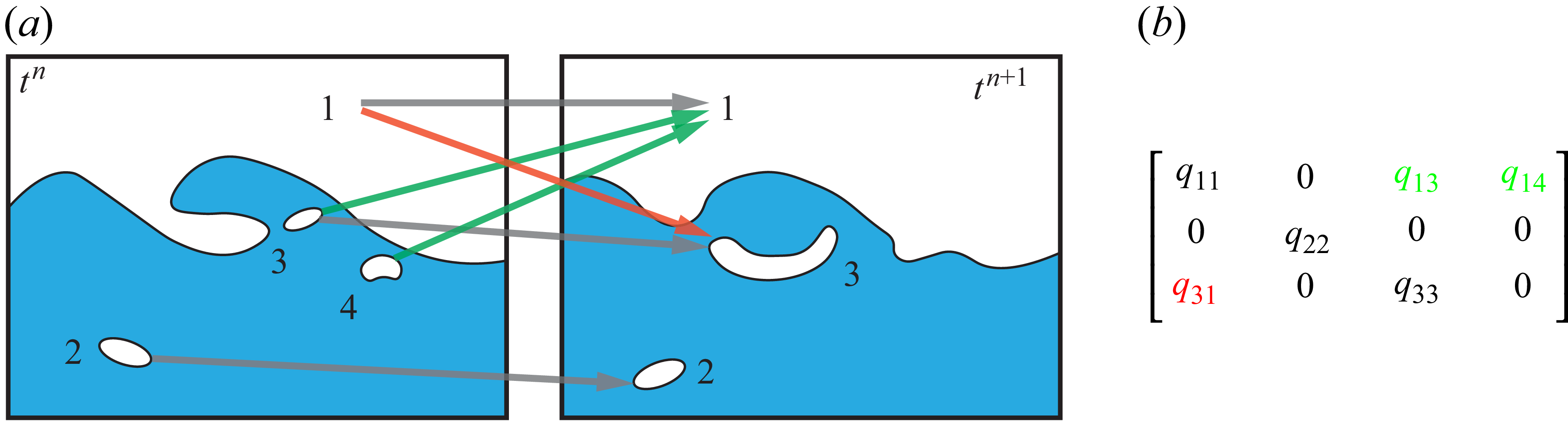
(a) Illustration of entrainment (red) and degassing (green). (b) The associated volume tracking matrix. At
 $t^{n}$
, there is
 $j=1$
and three bubbles
 $j=2,3,4$
. At
 $t^{n+1}$
, there is
 $i=1$
and two bubbles
 $i=2,3$
. Reprinted from Gaylo et al. (Reference Gaylo, Hendrickson and Yue2024).

gives the volume of air from a bubble
 $j$
at time
 $t^{n}$
that contributes to a bubble
 $i$
at time
 $t^{n+1}$
. Gaylo et al. (Reference Gaylo, Hendrickson and Yue2024) describe how the volume tracking matrix given by (3.8) can be used to measure entrainment and degassing, illustrated in figure 6. First, we determine the labels that correspond to the bulk air above the free surface (the ‘sky’) at
 $t^{n}$
and at
 $t^{n+1}$
. For illustration, figure 6 shows the ‘sky’ labelled
 $1$
at both times. Excluding
 $q_{11}$
, which represents air that stayed in the ‘sky’, each non-zero entry in the column
 $q_{i 1}$
represent an individual entrainment event, with the entrained volume
 $v = q_{i 1}$
. In this way, we obtain direct measurement of entrainment events over the snapshot interval
 $T_s$
. We choose
 $T_s=0.16$
to give a similar value of
 $T_s/T_T$
as Gaylo et al. (Reference Gaylo, Hendrickson and Yue2024), who found their measurement of terms in (2.1), including
 $I(a)$
, to be independent of
 $T_s$
.
For each individual entrainment event, we calculate the effective radius in terms of the entrained volume
 $v$
,
 $a \equiv (3 v/4 \unicode{x03C0} )^{1/3}$
. To ensure that the relevant physics is resolved by the numerical grid, we only report bubbles
 $a\gt a_{\textit{res}}$
, where
 $a_{\textit{res}}=1.5 \varDelta$
for simulations where surface tension is not modelled (Yu et al. Reference Yu, Hendrickson, Campbell and Yue2019; Gaylo et al. Reference Gaylo, Hendrickson and Yue2024), and
 $a_{\textit{res}}=3.5 \varDelta$
for simulations where surface tension is modelled (Yu et al. Reference Yu, Hendrickson and Yue2020). The total number of resolved entrainment events
 $N_I$
, as well as the largest single entrained bubble
 $a_{{max}}$
, are shown in table 1. We bin the entrainment events by radius. Starting with
 $\sqrt {N_I}$
bins evenly spaced over
 $\log (a)$
, we combine bins until there are at least
 $15$
events per bin. Normalising by the width of each bin,
 $T_{sim}$
, and
 $A_{\textit{FS}}=4 \unicode{x03C0} ^2$
gives
 $I(a)/A_{\textit{FS}}$
.
Entrainment size distribution (a) as measured and (b) normalised by
 ${\textit{Fr}}_T^6$
for different turbulent Froude numbers
 ${\textit{Fr}}_T= \sqrt {\varepsilon / u_{\textit{rms}} g}$
. In (b), the dashed line shows (2.5) with
 $\alpha =6$
and
 $C_I=3.62$
(
 $R^2=0.990$
excluding
 ${\textit{Fr}}_T^{\kern1pt 2}=0.03$
). Recall that
 $a^*= a\, \varepsilon \, u_{\textit{rms}}^{-3}$
and
 $[I(a)/A_{\textit{FS}}]^*= [I(a)/A_{\textit{FS}}]\, u_{\textit{rms}}^{11}\, \varepsilon ^{-4}$
.

Figure 7 shows the entrainment size distribution for simulations without surface tension (simulations a.i–a.v in table 1). We first perform regression to obtain
 $\alpha$
and
 $C_I$
. Because (2.5) is based on the assumption of isotropic near-surface turbulence, we initially consider the results from only the three
 ${\textit{Fr}}_T^{\kern1pt 2}\geqslant 0.1$
simulations. Least squares regression in
 $\log$
-
 $\log$
space (after binning,
 $n=226$
) gives
 $95\%$
confidence intervals
 $\alpha \in [5.6,6.1]$
and
 $C_I\in [2.65, 3.87]$
. The mechanistic model that we derive in § 2.2 gives
 $\alpha =6$
, consistent with the regression, and if we fix
 $\alpha =6$
, then the regression gives the
 $95\,\%$
confidence interval
 $C_I=3.62\pm 0.10$
. Figure 7(b) shows the collapse of the entrainment size distribution when normalised by
 ${\textit{Fr}}^6_T$
for all but the lowest
 ${\textit{Fr}}_T^{\kern1pt 2}=0.03$
, where the turbulence deviates furthest from isotropy. Even including
 ${\textit{Fr}}_T^{\kern1pt 2}=0.06$
, where turbulence is weakly anisotropic, our model shows a strong agreement (
 $R^2=0.990$
) with the numerical results.
The strong observed correlation with DNS confirms that (2.4) describes the scaling of FST entrainment for large bubbles (
 $a\gg a_c$
) where surface tension is negligible. These results also show that
 $\alpha =6$
, so, consistent with (2.13) derived from our mechanistic model, we have
 \begin{equation} I(a) / A_{\textit{FS}} = C_I \, g^{-3}\, \varepsilon ^{7/3}\, \left (2 a\right )^{-14/3} \quad \text{for }a\gg a_c{,} \end{equation}
where
 $C_I\approx 3.62$
for this limiting case of negligible surface tension. This distribution applies for bubbles as large as
 $a_{{max}} \approx 0.3 L_T$
, above which there is no entrainment (see table 1). For our model of entrainment by FST in § 2.2, (2.9) implies a Froude-sensitive limit on the ratio between
 $a_{max}$
and
 $L_T$
(which sets the smallest value of
 $\kappa$
); however, entrainment also requires interaction with an eddy similar in size to the bubble. The similar values of
 $a_{max}/L_T$
across
 ${\textit{Fr}}_T^{\kern1pt 2}$
suggest that interaction with a similar-sized eddy is the cause of the limit on the largest entrained bubble size in FST.
3.4. Effect of weak surface tension
So far, we have considered the limiting case of negligible surface tension. We now consider the effects of finite surface tension on FST entrainment. The turbulent Weber number,
 \begin{equation} \textit{We}_T \equiv u_{\textit{rms}}^5 / \varepsilon (\sigma /\rho _w), \end{equation}
characterises the strength of near-surface turbulence relative to surface tension. Holding
 ${\textit{Fr}}^2_T\approx 0.11$
constant, we perform DNS of three different
 ${\textit{We}}_T\gg 1$
within the strong FST regime (nearly-isotropic near-surface turbulence). While the computational limits of DNS prevent us from directly matching viscosity, for each
 ${\textit{We}}_T$
we can match
 $\sigma =72\ \mathrm{mN}\ \mathrm{m}^{-1}$
,
 $\rho _w= 1024 \ \mathrm{kg}\ \mathrm{m}^-{^3}$
and
 $g= 9.81 \ \mathrm{m}\ \mathrm{s}^-{^2}$
for air–water on Earth, which are used to dimensionalise our results (see table 2).
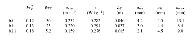
Dimensional values for DNS, including surface tension (b.i–b.iii), where
 $a_{\textit{res}}$
is the smallest bubble resolved by the grid. The Hinze scale
 $a_H$
is calculated using (3.11).

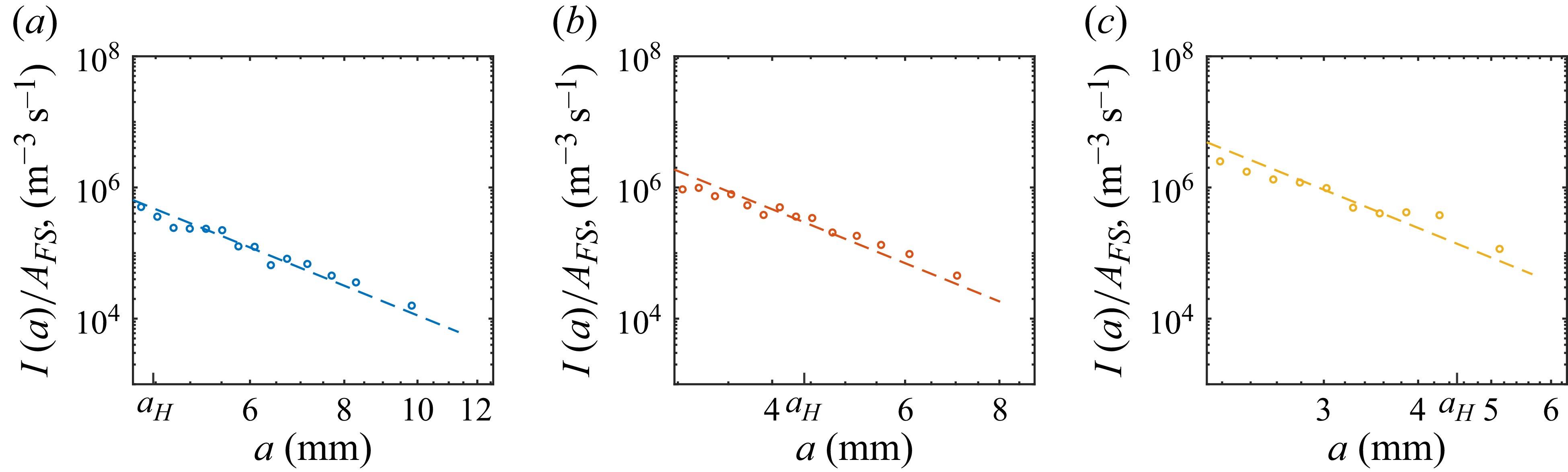
Entrainment size distribution (per unit free surface area) for (a)
 ${\textit{We}}_T=36$
, (b)
 ${\textit{We}}_T=25$
, and (c)
 ${\textit{We}}_T=5.2$
. In each plot, the dashed line shows the fit to (3.9) with the corresponding value of
 $C_I$
, and the Hinze scale
 $a_H$
given by (3.11) is indicated.

It is known that the influence of surface tension on bubble fragmentation causes a change in the entire bubble populations around the Hinze scale (Deane & Stokes Reference Deane and Stokes2002), defined as the bubble radius
 \begin{equation} a_H = 0.83 (\sigma /\rho _w)^{3/5} \varepsilon ^{-2/5}, \end{equation}
below which turbulent fragmentation is prevented by surface tension (Hinze Reference Hinze1955; Martínez-Bazán et al. Reference Martínez-Bazán, Montañés and Lasheras1999). For these simulations,
 $a_H\approx 4.4\ \mathrm{mm}$
. Figure 8 shows the obtained entrainment size distributions, and we highlight that for the large bubbles that we study (
 $a\gt a_c=1.3\ \mathrm{mm}$
), there is no departure from
 $I(a)\propto a^{-14/3}$
given by (3.9), including around
 $a_H$
. It is not surprising that the entrainment size distributions in figure 8 are unaffected by
 $a_H$
. This is because the Hinze scale comes from the relationship between surface tension and turbulence, where the entrainment of large bubbles is driven by the relationship between gravity and turbulence.
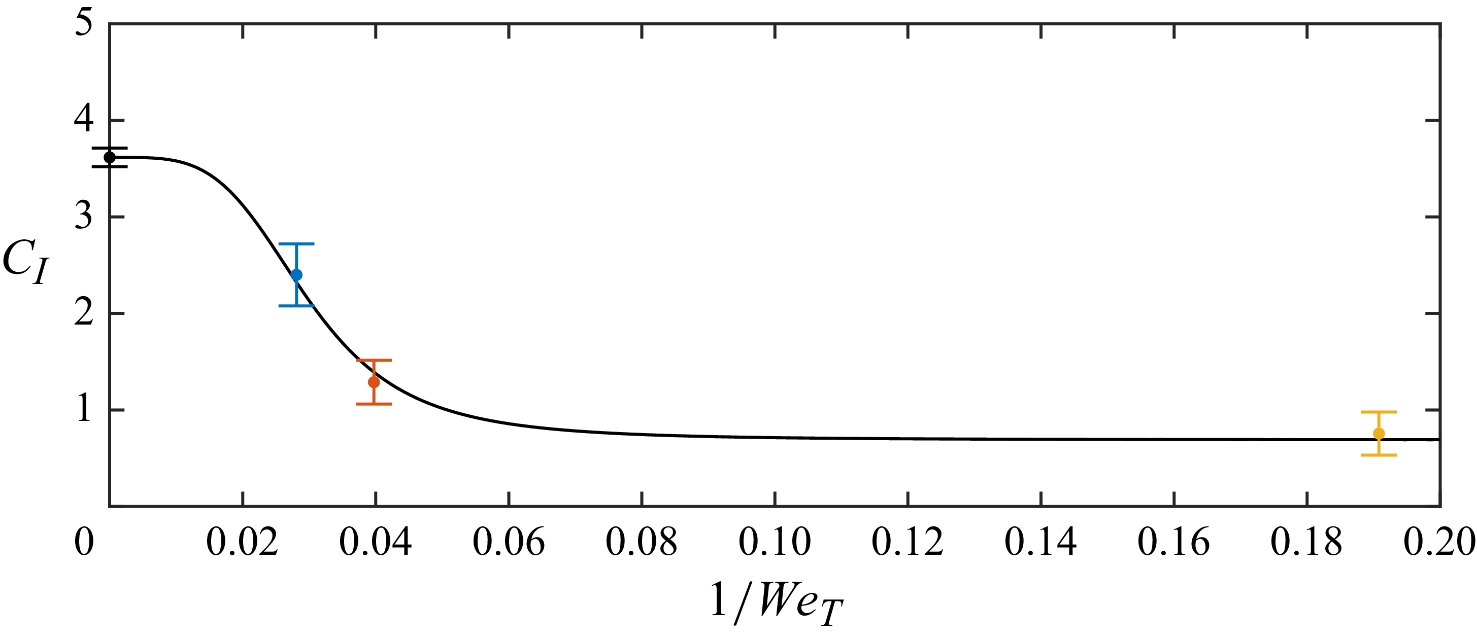
Value of
 $C_I$
obtained through regression as a function of
 ${\textit{We}}_T$
, with error bars indicating the 95
 $\%$
confidence intervals. The solid line shows the empirical fit, (3.12).

With the exception of the case with the strongest surface surface tension (b.iii) where surface tension suppresses
 $L_T$
, we also see that
 $a_{{max}} \approx 0.3 L_T$
, consistent with § 3.3. Rather than changes in the shape of
 $I(a)$
, we find that the effect of surface tension on large-bubble entrainment is to decrease the magnitude of
 $I(a)$
through
 $C_I$
. Consistent with
 $C_I({\textit{We}}_T\to \infty )=3.62$
from § 3.3, we use
 $C_I$
from these simulations to obtain the empirical fit
 \begin{equation} C_I(\textit{We}_T) = \frac {3.62-A}{1+ \left (\textit{We}_{T,{cr}}/\textit{We}_T\right )^{4}} + A {,} \end{equation}
where
 ${\textit{We}}_{T,{cr}}=34$
and
 $A=0.69$
, as shown in figure 9. While extending the model in § 2.2 to include surface tension effects could provide a mechanistic explanation for (3.12), a challenge is that
 $p\sim (\rho _w g + \sigma \kappa ^2) \eta$
would make the relationship between
 $\eta$
and
 $\kappa$
in (2.7) non-monotonic. Our results show that any effects of surface tension on the entrainment of large bubbles become negligible for
 ${\textit{We}}_T \gt \textit{We}_{T,{cr}}$
, which is reflected in the denominator of (3.12).
4. Entrainment by FST in general air-entraining flows
Our interest is the mechanism of bubble entrainment driven by strong FST. And for this purpose, we have studied a flow where the only mechanism present is FST. For general air-entraining flows, other entrainment mechanisms may also be present. However, in many of these flows, strong FST is clearly present (Brocchini & Peregrine Reference Brocchini and Peregrine2001). If the FST entrainment mechanism that we describe in this paper is the significant contribution to the total entrainment of a flow, then one would expect to see the FST scaling that we find manifest in the entrainment size distribution of the flow.
Entrainment size distribution for different turbulent Froude numbers
 ${\textit{Fr}}_T$
as measured by Gaylo et al. (Reference Gaylo, Hendrickson and Yue2024) in shear flow simulations. The dashed line shows our model (3.9) with
 $C_I=3.62$
(
 $R^2=0.891$
).

As an illustration of a more general air-entraining flow, we consider the canonical free-surface shear, where a velocity shear beneath an initially flat free surface generates waves and turbulence at the surface (Dimas & Triantafyllou Reference Dimas and Triantafyllou1994; Shen et al. Reference Shen, Zhang, Yue and Triantafyllou1999). This flow has been used as a model to study ship wakes. Despite the presence of the (directional) shear, at sufficiently large Froude number (consistent with strong FST), the near-surface turbulence is shown to be nearly isotropic (Yu et al. Reference Yu, Hendrickson, Campbell and Yue2019). From DNS of this canonical flow at a range of different
 ${\textit{Fr}}^2=U^2/L g$
(where
 $U$
and
 $L$
describe the speed and length of the shear profile), Gaylo et al. (Reference Gaylo, Hendrickson and Yue2024) use bubble tracking to obtain
 ${O}(10^4)$
entrainment events and the size distribution
 $I(a)$
. They also report
 ${\textit{Fr}}^2_T$
(which scales linearly with the shear flow
 ${\textit{Fr}}^2$
), allowing us to directly compare those results to our model. Even without adjusting
 $C_I=3.62$
, figure 10 shows that our model (3.9) for FST entrainment does a good job of predicting their measured
 $I(a)$
(in
 $\log$
-
 $\log$
space,
 $R^2=0.891$
) (cf. Gaylo et al. Reference Gaylo, Hendrickson and Yue2024, figure 4). While the existence of other entrainment mechanisms may cause the fit to be not quite as perfect as for our FST simulations (with
 $R^2=0.990$
), the still strong agreement suggests that the FST entrainment mechanism is the dominant entrainment mechanism for this free-surface shear flow.
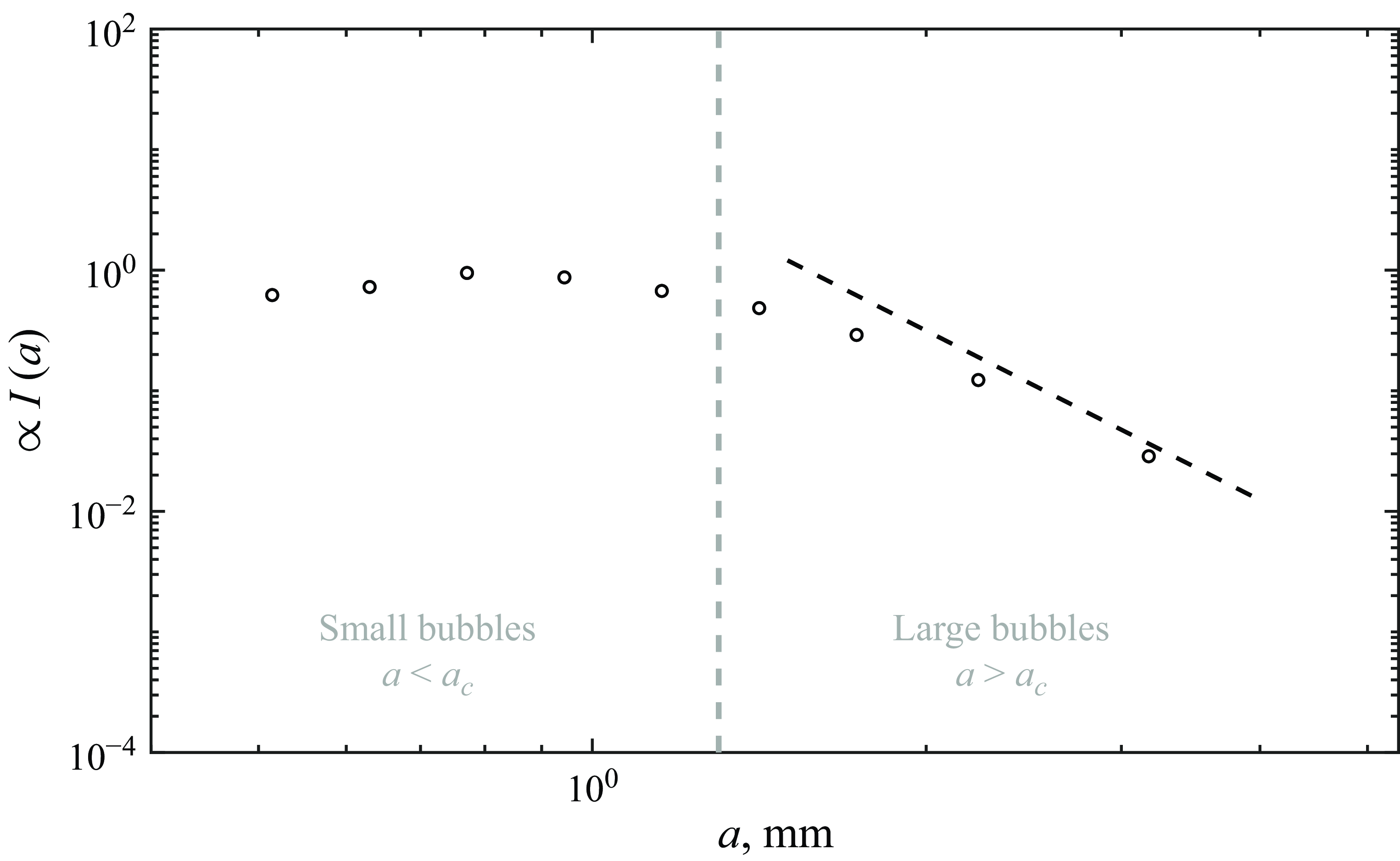
Entrainment size distribution calculated from the results of Wei et al. (Reference Wei, Xu, Deng, Tian and Zhang2019) for open channel flow experiments. The scaling of the
 $y$
-axis is arbitrary. The dashed line shows
 $I(a)\propto a^{-14/3}$
from (3.9).

As a second illustration, we consider open channel flow, a model of the flow in rivers and spillways. From experiments, Wei et al. (Reference Wei, Xu, Deng, Tian and Zhang2019) report the size of bubble produced by
 $108$
entrainment events. From their results, we can calculate the corresponding entrainment size distribution (figure 11). Because some entrainment events would have been obscured from view, and
 $A_{\textit{FS}}$
was not reported, the magnitude of
 $I(a)/A_{\textit{FS}}$
is unclear; however, we can still report the shape of
 $I(a)$
across radii. While there are only
 $108$
entrainment events, and many produce small bubbles (
 $a\lesssim a_c$
), we find that in the limit
 $a\gg a_c$
, the results appear to be converging to
 $I(a)\propto a^{-14/3}$
from (3.9).
5. Conclusion
Air-entraining flow is relevant to a wide variety of natural and engineering applications. Due to the size-dependent properties of bubbles, e.g. the ratio of surface area to volume for gas transfer or the resonant frequency for acoustics, predicting the size distribution of the resulting bubble population is important to many of these applications. For a general description of the size distribution of bubble populations, individual models for each physical mechanism are necessary. For entrainment of bubbles, different mechanisms could be involved for different physical flows. However, a common feature of many air-entraining flows is the presence of strong turbulence beneath the free surface. In this work, we specifically address entrainment by this strong free-surface turbulence (FST), and characterise the size distribution of bubbles larger than the capillary scale
 $a_c\approx 1.3\ \mathrm{mm}$
.
We find that for strong FST, the near-surface turbulence is nearly isotropic. From this observation, dimensional analysis in § 2.1 shows that large-bubble FST entrainment is governed by a single scaling parameter
 $\alpha$
and a scaling constant
 $C_I$
. Using DNS of forced turbulence under a free surface, which isolates the FST entrainment mechanism, we obtain
 $\alpha =6$
and
 $C_I\approx 3.62$
. This gives (3.9) to describe how large-bubble entrainment scales with gravity, the strength of turbulence, and bubble radius. We show that nearly isotropic near-surface turbulence (defining strong FST) is obtained for turbulent
 ${\textit{Fr}}_T^{\kern1pt 2}\geqslant 0.1$
. We find that (3.9), based on near-surface isotropic turbulence, strongly agrees with the measured distributions (
 $R^2=0.990$
), even when including
 ${\textit{Fr}}_T^{\kern1pt 2}\lesssim 0.1$
. For this isotropic turbulence, we describe the mechanism for FST entrainment, which is consistent with observations of entrainment events, and obtain the same
 $g^{-3}$
(i.e.
 ${\textit{Fr}}_T^6$
) and
 $a^{-14/3}$
scaling of the entrainment size distribution. Introducing weak surface tension effects, we find that surface tension decreases
 $C_I$
, but
 $I(a)\propto a^{-14/3}$
from (3.9) is true for all
 $a\gt a_c$
. Strong surface tension effects (or equivalently small bubbles
 $a\lt a_c$
) are outside the limits of the DNS that we perform. While our analysis of the experimental results of Wei et al. (Reference Wei, Xu, Deng, Tian and Zhang2019) gives some indication (see figure 11), many more observations will be necessary to obtain definitive entrainment statistics in this regime. We note that a description of
 $I(a)$
across all bubble sizes will be necessary to calculate the total flux of air.
We study a flow chosen to isolate entrainment by FST, but find that our results apply to more general, complex flows where other entrainment mechanisms could be present. For both a shear flow and an open channel flow, the agreement between
 $I(a)$
observed and our model both serves as further validation of our model and suggests that FST entrainment is the dominant entrainment mechanism in these flows. We note that there are a myriad of air-entraining flows, and some involve different (dominant) entraining mechanisms, notably cavity entrapment in breaking waves (Gao et al. Reference Gao, Deane and Shen2021b
) or plunging jets (Kiger & Duncan Reference Kiger and Duncan2012). While we do not expect one model to be able to explain the features of all conceivable air-entraining flows, if entrainment by FST mechanism is a significant contributor to the total entrainment, then one expects to see its features reflected in
 $I(a)$
. Noting the common presence of near-surface turbulence (Brocchini & Peregrine Reference Brocchini and Peregrine2001), this suggests that our model for FST entrainment will contribute to the understanding of broad classes of air-entraining free-surface flows.
Acknowledgements
The authors thank Dr K. Hendrickson for collaboration on the DNS solver.
Funding
This work was funded by the US Office of Naval Research grant N00014-24-1-2076 under the oversight of Dr W.-M. Lin and Dr Y.L. Young. The computational resources were funded through the Department of Defense High Performance Computing Modernization Program.
Declaration of interests
The authors report no conflict of interest.