



1. Introduction
Taylor–Couette (TC) flow, the motion of fluid between two coaxial cylinders with one or both rotating, has served for over a century as a canonical system for investigating hydrodynamic stability and transition to turbulence (Couette Reference Couette1890; Taylor Reference Taylor1923). For Newtonian fluids with a fixed outer cylinder, the flow is governed by the inner Reynolds number
 $\textit{Re}=\rho \omega _{i}r_{i}d/\mu$
. At low
 $\textit{Re}$
, the flow is purely azimuthal circular Couette flow (CCF) (Couette Reference Couette1890). Beyond a critical value
 $\textit{Re}_{c,1}$
, centrifugal instability gives rise to steady, axisymmetric toroidal Taylor vortex flow (TVF) (Taylor Reference Taylor1923), which in turn becomes unstable to time-dependent wavy vortex flow (WVF) at a secondary critical Reynolds number
 $\textit{Re}_{c,2}$
(Andereck et al. Reference Andereck, Liu and Swinney1986). This rich bifurcation cascade has motivated extensive studies on the influence of non-Newtonian rheology, particularly shear-thinning, a nonlinear decrease in viscosity with shear rate,
 $\mu \sim \dot \gamma ^{n-1}$
(
 $n\le 1$
), which is ubiquitous in polymer solutions, suspensions and biological fluids (Mueller et al. Reference Mueller, Llewellin and Mader2010; Larson & Desai Reference Larson and Desai2015; Majji et al. Reference Majji, Banerjee and Morris2018). In TC flow, the spatial variation of viscosity necessitates a reference scale; while various choices exist (Masuda et al. Reference Masuda, Horie, Hubacz, Ohta and Ohmura2017), the nominal shear rate
 $\dot \gamma _{nom}=\omega _{i}r_{i}/d$
is most common (Cagney & Balabani Reference Cagney and Balabani2019; Cagney et al. Reference Cagney, Lacassagne and Balabani2020; Elçiçek & Güzel Reference Elçiçek and Güzel2020). For the primary instability (CCF
 $\rightarrow$
TVF) in narrow gaps (
 $\eta =r_i/r_o\ge 0.8$
), linear stability analyses and numerical studies consistently predict that enhanced shear-thinning (decreasing
 $n$
) reduces
 $\textit{Re}_{c,1}$
, provided the Reynolds number is defined using the zero-shear-rate viscosity (Lockett et al. Reference Lockett, Richardson and Worraker1992; Coronado-Matutti et al. Reference Coronado-Matutti, Souza Mendes and Carvalho2004; Ashrafi Reference Ashrafi2011; Alibenyahia et al. Reference Alibenyahia, Lemaitre, Nouar and Ait-Messaoudene2012). This destabilisation is attributed to reduce near-wall viscosity, which amplifies local centrifugal effects, and is accompanied by a profound modification of the TVF structure, including vorticity concentration at outflow boundaries and a strong asymmetry between inward and outward radial jets (Topayev et al. Reference Topayev, Nouar, Bernardin, Neveu and Bahrani2019; Cagney & Balabani Reference Cagney and Balabani2019).
In contrast, the influence of shear-thinning on the secondary instability (TVF
 $\rightarrow$
WVF) remains poorly understood and experimentally contentious. In a narrow-gap configuration (
 $\eta =0.83$
) with aspect ratio
 $\varGamma =12.97$
, Cagney & Balabani (Reference Cagney and Balabani2019) reported a non-monotonic dependence of
 $\textit{Re}_{c,2}$
on
 $n$
(
 $\textit{Re}_{c,2} = 664$
for
 $n = 0.52$
,
 $\textit{Re}_{c,2} \gt 874$
for
 $n = 0.62$
and
 $\textit{Re}_{c,2} = 826$
for
 $n = 0.68$
), with the WVF transition vanishing for intermediate
 $n$
, alongside slow axial vortex drift and spatially varying wave amplitudes. In another finite-length experiment with a similar radius ratio (
 $\eta =0.8$
) but a lower aspect ratio (
 $\varGamma =6.0$
), Kawaguchi et al. (Reference Kawaguchi, Tano and Saito2022) studied two shear-thinning fluids (
 $n=0.7$
and
 $0.52$
) and found that
 $\textit{Re}_{c,2}$
dropped significantly from 1330 (Newtonian) to 608.7 for
 $n=0.7$
and 93.1 for
 $n=0.52$
, exhibiting a monotonic dependence on
 $n$
, yet they observed pronounced axial elongation of end vortices and drift of vortex centres, features absent in their Newtonian counterpart. Meanwhile, Elçiçek & Güzel (Reference Elçiçek and Güzel2020) observed a direct transition from TVF to modulated wavy flow in xanthan gum solutions, bypassing the classic WVF regime entirely. These contradictory experimental outcomes strongly implicate endwall-induced finite-length effects, which constrain the axial wavelength and suppress the amplitude of the azimuthal waves. These contradictory experimental outcomes strongly implicate endwall-induced finite-length effects, which constrain the axial wavelength and suppress the amplitude of the azimuthal waves. Previous theoretical and numerical works by Cole (Reference Cole1976), Jones (Reference Jones1985) and Topayev et al. (Reference Topayev, Nouar and Dusek2022) have demonstrated that such confinement effects can significantly delay or alter the secondary bifurcation, obscuring the intrinsic rheological stability of the shear-thinning fluid.
Therefore, two fundamental questions arise. (a) Does shear-thinning intrinsically stabilise or destabilise the secondary instability? (b) What physical mechanism underlies this effect? To isolate the fundamental role of shear-thinning on the two successive bifurcations in a narrow gap, we perform high-resolution direct numerical simulations (DNS) with axially periodic boundary conditions, thereby removing the influence of endwalls that are always present in experiments, and match the geometry of Cagney & Balabani (Reference Cagney and Balabani2019) (
 $\eta =0.83$
). This configuration enables a direct assessment of the intrinsic stability characteristics free from extrinsic wavelength constraints. The present work addresses two specific questions: whether shear-thinning intrinsically stabilises or destabilises the secondary instability, and what the underlying physical mechanism is. The remainder of this paper is organised as follows. We first briefly describe the numerical method and setting in § 2. Section 3 presents and analyses the results for radial viscosity variation and reveals the mechanism for the opposing effects of shear-thinning on primary and secondary instabilities. Finally, the work is concluded in § 4.
(a) Sketch of the TC system. (b–d) Verification of the Carreau model implementation at Re = 40, corresponding to the CCF regime. Symbols denote the viscosity computed from the DNS at various shear rates for
 $n=0.52$
,
 $0.62$
, and
 $0.68$
; solid lines represent the theoretical Carreau model (2.5) with parameters from table 1.

Figure 1. Long description
Panel A: A diagram of the Taylor-Couette (TC) system. The diagram shows a cylindrical setup with an inner cylinder of radius ri, an outer cylinder of radius ro, and a length L. The inner cylinder rotates with an angular velocity ωi, and the distance between the cylinders is denoted as d. Panel B: A line graph showing the verification of the Carreau model implementation at Re = 40, corresponding to the CCF regime. The x-axis is labeled λcβ and the y-axis is labeled μ(β)/μ0. The graph includes orange circles representing the viscosity computed from the DNS at various shear rates for n = 0.52, and a solid line representing the theoretical Carreau model. Panel C: A line graph showing the verification of the Carreau model implementation for n = 0.62. The x-axis is labeled λcβ and the y-axis is labeled μ(β)/μ0. The graph includes blue circles representing the viscosity computed from the DNS at various shear rates, and a solid line representing the theoretical Carreau model. Panel D: A line graph showing the verification of the Carreau model implementation for n = 0.68. The x-axis is labeled λcβ and the y-axis is labeled μ(β)/μ0. The graph includes red circles representing the viscosity computed from the DNS at various shear rates, and a solid line representing the theoretical Carreau model.
2. Numerical method and setting
The TC system consists of two concentric cylinders, as shown in figure 1(a). In the present study, the outer cylinder is at rest, the inner cylinder is rotating at angular velocity
 $\omega _i$
and thus driving the flow. Both inner and outer walls are smooth and set as the no-slip boundary condition. To eliminate endwall effects inherent in experimental setups and isolate the intrinsic stability characteristics of the flow, axially periodic boundary conditions are imposed in the axial direction. The radius ratio is fixed at
 $\eta = r_{i}/r_{o} = 0.83$
, matching the experimental configuration of Cagney & Balabani (Reference Cagney and Balabani2019) to facilitate direct comparison. In addition, this narrow-gap configuration minimises curvature effects and allows the radial viscosity variation to be isolated from curvature-induced complexities; the base flow velocity profile is approximately linear, which facilitates interpretation. For wider gaps (
 $\eta \le 0.7$
), however, curvature effects become significant, and shear-thinning may interact with them to qualitatively modify the instability mechanisms. The axial periodicity length is set to
 $L = 2\pi d$
, corresponding to an aspect ratio
 $\varGamma = L/d = 2\pi$
. This choice accommodates exactly three pairs of Taylor vortices, based on the experimentally observed wavelength of approximately
 $2.16d$
for the Newtonian case (Cagney & Balabani Reference Cagney and Balabani2019).
The working fluid is assumed to be incompressible and purely shear-thinning, with no viscoelastic effects. The flow is governed by the continuity and Navier–Stokes equations:
 \begin{equation} \boldsymbol{\nabla }\boldsymbol{\cdot }\boldsymbol{u}=0, \end{equation}
 \begin{equation} \frac {\partial \boldsymbol{u}}{\partial t}+\boldsymbol{\nabla }\boldsymbol{\cdot }(\boldsymbol{uu})=-\frac {1}{\rho }\boldsymbol{\nabla }p+\frac {1}{\rho }\boldsymbol{\nabla }\boldsymbol{\cdot }\boldsymbol{\tau }, \end{equation}
where
 \begin{equation} \boldsymbol{\tau } = \mu (\dot \gamma )(\boldsymbol{\nabla }\boldsymbol{u} + (\boldsymbol{\nabla }\boldsymbol{u})^T), \end{equation}
where
 $\boldsymbol{u}$
, t and p are the velocity, time and pressure of the flow;
 $\rho$
and
 $\mu (\dot \gamma )$
are the density and the dynamic viscosity of the fluid, respectively. It should be noted that
 $\boldsymbol{\nabla }\boldsymbol{\cdot }[\mu (\dot \gamma )\boldsymbol{\nabla }\boldsymbol{u}]$
cannot be simplified to
 $\mu (\dot \gamma )\boldsymbol{\nabla} ^2\boldsymbol{u}$
unless the viscosity is spatially constant. In the present study, the simulations are performed using the standard finite-volume solver in OpenFOAM, where the viscous term is discretised directly in the conservative stress-divergence form based on (2.3), and the viscosity is updated at each cell face according to the local velocity gradients using the Carreau model. Thus, the spatial viscosity variations are rigorously accounted for. The equations are non-dimensionalised using the gap width
 $d$
as the length scale, the inner cylinder tangential velocity
 $u_i = r_i\omega _i$
as the velocity scale, the large-eddy turnover time
 $t^{\ast }$
=
 $d/u_i$
, and the inertial pressure scale
 $\rho u_i^2$
. We also define the non-dimensional radius
 $r^{\ast }$
to be
 $r^{\ast }$
= (
 $r- r_{i}$
)/d.
In TC flow, the Reynolds number is defined as
 \begin{equation} Re=\frac {\rho \omega _{i}r_{i}d}{\mu _{ref}}, \end{equation}
where the reference viscosity
 $\mu _{ref}$
is evaluated at the nominal shear rate
 $\dot \gamma _{nom} = \omega _i r_i / d$
, following the convention established for shear-thinning TC flow (Cagney & Balabani Reference Cagney and Balabani2019). The shear-rate-dependent viscosity is described by the Carreau model:
 \begin{equation} \mu (\dot \gamma )=\mu _{\infty }+(\mu _{0}-\mu _{\infty })[1+(\lambda _{c}\dot \gamma )^2]^{(n-1)/2}, \end{equation}
where
 $\mu _{0}$
and
 $\mu _{\infty }$
are the zero- and infinite-shear-rate viscosities,
 $\lambda _{c}$
is the characteristic relaxation time and
 $n$
is the shear-thinning index (
 $n=1$
for a Newtonian fluid).
Equations (2.1) and (2.2) are solved using the open-source finite-volume platform OpenFOAM. A second-order-accurate, collocated grid arrangement is employed. Temporal discretisation uses the second-order backward scheme, while the convective terms are discretised with a second-order total variation diminishing (Van Leer) scheme. The computational domain is discretised using a structured mesh with
 $N_r = 64$
,
 $N_\theta = 256$
and
 $N_z = 128$
cells in the radial, azimuthal and axial directions, respectively. The mesh is refined in the near-wall regions to adequately resolve the steep velocity gradients and the thin boundary layers characteristic of shear-thinning TC flow. The minimum radial grid spacing near the walls is approximately
 $0.008d$
, while the maximum spacing in the gap centre is
 $0.03d$
. The azimuthal and axial directions employ uniform meshes with spacings of approximately
 $0.13d$
and
 $0.05d$
, respectively. A fixed time step is chosen such that the Courant–Friedrichs–Lewy (CFL) number remains below 0.7 throughout all simulations. As a global measure of numerical convergence, we monitor the torque conservation for every Reynolds number. In all cases, the relative difference between the torque acting on the inner cylinder and that acting on the outer cylinder remains below 1 % after the flow reaches a statistically steady state. The simulations are advanced until the time-averaged torques on the inner and outer cylinders differ by less than 1 %, and statistics are collected over at least 100 large-eddy turnover times (
 $d/u_i$
) after this quasi-steady state is reached (Dong Reference Dong2007; Brauckmann & Eckhardt Reference Brauckmann and Eckhardt2013). Velocity and pressure fields computed in Cartesian coordinates are transformed to cylindrical coordinates for post-processing.
The solver has been validated for Newtonian TC flow in our previous work (Xu et al. Reference Xu, Su, Lan, Zhao, He, Sun and Wang2022, Reference Xu, Zhao, Sun, He and Wang2023) and further verified for shear-thinning fluids by comparing DNS-based effective viscosities with the Carreau model at low
 $\textit{Re}$
(Re = 40), where the flow is purely azimuthal. The agreement confirms correct implementation of the rheology (figure 1
b–d). To determine the critical Reynolds numbers
 $\textit{Re}_{c,1}$
and
 $\textit{Re}_{c,2}$
, the simulations are initiated from a low Reynolds number
 $\textit{Re}=40$
, where the flow remains in the CCF state. The Reynolds number was increased gradually in coarse steps to identify the approximate onset of the TVF state. Once the TVF state was established, the Reynolds number was reduced back into the stable CCF regime to obtain a robust initial condition. Subsequently,
 $\textit{Re}$
was increased again with a much finer increment of
 $\Delta Re = 1$
to accurately determine the critical Reynolds number for the primary instability
 $\textit{Re}_{c,1}$
. The same procedure was applied for the secondary transition from TVF to WVF. The onset of TVF is identified by steady axisymmetric vortex structures, while WVF is detected by the emergence of travelling azimuthal waves, as verified by the time series of the axial velocity at multiple monitor points. For each fluid, simulations are conducted up to
 $\textit{Re} \approx 1000$
, sufficient to capture both instabilities. Results at higher
 $\textit{Re}$
are provided in the supplementary material. Three shear-thinning indices (
 $n=0.52, 0.62, 0.68$
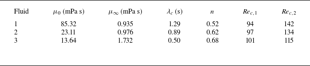
) are considered using parameters listed in table 1, taken from Cagney & Balabani (Reference Cagney and Balabani2019). The critical Reynolds numbers obtained from the present DNS for each fluid are also included in table 1.
Carreau model parameters for the three shear-thinning fluids investigated (reproduced from Cagney & Balabani (Reference Cagney and Balabani2019)) together with the critical Reynolds numbers
 $\textit{Re}_{c,1}$
and
 $\textit{Re}_{c,2}$
obtained from the present DNS. Here
 $\mu _0$
and
 $\mu _{\infty }$
are the zero- and infinite-shear-rate viscosities,
 $\lambda _c$
is the characteristic relaxation time and
 $n$
is the shear-thinning index.

Table 1. Long description
A table comparing parameters of three shear-thinning fluids. The table has three rows and six columns. Column headers are Fluid, μ0 (mPa s), μ∞ (mPa s), λc (s), n, Rec,1, and Rec,2. Row 1: Fluid, 1; μ0 (mPa s), 85.32; μ∞ (mPa s), 0.935; λc (s), 1.29; n, 0.52; Rec,1, 94; Rec,2, 142. Row 2: Fluid, 2; μ0 (mPa s), 23.11; μ∞ (mPa s), 0.976; λc (s), 0.89; n, 0.62; Rec,1, 97; Rec,2, 134. Row 3: Fluid, 3; μ0 (mPa s), 13.64; μ∞ (mPa s), 1.732; λc (s), 0.50; n, 0.68; Rec,1, 101; Rec,2, 115.
3. Results and discussion
Figure 2(a) summarises the critical Reynolds numbers for the onset of TVF (
 $\textit{Re}_{c,1}$
) and WVF (
 $\textit{Re}_{c,2}$
) as functions of the shear-thinning index
 $n$
, obtained from the present DNS and compared with the experimental measurements of Cagney & Balabani (Reference Cagney and Balabani2019). The phase diagram in figure 2(a) delineates the stability boundaries separating the CCF, TVF and WVF regimes (Andereck et al. Reference Andereck, Liu and Swinney1986). Figure 2(b) displays representative contours of the azimuthal vorticity in the meridional (
 $r$
–
 $z$
) plane for the TVF and WVF regimes, illustrating the structural changes in the flow associated with each instability.
(a) Critical Reynolds numbers for the onset of TVF (
 $\textit{Re}_{c,1}$
) and WVF (
 $\textit{Re}_{c,2}$
) as functions of the shear-thinning index
 $n$
. The DNS results are shown as open symbols connected by lines, while the open symbols denote the experimental data of Cagney & Balabani (Reference Cagney and Balabani2019). The regimes CCF, TVF and WVF are denoted by text labels in the diagram. (b) Instantaneous contours of the azimuthal vorticity (normalised by the rotating angular velocity of inner cylinder) in the meridional (
 $r{-}z$
) plane at two azimuthal positions (
 $\theta =0$
and
 $\theta =\pi$
) for TVF (
 $\textit{Re}_{c,1}=94$
) and WVF (
 $\textit{Re}_{c,2}=142$
) at
 $n=0.52$
. The steady axisymmetric TVF structure and the symmetry breaking in WVF are clearly visible. Three triangular markers at
 $z = L/4$
,
 $L/2$
and
 $3L/4$
are superimposed on the WVF contour at
 $\theta =0$
, indicating the locations of the three monitor points used in (c); all three probes are at the mid-gap
 $r^*=0.5$
. (c) Time evolution of the axial velocity
 $u_z/u_i$
at the mid-gap (
 $r^*=0.5$
) for
 $n=0.52$
, recorded at three axial monitor points (
 $z=L/4, L/2, 3L/4$
). Dashed lines denote the steady state at the primary instability threshold (
 $\textit{Re}_{c,1}=94$
), while solid lines illustrate the quasi-periodic oscillations at the secondary instability threshold (
 $\textit{Re}_{c,2}=142$
). The overlapping traces confirm the existence of an axially coherent, global travelling wave in the WVF regime. (d) Circumferential profile of
 $u_z/u_i$
at the mid-gap (
 $r^*=0.5$
) for
 $n=0.52$
(the corresponding profiles for other
 $n$
values are provided in the Appendix C). The profile exhibits three complete wave periods, corresponding to a dominant azimuthal mode m = 3.

For the primary instability (CCF
 $\rightarrow$
TVF), the DNS results reveal a clear monotonic trend: as the fluid becomes more shear-thinning (decreasing
 $n$
), the critical Reynolds number
 $\textit{Re}_{c,1}$
decreases from
 $101$
at
 $n=0.68$
to
 $94$
at
 $n=0.52$
. This destabilising effect is consistent with the physical picture that enhanced shear-thinning reduces the effective viscosity in the high-shear region adjacent to the inner cylinder, thereby amplifying the local centrifugal forces that drive the Taylor instability (Alibenyahia et al. Reference Alibenyahia, Lemaitre, Nouar and Ait-Messaoudene2012; Khali et al. Reference Khali, Nebbali and Bouhadef2013; Cagney & Balabani Reference Cagney and Balabani2019). In contrast, for the secondary instability (TVF
 $\rightarrow$
WVF), shear-thinning stabilises the wavy mode:
 $\textit{Re}_{c,2}$
increase from
 $115$
at
 $n=0.68$
to
 $142$
at
 $n=0.52$
. This opposing effect implies that the radial viscosity variation, while promoting centrifugal destabilisation, simultaneously suppresses the oscillatory shear-layer instability associated with inflectional velocity profiles between adjacent vortices. The experimental data of Cagney & Balabani (Reference Cagney and Balabani2019), however, exhibit a distinctly different, non-monotonic behaviour for both instabilities. It should be noted that the experimental values of
 $\textit{Re}_{c,2}$
are consistently far larger than their DNS counterparts. These discrepancies are direct manifestations of endwall effects inherent in finite-length experimental setups (Ji et al. Reference Ji, Burin, Schartman and Goodman2006), which are absent in the present axially periodic DNS (Cole Reference Cole1976; Czarny et al. Reference Czarny, Serre, Bontoux and Lueptow2003). While no-slip endwalls impose axial wavelength constraints, the axially periodic boundary conditions used here also restrict the admissible axial wavelengths. The key distinction is that the rigid endwalls mechanically suppress the amplitude of the travelling azimuthal waves that characterise the WVF regime (Cole Reference Cole1976; Jones Reference Jones1985), thereby artificially elevating the apparent
 $\textit{Re}_{c,2}$
. Indeed, the significant spatial variability of wave amplitudes observed in the experiments of Cagney & Balabani (Reference Cagney and Balabani2019) for shear-thinning fluids is itself a signature of these endwall-induced constraints. In contrast, the periodic boundary condition allows the travelling wave to propagate continuously across the axial boundaries without endwall-induced damping.
The vorticity contours in figure 2(b) provide structural evidence for the two distinct flow states. In the TVF regime, the azimuthal vorticity appears as three regularly spaced, alternating-sign vortex pairs along the axial direction, consistent with the imposed axial periodicity of
 $\varGamma = 2\pi$
. The steady, axisymmetric nature of these Taylor vortices is confirmed by the constant-time signals at the three monitor points shown in figure 2(c). The spatial structure emerges spontaneously from the nonlinear evolution within the periodic domain rather than from any prescribed forcing. Even if the axial length
 $L$
accommodates an integer number of vortex pairs, the vortex boundaries do not necessarily coincide with the periodic boundaries. In the present simulations, the observed alignment is a natural consequence of the specific mode selected during the nonlinear evolution, rather than a prescribed condition or an artefact of the chosen axial length. Upon transition to WVF, this symmetry is broken: the vorticity contours become distorted and lose their axial regularity, indicative of the travelling azimuthal waves that characterise the wavy instability (Wereley & Lueptow Reference Wereley and Lueptow1998). Overall, shear-thinning has a destabilising effect on the primary instability but a significantly stronger stabilising effect on the secondary instability.
The rheological parameters in table 1 are extracted from the experimental fluids, where
 $\mu _0$
,
 $\mu _\infty$
,
 $\lambda _c$
and
 $n$
vary simultaneously. To isolate the individual influence of the shear-thinning index
 $n$
from the viscosity levels themselves, we performed a controlled set of simulations where
 $\mu _0$
,
 $\mu _\infty$
and
 $\lambda _c$
were fixed while
 $n$
was varied. The results confirm that the opposing trends are robust regardless of whether the other Carreau parameters are varied or fixed: a decreasing
 $n$
consistently lowers
 $\textit{Re}_{c,1}$
and elevates
 $\textit{Re}_{c,2}$
. The quantitative differences observed between the fixed-parameter simulations and the original experimental fluids, such as the variation in
 $\textit{Re}_{c,2}$
for
 $n=0.68$
, arise primarily from the substantial differences in the absolute viscosity levels. The parameters and numerical results of these controlled simulations are provided in Appendix A. We also validated our numerical framework against the linear stability benchmarks of Alibenyahia et al. (Reference Alibenyahia, Lemaitre, Nouar and Ait-Messaoudene2012) for power-law fluids. Although their results were obtained for a slightly different radius ratio and for a power-law rather than Carreau rheology, both sets exhibit the same physical trend:
 $\textit{Re}_{c,1}$
decreases monotonically with decreasing n when the Reynolds number is defined using the nominal shear-rate viscosity. This consistency confirms the reliability of our DNS methodology for capturing the primary instability. The parameters and numerical results of this validation are provided in Appendix B.
Furthermore, the use of axially periodic boundary conditions imposes a constraint on the admissible axial wavelengths. To evaluate the sensitivity of our results to the specific choice of the axial periodicity length, we performed additional simulations for the strongest shear-thinning fluid (
 $n=0.52$
) using two alternative periodic lengths (
 $L=6d$
and
 $L=6.6d$
). The resulting critical Reynolds numbers are as follows: for
 $L=6d$
,
 $\textit{Re}_{c,1}=94$
,
 $\textit{Re}_{c,2}=142$
; for
 $L=6.6d$
,
 $\textit{Re}_{c,1}=94$
,
 $\textit{Re}_{c,2}=141$
. These results demonstrate that the primary instability threshold (
 $\textit{Re}_{c,1}$
) is independent of the chosen periodic length, while the secondary instability threshold (
 $\textit{Re}_{c,2}$
) varies by only 1 Reynolds number unit. These findings confirm that the conclusions presented in this study are not artefacts of a specific axial wavelength selection, in line with the established understanding of wavelength constraints in periodic TC configurations (Cole Reference Cole1976; Jones Reference Jones1985; Topayev et al. Reference Topayev, Nouar and Dusek2022).
To further characterise the unsteady and three-dimensional features of the WVF regime, we present quantitative analyses in figures 2(c) and 2(d). Figure 2(c) shows the time evolution of the axial velocity
 $u_z$
at the mid-gap (
 $r^*=0.5$
) for
 $n=0.52$
, recorded at three distinct axial monitor points (
 $z=L/4, L/2, 3L/4$
). In the TVF regime,
 $u_z$
remains almost constant over time at all three positions, consistent with the steady, axisymmetric nature of Taylor vortices. As the flow transitions to WVF, the axial velocity at all three monitor points exhibits clear quasi-periodic oscillations. These quasi-periodic oscillations are captured at
 $\textit{Re}=\textit{Re}_{c,2}$
, the onset of the secondary instability. At this critical condition, the WVF perturbation has already emerged with a finite amplitude, as is typical for supercritical bifurcations in TC flow. Notably, the temporal signals from the three spatially separated axial points almost perfectly overlap, the maximum absolute deviation among the three signals is approximately 5 % of the signal amplitude, which is far smaller than the dynamic range of the oscillations and confirms that the three signals are indeed highly coherent. Although the three axial positions correspond to different local phases of the steady Taylor-vortex structure, the WVF perturbation itself is a global travelling wave that occupies the entire periodic domain (Wereley & Lueptow Reference Wereley and Lueptow1998). Because our simulations employ axially periodic boundary conditions, which eliminate the endwall-induced spatial damping that is inevitably present in experimental setups, the travelling wave is free to propagate without axial attenuation. Consequently, its axial envelope remains approximately uniform over the periodic length, yielding nearly identical amplitudes at all three monitoring points regardless of their different positions within the underlying vortex structure.
This interpretation is further supported by the observation that the dominant azimuthal mode m = 3 remains unchanged with n (figure 2(d) and Appendix C), confirming that the secondary instability is governed by a large-scale global mode rather than a locally confined fluctuation. Regarding the azimuthal structure, figure 2(d) presents the circumferential profiles of
 $u_z$
for the n = 0.52 case at the mid-gap (
 $r^*=0.5$
) (the corresponding profiles for n = 0.62 and 0.68 are provided in Appendix C). The profiles consistently exhibit three complete wave periods for all the investigated
 $n$
values, confirming a dominant azimuthal mode of
 $m=3$
and the three-dimensional travelling-wave character of the WVF regime (Jones Reference Jones1985; Andereck et al. Reference Andereck, Liu and Swinney1986). More importantly, the fact that
 $m=3$
remains constant across the different
 $n$
values provides critical physical insight into the stabilising mechanism. It indicates that shear-thinning, while significantly postponing the onset of WVF (increasing
 $\textit{Re}_{c,2}$
), does not alter the preferred azimuthal mode selection. This implies that the stabilisation of the secondary instability originates from the enhanced viscous damping in the bulk gap that suppresses the growth of the travelling waves, rather than from a change in the spatial wavelength or mode structure.
It is also worth clarifying that the apparent shrinking of the Taylor-vortex stability range with increasing shear-thinning reported by Topayev et al. (Reference Topayev, Nouar, Bernardin, Neveu and Bahrani2019) is not in conflict with our present findings. This discrepancy originates from the different reference viscosity used in the definition of the Reynolds number. Following the convention of experimental studies (Cagney & Balabani Reference Cagney and Balabani2019), we define the Reynolds number using the viscosity evaluated at the nominal shear rate. In contrast, Topayev et al. (Reference Topayev, Nouar, Bernardin, Neveu and Bahrani2019) employed the zero-shear-rate viscosity
 $\mu _0$
as the reference. When our critical Reynolds numbers are recalculated using
 $\mu _0$
as the reference scale, the resulting values reproduce the qualitative trend reported by Topayev et al. (Reference Topayev, Nouar, Bernardin, Neveu and Bahrani2019), namely a shrinking TVF stability interval with decreasing
 $n$
. This demonstrates that the apparent contradiction is solely a consequence of the choice of the viscosity scale, rather than a conflict in the underlying physical mechanisms.
To clarify the physical mechanism underlying the contrasting effects of shear-thinning on
 $\textit{Re}_{c,1}$
and
 $\textit{Re}_{c,2}$
, we examine the radial profiles of the time- and spatially-averaged dimensionless viscosity and its gradient at the respective critical Reynolds numbers. Figure 3 presents these profiles for all three values of n, evaluated at
 $\textit{Re} = \textit{Re}_{c,1}$
(a,b) and
 $\textit{Re} = \textit{Re}_{c,2}$
(c,d). The viscosity is normalised by the viscosity
 $\mu {_0}$
at the zero shear rate, and the radial coordinate is
 $r^{\ast }$
= (
 $r-r_{i}$
)/d, with
 $r^{\ast }$
= 0 and
 $r^{\ast }$
= 1 corresponding to the inner and outer cylinder walls, respectively.
Radial profiles of the time-, azimuthally- and axially-averaged dimensionless viscosity
 $\mu (\dot \gamma )/\mu _0$
(a,c) and its radial gradient
 $\text{d}\mu (\dot \gamma )/\text{d}r$
(b,d) for three shear-thinning fluids with
 $n = 0.52$
,
 $0.62$
and
 $0.68$
. Panels (a,b) correspond to the primary instability threshold (
 $\textit{Re} = \textit{Re}_{c,1}$
); panels (c,d) correspond to the secondary instability threshold (
 $\textit{Re} = \textit{Re}_{c,2}$
). The dashed lines in (a,c) represent the average values of dimensionless viscosity at different n, and the dashed lines in (b,d) represent the radial gradient where
 $\text{d}\mu (\dot \gamma )/\text{d}r = 0$
.

Figure 3. Long description
The image contains four line graphs. Panel A shows the radial profiles of the time-, azimuthally- and axially-averaged dimensionless viscosity for three shear-thinning fluids with different values of n at the primary instability threshold. The x-axis is labeled r* and the y-axis is labeled μ(γ)/μ0. Panel B shows the radial gradient of the dimensionless viscosity for the same fluids and threshold, with the x-axis labeled r* and the y-axis labeled dμ(γ)/dr. Panel C presents similar data to Panel A but at the secondary instability threshold. Panel D presents similar data to Panel B but at the secondary instability threshold. Each graph includes dashed lines representing average values or gradients.
At the primary instability threshold (
 $\textit{Re} = \textit{Re}_{c,1}$
, figure 3
a,b), the viscosity profiles exhibit a pronounced variation across the gap for all shear-thinning cases. The vertical axes in figure 3 represent the normalised viscosity
 $\mu /\mu _0$
. As
 $n$
decreases, this normalised near-wall viscosity is substantially reduced, reflecting the stronger local shear-thinning effect described by the Carreau model, although the absolute viscosity
 $\mu _0$
for smaller
 $n$
remains higher (see table 1). This reduction is accompanied by a sharpening of the viscosity gradient
 $\text{d} \mu / \text{d} r$
in the inner region (
 $r^{\ast } \le 0.3$
), which reaches a maximum at approximately
 $r^{\ast } \approx 0.25$
in the inner portion of the gap and then decays towards the gap centre. The gradient values at the wall (
 $r^*=0$
) and at approximately
 $r^* \approx 0.45$
are comparable, indicating a non-monotonic gradient distribution. The enhanced positive gradient near the rotating inner cylinder effectively lubricates the flow, diminishing the local viscous resistance and thereby facilitating the centrifugal instability that triggers the formation of Taylor vortices (Ashrafi Reference Ashrafi2011; Alibenyahia et al. Reference Alibenyahia, Lemaitre, Nouar and Ait-Messaoudene2012).The subsequent negative gradient, although weaker, may further influence the radial distribution of angular momentum transport. Nevertheless, the overall effect accounts for the monotonic decrease of
 $\textit{Re}_{c,1}$
with decreasing
 $n$
observed in figure 2(a).
At the secondary instability threshold (
 $\textit{Re} = \textit{Re}_{c,2}$
, figure 3
c,d), the overall viscosity levels are lower than at
 $\textit{Re}_{c,1}$
due to the higher rotation rates, yet the qualitative trends with
 $n$
persist. Notably, the viscosity gradient profiles at
 $\textit{Re}_{c,2}$
display a more pronounced peak near the inner wall and a steeper decay in the outer region compared to those at
 $\textit{Re}_{c,1}$
. This intensified near-wall viscosity gradient has a dual effect. While it continues to promote centrifugal destabilisation, it also acts to confine the high-shear region to a thin boundary layer adjacent to the inner cylinder, leaving the bulk of the gap with a relatively elevated and more uniform viscosity. The wavy vortex instability, by contrast, is primarily associated with the destabilisation of the azimuthal velocity shear layers,
 $\partial u_\theta / \partial z$
, generated by the axial modulation of the Taylor vortex structure (Martinand et al. Reference Martinand, Serre and Lueptow2014; Dessup et al. Reference Dessup, Tuckerman, Wesfreid, Barkley and Willis2018). Shear-thinning stabilises the WVF by increasing the viscous damping of these shear layers, while the accompanying weakening of the radial jets further reduces the nonlinear coupling between adjacent vortices. Consequently,
 $\textit{Re}_{c,2}$
increases as
 $n$
decreases, yielding the opposing trend evident in figure 2(a).
The viscosity gradient profiles also reveal a subtle difference between the three fluids. For the most strongly shear-thinning case (
 $n=0.52$
), the gradient at
 $\textit{Re}_{c,2}$
reaches its maximum closer to the inner wall and decays more abruptly than for
 $n=0.62$
and
 $0.68$
. This correlates with the particularly pronounced stabilisation of the wavy mode observed for
 $n=0.52$
in figure 2(a). The radial confinement of the low-viscosity region thus appears to be a key factor in the suppression of the secondary instability.
In summary, the radial viscosity variation induced by shear-thinning exerts a dual influence: it promotes the primary centrifugal instability by reducing the effective viscosity near the driving wall, while it stabilises the secondary wavy instability by increasing the viscous damping in the bulk of the gap and restricting the low-viscosity region to a thin boundary layer. This differential effect constitutes the fundamental origin of the opposing effects reported in the present study. In the following section, we further explore this mechanism by analysing the full two-dimensional flow fields for the
 $n=0.52$
case at both critical Reynolds numbers.
To gain deeper insight into the mechanisms underlying the opposing stability trends, we now examine the full two-dimensional flow fields in the meridional (
 $r{-}z$
) plane for the most strongly shear-thinning fluid (
 $n=0.52$
). Figure 4 presents contours of the instantaneous dimensionless shear rate
 $\lambda {_c}\dot \gamma$
, viscosity
 $\mu _0$
, and azimuthal velocity
 $u_\theta /u_i$
superposed velocity vectors (the radial and axial components) at the critical Reynolds numbers for the primary instability (figure 4
a,
 $\textit{Re}_{c,1} = 94$
) and the secondary instability (figure 4
b,
 $\textit{Re}_{c,2} = 142$
). The local shear rate
 $\dot {\gamma }$
is calculated from the second invariant of the strain-rate tensor,
 $\dot {\gamma } = \sqrt {2\boldsymbol{D}:\boldsymbol{D}}$
, where
 $\boldsymbol{D} = (\boldsymbol{\nabla }\boldsymbol{u} + (\boldsymbol{\nabla }\boldsymbol{u})^T)/2$
is the strain-rate tensor.
Contours of the instantaneous (left) shear rate
 $\lambda _c\dot \gamma$
, (middle) dimensionless viscosity
 $\mu /\mu _0$
and (right) azimuthal velocity
 $u_\theta /u_i$
superposed velocity vectors (the radial and axial components) in the meridional (
 $r$
–
 $z$
) plane for the most shear-thinning fluid (
 $n = 0.52$
): (a) at the primary instability threshold (
 $\textit{Re}_{c,1} = 94$
) and (b) at the secondary instability threshold (
 $\textit{Re}_{c,2} = 142$
).

At
 $\textit{Re}_{c,1}$
(figure 4
a), the flow exhibits the characteristic structure of steady, axisymmetric TVF. Three counter-rotating vortex pairs are clearly discernible, regularly spaced along the axial direction with a wavelength corresponding to the imposed periodicity
 $\varGamma = 2\pi$
. The shear-rate field reveals concentrated bands of high
 $\dot \gamma$
adjacent to the inner cylinder wall and along the radial outflow jets separating adjacent vortices, where fluid is ejected from the inner boundary towards the outer cylinder. Correspondingly, the viscosity contours display pronounced spatial variations: the viscosity is lowest in the high-shear near-wall region and along the outflow jets, while significantly higher values occupy the vortex cores and the region near the stationary outer cylinder, where the local shear rate is diminished (Topayev et al. Reference Topayev, Nouar, Bernardin, Neveu and Bahrani2019). This spatial heterogeneity in viscosity is a direct consequence of the shear-thinning rheology and underpins the radial variation analysed in figure 3. The azimuthal velocity field shows the expected monotonic decay from the inner to the outer cylinder, with weak undulations induced by the toroidal vortices. The velocity vectors reveal a mild asymmetry: the outflow jet accelerates slightly as it moves outwards and the inflow jet decelerates gently inwards.
At
 $\textit{Re}_{c,2}$
(figure 4
b), the flow has transitioned to WVF, and the structural symmetry evident at
 $\textit{Re}_{c,1}$
is broken. The vortex boundaries are no longer straight axial lines; instead, they exhibit undulations characteristic of the travelling azimuthal waves that define the WVF regime (Andereck et al. Reference Andereck, Liu and Swinney1986; Wereley & Lueptow Reference Wereley and Lueptow1998). The shear-rate contours become distorted, with the outflow boundaries becoming inclined and tilted relative to the axial direction. The low-viscosity regions exhibit a similar tilted orientation to the outflow boundaries, and their shapes are similar across the flow field. Importantly, the azimuthal velocity field reveals a weakening of the inward jets relative to the outward jets, a feature that has been identified as a hallmark of shear-thinning TC flow (Escudier et al. Reference Escudier, Gouldson and Jones1995; Cagney & Balabani Reference Cagney and Balabani2019; Topayev et al. Reference Topayev, Nouar, Bernardin, Neveu and Bahrani2019). The velocity vectors in figure 4(b) show a much stronger asymmetry: the outflow jet accelerates rapidly as it moves outwards, while the inflow jet decelerates sharply when approaching the inner wall. This progression is consistent with the steeper viscosity gradient at the higher Reynolds number (figure 3
d): the low-viscosity zone adjacent to the inner wall facilitates outward acceleration, but the same zone fails to sustain the inward return flow, thereby weakening the inter-vortex coupling required for wavy instability. The reduced strength of the inward jets diminishes the axial modulation of the Taylor vortex structure, thereby weakening the azimuthal velocity shear layers,
 $\partial u_\theta / \partial z$
, which are the primary drivers of the wavy instability (Martinand et al. Reference Martinand, Serre and Lueptow2014; Dessup et al. Reference Dessup, Tuckerman, Wesfreid, Barkley and Willis2018). In other words, the inward jets are essential for sustaining the strong axial gradients of the azimuthal velocity that characterise the WVF regime (Jones Reference Jones1985). The diminished nonlinear coupling between adjacent vortices, combined with the elevated bulk viscosity noted in figure 3(c), thus provides a consistent explanation for the delayed onset of WVF with enhanced shear-thinning.
The contrasting flow structures at
 $\textit{Re}_{c,1}$
and
 $\textit{Re}_{c,2}$
thus corroborate the differential effect of shear-thinning on the two instabilities. At the primary threshold, the near-wall viscosity reduction dominates, promoting the centrifugal overturning that generates Taylor vortices. At the secondary threshold, however, the stabilising influences, elevated viscosity in the vortex cores, weakened inward jets and confinement of the low-viscosity region to a thin boundary layer, collectively outweigh any residual destabilising effects, leading to the observed increase in
 $\textit{Re}_{c,2}$
with decreasing
 $n$
.
4. Conclusions
DNS with axially periodic boundary conditions reveal that shear-thinning exerts opposing effects on successive instabilities in narrow-gap TC flow: enhanced shear-thinning (decreasing
 $n$
) destabilises the primary instability (
 $\textit{Re}_{c,1}$
decreases) but strongly stabilises the secondary instability (
 $\textit{Re}_{c,2}$
increases). This behaviour originates from a competition between two opposing consequences of radial viscosity variation: the reduced viscosity near the inner wall promotes centrifugal instability (destabilising), while the elevated viscosity in the bulk gap damps inter-vortex oscillations (stabilising). Comparison with experiments has demonstrated that previously reported non-monotonic trends arise from endwall-induced extrinsic constraints, such as wavelength confinement and amplitude suppression of the azimuthal waves, rather than intrinsic rheological effects. These findings establish the intrinsic bifurcation structure of shear-thinning TC flow in the narrow-gap configuration (
 $\eta =0.83$
) and clarify the distinct roles of rheology and conffnement in successive transitions.
Supplementary material
Supplementary material are available at https://doi.org/10.1017/jfm.2026.12226.
Funding
This study is financially supported by National Key R&D Program of China (grant number 2023YFE0106600) and National Natural Science Foundation of China (grant numbers 22421003 and 22508389).
Declaration of interests
The authors report no conflict of interest.
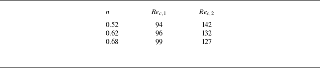
Appendix A. Details of the controlled simulations
The controlled simulations were performed with
 $\mu _0=85.32$
mPa s,
 $\mu _\infty =0.935$
mPa s and
 $\lambda _c=1.29$
s fixed at the values of the original
 $n=0.52$
fluid, while n was varied to 0.62 and 0.68. The resulting critical Reynolds numbers are summarised in table 2. These results confirm that the opposing trends are robust regardless of variations in the other Carreau parameters.
Critical Reynolds numbers obtained from controlled simulations, where only the shear-thinning index
 $n$
is varied, while
 $\mu _0, \mu _\infty$
and
 $\lambda _c$
are fixed at the values of the original
 $n=0.52$
fluid.

Table 2. Long description
A table with three rows and three columns. The columns are labeled n, Re_c,1, and Re_c,2. The row labels and values are as follows: Row 1: n, 0.52; Re_c,1, 94; Re_c,2, 142. Row 2: n, 0.62; Re_c,1, 96; Re_c,2, 132. Row 3: n, 0.68; Re_c,1, 99; Re_c,2, 127.
Appendix B. Validation against linear stability benchmarks
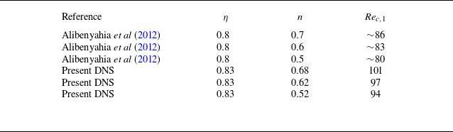
To demonstrate the numerical accuracy of our DNS methodology, we compare our results with the linear stability analysis of Alibenyahia et al. (Reference Alibenyahia, Lemaitre, Nouar and Ait-Messaoudene2012) for power-law fluids, as presented in table 3. The results of Alibenyahia et al. (Reference Alibenyahia, Lemaitre, Nouar and Ait-Messaoudene2012) (shown in their figure 8a) were obtained for a power-law fluid, whereas the present study employs the Carreau model. Despite these differences, both sets exhibit the same physical trend:
 $\textit{Re}_{c,1}$
decreases with decreasing n when defined using the nominal shear-rate viscosity, confirming the reliability of our DNS methodology.
Comparison of the primary instability threshold
 $\textit{Re}_{c,1}$
between the linear stability results of Alibenyahia et al. (Reference Alibenyahia, Lemaitre, Nouar and Ait-Messaoudene2012) using the power-law model and the present DNS using the Carreau model. Both sets exhibit the same physical trend, where decreasing
 $n$
leads to a lower
 $\textit{Re}_{c,1}$
, confirming the reliability of our numerical framework.

Table 3. Long description
A table with six rows and four columns comparing the primary instability threshold between the linear stability results of Alibenyahia et al. (2012) using the power-law model and the present DNS using the Carreau model. The columns are labeled Reference, η, n, and Re_c,1. Row 1: Reference Alibenyahia et al. (2012), η 0.8, n 0.7, Re_c,1 ~86. Row 2: Reference Alibenyahia et al. (2012), η 0.8, n 0.6, Re_c,1 ~83. Row 3: Reference Alibenyahia et al. (2012), η 0.8, n 0.5, Re_c,1 ~80. Row 4: Reference Present DNS, η 0.83, n 0.68, Re_c,1 101. Row 5: Reference Present DNS, η 0.83, n 0.62, Re_c,1 97. Row 6: Reference Present DNS, η 0.83, n 0.52, Re_c,1 94.
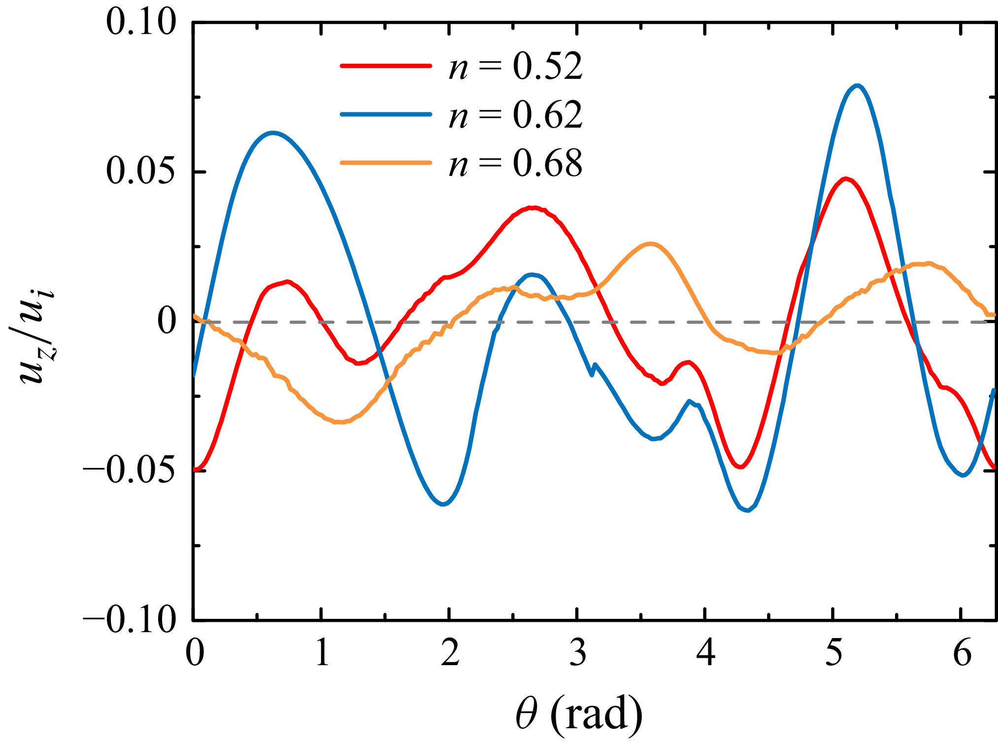
Circumferential profiles of
 $u_z/u_i$
at the mid-gap (
 $r^* = 0.5$
) for
 $n = 0.52$
,
 $0.62$
and
 $0.68$
, evaluated at their respective secondary instability thresholds (
 $\textit{Re} = \textit{Re}_{c,2}$
). All three profiles exhibit three complete wave periods, indicating a dominant azimuthal mode
 $m = 3$
that is independent of
 $n$
.

Appendix C. Circumferential profiles and azimuthal mode selection
As shown in figure 5, the circumferential profiles of the axial velocity
 $u_z/u_i$
at the mid-gap (
 $r^* = 0.5$
) for all three shear-thinning fluids exhibit three complete wave periods, corresponding to a dominant azimuthal mode
 $m = 3$
. The independence of
 $m$
from
 $n$
confirms that the stabilising effect originates from enhanced viscous damping in the bulk gap rather than from a change in the preferred azimuthal mode structure.

 n=0.52
 0.62
 0.68
 Rec,1
 Rec,2
 μ0
 μ∞
 λc
 n

 Rec,1
 Rec,2
 n
 r−z
 θ=0
 θ=π
 Rec,1=94
 Rec,2=142
 n=0.52
 z=L/4
 L/2
 3L/4
 θ=0
 r∗=0.5
 uz/ui
 r∗=0.5
 n=0.52
 z=L/4,L/2,3L/4
 Rec,1=94
 Rec,2=142
 uz/ui
 r∗=0.5
 n=0.52
 n

 μ(γ˙)/μ0
 dμ(γ˙)/dr
 n=0.52
 0.62
 0.68
 Re=Rec,1
 Re=Rec,2
 dμ(γ˙)/dr=0

 λcγ˙
 μ/μ0
 uθ/ui
 r
 z
 n=0.52
 Rec,1=94
 Rec,2=142
 n
 μ0,μ∞
 λc
 n=0.52
 Rec,1
 n
 Rec,1
 uz/ui
 r∗=0.5
 n=0.52
 0.62
 0.68
 Re=Rec,2
 m=3
 n



