2 Words to Numbers: Text Preprocessing Choices

Quantitative analysis requires that we transform our texts into numerical data. Accepting the wisdom that word order may be disposed of with minimal costs for inference (see Grimmer and Stewart Reference Grimmer and Stewart2013, for discussion)—and a ‘bag of words’ representation employed—researchers typically apply (some subset of) several further binary preprocessing steps in constructing the relevant DTM . We now describe these in some detail, since they are the focus of our efforts below.

P Punctuation:

The first choice a researcher must make when deciding how to preprocess a corpus is what classes of characters and markup to consider as valid text. The most inclusive approach is simply to choose to preprocess all text, including numbers, any markup (html) or tags, punctuation, special characters ($, %, &, etc.), and extra white-space characters. These nonletter characters and markup may be important in some analyses (e.g. hashtags that occur in Twitter data), but are considered uninformative in many applications. It is therefore standard practice to remove them. The most common of these character classes to be removed is punctuation. The decision of whether to include or remove punctuation is the first preprocessing choice we consider.

N Numbers:

While punctuation is often considered uninformative, there are certain domains where numbers may carry important information. For example, references to particular sections in the U.S. Code (“Section 423”, etc.) in a corpus of Congressional bills may be substantively meaningful regarding the content legislation. However, there are other applications where the inclusion of numbers may be less informative.

L Lowercasing:

Another preprocessing step taken in most applications is the lowercasing of all letters in all words. The rationale for doing so is that whether or not the first letter of a word is uppercase (such as when that words starts a sentence) most often does not affect its meaning. For example, “Elephant” and “elephant” both refer to the same creature, so it would seem odd to count them as two separate word types for the sake of corpus analysis. However, there are some instances where a word with the same spelling may have two different meanings that are distinguished via capitalization, such as “rose” (the flower), and “Rose” the proper name.

S Stemming:

The next choice a researcher is faced with in a standard text preprocessing pipeline is whether or not to stem words. Stemming refers to the process of reducing a word to its most basic form (Porter Reference Porter1980). For example the words “party”, “partying”, and “parties” all share a common stem “parti”. Stemming is often employed as a vocabulary reduction technique, as it combines different forms of a word together. However, stemming can sometimes combine together words with substantively different meanings (“college students partying”, and “political parties”), which might be misleading in practice.

W Stopword Removal:

After tokenizing the text, the researcher is left with a vector of mostly meaningful tokens representing each document. However, some words, often referred to as “stop words”, are unlikely to convey much information. These consist of function words such as “the”, “it”, “and”, and “she”, and may also include some domain-specific examples such as “congress” in a corpus of U.S. legislative texts. There is no single gold-standard list of English stopwords, but most lists range between 100 and 1,000 terms.Footnote ² Most text analysis software packages make use of a default stopword list which the software authors have attempted to construct to provide “good performance” in most cases. There are an infinite number of potential stopword lists, so we restrict our attention to the choice of whether to remove words on the default list provided by the quanteda software package in R.

3 n-gram Inclusion:

While it is most common to treat individual words as the unit of analysis, some words have a highly ambiguous meaning when taken out of context. For example the word “national” has substantially different interpretations when used in the multiword expressions: “national defense”, and “national debt”. This has lead to a common practice of including n-grams from documents where an n-gram is a contiguous sequence of tokens of length n (Manning and Schütze Reference Manning and Schütze1999). For example, the multiword expression “a common practice” from the previous sentence would be referred to as a 3-gram or trigram (assuming stopwords were not removed). Extracting $n$ -grams and adding them to the DTM can improve the interpretability of bag-of-terms statistical analyses of text, but also tends to lead to an explosion in the vocabulary size, due to the combinatorial nature of $n$ -grams. Previous research has tended to use 1-, 2-, and 3-grams combined, because this combination offers a reasonable compromise between catching longer multiword expressions and keeping the vocabulary relatively smaller. After extracting all n-grams from a document, a number of approaches have been proposed to filter the resulting $n$ -grams (Justeson and Katz Reference Justeson and Katz1995), but here we choose to focus only on the most basic case of considering all 1-, 2-, and 3-grams together without any filtering. So, the decision of whether to include 2- and 3-grams (along with unigrams, which are always included) is the sixth preprocessing choice we consider.

I Infrequently Used Terms:

In addition to removing common stopwords, researchers often remove terms that appear very infrequently as part of corpus preprocessing. The rationale for this choice is often twofold; (1) theoretically, if the researcher is interested in patterns of term usage across documents, very infrequently used terms will not contribute much information about document similarity. And (2) practically, this choice to discard infrequently used terms may greatly reduce the size of the vocabulary, which can dramatically speed up many corpus analysis tasks. A commonly used rule of thumb is to discard terms that appear in less than 0.5%–1% of documents (Grimmer Reference Grimmer2010; Yano, Smith, and Wilkerson Reference Yano, Smith and Wilkerson2012; Grimmer and Stewart Reference Grimmer and Stewart2013); however, there has been no systematic study of the effects this preprocessing choice has on downstream analyses. The decision of whether to include or remove terms that appear in less than 1% of documents is the seventh and final preprocessing choice we consider.

For reasons of notational sanity, we refer to these steps via the characters we use as bullet markers. In particular, a string of such characters will describe what has been done to a given set of documents. Thus, N-L-S-3-I means that numbers were removed, then the document was lower-cased, then stemmed, then bigrams and trigrams were included and then infrequent terms were removed. In this case, the document did not have punctuation removed, nor stop words. We note that the order in which these steps are applied can have a substantial effect on the final DTM (such as stemming before or after removing infrequent terms). Therefore, in practice we always apply (or not apply) the steps in the order of the bulleted items though, as we see, other authors proceed in different orders. Together, these seven binary preprocessing decisionsFootnote ³ lead to a total of $2^{7}=128$ different possible combinations meaning a total of 128 DTMs, one of which is the original DTM with no preprocessing, and the other 127 involve at least one step.Footnote ⁴

3 Text Preprocessing as Feature Selection: Supervised vs. Unsupervised Approaches

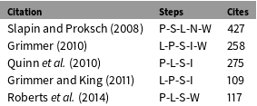
To reiterate a point we made above, whether one uses a particular preprocessing step or not should be guided by substantive knowledge. For instance, if one is working with legal data, there may be a strong a priori justification for using bigrams and trigrams such that, e.g., “Roe v. Wade” is regarded as a unified token worth counting. In practice, we observe scholars following previous work, without much theoretical basis to form an independent justification for the case at hand. And to the extent that the much emulated (see Table 1) pioneering pieces in the discipline justify their own decisions, it is typically via experiences from one set of supervised techniques that do not necessarily apply to another set—unsupervised. In the supervised case, which is relatively rare in political science applications (though see e.g. Laver, Benoit, and Garry Reference Laver, Benoit and Garry2003; Hopkins and King Reference Hopkins and King2010; Diermeier et al. Reference Diermeier, Godbout, Yu and Kaufmann2011; D’Orazio et al. Reference D’Orazio, Landis, Palmer and Schrodt2014; King, Lam, and Roberts Reference King, Lam and Roberts2017), researchers have a set of hand-labeled training documents and they wish to learn the relationship between the features (e.g. terms) those texts contain and the labels they were given.Footnote ⁵ This is helpful because it allows scholars to automatically and rapidly classify new documents into the classes they care about. By contrast, unsupervised methods—for example topic models—do not require the researcher to provide prelabeled documents. Instead, the model or technique reveals hidden structure within and between documents, and it is the job of the analyst to then interpret that information in a way that is substantively informative.

Table 1.

Preprocessing steps taken/suggested in recent notable papers that deal with unsupervised learning methods. The cite total is taken from Google Scholar at the time of writing. In the case of Slapin and Proksch (Reference Slapin and Proksch2008), we consulted their Wordfish manual (version 1.3). In the case of Roberts et al. (Reference Roberts, Stewart, Tingley, Lucas, Leder-Luis, Gadarian, Albertson and Rand2014), the authors suggest further steps might be appropriate for a given application.

In the supervised context, preprocessing—more commonly referred to as “feature selection”—is done for three primary reasons (Manning, Raghavan, and Schütze Reference Manning, Raghavan and Schütze2008; James et al. Reference James, Witten, Hastie and Tibshirani2013): first, because it reduces the size and complexity of the vocabulary which will act as input to the prediction process. This can substantially cut the computational time it takes to learn a relationship in the data for obvious reasons: for a given number of documents, learning how their class is predicted from the $10,000$ different terms they contain is likely to be slower than understanding the relationship between their class and, say, $100$ different terms. Second, preprocessing reduces the number of irrelevant (“noise”) features, the presence of which can make classification actively worse. The particular threat here is the inclusion of “unhelpful” (often rare) terms will mean that new documents will be misclassified as a product of the technique “overfitting” to such words in the training set. Thirdly, preprocessing makes models easier to interpret substantively because not only is the number of predictors reduced (mechanically lessening the workload for the researcher), but those that do remain are the more important ones for the problem at hand.

There are numerous feature selection methods in this literature, including mutual information and various $\unicode[STIX]{x1D712}^{2}$ procedures along with more elaborate regularization procedures. Regardless of the method, in the supervised context, notice that whether or not a given preprocessing step is merited can be evaluated in a well-defined way. For example, applying a given transformation to the document vectors might improve or reduce the accuracy of a classifier—literally, the proportion of cases that the learner places in the correct class. This applies similarly to other measures of classifier effectiveness, including precision, recall or $F_{1}$ score. Indeed, scholarly accounts of various areas of supervised learning include discussions of optimal feature selection on such grounds (see, e.g., Sebastiani Reference Sebastiani2002, for a comprehensive review). In given substantive domains, such work allows researchers to conclude that, for example, “bigram information does not improve performance beyond that of unigram presence”, when classifying movie reviews in terms of their sentiment (Pang, Lee, and Vaithyanathan Reference Pang, Lee and Vaithyanathan2002, 6).

The principle that one should seek to preserve what is informative while jettisoning what is redundant or irrelevant is a sensible one. But the way that this principle ought to be applied in an unsupervised setting is far from obvious.Footnote ⁶ This is because, for a start, we do not typically evaluate our unsupervised models in sharp, statistical effectiveness terms. While there are ways to determine the best fitting model from a set of candidates—for example, via a perplexity measure for topic modeling (e.g. Wallach et al. Reference Wallach, Murray, Salakhutdinov and Mimno2009)—they are predicated on, and have nothing directly to say about the merits of, a given set of preprocessing decisions which determine the precise format of the data to be fed to the algorithm. Instead, whether an unsupervised model is useful is typically a matter of determining whether the latent patterns it uncovers in otherwise complex data are interesting or substantively informative. For example, the model results might help us understand how legislators’ attention to issues varies over time (Quinn et al. Reference Quinn, Monroe, Colaresi, Crespin and Radev2010), how Senators vary in their priorities and credit claiming (Grimmer Reference Grimmer2010), how Japanese politicians increasingly focus on foreign policy (Catalinac Reference Catalinac2016) or how citizens differ in terms of the themes they emphasize in open-ended survey questions (Roberts et al. Reference Roberts, Stewart, Tingley, Lucas, Leder-Luis, Gadarian, Albertson and Rand2014). And this is not simply a matter for approaches, like topic models, that treat documents as a mixture of discrete elements or that assign texts to clusters. Indeed, unsupervised scaling models attempt to reveal latent traits or positions on a continuum without training on a subset of documents: thus, for example, Proksch and Slapin (Reference Proksch and Slapin2010) examine the changing ideological nature of German politics over time. In all cases, some form of validation is required (see Quinn et al. Reference Quinn, Monroe, Colaresi, Crespin and Radev2010, for an overview of methods); that is, scholars should carefully examine the output of their models and be sure it makes sense substantively and intuitively. But to underline the point, when undertaking such a task, there is no simple analogy to the fit statistics or effectiveness measures we mentioned above. Furthermore, specifically in the case of topic models, there is some evidence that what is deemed to be a model that fits well statistically need not be one that is easily or sensibly interpretable (Chang et al. Reference Chang, Gerrish, Wang, Boyd-graber, Blei, Bengio, Schuurmans, Lafferty, Williams and Culotta2009).

Given this ambiguity, it is not surprising that scholars use (and by implication suggest) different steps in practice. In Table 1, we report the steps taken in some notable recent papers that use unsupervised learning methods. Clearly authors do different things (and in different orders) meaning that, for example, it is hard to know a priori whether one should or should not remove stop words, or whether one should or should not remove infrequent terms. Theoretically at least, one could imagine trying multiple different specifications and verifying that the substantive inferences (their usefulness and sensibleness) one draws are similar. In practice, with 128 different transformations at a minimum, this is no easy task especially considering that various other options (such as numbers of topics) would increase the implied model space significantly and prohibitively. Of course, it might be that such choices are generally inconsequential for the conclusions we would draw from typical social science datasets. In that context, inference would be consistent across specifications, and there is neither a danger that a researcher stumbles on to a transformation that is unrepresentative nor could they deliberately manipulate their results via such choices. Sadly, as we show shortly, this is false. Before doing that, we briefly describe the data we use in the rest of the paper.

4 Description of Datasets Used in Analyses

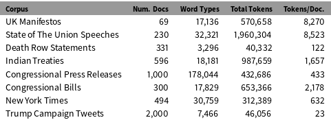
We make use of eight corpora in the analyses and examples presented in this study: they are described in Table 2, and are representative of data commonly used in the discipline.Footnote ⁷ The “UK Manifestos” are the 69 manifestos released by the Conservative, Labour and Liberal party for every general election in the United Kingdom, 1918–2001. The ‘State of the Union Speeches’ are by the President of the United States and generally given annually, 1790–2016. They can be found on numerous websites. The ‘Death Row Statements’ are transcriptions of the last words recorded by the Texas Department of Criminal Justice for 439 inmates executed by the state between 1982 and 2009. They are available on the official website of that bureau. The ‘Indian Treaties’ are historic treaties signed between the United States government and various Indian tribes between 1784 and 1911 which fall into the categories “Valid and Operable”, “Ratified Agreements”, “Rejected by Congress” and “Unratified Treaties” as described by Spirling (Reference Spirling2012). We then make use of a sample of 1,000 Senate press releases originally compiled by Grimmer (Reference Grimmer2010). The full dataset contains 72,785 press releasesFootnote ⁸ which makes it prohibitively computationally costly to preprocess 128 different ways, so we randomly selected 10 Senators, and their 100 most recent press releases as our corpus. The “Congressional Bills” are a sample of 300 bills introduced in the U.S. House of Representatives during the 113th session of Congress and originally collected by Handler et al. (Reference Handler, Denny, Wallach and O’Connor2016). The “New York Times” corpus comprises 494 articles of varying length, published between 1987 and 2007, sampled from the digital NYT archive. The Trump Campaign Tweets dataset contains 2,000 tweets written by Donald Trump between April and June 2015.Footnote ⁹

Table 2.

Corpus descriptive statistics for the five corpora used in our analyses. The number of word types, total tokens, and tokens per document were calculated using the no preprocessing specification.

5 What Could Possibly Go Wrong?

Our first claim is that while theory should guide our preprocessing choices, in practice, there is little concrete guidance for those embarking on an unsupervised analysis of a fresh dataset. Second, those choices are consequential for the inferences that can be made in terms of both substance and model fit. Here we provide evidence of these claims. In particular, we consider two small datasets and two extremely well-known and well-used techniques. We show that depending on the steps a researcher undertakes, their model results may differ in ways that could lead an honest researcher down forking paths of inference or allow a malfeasant researcher to support a range of hypotheses that may not be reflective of the universe of results.

5.1 Unsupervised scaling: An Application of wordfish

The Wordfish model of Slapin and Proksch (Reference Slapin and Proksch2008) has proved both popular and valuable for assessing the positions of parties in terms of their manifesto output, their positions in parliament (Proksch and Slapin Reference Proksch and Slapin2010) and other related matters (see, e.g., Lauderdale and Herzog Reference Lauderdale and Herzog2016, for a recent extension). Derivation and explication can be found in the original article, but it suffices to note that the core of the approach is based on a Poisson model of word use rates, with an unknown (latent) ideological position for the text (or text author) being the crucial estimand. In our current toy example, we apply the model to UK Conservative and Labour manifestos over a 15 year, four general election period: 1983, 1987, 1992, 1997. We thus have eight texts. Importantly, since this period of British history is well studied (see, e.g., Jones Reference Jones1996; Kavanagh Reference Kavanagh1997; Pugh Reference Pugh2011), we have strong priors over the relative ideological positions of at least some of the documents. Famously the “longest suicide note in history”,Footnote ¹⁰ the 1983 Labour manifesto put forward a heady and unpopular brew of unilateral nuclear disarmament, higher taxes, withdrawal from the European Economic Community and substantial (re)nationalization of industry. Meanwhile, the 1997 Labour manifesto extolled what came to be seen as the ‘third way’ position which combined social democracy with more right-wing economic policies. This was in keeping with a Labour party that had subsequently ditched ‘Clause IV’ of its constitution (formally committing it to nationalization) and clawed its way back to the center of British politics.

Taking into account reviews of Conservative positions over the same time, a reasonable observer might place the documents, left to right (with conservative documents being associated with higher latent positions), as follows:

$$\begin{eqnarray}\displaystyle \text{Lab}_{1983}<\text{Lab}_{1987}<\text{Lab}_{1992}<\text{Lab}_{1997}<\text{Con}_{1992}<\text{Con}_{1997}<\text{Con}_{1987}<\text{Con}_{1983}.\end{eqnarray}$$

In practice, we do not require readers to agree with this rank ordering to make our main point, though it will help to set expectations.

Figure 1.

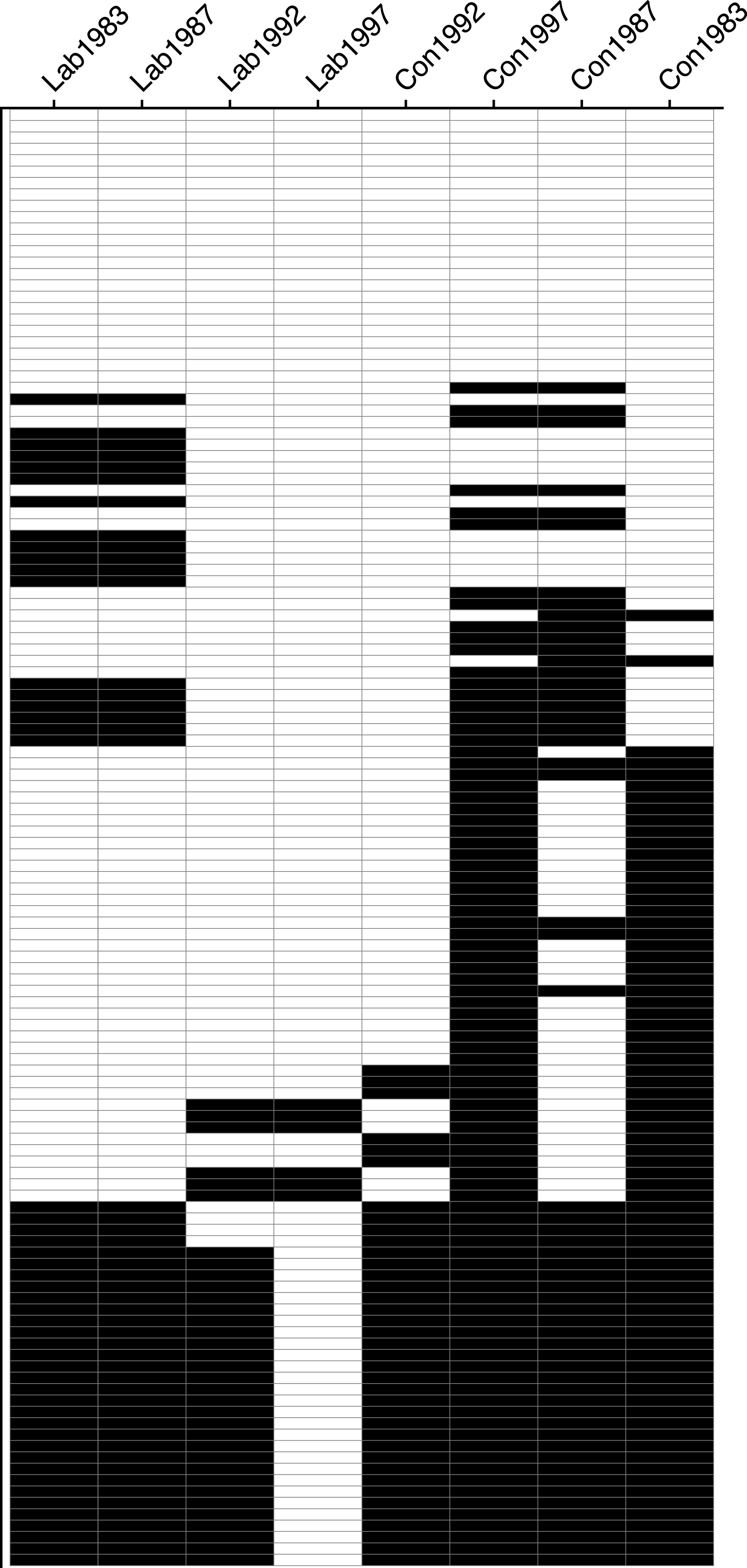
Wordfish results for the 128 different preprocessing possibilities. Each row of the plot represents a different specification. A white bar implies that the manifesto for that year is in the correct place as regards our priors. A black bar implies it was misplaced.

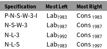
Recall that we have a total of 128 different preprocessing possibilities for the DTM, where 127 of them are something other than the original DTM for which we have undertaken no preprocessing steps. Thus, we have 128 DTMs to pass to the Wordfish software.Footnote ¹¹ Our interest here is the different rank orders the model suggests (again, in terms of the latent positions of the parties). In Figure 1 we report the results in a single plot, with 128 rows. Each row of the plot represents a different specification. A white bar implies that the manifesto for that year is in the correct place as regards our priors. A black bar implies it was misplaced. Thus, at the top of the plot we have specifications which placed the parties in the “correct” order in terms of our priors. At the bottom we have specifications which were almost completely “wrong” (no parties in the correct slot). An immediate observation is that different specifications produce different orderings. Indeed, there were a total of twelve unique orderings of the manifestos from the 128 possible preprocessing steps. Furthermore, the substantive differences between at least some of the specifications are quite stark. Consider Table 3, where we consider the “most left” and “most right” manifestos under some different specifications of the preprocessing steps. Clearly, depending on the particular choices the researcher makes, the poles of British politics move substantially: under P-N-S-W-3-I the manifestos are as expected, with Labour’s 1983 effort on the far left, and the Tory document of the same year on the far right. Meanwhile, under N-L-3, the researcher would be able to conclude that in fact Labour’s manifesto of 1992 marked the high watermark for socialism, while the Conservatives’ 1987 manifesto was the most extreme right-wing document for this period. To underline the main point here, none of these specifications are unreasonable a priori, but they yield very different conclusions. And this is true regardless of the strength of ones priors about the “correct” rank ordering. In a more cynical light, our results suggest that a malfeasant researcher could, by fitting and refitting under different specifications, support an extremely diverse array of theories. They could conclude, for example, that Michael Foot as leader in 1983 was not especially left wing, and that it was Neil Kinnock (who lead the party to election defeat in 1992) that had to go before the party was electable.

Table 3.

Some example specifications which differ in terms of the manifestos they place on the (far) left and (far) right under the Wordfish model.

5.2 Topic modeling: An application of LDA

In order to evaluate the effects of the preprocessing decisions we consider in topic modeling applications, we conducted a relatively simple experiment. We made use of the Congressional Press Releases corpus, which contains 1,000 documents written by ten different members of congress (100 each) for this experiment. For each preprocessing specification, we determined the optimal number of topics to characterize that specification using a perplexity criterion, which is discussed below. Note that we only consider the 64 specifications that do not include trigrams in this application, due to the very large computational costs associated with fitting topic models to corpora with large vocabularies. We then fit a topic model with the optimal number of topics to each DTM. Afterward, we looked at the top-twenty terms associated with each topic and picked out a series of five “key terms” that strongly anchored our interpretation of the meaning of a topic in at least one of the preprocessing specifications. We then looked for the prevalence of these key terms in topics across all specifications. We found that the proportion of topics in which they appear varies dramatically across preprocessing specifications, likely leading a practitioner to draw different substantive conclusions.

A standard metric for evaluating a particular set of parameters for a probabilistic model is to measure the log-likelihood of a held-out test set under those parameters. In the topic model context, the most commonly used metric is a normalization of the held-out log-likelihood known as perplexity—and that is what we used to determine the optimal number of topics, $k$ for a model fit to each preprocessing specification.Footnote ¹²

Figure 2.

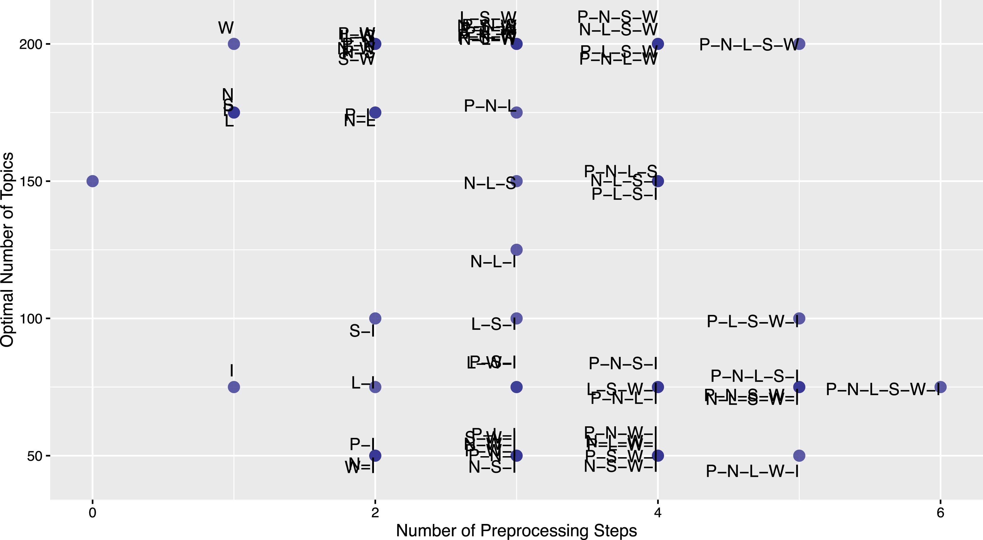
Plot depicting the optimal number of topics (as selected via perplexity) for each of 64 preprocessing specifications not including trigrams. On the x-axis is the number of preprocessing steps, and the y-axis is the number of topics. Each point is labeled according to its specification.

In particular, to determine the optimal number of topics for a given combination of steps, we conducted a grid search over $k=\{25,50,75,100,125,150,175,200\}$ topics and calculated the perplexity for each choice of $k$ using a 10-fold cross-validation procedure.Footnote ¹³ All topic models were fit using the original variational inference algorithm for LDA, as proposed by Blei, Ng, and Jordan (Reference Blei, Ng and Jordan2003). The optimal number of topics associated with each specification is depicted in Figure 2: clearly $k$ has a very large range, right across the different possibilities. Thus it as low as 50 topics in the case of P-N-L-W-I, but as high as 200 in the case of P-N-L-S-W. Similar results can be seen for N-S-I vs. L-S-W. To underline the point here: the objectively “best” topic model—by the industry standard measureFootnote ¹⁴ —varies widely and unpredictably, and depends very heavily on minor perturbations of preprocessing choices.

After determining the optimal $k$ for each preprocessing specification, we then fit a single topic model to the entire corpus (1,000 documents) for each preprocessing specification, using the optimal number of topics.Footnote ¹⁵ A common substantive analysis step after fitting a topic model is to look at the top $t$ terms associated with each topic. We chose to extract $t=20$ top terms associated with each topic, across all specifications. Examination of a sample of these topic top words across several specifications revealed some “key terms” which in our evaluation anchor a particular topic. This means that when we looked at the top-twenty words in the topic, those terms tended to provide substantial information as to what the topic is about. For example “stem” and “cell” anchor topics that relate to press releases about stem cell research, while “Iraq” anchors topics that relate to press releases about the war in Iraq. We do not claim that these are the only important terms in the results we looked at, but only that as well intentioned researchers, these terms tended to consistently and strongly influence our evaluations as to what a topic was about.

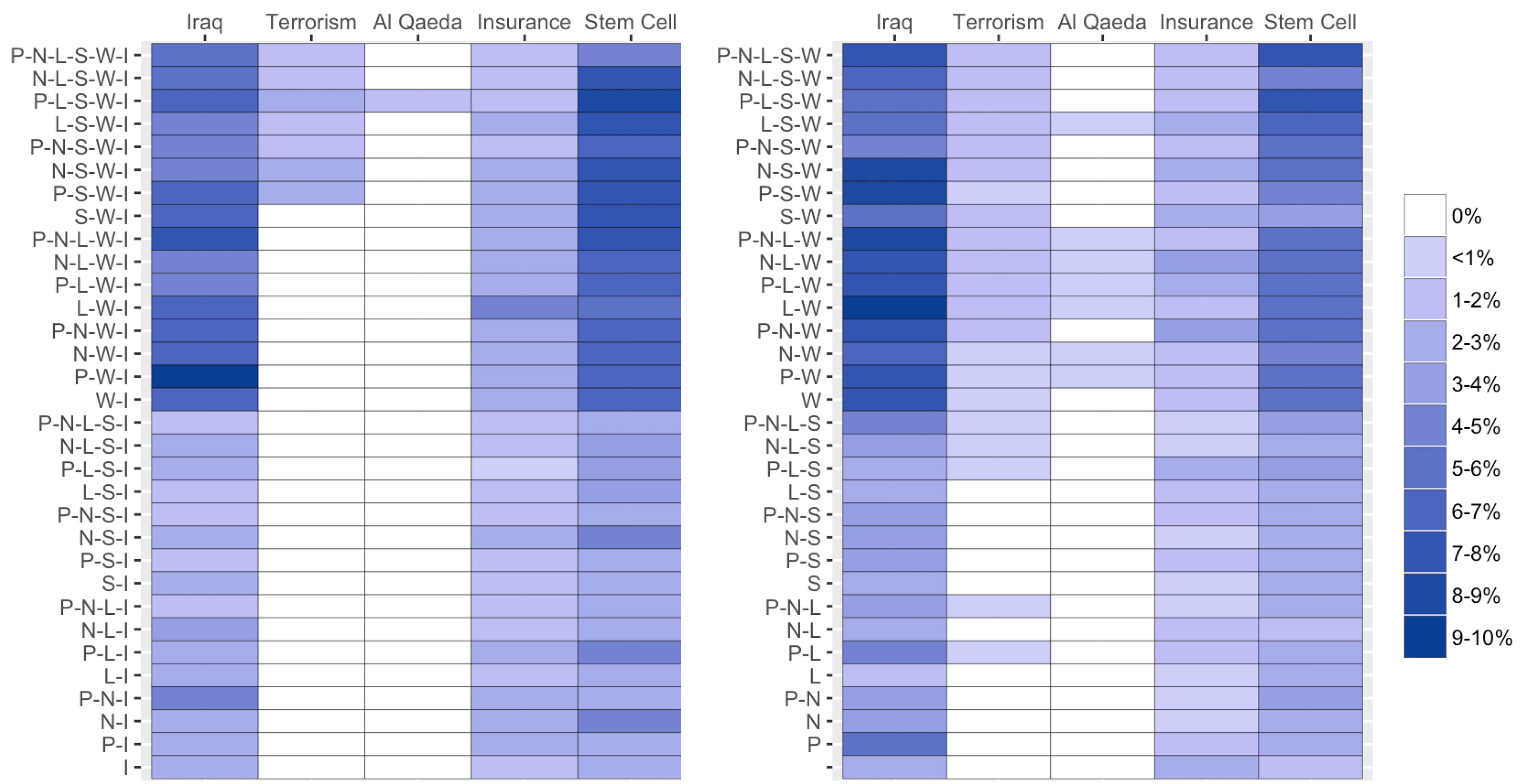
To see if these prominent anchor terms appear in topic top-twenty terms across our preprocessing specifications, we performed a case-insensitive search for the stem of each of five key terms $\{$ “iraq”, “terror”(ism), (al) “qaeda”, “insur”(ance), “stem” (cell) $\}$ in all topics across all specifications. We then calculated the proportion of topics each key word appeared in, for each specification.Footnote ¹⁶ These results are presented in Figure 3.

Figure 3.

Plots depicting the percentage of topic top-20 terms which contain the stem of each of five keywords, for each of 64 preprocessing steps (thus excluding those which include trigrams). The number of topics for specifications fit to each of the 64 DFMs were determined through tenfold cross-validation, minimizing the model perplexity.

As we can see, there is a great deal of variation in the proportion of topics each key word appeared in. To verify that this variation is not simply being driven by the instability of LDA, we replicated our analysis with forty different initializations, and the average outcomes remain strikingly similar (see Online Appendix D). These results illustrate two related issues. First, some key terms do not appear at all in the top terms for some preprocessing specifications. This means that upon inspection of the topic model results, a researcher might be unaware that there were any press releases discussing some of these key issues such as “terrorism” or “Al Qaeda”. Thus the researcher could draw different substantive conclusions about what legislators have public views on, depending on which preprocessing specification they select. Second, for some key terms such as “Iraq” or “Stem Cell”, there is about an order of magnitude difference in the proportion of topics in which a term appears, depending on the specification. This could similarly lead a researcher to different conclusions about the partisan valence or salience of these issues to members of Congress. For example, a single topic related to “stem cells” might combine together different partisan terms related to the issue in the same topic, whereas these terms might separate into several topics in an alternate specification. However, there are also some key terms (such as “insurance”) which do not exhibit the same degree of variation in their prevalence across preprocessing specifications.

To reiterate a point we alluded to above, an experienced practitioner of topic modeling might not find the results presented here especially troubling. This is because the careful use of hyperparameter optimization, asymmetric priors, or an alternate estimation method might make the results look more similar across preprocessing specifications. Furthermore, they might deliberately employ a specific set of preprocessing steps to highlight certain types of terms in topic model results. However, the vast majority of social scientists engaged in exploratory analysis of topic top terms are unlikely to be aware of the current state of the art. Our main point then remains: it is possible that a well intentioned researcher could be lead to radically different conclusions depending on how they preprocess their data.

6 preText: A New Method for Assessing Sensitivity

In the previous section, we showed that even “reasonable” preprocessing decisions can have large and unexpected consequences for both substantive inferences and the appropriate model specification for the data. In this section, we turn to ways that researchers might assess how their preprocessing decisions are likely to affect their results, and try to offer some general advice about how to proceed. As always, we would suggest that researchers should first consult theory, and our approach here is intended to complement that crucial step. Putting that point aside for now, we need to arrive at a basic metric by which to measure how different one DTM is from another.

As we noted above, researchers undertaking unsupervised analyses are typically looking to explore or describe somewhat complex datasets, and to throw (possibly hidden, latent) relationships between observations into starker relief than as they originally appear. With that in mind, we claim that what matters to researchers who are seeking to see these new patterns is how documents “move” relative to one another when they apply some transformation to the DTM, be it a topic model, scaling routine or some decomposition. One of the simplest operations a researcher can undertake—and indeed, one that forms the basis for many more complicated approaches such as principal components analysis—is to generate pairwise distances between documents. It is this very basic step that we focus on here.

To fix ideas, consider the following toy example. A researcher has three documents, $\text{doc}_{1}$ , $\text{doc}_{2}$ and $\text{doc}_{3}$ . These might be single texts, or three sets of multiple texts where each set is written by a different author. The distance, say measured in Euclidean or cosine terms, between any two of the documents indexed by $i$ and $j$ is $d(i,j)$ . When using the original DTM, for which the researcher has undertaken no preprocessing at all, the distances are $d(1,2)=1$ while $d(1,3)=3$ and $d(2,3)=2$ . So, relatively speaking, $\text{doc}_{1}$ and $\text{doc}_{3}$ are far apart. Suppose now we impose a particular preprocessing step, such as the removal of stop words and rerun our similarity analysis. On inspection we see that now, $d(1,2)=2$ while $d(1,3)=6$ and $d(2,3)=4$ . While all the distances have been doubled, the ranking of pairwise distances has remained the same: $d(1,3)>d(2,3)>d(1,2)$ . In this context, we suspect that a researcher would think these specifications are equivalent (in substance terms): things are (up to a constant) as they were previously.

By contrast, suppose that a given preprocessing step altered the distances as follows: $d(1,2)=4$ while $d(1,3)=1$ and $d(2,3)=6$ . Now, the distance between documents 2 and 3 has grown in relative terms, while $\text{doc}_{1}$ and $\text{doc}_{3}$ are more similar than previously thought. Most importantly, the order of the distances is different: $d(2,3)>d(1,2)>d(1,3)$ . This would imply a new substantive conclusion, or at least provide an opening for one.

Given that researchers in the social sciences typically do more than inspect similarities, why focus our concerns on pairwise distances? First, as we noted above, changing distances between documents have mechanical, “knock on” consequences for the data fed to a more complex technique and thus the (substantive) conclusions that may be drawn from them. Second, specifically on the issue of the importance of pairwise comparisons, we would contend that as a behavioral regularity, researchers—either implicitly or explicitly—commonly use them to validate and interpret their findings. This is because scholars typically have strong priors about (only) one or two or a few particular units, be they manifestos (e.g. Labour 1983 v Labour 1997), or Senators (Elizabeth Warren vs. Marco Rubio), or parties (Front National vs. Parti socialiste in France) in terms of where they lie in some space. If such “landmark” distances change rapidly and unpredictably between specifications of preprocessing steps, we claim that researchers would (or should!) regard this fact as concerning. For example, if removing punctuation meant that the distance between the Labour 1983 manifesto and Conservative 1983 manifesto was the largest pairwise distance observed in the DTM (something which makes substantive sense), but removing punctuation and numbers meant that this pairwise distance was the fifth largest observed (which makes little sense), red flags should be raised. Put very crudely, our logic is as follows: pairwise distance changes are not all that matters, but if they do not matter, it is not clear what does.

To begin to formalize our intuition here, consider a researcher starting with the original DTM, and considering one specification, denoted $M_{1}$ of the possible 127 preprocessing specifications we identified. They apply the specification in question and ask themselves “when I use this preprocessing step, which document pair changes the most in rank order terms?” Just assuming away ties for the moment, one pair of document must move up or down (i.e. in absolute terms) the rank order more than any other. In the running example above, $d(1,3)$ moved from third to first place in rank terms, relative to $d(2,3)$ and $d(1,2)$ . Thus $d(1,3)$ was the biggest mover. Suppose now that the researcher asks whether $d(1,3)$ is the biggest mover (again in rank order terms) when going from the original DTM to the next preprocessing option (of the 126 remaining), which we denote as $M_{2}$ . She finds that it was not: now, it is $d(2,3)$ that changes the most. Similarly, for the third possible preprocessing step $M_{3}$ (of 125 remaining) she finds that $d(2,3)$ is the biggest mover. And, in fact, for every other one of the 124 remaining preprocessing specifications $M_{3},\ldots ,M_{127}$ , the researcher finds that $d(2,3)$ moves most. What this implies is that the first preprocessing specification, $M_{1}$ , was something of an “outlier”—it moved $d(1,3)$ the most, but every other specification did not. Those other specifications favored a different pair in terms of top mover.

We can make this idea more helpful by switching the focus from pairwise distances to the specifications themselves. Again, consider $M_{1}$ and suppose there were now 6 documents in the corpus (meaning there are 15 pairwise distances). As we saw, a given specification, like $M_{1}$ , will rank a particular distance at “number 1” in absolute terms of its movement. Now consider seeing where specification $M_{2}$ ranks that largest mover from $M_{1}$ , and where $M_{3}$ ranks that largest mover from $M_{1}$ and so on through all the specifications. For 127 different specifications, we have vector of length 126 for $M_{1}$ , looking something like this

$$\begin{eqnarray}\mathbf{v}_{\mathbf{M}_{\mathbf{1}}}=(2_{M_{2}},14_{M_{3}},2_{M_{4}},3_{M_{5}},8_{M_{6}},7_{M_{7}},\ldots ,15_{M_{127}}).\end{eqnarray}$$

In this particular example, the pairwise distance most affected by $M_{1}$ was only the second most affected under $M_{2}$ (thus $2_{M_{2}}$ ) while it was the 14th most affected under $M_{3}$ (thus $14_{M_{3}}$ ), the second most affected under $M_{4}$ and so on down to the 127 specification where, in fact, that pairwise distance was the smallest mover as one went from the original DTM to $M_{127}$ . In principle, the researcher could undertake this exercise for every single one of the specifications. In the limit, a vector of ones, i.e. $\mathbf{v}_{\mathbf{M}_{\mathbf{i}}}=(1,1,\ldots ,1)$ implies that the given specification $M_{i}$ gives similar results—at least in terms of the largest pairwise distance mover—to all other specifications. By contrast, a vector of $\frac{n(n-1)}{2}$ where $n$ is the size of the corpus (in the example here, $\frac{5\cdot 6}{2}=15$ ) implies that, in terms of what it suggests is the largest mover, this specification is completely dissimilar to every other one (they rank that pair last in terms of absolute distance movement).

6.1 preText scores

Of course, it may be misleading to only look at the single pair that is induced to change most in rank order terms. A more general approach is to look at the top $k$ pairs which change the most in rank order terms. Then for each of these pairs we can calculate $\mathbf{v}_{\mathbf{M}_{\mathbf{i}}}^{(\mathbf{k})}$ —the rank difference for pair $k$ between specification $i$ and all others—and take the average of these differences across the top $k$ pairs. Doing so gives us a more general sense of the degree to which a particular preprocessing specification is unusual compared to others, as it is less likely to be affected by any one unusual document pair. One question is why not compare the rank orders of all document pairs, and the answer is primarily a practical one: this is incredibly computationally intensive, to the point where it is impractical for even moderately sized corpora. However, in practice, we have found that setting $k=50$ provides results which are stable to increasing the value of $k$ . 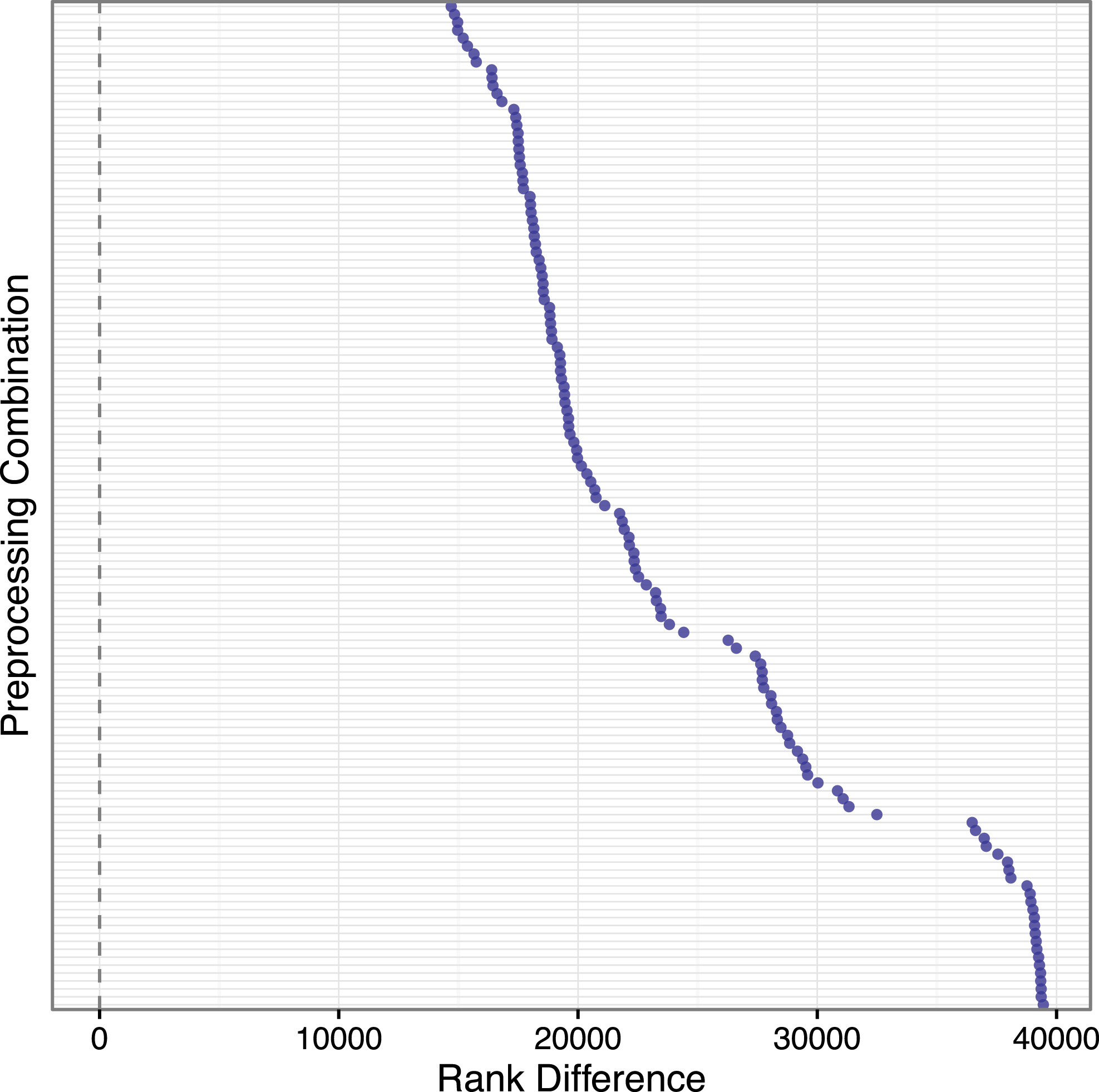As an example, we calculated the average difference in pairwise rank orderings for $k=100$ for our Indian Treaties corpus. Cosine distance was used as the underlying distance metric in this example (and all others in this study), but the results were not particularly sensitive to using Euclidean distance as an alternative measure. The results are illustrated in Figure 4, with each row on the $y$ -axis corresponding to one of the 128 choice combinations, and each point on the $x$ -axis being the mean rank difference for every one of the top-100 pairs as we move across specifications. The plot suggests that these differences can vary about threefold in magnitude.

Figure 4.

Rank test average difference results for $k=100$ for the Indian Treaties corpus ( $n=596$ ). The maximum possible rank difference for a given document pair, for this corpus, is 177,309.

In order to make these rank differences comparable across corpora (and to look for common trends), we normalize the rank differences for each preprocessing specification. This is accomplished by dividing the rank differences by the maximal possible rank difference for that corpus. For example, a preprocessing specification whose average rank difference was 17,000 in our Indian Treaties corpus would be normalized to:

(1) $$\begin{eqnarray}\frac{17,000}{177,309}\approx 0.0959\end{eqnarray}$$

because the maximal difference in rank orderings for this corpus is 177,309. We call this normalized average rank order difference the preText score $\in [0,1]$ for that particular preprocessing combination. The lower the score for a particular preprocessing specification, the more “usual” it is, while higher scores denote an “unusual” preprocessing specification.

While finding a preprocessing specification with minimal preText score for a particular corpus is a valuable diagnostic tool, we also want to understand the impact of each particular preprocessing decision conditional on all other decisions. We can do this by specifying a linear regression with the preText score for a particular preprocessing specification as the dependent variable, and dummy variables for each preprocessing decision as predictors. The parameter estimate associated with each preprocessing step will thus tell us that on average, performing that step (controlling for all other steps), has the following marginal effect on the mean movement of the preText score.

(2) $$\begin{eqnarray}\displaystyle \text{preText score}_{i} & = & \displaystyle \unicode[STIX]{x1D6FD}_{0}+\unicode[STIX]{x1D6FD}_{1}\text{Punctuation}_{i}+\unicode[STIX]{x1D6FD}_{2}\text{Numbers}_{i}+\unicode[STIX]{x1D6FD}_{3}\text{Lowercase}_{i}+\unicode[STIX]{x1D6FD}_{4}\text{Stem}_{i}\nonumber\\ \displaystyle & & \displaystyle +\,\unicode[STIX]{x1D6FD}_{5}\text{Stop Words}_{i}+\unicode[STIX]{x1D6FD}_{6}\text{N-Grams}_{i}+\unicode[STIX]{x1D6FD}_{7}\text{Infrequent Terms}_{i}+\unicode[STIX]{x1D700}_{i}.\end{eqnarray}$$

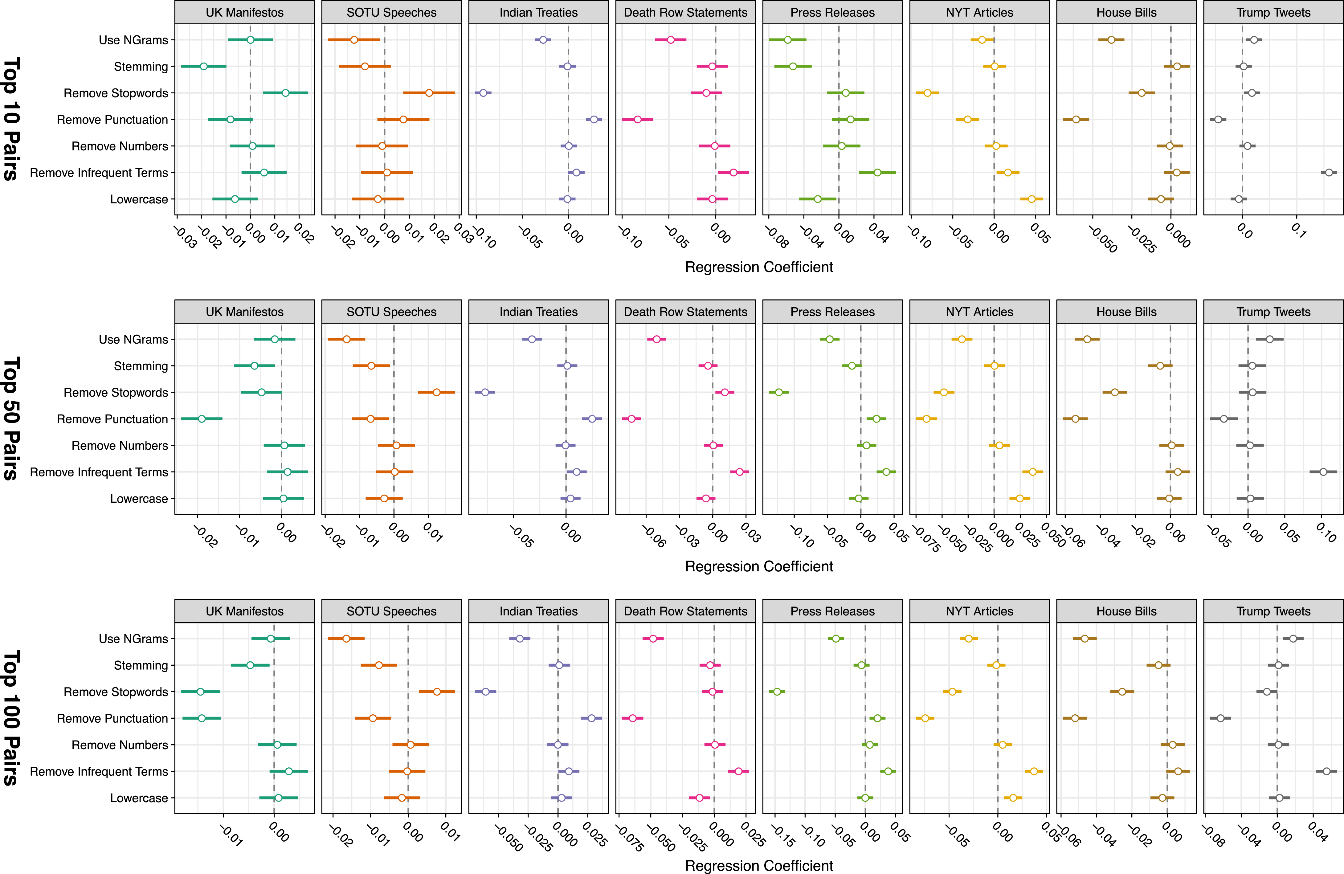
We performed this regression analysis for each of these corpora, and results are presented in Figure 5. We replicated our analysis using the top 10, 50, and 100 maximally different pairs as a basis for preText scores, in order to assess the degree to which the number of top pairs we examine affects our analysis. The $R^{2}$ for these regressions (for 100 maximally different pairs) range between 0.4 and 0.82.Footnote ¹⁷

The interpretation of these regression results is as follows: a negative parameter estimate for a particular preprocessing step for a given corpus indicates that it tends to reduce the preText score for a given specification, thus reducing the risk of drawing unusual conclusions from an analysis with that preprocessing specification applied. A positive parameter implies the opposite: that performing the preprocessing step increases the risk of drawing unusual conclusions from an analysis with that preprocessing specification applied. Just as an example, consider the fourth column of results in Figure 5, which deals with the Death Row Statements. In the first, second and third subfigure, we see that the coefficient on using $n$ -grams (“3”) is negative, as is the coefficient on removing punctuation (P), while the coefficient on removing infrequent terms (I) is positive. This implies that, for this corpus, the choices of whether to add $n$ -grams, remove punctuation, or remove infrequent terms may have a significant influence on the DTM.

More generally, for a given corpus, if all regression parameter estimates are not significantly different from zero, then any given preprocessing choice is unlikely to be overly important for the substantive conclusions drawn. Therefore, even if the researcher’s theory about which preprocessing specification is most appropriate is not particularly strong, the conclusions they draw from the analysis of their data (under their favored preprocessing specification) are not likely to be sensitive to their choice of preprocessing specification. If, however, a number of regression parameter estimates are significantly different from zero, then the conclusions they draw from the analysis of their data are likely to be particularly sensitive to their choice of preprocessing specification. In the first case, theoretical certainty about the correct preprocessing specification is less important, while in the second case, it is imperative.

Figure 5.

Regression results depicting the effects of each of the seven preprocessing steps on the preText score for that preprocessing combination.

6.2 Advice for practitioners

We suggest the following workflow for researchers seeking to draw conclusions from the analysis of DTM that are robust to their choice of preprocessing specification.

1. (1) Use theory, to the extent it exists for the problem, to choose potential preprocessing steps on the basis that the information this removes or preserves is reasonable for the application.

2. (2) Having carefully selected a theoretically motivated preprocessing specification, generate preText score regression results similar to those in Figure 5 for a random sample of up to 500–1,000 documents from the corpus. Such a sample size balances the goals of accurately approximating the entire corpus with keeping runtime under 24 hours so as not to slow down the analysis process too much.

3. (3) Examine the preText score regression results. Depending on the nature of these results and the strength of the researcher’s theory about their specification, we advocate for one of three courses of action:

   1. (a) All Parameter Estimates Are Not Significantly Different From Zero: In this case, the researcher’s conclusions are unlikely to be highly sensitive to their choice of preprocessing specification, and it is therefore reasonable to proceed with the analysis.

   2. (b) Strong Theory, Some Parameter Estimates Are Significantly Different From Zero: In this case, assess which parameter estimates are different from zero. If there is a strong theoretical reason to prefer a particular choice on each of those preprocessing steps, then (cautiously) proceed with the analysis. However, a more conservative approach would be to replicate the analysis across all combinations of preprocessing steps whose parameter estimates are significantly different from zero, and include these results as a robustness check in an appendix.

   3. (c) Weak Theory, Some Parameter Estimates Are Significantly Different From Zero: Again, assess which parameter estimates are different from zero. If there is not a strong theoretical justification for the preferred choices of these preprocessing steps, the appropriate course of action is to replicate the analysis across all combinations of preprocessing steps whose parameter estimates are significantly different from zero, and then to average or otherwise aggregate over those results in their final analysis.

Taking the steps described above may increase analysis time, but if the researcher is guided by strong theoretical expectations about the appropriate preprocessing specification for their dataset, then replication across some steps may be reasonably avoided. However, in general, the most conservative approach is simply to replicate one’s analysis across all steps with preText score regression parameters that are significantly different from zero, and include the results of those analyses as a robustness check for one’s preferred preprocessing specification.

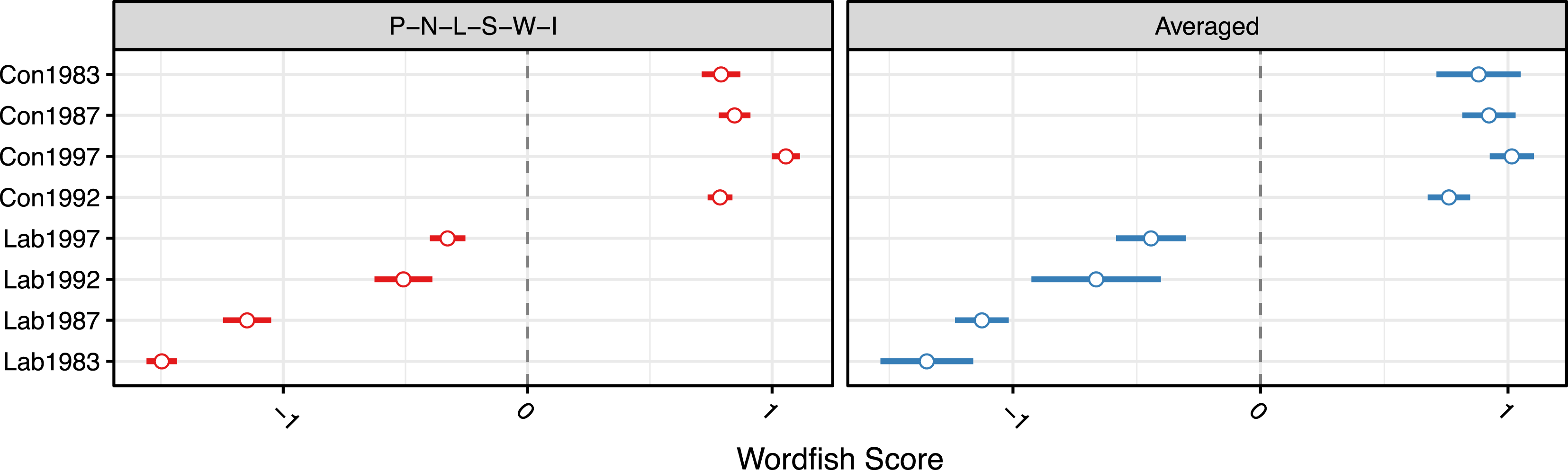
As an illustration, we apply the approach outlined above to the Wordfish example from Section 5.1. We selected a “theoretically motivated” preprocessing specification of P-N-L-S-W-I, following Grimmer and Stewart (Reference Grimmer and Stewart2013) and based on our expectations about what will and will not matter for the application. The Wordfish scores (with 95% confidence intervals) are presented in the left panel in Figure 6. Next, we averaged the Wordfish scores of eight models using every combination of the three preprocessing steps with significant parameter estimates in Figure 5: stemming (or not), stopping (or not) and removing punctuation (or not). The average Wordfish scores for these specifications, along with the appropriately adjusted 95% confidence intervals (Buckland, Burnham, and Augustin Reference Buckland, Burnham and Augustin1997), are displayed in the right panel of Figure 6.

Documents are ordered from top to bottom based on our theoretical ranking, going from most conservative to most liberal. As we can see, while both our theoretically selected and the averaged results produce the “correct” order for Labour manifestos, in both cases, Wordfish places the Conservative manifestos in the theoretically incorrect order. Looking at our theoretically selected specification (left panel), we would conclude that there is a clear ordering of:

$$\begin{eqnarray}\displaystyle \text{Con}_{1992}\sim \text{Con}_{1987}\sim \text{Con}_{1983}<\text{Con}_{1997}\end{eqnarray}$$

where $\text{Con}_{1997}$ is significantly more conservative than $\text{Con}_{1992},\text{Con}_{1987}$ or $\text{Con}_{1983}$ . However, when we incorporate the additional uncertainty from averaging across the eight possible preprocessing specifications representing the three preprocessing steps with significant parameter estimates in Figure 5, we can no longer distinguish between $\text{Con}_{1997}$ , $\text{Con}_{1987}$ and $\text{Con}_{1983}$ (right panel):

$$\begin{eqnarray}\displaystyle \text{Con}_{1992}<\text{Con}_{1997}\sim \text{Con}_{1987}\sim \text{Con}_{1983}.\end{eqnarray}$$

We note that even without model averaging we could not statistically distinguish between $\text{Con}_{1987}$ and $\text{Con}_{1983}$ . Such estimation uncertainty may mean that model averaging does not make a practical difference, in some cases. However, this can only be verified through comparison to the averaged results, so we recommend performing this procedure even when there is relatively substantial estimation uncertainty.

Coming back to our general argument, the preText score regression results for the UK manifestos provided guidance regarding which preprocessing steps to focus on in order to assess the robustness of our results in this context. By focusing on three likely consequential preprocessing decisions and averaging across those eight specifications, our results changed substantively—to be closer to the “ground truth” we identified in our example earlier.

While we believe our working example using the UK Manifestos corpus is compelling, it is reasonable to wonder whether the issues we raise are a peculiarity of the example we selected, or whether they actually effect published findings. To examine this possibility, we replicated the Wordfish analysis in Lowe and Benoit (Reference Lowe and Benoit2013) using their theoretical preprocessing specification, and model averaging implied by preText regression results. Lowe and Benoit were primarily interested in comparing human coding and Wordfish scores, but we find that it is possible to arrive at a substantively different interpretation of the Wordfish results when we use model averaging. Our replication is detailed in Online Appendix E, and we feel that it highlights the value of model averaging when the researcher does not have strong theoretical reasons for selecting a particular preprocessing specification.

Figure 6.

Wordfish scores for eight UK party manifestos generated using a theoretically selected preprocessing specification (P-N-L-S-W-I), and averaged across the eight possible DTMs generated using stemming (or not), stopping (or not) and removing punctuation (or not). These choices correspond to he choices with parameter estimates that were significantly different from zero in Figure 5.