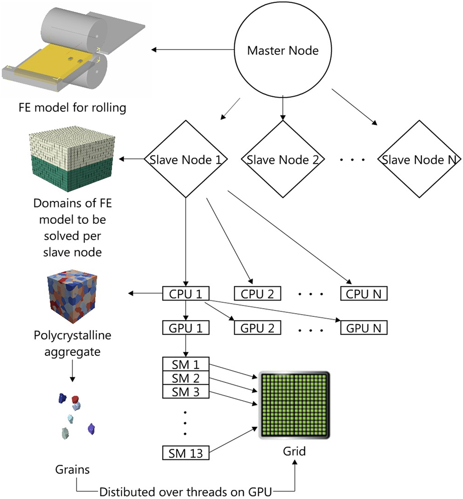
I. INTRODUCTION
Many future engineering systems will rely on advanced metals that substantially overcome the limitations of metals commonly used today. Modeling of processing–microstructure–property (PMP) relationships can aid in the manufacturing of new and advanced structural polycrystalline metals. Mechanical deformation models, in particular, can provide the microstructure–property relationship portion of the PMP when the property of interest involves evolution under mechanical strain, e.g., stress–strain response under monotonic loading, creep, fatigue, and fracture. These models can also assist in developing the processing–microstructure relationship within the PMP when the manufacturing process also involves mechanical deformation, such as in rolling or extrusions.
The central fulcrum in the PMP is microstructure—a strong suggestion that deformation models that benefit advanced structural materials design ought to incorporate the role of microstructure. During deformation processing, the microstructure changes substantially and the final microstructure is sensitive to the details of the processing, from the boundary conditions, temperature, strain rates, and sequences of deformation paths taken. During subsequent property evaluation, the microstructure significantly influences the microscopic defects, whose formation and motion accommodate deformation (dislocation glide, deformation twinning). These strong relationships have stimulated the development of microstructure-sensitive models for polycrystalline deformation over the past several decades.
Microstructure is a general term that includes a multitude of features, all of which can affect structural properties. Many of these can be considered mesoscale features: phase sizes and shape; grain size, shape, and orientation; and grain boundary and interface structure and crystallography. It remains to this day a mesoscale modeling challenge to quantitatively relate the role of so many seemingly influential microstructural features, existing at the scale of μm, in the formation and motion of the dislocations and deformation twins, operating at the scale of nm.
In this article, recent advancements in the PMP modeling of polycrystalline metals are covered. These extensions include improved ways of accounting for (i) processing boundary conditions, (ii) grain shape and texture, and (iii) grain boundaries on the chief microscopic mechanisms of deformation: slip and twinning. The insight gained in PMP relationships as a result of these modeling innovations is discussed.
The paper is organized as follows. First, the main types of mesoscale crystal plasticity-based computational techniques used to date are presented. The next part focuses on introducing various modeling advancements that lead to improved understanding of processing–microstructure relationships. These include nonhomogeneous boundary conditions and effects of grain boundaries on deformation mechanisms. The last piece of this review is dedicated to the computational needs and presentation of some promising strategies.
II. MESOSCALE METHODOLOGIES
A. Methodology overview
Structural metals are polycrystalline, or aggregates of grains, wherein each grain has a distinct crystallographic orientation with respect to all of its nearest neighboring grains.Reference Barrett and Massalski1 Many mechanics models for understanding and calculating the deformation of metals employ a combination of crystal plasticity (CP) theory and one of the various polycrystal homogenization schemes. CP theory relates the distortion of a strained crystal to slip on crystallographic slip systems.Reference Taylor2,Reference Asaro3 Polycrystal plasticity models link individual grain response predicted by CP theory to the overall mechanical response of a polycrystalline aggregate.
Polycrystal plasticity models appear in various levels of sophistication and computational efficiency. Among the more popular are polycrystal plasticity approaches, such as the full constraint Taylor model, and self-consistent schemes, such as viscoplastic self-consistent (VPSC) and elastoplastic self-consistent (EPSC),Reference Lebensohn and Tomé4–Reference Molinari, Ahzi and Kouddane8 which homogenize the neighborhood of an individual grain. Recently, self-consistent schemes have been integrated within implicit finite elements (FEs), called FE-VPSC or FE-EPSC,Reference Zecevic, Beyerlein and Knezevic9–Reference Knezevic, McCabe, Lebensohn, Tomé, Liu, Lovato and Mihaila13 wherein the material at integration points is modeled as polycrystalline aggregates and the constitutive response is provided by the SC scheme. Used less often are CP models that spatially resolve the grain neighborhoods, which can be referred to as 3D full field, spatially resolved mechanics techniques. Two examples of models in this class are CPFE modelsReference Bronkhorst, Kalidindi and Anand14,Reference Bronkhorst, Kalidindi and Anand15 and Green’s function fast Fourier transform (FFT) models.Reference Lebensohn, Liu and Ponte Castañeda16–Reference Lebensohn, Rollett and Suquet19 These can be differentiated by their solution technique.
The above CP-based models can (i) calculate and relate the evolution in the crystallographic orientation of the grains (called texture) to the overall polycrystal stress–strain response, and apart from the Taylor model, (ii) predict the evolution in the individual shape of the grains. The crystal plasticity finite element (CPFE) and CP-FFT methodologies have the ability to additionally provide nonuniform deformation fields generated in the crystals (intergranular) and between the constituent grains (intragranular).
The remainder of this article will present examples that utilize one or a combination of the mesoscale methods: polycrystal modeling, CPFE, and CP-FFT. Additionally, in one example the polycrystal models will be embedded at FE integration points, where the intrinsic homogenization constrains are relaxed. An abbreviated review of the formulation of the three CP techniques is provided in turn below. Regarding notation, vector and tensors are indicated by boldfaced characters and are not italicized. For a second-order tensor A, the notation AT denotes its transpose, i.e.,  $A_{ij}^{\rm{T}} = {A_{ji}}$ for i, j = 1, …, 3. The notation trA means its trace, while detA signifies its determinant. The contracted product between two tensors, A and B, is defined as: A·B. The dyadic product of any two vectors, a and b, is a second-rank tensor given by a ⊗ b = a ib j. Scalars and tensor components are italicized and not boldfaced.
B. Mean-field polycrystal models
The two polycrystal mean-field schemes that have been used most often for modeling polycrystalline deformation are VPSC and EPSC. In VPSC, the formulation does not include deformation by elastic deformation, but in EPSC, both elastic and plastic deformation are taken into account. In these self-consistent frameworks, the formulation relates the effective or polycrystal aggregate response with the response of individual grains. The polycrystal is represented as a collection of crystals, wherein each crystal has a specific orientation, ellipsoidal shape, and volume fraction. These model crystals do not necessarily represent specific single crystals in a microstructure, but rather as representative orientations (ROs) whose response is an ensemble average over all similarly oriented crystals in the polycrystal. In these mean-field techniques, the polycrystal is treated as a 3D homogeneous continuum. Topologically, information of, say, the specific grain neighbors or grain boundaries are not included in the solution.
In both SC models, to calculate the stress and strain response of each RO within the polycrystal, Eshelby’s solution for a 3D inclusion embedded within a continuum is used. As mentioned, the continuum is the polycrystal and commonly referred to as the homogeneous equivalent medium (HEM). An iterative scheme is used to calculate the properties of the HEM, i.e., the polycrystal, by enforcing that its properties equal the average properties of all its constituent crystals, which gives rise to the name “self-consistent”. In VPSC, the constitutive response of the ROs and HEM is “viscoplastic”. Elastic deformation is not taken into account. Thus, grain rotations result from plastic spins but not elastic spins. In elastic–plastic self-consistent EPSC, the grains and polycrystal deform by elastic deformation as well as by crystallographic slip. The plastic response in both schemes is calculated using CP, wherein slip and twinning occur on specified crystallographic systems. Grain rotations are the result of elastic and plastic spins. With this basic formulation, these SC models can predict the relationships between crystallographic texture evolution, effective stress–strain response, and the activity of the various slip/twin systems used by each grain in the polycrystal.
1. Viscoplastic self-consistent
In VPSC, both the polycrystal (medium) and each grain (ellipsoidal inclusion) are viscoplastic. Linearization of the viscoplastic constitutive response is needed to guarantee that the stress and strain rates are uniform within the Eshelby ellipsoidal domain. In linearized form, the relationship between the grain strain rate and the grain stress is given by
 $${{\dot{\boldvarepsilon }}}{_{ij}^c_{}} = {M_{ijkl}}\left( {{{{\boldsigma }}^c}} \right)\sigma _{ij}^c + \dot{\varepsilon }_{ij}^0\quad ,$$
where M ijkl and  $\dot{\varepsilon }_{ij}^0$ are the viscoplastic compliance and the back-extrapolated rate of the grain, respectively. The plastic strain rate is defined as the sum of shear strain rates,
 ${\dot{\gamma }^s}$, from each slip system, s:
 $${{{\dot{\boldvarepsilon }}}^c} = {\dot{\gamma }_0}\sum\limits_s {{{\bf{m}}^s}{{\dot{\gamma }}^s}} = {\dot{\gamma }_0}\sum\limits_s {{{\bf{m}}^s}} {\left( {\left| {{{{{\bf{m}}^s} \cdot {{\bf{\boldsigma }}^c}} \over {\tau _0^s}}} \right|} \right)^n}{\mathop{\rm sgn}} \left( {{{\bf{m}}^s} \cdot {{{\boldsigma }}^c}} \right)\quad ,$$
where  ${\dot{\gamma }^s}$,
 $\tau _0^s$, and ms are, respectively, the shear rate, the critical resolved shear stress (CRSS), and the Schmid tensor, for the slip system s. The Schmid tensor is given by ms = (bs ⊗ ns + ns ⊗ bs)/2, where bs and ns are the orthonormal unit vectors for the slip direction and slip plane normal. Parameter
 ${\dot{\gamma }_0}$ is a reference strain rate and n is the power-law exponent representing the inverse of the material rate-sensitivity.
Assuming an analogous linear relation at the macroscopic polycrystal level and performing the homogenization, the linearized relationship between the effective medium (polycrystal) strain rate and the effective medium stress becomes
 $${\overline {\dot{\varepsilon }} _{ij}} = {\bar{M}_{ijkl}}\left( {{{\bar{\boldsigma }}}} \right){\bar{\sigma }_{kl}} + \overline {\dot{\varepsilon }} _{ij}^0\quad ,$$
where  ${\overline {\dot{\varepsilon }} _{ij}}$ and
 ${\bar{\sigma }_{kl}}$ are the HEM strain rate and stress, and
 ${\bar{M}_{ijkl}}$ and
 ${\bar{\sigma }_{kl}}$ are the HEM viscoplastic compliance and back extrapolated rate, respectively. Solving the stress equilibrium equation of an ellipsoidal inclusion, described by Eq. (1.2), embedded in a homogeneous medium, described by Eq. (1.3), leads to an interaction equation relating the HEM and inclusion strain rates and stress
 $$\left( {{{\dot{\varepsilon }}_{ij}} - {{\overline {\dot{\varepsilon }} }_{ij}}} \right) = - {\tilde{M}_{ijkl}}\left( {{\sigma _{kl}} - {{\bar{\sigma }}_{kl}}} \right)\quad ,$$
where
 $${\tilde{M}_{ijkl}} = \left( {I - S} \right)_{ijmn}^{ - 1}{S_{mnpq}}{\bar{M}_{pqkl}}\quad ,$$
is the “interaction tensor” and S is the Eshelby tensor. The macroscopic moduli are unknown a priori and need to be adjusted self-consistently, by enforcing the condition that the average stress and strain rate over all inclusions has to be equal to the HEM stress and strain rate, i.e.,
 $${\overline {\dot{\varepsilon }} _{ij}} = \left\langle {{{\dot{\varepsilon }}_{ij}}} \right\rangle \;{\rm{and}}\;{\bar{\sigma }_{ij}} = \left\langle {{\sigma _{ij}}} \right\rangle \quad .$$
Substituting Eqs. (1.3)–(1.5) into Eq. (1.6) leads to an expression for the viscoplastic moduli of the linearized HEM, given by
 $${\bf{M}} = \left\langle {{\bf{MB}}} \right\rangle {\left\langle {\bf{B}} \right\rangle ^{ - 1}}\quad ,$$
 $${{{\dot{\boldvarepsilon }}}^0} = {\bf{Mb}} + {{{\dot{\boldvarepsilon }}}^0} - \left\langle {{\bf{MB}}} \right\rangle {\left\langle {\bf{B}} \right\rangle ^{ - 1}}\left\langle {\bf{b}} \right\rangle \quad ,$$
where the localization tensors are defined as
 $${B_{ijkl}} = \left( {M + \tilde{M}} \right)_{ijmn}^{ - 1}{\left( {\bar{M} + \tilde{M}} \right)_{mnkl}}\quad ,$$
 $${b_{ij}} = \left( {M + \tilde{M}} \right)_{ijmn}^{ - 1}{\left( {{{\overline {\dot{\varepsilon }} }^0} + {{\dot{\varepsilon }}^0}} \right)_{mn}}\quad .$$
The plastic rotation rate, Wp,c , of each crystal inclusion (or grain) is related to the shear rates  ${\dot{\gamma }^s}$ on the individual slip systems via the following kinematic formula:
 $${{\bf{W}}^{p,c}} = \sum\limits_s {{{\bf{q}}^{c,s}}{{\dot{\gamma }}^{c,s}}} \quad ,$$
where qc,s = 0.5(bc,s ⊗ nc,s − nc,s ⊗ bc,s ). The lattice rotation rate Wc, used to update the crystal orientation and hence calculate texture evolution, is the difference between the rotation rate due to slip and the macroscopically applied rotation rate of the grain shape Wapp,
 $${{\bf{W}}^c} = {{\bf{W}}^{p,c}} + {{\bf{\Pi }}^c} - {{\bf{W}}^{{\rm{app}}}}\quad ,$$
where Πc is the antisymmetric part of the Eshelby tensor for grain c.Reference Lebensohn and Tomé4
With the above formulation, for each strain increment, VPSC calculates a homogeneous stress state in each grain inclusion, σij, which deviates from the macroscopic stress state. The properties and response of the HEM and of the individual grains are computed in an iterative manner. Numerical integration is implicit. As is customary, the time step is selected such that the stress–strain response is independent of time step. The time step that satisfies this criterion is typically 1 × 10⁻³ s. The stress σij will be strongly dependent on the crystallographic orientation, grain shape, deformation (hardening) history, and the interaction with the surrounding HEM. Above is an abbreviated form and a complete description of the VPSC framework can be found in Refs. Reference Lebensohn and Tomé4–Reference Lebensohn, Tomé and Castaneda6.
2. EPSC
The polycrystalline EPSC model formulation was originally developed in Ref. Reference Turner and Tomé20 and in later extensions.Reference Zecevic, Beyerlein and Knezevic9,Reference Zecevic and Knezevic10,Reference Zecevic, Knezevic, Beyerlein and Tomé21 As mentioned, unlike VPSC, the EPSC polycrystal model accounts for elastic anisotropy in addition to plastic slip according to CP theory.
The macroscopic (Jaumann) stress rate and strain rate are linked through the following linear relationship:
 $${{\hat{\boldsigma }}} = {{\bf L \dot{\boldvarepsilon }}}\quad ,$$
where L is the instantaneous elastoplastic stiffness tensor of the polycrystal, which at the outset is unknown and must be solved iteratively through the standard self-consistent procedureReference Turner and Tomé20 until equilibrium and strain compatibility are satisfied.Reference Eshelby22
The strain rate in the individual inclusions (denoted by superscript c) is related to the macroscopic strain rate via
 $${{{\dot{\boldvarepsilon }}}^c} = {{\bf{A}}^c}{{\dot{\boldvarepsilon }}}\quad ,$$
where
 $${{\bf{A}}^c} = {\left( {{{\bf{L}}^c} + {{\bf{L}}^{{c^ * }}}} \right)^{ - 1}}\left( {{{\bf{L}}^{{c^ * }}} + {\bf{L}}} \right)$$
is the localization tensor for elasto-plastic ellipsoidal inclusion, Lc is the instantaneous elasto-plastic stiffness tensor, and
 $${{\bf{L}}^{{c^ * }}} = {\bf{L}}\left( {{{\bf{S}}^{{c^{ - 1}}}} - {\bf{I}}} \right)$$
is the effective stiffness tensor for the inclusion and Sc is the symmetric Eshelby tensor for the inclusion c, and I is the fourth rank identity matrix. This tensor Lc* relates the stress and total strain rate in a grain to the stress and total strain rate in the HEM through an interaction equation, given by
 $$\left( {{{{{\hat{\boldsigma }}}}^c} - {{\hat{\boldsigma }}}} \right) = - {{\bf{L}}^{{c^ * }}}\left( {{{{{\dot{\boldvarepsilon }}}}^c} - {{\dot{\boldvarepsilon }}}} \right)\quad .$$
Next, the following condition that the HEM stress and strain rate is equal to the volume average of the stress and strain rate in the inclusions is enforced, i.e.,
 $${{\hat{\boldsigma }}} = \left\langle {{{{{\hat{\boldsigma }}}}^c}} \right\rangle \quad ,$$
and
 $${{\dot{\boldvarepsilon }}} = \left\langle {{{{{\dot{\boldvarepsilon }}}}^c}} \right\rangle \quad ,$$
which provides an expression for L:
 $${\bf{L}} = \left\langle {{{\bf{L}}^c}{{\bf{A}}^c}} \right\rangle {\left\langle {{{\bf{A}}^c}} \right\rangle ^{ - 1}}\quad .$$
To calculate the macroscopic Cauchy stress, the following relationship between the Cauchy stress rate and Jaumann rate is used:
 $${{\dot{\boldsigma }}} = {{\hat{\boldsigma }}} + \left\langle {{{\bf{W}}^c}{{{\boldsigma }}^c}} \right\rangle - \left\langle {{{\bf{\boldsigma }}^c}{{\bf{W}}^c}} \right\rangle = {{L\dot{\boldvarepsilon }}} + \left\langle {{{\bf{W}}^c}{{{\boldsigma }}^c}} \right\rangle - \left\langle {{{{\boldsigma }}^c}{{\bf{W}}^c}} \right\rangle \quad ,$$
where Wc is the lattice spin given by Eq. (1.12).
The above relationship is integrated explicitly over time, i.e.,  ${{{\boldsigma }}_{n + 1}} = {{{\boldsigma }}_n} + {{\bf{L}}_n}{{{\dot{\boldvarepsilon }}}_n}\Delta t + \left\langle {{\bf{W}}_n^c{{\boldsigma }}_n^c} \right\rangle \Delta t - \left\langle {{{\boldsigma }}_n^c{\bf{W}}_n^c} \right\rangle \Delta t$. With the remaining field variables, such as the elastic spin and strain rate at the current increment n, the HEM stress can be updated for the next increment n + 1. The time step is selected such that the stress–strain response becomes independent of the time step. For most EPSC calculations reported in the literature, the time step is 1 × 10⁻³ s.
Finally, the constitutive relationship at the individual inclusion level between the Jaumann stress rate,  ${{{\hat{\boldsigma }}}^c}$, and the strain rate,
 ${{\bf{\dot{\varepsilon }}}^c}$, is given by
 $${{{\hat{\boldsigma }}}^c} = {{\bf{C}}^c}\left( {{{{{\dot{\boldvarepsilon }}}}^c} - {{{{\dot{\boldvarepsilon }}}}^p}} \right) - {{\bf{\boldsigma }}^c}{\rm{tr}}\left( {{{{{\dot{\boldvarepsilon }}}}^c}} \right)\quad ,$$
where Cc is the single crystal elastic stiffness tensor and as defined before in Eq. (1.2),  ${{{\dot{\boldvarepsilon }}}^p} = \sum\limits_s {{{\bf{m}}^{c,s}}{{\dot{\gamma }}^{c,s}}}$ is the plastic strain rate. To account for changes in bc,s and nc,s , the slip directions and slip planes, due to changes in crystallographic orientation as the texture evolves, the elastic stiffness is calculated at the beginning of each deformation increment.
At this point, we have reviewed two self-consistent formulations, EPSC and VPSC, and thus one question that may arise is whether the results from these two models would differ. We do not know of any formal comparisons made between the results from stress–strain and texture calculations of VPSC and EPSC. The key difference between the two formulations is that EPSC accounts for elastic deformation while VPSC does not. However as is customary in elastic–plastic constitutive models, EPSC assumes that the elastic and plastic deformations are decoupled. As a result, when EPSC and VPSC attempt to capture the same experimental plastic flow stress–strain response, the hardening parameters in the plastic part should, in principle, not be different. Any slight differences could be observed due to finite kinematics of VPSC versus small-strain kinematics of EPSC. Texture predictions should also not be appreciably different because the same kinematics is involved. The elastic deformation gradient in EPSC can be related to the kinematics used in texture evolution calculations of VPSC and EPSC.
3. Deformation twinning in mean-field codes
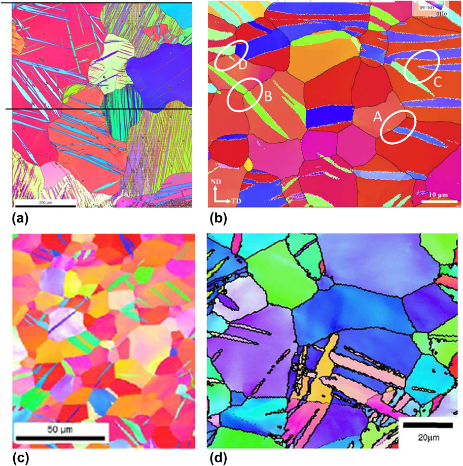
During the processing of polycrystalline metals, another stress-driven deformation mechanism that occurs often is deformation twinning. Twins are microstructural heterogeneities that reorient and shear the lattice. As a result, they form a boundary with the surrounding crystal and introduce local stress fields. Twin domains initiate as atomic-scale embryos and grow to the size of the grain, becoming mesoscale heterogeneities.Reference Beyerlein, Zhang and Misra23 Grain boundaries hinder but do not prevent the propagation of twins into neighboring grains.Reference Arul Kumar, Beyerlein, McCabe and Tomé24 Figure 1 shows examples of twins that have formed in polycrystalline materials as a result of deformation. As shown, most twins have their boundaries intersecting with grain boundaries, and in many cases, the twin is connected with another twin across the boundary.
EBSD images of deformation twins in (a) α-uranium, (b) AZ31 Mg alloy, (c) Zr, and (d) commercially pure Ti. Reprinted with permission from Ref. Reference Knezevic, Daymond and Beyerlein139.

The VPSC and EPSC models were originally developed to account only for the shear provided by twinning. Later computationally efficient methods for treating the reorientation that accompanies twinning were developed for these self-consistent schemes. These include the predominant twin reorientation (PTR) method,Reference Van Houtte25,Reference Tomé, Lebensohn and Kocks26 volume fraction transfer scheme,Reference Tomé, Lebensohn and Kocks26 total Lagrangian approach,Reference Wu, Kalidindi, Necker and Salem27 and composite-grain (CG) method.Reference Proust, Tomé and Kaschner28,Reference Mareau and Daymond29
In these schemes, the twin phase replaces some fraction of the matrix phase and as the volume of the twin phase increases with strain, the volume of the matrix phase shrinks accordingly. They generally involve splitting the original orientation (grain) into two parts, one part is twinned and another part, i.e., the matrix, while preserving the original volume fraction of the grain. As an example, we describe the CG model, which is rising to be the standard one used in VPSC and EPSC models. It was first introduced in Refs. Reference Proust, Tomé and Kaschner28 and Reference Proust, Tomé, Jain and Agnew30 and has an advantage of accounting for both morphological changes and crystallographic reorientation. In the CG model, a twinned grain is assumed to contain n uniformly spaced lamellae of equal thickness that are reoriented to twin orientation. One can choose to treat the CG grain as a single laminated inclusion in which continuity of stresses and strains at the matrix-twin boundary is enforced. Alternatively, one can treat the twinned grain as two separate inclusions that are decoupled mechanically. In this case, the simulation keeps track of the shape and orientation of the ellipsoids representing the twin and matrix and their evolving volume fractions. This information ensures that (i) as the twins thicken, the matrix regions narrow, (ii) the number of twins n in the grain and grain diameter d g limit the thickness that an individual twin can grow, and (iii) a twin spacing can be obtained, as in the case of the fully laminated grain. The newly formed twin inclusions are treated as new ellipsoidal inclusions and added to the total number of ROs in the polycrystal. As grains in these models are represented as ellipsoidal inclusions, the new twin inclusions can be initially assigned as flat ellipsoids with their short axis perpendicular to the twinning plane, to reflect the lamellar shape of newly formed twins (see Fig. 1). The twinned inclusion adopts a mirror orientation with respect to the orientation of the parent grain that is characteristic of the type of twin.Reference Beyerlein, Zhang and Misra23,Reference Christian and Mahajan31
The volume fraction of the twin increases with twin shear activity. The shear deformation provided by twinning Δγtw is localized into the twin inclusion. Because twins provide a characteristic shear per unit volume, the increment in twin volume fraction and increment in shear are related following
 $$\Delta {f^{{\rm{tw}}}} = {{\Delta {\gamma ^{{\rm{tw}}}}} \over {{S^{{\rm{tw}}}}}}\quad ,$$
where Δγtw is the shear strain contributed by the twinning system in the grain and S is the characteristic twin shear of the twin. Since the total volume fraction of the original grain does not change, as the volume fraction of the twin increases, the volume fraction of the corresponding parent grain is reduced by the same amount. With such sub-grain twinning models, mean-field polycrystal models have been successful in demonstrating many key effects of twins on the macroscopic stress–strain response and texture evolution.Reference Proust, Tomé and Kaschner28,Reference Proust, Tomé, Jain and Agnew30,Reference Capolungo, Beyerlein, Kaschner and Tomé32,Reference Proust, Kaschner, Beyerlein, Clausen, Brown, McCabe and Tomé33
Last, when the grain twins, twin boundaries will be created, which in turn can represent barriers to slip. When the CG model is implemented into either EPSC or VPSC, the evolution of the mean-free-paths d ss′ for slip in the matrix and twin domains are calculated based on the current shape of the lamella in the CG model and used in the hardening law via a directional Hall–Petch term:
 $$\tau _{{\rm{HP}}}^{\alpha \beta } = {{{H^{\alpha \beta }}\mu {b^\alpha }} \over {\sqrt {{d^{ss'}}} }}\quad s \in \alpha ,\;s' \in \beta \quad ,$$
where H αβ is the Hall–Petch coefficient. The separation distance d ss′ is defined along the slip plane of system s between two adjacent boundaries of twin system s′. Accordingly slip occurring in planes parallel to the twin-matrix interface will not experience a barrier effect posed by this boundary while slip occurring on planes that intersect the interface will. Equation (1.24) represents a “dynamic Hall–Petch effect”. As the twins thicken, the matrix regions shrink and hence, the mean free path for slip in the matrix becomes increasingly confined, while that for slip in the twin becomes easier. This concept has been implemented in a number of polycrystal models.Reference De Cooman, Estrin and Kim34–Reference Niezgoda, Kanjarla, Beyerlein and Tomé36
The coefficient H αβ in Eq. (1.24) will be particular to the hcp material and slip and twin system involved. For some combinations, for instance, this effect is negligible and H αβ accordingly is zero. Generally, not much significance can be placed in the fitted values of H αβ, as the underlying physics of slip–twin interactions has yet to be clarified.
C. CPFE
As mentioned, one 3D spatially resolved scheme used frequently in mechanical deformation modeling is the CPFE method. This technique can provide predictions of not only texture evolution but also evolution of intragrain and intergrain misorientations, grain shape, and grain boundary character distribution. Recent years have seen a rapid increase in the 3D CPFE formulation for the study of a wide variety of problems.Reference Liu, Raabe, Roters, Eisenlohr and Lebensohn18,Reference Abdolvand and Daymond37–Reference Zhang, Karimpour, Balint and Lin46
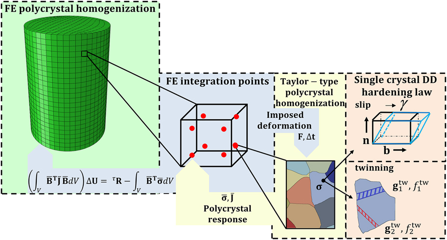
Figure 2 displays a multiscale CPFE model and the submodel components that it links. Going from left to the right side, the material length increases and each frame represents a specific instance at which the material response is being evaluated. At the coarsest level is the material response of a polycrystal, which is in the form of a granular microstructural model, by the use of the FE homogenization method. As a full-field model, this method fulfills both stress equilibrium and strain compatibility conditions making it a suitable modeling tool for capturing the interactions between the constituent grains. Each grain in the polycrystal is represented by an element set, which discretizes a given grain into FEs. At this length scale, at each FE integration point, the material constitutive response is being estimated utilizing CP theory. The FE integration point can embed a single crystal or a polycrystal. The later requires a homogenization like Taylor-type or self-consistent. In application of CP, the model usually allows the strain to be accommodated by the simultaneous action of crystallographic slip and deformation twinning. In CPFE, the shear accommodated by the latter mechanism is most often modeled as slip and is referred to as the pseudo slip model for twinning.Reference Van Houtte25,Reference Kalidindi47
A multiscale modeling framework for the plastic deformation of polycrystals. Reprinted with permission from Ref. Reference Ardeljan, Beyerlein, McWilliams and Knezevic40.
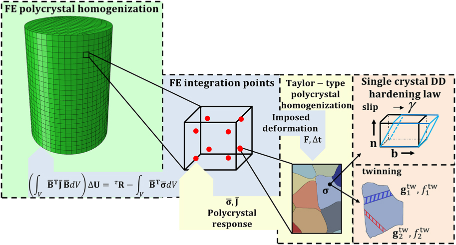
To determine the single crystal response at each integration point, a User MATerial subroutine based on CP constitutive formulation is used in Abaqus Standard. The framework facilitates various loading conditions from low to high level of complexity that can be applied in the form of suitable boundary conditions. This applied load is divided into time/strain increments, where for each and every a global stress equilibrium solution is found using a numerically iterative procedure of the FE method. This end is achieved by solving the nonlinear FE governing equation in its linearized form given by
 $$\left( {\int_V {{{\bf{B}}^{\rm{T}}}{\bf{JB}}{\rm{d}}V} } \right)\Delta {\bf{U}} = {\bf{R}} - \int_V {{{\bf{B}}^{\rm{T}}}{\bf{\boldsigma }}{\rm{d}}V} \quad .$$
In this relation, the listed quantities are, respectively, B—FE strain-displacement matrix, J—material Jacobian matrix, ΔU—displacement increment solution, R—applied force vector, and σ—Cauchy stress tensor.Reference Zecevic, Beyerlein and Knezevic9,Reference Bathe48,Reference Zecevic, McCabe and Knezevic49
An essential part of CPFE is the CP constitutive law that relates the material stress to material distortion (stretch plus rotation) at each integration point within each FE in the model.Reference Kalidindi, Bronkhorst and Anand50,Reference Kalidindi, Duvvuru and Knezevic51 The description of the law that follows adopts standard continuum mechanics notation, where tensors are denoted using roman boldface symbols, while scalars are italicized and not boldfaced. To denote a time derivative, a dot is placed over a particular quantity.
The total velocity gradient tensor, L, can be additively decomposed as follows:
 $${\bf{L}} = {{\bf{L}}^{\rm{e}}} + {{\bf{L}}^{\rm{p}}}\quad ,$$
where Le and Lp represent elastic and plastic velocity gradients, respectively. The plastic part of the velocity gradient contains the contributions from both slip and twinning via
 $${{\bf{L}}^{\rm{p}}} = {{\bf{L}}^{{\rm{sl}}}} + {{\bf{L}}^{{\rm{tw}}}}\quad .$$
The corresponding contributions to the velocity gradients, due to slip and twinning, are further expressed as
 $${{\bf{L}}^{{\rm{sl}}}} = \sum\limits_\alpha ^{{N^{{\rm{sl}}}}} {{{\dot{\gamma }}^\alpha }{\bf{m}}_{\rm{o}}^\alpha } = \sum\limits_\alpha ^{{N^{{\rm{sl}}}}} {{{\dot{\gamma }}^\alpha }{\bf{b}}_{\rm{o}}^\alpha \otimes {\bf{n}}_{\rm{o}}^\alpha } \quad ,$$
 $${{\bf{L}}^{{\rm{tw}}}} = \sum\limits_\beta ^{{N^{{\rm{tw}}}}} {{{\dot{f}}^\beta }{S^\beta }{\bf{m}}_{\rm{o}}^\beta } = \sum\limits_\beta ^{{N^{{\rm{tw}}}}} {{{\dot{f}}^\beta }{S^\beta }{\bf{b}}_{\rm{o}}^\beta \otimes {\bf{n}}_{\rm{o}}^\beta } \quad ,$$
where  ${\dot{\gamma }^\alpha }$ stands for the shearing rate on the slip system α,
 ${\bf{m}}_{\rm{o}}^\alpha$ and
 ${\bf{m}}_{\rm{o}}^\beta$ are the Schmid tensors associated with slip system α and twin system β, respectively, and S β is the characteristic twin shear for the twin system β. Finally, N sl and N tw represent the total number of available slip and twinning systems, respectively. The Schmid tensors represent the unit slip or twin system tensor, defined as the dyadic product (⊗) between the unit Burgers direction (bo) and unit plane normal (no) vectors of slip system α or twin system β, respectively, in the undeformed configuration indicated by subscript ‘o’. The rate of change of the twin volume fraction per twin system
 $\left( {{{\dot{f}}^\beta }} \right)$ is related to the shear rate on the twin system
 $\left( {{{\dot{\gamma }}^\beta }} \right)$ according to Refs. Reference Van Houtte25 and Reference Kalidindi47:
 $${\dot{f}^\beta } = {{{{\dot{\gamma }}^\beta }} \over {{S^\beta }}}\quad .$$
In the finite deformation formulation, an assumption is made that the deformation gradient (F) can be multiplicatively decomposed into its elastic (Fe) and plastic (Fp) contributions according to
 $${\bf{F}} = {{\bf{F}}^{\rm{e}}}{{\bf{F}}^{\rm{p}}}\quad ,$$
where the elastic component contains contributions from both elastic stretching and lattice rotation, while the plastic component embodies contributions due to plastic deformation. The constitutive relationship between Fe and stress in the crystal is given by the two expressions for the second Piola–Kirchhoff stress tensor Te,
 $${{\bf{T}}^{\rm{e}}} = {\bf{C}}{{\bf{E}}^{\rm{e}}},\;{{\bf{T}}^{\rm{e}}} = {{\bf{F}}^{{{\rm{e}}^{ - 1}}}}\left\{ {\left( {\det {{\bf{F}}^{\rm{e}}}} \right){\bf{\sigma }}} \right\}{{\bf{F}}^{{{\rm{e}}^{ - T}}}},$$
where C is the fourth-rank elasticity tensor and σ is the Cauchy stress in the crystal.
Ee, the Lagrangian finite strain tensor, is related to Fe via
 $${{\bf{E}}^{\rm{e}}} = {1 \over 2}\left\{ {{{\bf{F}}^{{{\rm{e}}^T}}}{{\bf{F}}^{\rm{e}}} - {\bf{I}}} \right\}\quad .$$
Finally to compute stress, the evolution of Fp needs to be evaluated. It is determined by crystallographic slip and twinning (micro-shear rates) and it can be expressed in the rate form using the following flow-rule relationship:
 $${{{\dot{\bf F}}}^{\rm{p}}} = {{\bf{L}}^{\rm{p}}}{{\bf{F}}^{\rm{p}}}\quad .$$
Integrating Eq. (1.33) from t to τ = t + Δt yields
 $${{\bf{F}}^{\rm{p}}}\left( \tau \right) = \exp \left( {{{\bf{L}}^{\rm{p}}}\Delta t} \right){{\bf{F}}^{\rm{p}}}\left( t \right)\quad .$$
For convenience, the exponential is approximated by a Taylor series expansion to first order, yielding
 $${{\bf{F}}^{\rm{p}}}\left( \tau \right) = \left\{ {{\bf{I}} + \Delta t{{\bf{L}}^{\rm{p}}}} \right\}{{\bf{F}}^{\rm{p}}}\left( t \right) = \left\{ {{\bf{I}} + \Delta t\left( {{{\bf{L}}^{{\rm{sl}}}} + {{\bf{L}}^{{\rm{tw}}}}} \right)} \right\}{{\bf{F}}^{\rm{p}}}\left( t \right)\quad ,$$
where the right hand side used Eq. (1.27). again, I is the identity matrix.
Moreover, the previous equation can be rewritten as
 $${{\bf{F}}^{{{\rm{p}}^{ - 1}}}}\left( \tau \right) = {{\bf{F}}^{{{\rm{p}}^{ - 1}}}}\left( t \right)\left\{ {{\bf{I}} - \Delta t\left( {{{\bf{L}}^{{\rm{sl}}}} + {{\bf{L}}^{{\rm{tw}}}}} \right)} \right\}\quad .$$
D. Crystal plasticity fast Fourier transform
Another 3D spatially resolved scheme is the CP FFT approach (CP-FFT). The FFT-based approach is an image-based approach to mechanical modeling that is able to directly use a three-dimensional voxel representation of microstructure as input. This type of model was first developed early in Refs. Reference Moulinec and Suquet52–Reference Mercier and Molinari55. Much more recently, it was advanced by Lebensohn and collaborators for polycrystals.Reference Lebensohn56 While the earlier studies used FFT to solve the field equations, the more recent studies exploited the FFT method to represent and quickly obtain the single crystal solutions. Below, the current and often used version of the technique, the elasto-viscoplastic formulation in Ref. Reference Lebensohn, Kanjarla and Eisenlohr57, is briefly reviewed.
For the elasto-viscoplastic regime considered in CP-FFT, Hooke’s law can be written as a function of the elastic and plastic strain tensors:
 $${{{\boldsigma }}^{t + \Delta t}}\left( {\bf{x}} \right) = {\bf{C}}\left( {\bf{x}} \right){{{\boldvarepsilon }}^{{\rm{e}},t + \Delta t}}\left( {\bf{x}} \right) = {\bf{C}}\left( {\bf{x}} \right)\left( {{{{\boldvarepsilon }}^{t + \Delta t}}\left( {\bf{x}} \right) - {{{\boldvarepsilon }}^{{\rm{p}},t}}\left( {\bf{x}} \right) - {{{{\dot{\boldvarepsilon }}}}^{{\rm{p}},t + \Delta t}}\left( {{\bf{x}},{{{\boldsigma }}^{t + \Delta t}}} \right)\Delta t} \right)\quad ,$$
where σ(x) is the Cauchy stress tensor, C(x) is the elastic stiffness tensor, ε(x), εe(x), and εp(x) are the total, elastic, and plastic strain tensors, respectively. In the CP framework, Eq. (1.2) provides the viscoplastic strain rate, εp(x), and its relationship to the stress σ(x) at a single-crystal material point x through a sum over the N active slip systems.Reference Hansen, Beyerlein, Bronkhorst, Cerreta and Denis-Koller58
From Eq. (1.37), the total strain tensor is expressed as
 $${{\bf{\boldvarepsilon }}^{t + \Delta t}}\left( {\bf{x}} \right) = {{\bf{C}}^{ - 1}}\left( {\bf{x}} \right){{\bf{\boldsigma }}^{t + \Delta t}}\left( {\bf{x}} \right) + {{\bf{\boldvarepsilon }}^{{\rm{p}},t}}\left( {\bf{x}} \right) + {{{\dot{\boldvarepsilon }}}^{{\rm{p}},t + \Delta t}}\left( {{\bf{x}},{{\bf{\boldsigma }}^{t + \Delta t}}} \right)\Delta t\quad .$$
The FFT method is based on the principle that the mechanical response of a heterogeneous nonlinear medium can be calculated as a convolution between a linear reference material and a polarization field. Let C0 be the stiffness of the linear reference material. Adding and subtracting from the stress tensor, a stress measure given by the product of u k,l(x), the displacement gradient tensor, and C0, results in
 $${\sigma _{ij}}\left( {\bf{x}} \right) = {\sigma _{ij}}\left( {\bf{x}} \right) + C_{ijkl}^0{u_{k,l}}\left( {\bf{x}} \right) - C_{ijkl}^0{u_{k,l}}\left( {\bf{x}} \right)\quad .$$
Rewriting Eq. (1.39) by
 $${\sigma _{ij}}\left( {\bf{x}} \right) = C_{ijkl}^0{u_{k,l}}\left( {\bf{x}} \right) + {\phi _{ij}}\left( {\bf{x}} \right)\quad ,$$
introduces the polarization field, defined as
 $${\phi _{ij}}\left( {\bf{x}} \right) = {\sigma _{ij}}\left( {\bf{x}} \right) - C_{ijkl}^0{u_{k,l}}\left( {\bf{x}} \right)\quad .$$
Combining Eq. (1.40) with the equilibrium condition, σij,j(x) = 0 gives
 $$C_{ijkl}^0{u_{k,lj}}\left( {\bf{x}} \right) + {\phi _{ij,j}}\left( {\bf{x}} \right) = 0\quad .$$
The Green’s function approach is then used to solve Eq. (1.42) for the displacement field u k(x). Let the Green’s function G km(x) be defined by
 $$C_{ijkl}^0{G_{km,lj}}\left( {{\bf{x}} - {\bf{x'}}} \right) + {\delta _{im}}\left( {{\bf{x}} - {\bf{x'}}} \right) = 0\quad .$$
It provides a solution for the field u k(x), which is given by
 $${u_{k,j}}\left( {\bf{x}} \right) = \int_{{R^3}} {{G_{ki,jl}}\left( {{\bf{x}} - {\bf{x'}}} \right){\phi _{ij,j}}\left( {{\bf{x'}}} \right)} \quad .$$
The “FFT” name comes from the fact that the resulting stress equilibrium equations take a computationally convenient form when cast in terms of Fourier transforms. Solving Eq. (1.44) in Fourier space gives the following relation for the strain tensor:
 $${\varepsilon _{ij}}\left( {\bf{x}} \right) = {E_{ij}} + F{T^{ - 1}}\left( {\left( {{\rm{sym}}\left( {\hat{\Gamma }_{ijkl}^0\left( {\bf{k}} \right)} \right)} \right){{\hat{\phi }}_{kl}}\left( {\bf{k}} \right)} \right)\quad ,$$
where the symbols “^” and FT −1 indicate direct and inverse Fourier transforms, respectively, and k is a point (frequency) in Fourier space. The fourth-order tensor  $\hat{\Gamma }_{ijkl}^0\left( {\bf{k}} \right)$ can be expressed as
 $$\hat{\Gamma }_{ijkl}^0\left( {\bf{k}} \right) = - {k_j}{k_i}{\hat{G}_{ik}}\left( {\bf{k}} \right);\;{\hat{G}_{ik}}\left( {\bf{k}} \right) = {\left[ {{C_{kjil}}{k_i}{k_j}} \right]^{ - 1}}\quad .$$
Since the polarization field in Eq. (1.41) is precisely a function of strain field ε(x), the solution of Eq. (1.42) necessitates an iterative procedure. Once solved, then the stress state and plastic strain can be updated.
E. Representing grain structure and grain boundaries
It is widely recognized that modeling both grain and grain boundary evolution during deformation is critical for understanding material response. Capturing important neighboring-grain interactions on deformation is one of the primary reasons for choosing a full field, spatially resolved over the less computationally expensive mean-field approaches. However, common methods for generating 3D microstructures were limited in how well they can represent grain morphologies and grain boundaries.Reference Kalidindi, Bronkhorst and Anand50,Reference Kalidindi, Duvvuru and Knezevic51,Reference Knezevic, Levinson, Harris, Mishra, Doherty and Kalidindi59–Reference Ardeljan, Beyerlein and Knezevic63 In most studies, the grains were blocks or polygons, such as cuboids, rhombic dodecahedrons, and truncated octahedrons.Reference Sarma and Dawson64–Reference Delannay, Jacques and Kalidindi66 Such inaccurate representations of grain structure and grain boundaries can create numerical artifacts in mechanics calculations of stress and strain states near microstructural boundaries and interfaces.Reference Ritz and Dawson67 To elucidate the effect, individual grains have been modeled by not one but many FEs.Reference Zhao, Ramesh, Raabe, Cuitiño and Radovitzky68–Reference Ardeljan, Savage, Kumar, Beyerlein and Knezevic73 These studies confirmed that the grain morphology plays a significant role in determining stress–strain heterogeneities.
Since then, many techniques have been used to better represent microstructures than cuboid grains. One widely used technique for generating 3D microstructures for these codes is the Voronoi tessellation method.Reference Zhang, Karimpour, Balint and Lin46,Reference Diard, Leclercq, Rousselier and Cailletaud70,Reference Shenoy, Tjiptowidjojo and McDowell71,Reference De Berg, Van Kreveld, Overmars and Schwarzkopf74–Reference Aboav76 The technique does well in creating a set of near-equiaxed grains. The Voronoi tessellation starts with random grain seeds and creates polyhedral-shaped grains. This method, however, still has its limitations. Polyhedral-shaped nonuniform grain shapes created by the Voronoi tessellation methods are often unrealistic because rules for the organization and geometrical constraints of the grains produced are not unique. In addition, the grain boundaries appear as coarse disordered polygons. To produce say elongated grains, it is possible to place these seeds far apart from each other along one dimension to get elongated grains, but generally it is difficult to control the grain aspect ratios. Furthermore, since the grain boundary between the two neighboring domains (grains) is created halfway between the seed points, it proves to be challenging to acquire neighboring grains of dissimilar sizes. Grains often do not look realistic and grain boundaries that appear as very coarse polygons and as a result, the grain boundaries are not continuous surfaces. Finally, a characteristic of Voronoi tessellation is perfectly planar grain boundaries, which generally are notably different from real boundaries inferred from microstructure characterization experiments.
In recent years, explicit meshing of the grain structure and grain boundary surfaces and capturing their evolution with plastic strain have notably advanced the predictive capabilities of these 3D full-field approaches. Creation of realistic grain structures has been largely addressed with the introduction of techniques for explicit grain structure. An excellent example is DREAM.3D, a software that generates the 3D synthetic voxelized microstructure and the surface meshes for the grain boundaries.77,Reference Groeber and Jackson78 It overcomes many of the limitations with the commonly used Voronoi tessellation method. The digital microstructure generated in DREAM.3D appears far more realistic in terms of grain morphology and grain size distribution than that generated by Voronoi tessellation scheme in 3D.
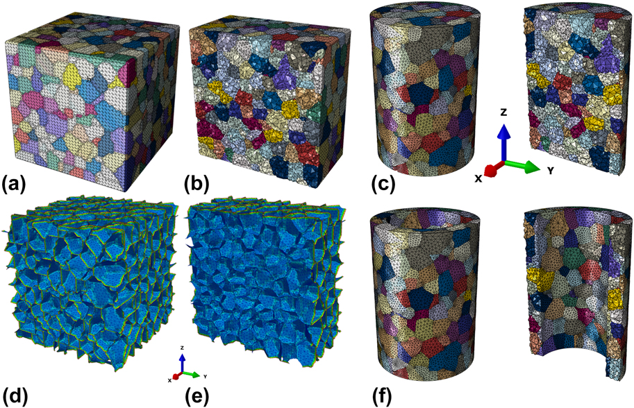
The output from DREAM.3D can be used directly in the voxel-based CP-FFT codes but, since meshing of grain structures is not a capability of DREAM.3D software, additional processing is needed to use the output to create a 3D mesh for grains and grain boundaries to be used in CPFE. In recent work by Knezevic et al.,Reference Ardeljan, Knezevic, Nizolek, Beyerlein, Mara and Pollock41,Reference Knezevic, Drach, Ardeljan and Beyerlein79,Reference Ardeljan and Knezevic80 an integrated toolset that takes grain boundary surface mesh from DREAM.3D and provides a volume mesh for each 3D grain and its grain boundary surfaces. The final polycrystalline aggregate is comprised of element sets representing individual grains [Fig. 3(a)] and grains with conformal grain boundaries between neighboring 3D grains [Fig. 3(b)]. The conformal conditions between constituent grains means that neighboring grains share triangular elements at grain boundaries.
An explicit grain structure model consisting of 784 equiaxed grains generated synthetically using DREAM.3D: (a) voxel-based model with highlighted edges, (b) triangular surface mesh. The triangular surface mesh in (b) describes grain boundaries. (c and d) The mid-section along half x-axis showing the internal structure. The edge length of the cube is 1000 µm, average grain size is 135 µm, and the total number of tetrahedral elements (type C3D4 or C3D10 in ABAQUS) in (c) is approximately 1,000,000. (e and f) FE explicit grain structure models of (a) a micropillar compression specimen consisting of 435 grains and 428,000 elements and (b) a microtube consisting of 366 grains and 276,000 elements. The outer and inner diameters are 700 and 500 µm, respectively, while the height is 1000 µm. The far-right images show the corresponding mid-sections along half x-axis to expose the internal structure. Reprinted with permission from Refs. Reference Ardeljan, Knezevic, Nizolek, Beyerlein, Mara and Pollock41, Reference Knezevic, Drach, Ardeljan and Beyerlein79, and Reference Barrett, Savage, Ardeljan and Knezevic81.

With the above technique, a 3D grain structure model in the shape of a cuboid is formed. However, sample geometries commonly encountered in testing take on other shapes, such as cylinders or tubes. Later, an advanced procedure for subtracting geometry from the cuboidal grain structure for modeling more complex shapes was developed.Reference Barrett, Savage, Ardeljan and Knezevic81 Figure 3(c) shows two examples using this model: one of a micropillar for compression and another of a microtube for microforming.
F. Kinetics of the slip and twinning mechanism in CP models
Predicting slip activity is fundamental to predicting the evolution of microstructure, textures (the reorientations of the crystals), and material flow stress with strain. Through Eq. (1.2), the theory of CP can relate slip activity on crystallographic slip and twinning systems to the distortion of a crystal. It does not, however, include criteria for the threshold of slip. Nearly all CP-based constitutive models, including the three methods presented above, mean-field, CPFE, and CP-FFT, require choosing a criterion or criteria for activating a slip system to predict slip activity.
According to the thermodynamic theory of slip, in the regime of strain rates, roughly from 10−5/s to 105/s, dislocation motion is thermally activated and dislocations must overcome energetic barriers to move. For this regime, the commonly used flow rule of viscoplasticity relating slip rate to resolved stress has a power-law form:
 $${\dot{\gamma }^s} = {\dot{\gamma }_0}{\left( {{{\left| {{\tau ^s}} \right|} \over {\tau _{\rm{c}}^s}}} \right)^{{1 \over m}}}{\rm{sign}}\left( {{\tau ^s}} \right),\;{\dot{\gamma }^s} = \left\{ {\matrix{ {{{\dot{\gamma }}_0}{{\left( {{{\left| {{\tau ^s}} \right|} \over {\tau _{\rm{c}}^s}}} \right)}^{{1 \over m}}}{\rm{sign}}\left( {{\tau ^s}} \right)} & {{\rm{if}}\;{\tau ^s} > 0} \cr 0 & {{\rm{if}}\;{\tau ^s} \lt 0} \cr} } \right.\quad ,$$
where  ${\dot{\gamma }^s}$ is the shear strain rate for a slip system s. The resolved shear stress is given by
 ${\tau ^s} = \sigma \cdot {\bf{m}}_0^s$, which is the tensor product of the stress σ and Schmid tensor
 ${\bf{m}}_0^s$, and
 ${\dot{\gamma }_0}$ is a reference slip rate (taken here as 0.001 s−1). In the exponent, m denotes the strain rate sensitivity factor. This power-law form is desirable because it provides uniqueness of solution for the active slip systems that accommodate an imposed strain rate.
The flow rule introduces a threshold value  $\tau _{\rm{c}}^s$ to activate slip. It is commonly called the the critical resolved shear stress (CRSS). Nearly all CRSS models introduced over the past several decades are phenomenological. The simplest model for the CRSS is a constant value, which does not evolve with strain. However, for calculations of deformation behavior beyond the elastic–plastic yield transition, it is desirable that the CRSS represent the resistance to move dislocations, and this value can evolve consistent with changes in subcrystalline and granular microstructure.
Many CRSS hardening models have been developed for coarse-grained polycrystals, where in the large grains, dislocations tend to accumulate in amounts that increase with strain and depend on strain rate and temperature. These stored dislocations can hinder the motion of other dislocations. This concept is used to build models for the CRSS values  $\tau _{\rm{c}}^s$ that vary as a function of strain rate and temperature.
To reflect the changes in CRSS with increasing dislocation storage, many earlier studies have adopted an extended Voce hardening law.Reference Tomé, Canova, Kocks, Christodoulou and Jonas82 This law evolves the threshold stress for each slip system in each grain with accumulated shear strain Γ according to
 $${\hat{\tau }^s} = \tau _0^s + \left( {\tau _1^s + \theta _1^s\Gamma } \right)\left( {1 - \exp \left( { - {{\Gamma \theta _0^s} \over {\tau _1^s}}} \right)} \right)\quad ,$$
where  $\Gamma = \sum\limits_s {\Delta {\gamma ^s}}$ is the accumulated shear in the grain. The Voce parameters τ0, θ0, θ1, and (τ0 + τ1) are the initial threshold stress, the initial hardening rate, the asymptotic hardening rate, and the back-extrapolated CRSS, respectively. In addition, the possibility of ‘self’ and ‘latent’ hardening are included by defining coupling coefficients h ss′, which empirically accounts for resistance against shear activity by system s associated with shear activity on system s′. The increase in the threshold stress of a system due to shear activity Δγs′ in the grain systems is then calculated as follows:
 $$\Delta {\tau ^s} = {{{\rm{d}}{{\hat{\tau }}^s}} \over {{\rm{d}}\Gamma }}\sum\limits_{s'} {{h^{ss'}}\Delta {\gamma ^{s'}}} \quad .$$
In the Voce law, temperature and rate effects are implicit in the choice of the parameters τ0, θ0, θ1, and (τ0 + τ1).
To explicitly incorporate effects of temperature and strain rate, dislocation-density (DD) based CRSS hardening models can be implemented in the place of empirical forms such as the Voce law.Reference Beyerlein and Tomé83 In DD models, the threshold stresses for slip are partly based on dislocation storage on each slip system, which evolve according to thermally activated rate laws. A general form follows, wherein the CRSS for slip on a particular slip system α is the sum of many terms: a friction stress  $\tau _{0,{\rm{f}}}^\alpha$, a forest dislocation interaction stress
 $\tau _{{\rm{for}}}^\alpha$, and a dislocation substructure interaction stress
 $\tau _{{\rm{sub}}}^\alpha$:
 $$\tau _{\rm{c}}^\alpha = \tau _{0,{\rm{f}}}^\alpha + \tau _{{\rm{for}}}^\alpha + \tau _{{\rm{sub}}}^\alpha \quad .$$
where  $\tau _{{\rm{for}}}^\alpha$ and
 $\tau _{{\rm{sub}}}^\alpha$ are resistances related to the forest DD
 $\rho _{{\rm{for}}}^\alpha$ and substructure DD
 $\rho _{{\rm{sub}}}^\alpha$, respectively. The relationship is given by the extended Taylor law as follows:
 $$\tau _{{\rm{for}}}^\alpha = \chi {b^\alpha }{\mu ^\alpha }\sqrt {\rho _{{\rm{for}}}^\alpha } \quad ,$$
 $$\tau _{{\rm{sub}}}^\alpha = {k_{{\rm{sub}}}}{\mu ^\alpha }{b^\alpha }\sqrt {{\rho _{{\rm{sub}}}}} \log \left( {{1 \over {{b^\alpha }\sqrt {{\rho _{{\rm{sub}}}}} }}} \right)\quad .$$
Here χ is a dislocation interaction parameter set to 0.9 and k sub = 0.086.Reference Capolungo, Beyerlein and Tomé84
The value of stored forest density  $\rho _{{\rm{for}}}^\alpha$ changes according to a competition between the rate of storage/generation and the rate of dynamic recovery/removal:
 $${{\partial \rho _{{\rm{for}}}^\alpha } \over {\partial {\gamma ^\alpha }}} = {{\partial \rho _{{\rm{gen,for}}}^\alpha } \over {\partial {\gamma ^\alpha }}} - {{\partial \rho _{{\rm{rem,for}}}^\alpha } \over {\partial {\gamma ^\alpha }}} = k_1^\alpha \sqrt {\rho _{{\rm{for}}}^\alpha } - k_2^\alpha \left( {\dot{\varepsilon },T} \right)\rho _{{\rm{for}}}^\alpha \quad ,$$
 $$\Delta \rho _{{\rm{for}}}^\alpha = {{\partial \rho _{{\rm{for}}}^\alpha } \over {\partial {\gamma ^\alpha }}}\left| {\Delta {\gamma ^\alpha }} \right|\quad .$$
In Eq. (1.53),  $k_1^\alpha$ is a coefficient for the rate of dislocation storage due to statistical trapping of gliding dislocations and
 $k_2^\alpha$ is the coefficient for the rate of dynamic recovery by thermally activated mechanisms (e.g., cross slip, climb). The second coefficient can be determined by
 $${{k_2^\alpha \left( {\dot{\varepsilon },T} \right)} \over {k_1^\alpha }} = {{\chi {b^\alpha }} \over {{g^\alpha }}}\left( {1 - {{kT} \over {{D^\alpha }{b^3}}}\ln \left( {{{\dot{\varepsilon }} \over {{{\dot{\varepsilon }}_0}}}} \right)} \right)\quad ,$$
where k,  ${\dot{\varepsilon }_0}$, g α, and D α are, respectively, the Boltzmann constant, a reference strain rate (taken here to be 107 s−1), an effective activation enthalpy, and a drag stress. Last, the increment in substructure density can be related to the rate of dynamic recovery of all active dislocations as
 $$\Delta {\rho _{{\rm{sub}}}} = \sum\limits_\alpha {q{b^\alpha }} {{\partial \rho _{{\rm{rem,for}}}^\alpha } \over {\partial {\gamma ^\alpha }}}\left| {\Delta {\gamma ^\alpha }} \right|\quad ,$$
where q is a rate parameter that determines the fraction of an α-type dislocations that do not annihilate, but become part of the substructure DD.
The resistance for twin activation evolves considering a temperature-independent friction term  $\tau _0^\beta$ and a latent hardening term that couples hardening between the active and inactive slip and twin systems. Accounting for both effects, the resistance for twinning is expressed as
 $$\tau _{\rm{c}}^\beta = \tau _0^\beta + {\mu ^\beta }\sum\limits_\alpha {{C^{\alpha \beta }}{b^\beta }{b^\alpha }\rho _{{\rm{for}}}^\alpha } \quad .$$
In this relationship, μβ, b β, and C αβ represent, respectively, the elastic shear modulus, Burgers vector on the given twin system, and the latent hardening matrix used for coupling.
Last, these laws have considered the effects of the microstructure, most often grain size D, according to a Hall–Petch law. The Hall–Petch-like term follows the equationReference Beyerlein and Tomé83
 $$\tau _{0,{\rm{HP}}}^\alpha = {{{H^\alpha }{\mu ^\alpha }\sqrt {{b^\alpha }} } \over {\sqrt {d_{{\rm{mfp}}}^\alpha } }}\quad ,$$
where, H α, b α,  $d_{{\rm{mfp}}}^s$, and μα are the Hall–Petch coefficient per slip mode, the mean free path is defined as the distance along the slip plane of slip system α from one boundary to the next. Thus, h α′ depends on the orientation of the crystal with respect to the interface normal and the layer thickness h.
G. Advantages and disadvantages of mesoscale methodologies
Having reviewed the elements involved in these mesoscale methodologies, it is worth remarking on their advantages and disadvantages when it comes to modeling PMP relationships.
One of the first and to this day commonly used CP polycrystal models is the full constraint Taylor model. It solves for the stress in each grain assuming that the strain and strain rate in each grain equals the macroscopic strain and strain rate. The two mean-field codes we reviewed, VPSC and EPSC, are effective tools for estimating the uniform grain stress and strain (and strain rate) in each grain within a polycrystal.Reference Lebensohn, Castañeda, Brenner, Castelnau, Ghosh and Dimiduk85 Unlike the Taylor model, the grain stress, strain rate, and shape in the self-consistent formulations will deviate from the average or macroscale stress, strain rate, and applied deformation, respectively. Bulk texture and grain shape distributions are predicted well, comparable to the full field, spatially resolved techniques. They are computationally efficient and can be executed with minimal computational cost on a standard desktop (laptop) computer. They are ideal for multiple simulations for different loading conditions, involving changes in strain path, rates, and temperatures, and for the large strain deformation characteristic of metal forming processes.
In VPSC and EPSC, iterations are required at both the single crystal level and the self-consistent level. In practice, the number of iterations is subject to a prescribed value of tolerance and the chosen convergence criterion. Usually, 10 iterations are needed at the single crystal level and 4–6 iterations at the polycrystal level. The first time increment and the increments at the elastoplastic transition in EPSC typically require more iterations than these common values. Furthermore, these numbers vary with crystal orientations and imposed deformation state. For the same problem, the self-consistent schemes can be up to one order of magnitude slower than the full constraint Taylor model for the same time increment. In the authors’ experience, 4–6 self-consistent iterations are typically observed, and as a result, self-consistent models are 4–6 times slower than Taylor-type models.
Compared to mean-field approaches, CPFE and FFT can yield additional information on the effects of grain–grain interactions, intragranular stress and strain evolution, and heterogeneous onset of localization, all of which are important for understanding and designing metal processes, as will be demonstrated shortly. They also account for local neighborhoods and spatial resolution in the mechanical fields below the grain scale, such as stress concentrations at boundaries and intersections of many boundaries (e.g., triple points, twin/grain boundary intersections). These capabilities are important for modeling many boundary driven mechanisms that are sensitive to a combination of interface morphology, character, and crystal orientation, as will be shown later as well. However these capabilities make them more computationally expensive and reliant on realistic representations of 3D microstructures (as described earlier in Sec. II.E).
III. MESOSCALE INSIGHTS INTO PMP RELATIONSHIPS
Processing alters many mesoscale aspects of the material microstructure, and among them, the main mesoscale microstructural features are texture, grain size, twin volume fraction, and dislocation density. These microstructural features impact the deformation response, including yield strength and ultimate strength, and perhaps more importantly, the anisotropy in strength. Advantageously, the standard versions of the aforementioned models can relate processing to evolution in these important mesoscale quantities as well as the microstructure after processing to the deformation response measured in mechanical testing.
Many high performance materials are inherently or microstructurally complex, warranting advancements in these methods beyond the standard versions. While the basic rigorous mechanics formulations are preserved, the extensions and their applications have varied in recent years, and therefore, a good representation of the state-of-the-art in mesoscale modeling requires presenting many examples.
The examples in this section cover studies that have used and extended mesoscale 3D, full field spatial resolved computational models to investigate processing–microstructure relationships in polycrystalline materials. These include examining the influence of strain and stress fluctuations at grain boundaries on the onset of deformation twinning or on shear banding. The need for discrete modeling in this area arose since no theory or continuum counterpart could address the problem.
A. Implementing grain boundary stress fluctuations and role in the evolution of deformation twinning into mesoscale polycrystal models
Over the years, a series of studies have been performed to develop a multiscale polycrystal model for metals with low-symmetry crystal structures that deform easily by slip and twinning. Many of these models couple a SC scheme, either VPSC or EPSC, with a twin reorientation scheme, such as PTR or CG, as described in Sec. II.B. As mentioned, the model produces calculations of grain average stresses as a function of its orientation and shape. These conventional polycrystal SC-TW models can use these grain-level stresses to determine if the grain will form a twin. The threshold to activate twinning is usually a constant value, assigned a priori.
Mesoscale models are still faced with the problem of how to capture twinning and its evolution in a polycrystalline microstructure for two reasons. First, twin initiation occurs in the vicinity of internal boundaries and at certain exceptional points in the boundaries. In a deforming polycrystal, apart from large defects such as cracks, experimental observations suggest that grain boundaries are the most likely areas for twin formation.Reference Beyerlein, Zhang and Misra23,Reference Arul Kumar, Beyerlein, McCabe and Tomé24,Reference Beyerlein, Capolungo, Marshall, McCabe and Tomé86–Reference Meyers, Andrade and Chokshi88 Second, it is well known that twin nucleation is a statistically rare event, for which activation is largely controlled by a combination of probabilistic events. In the case of formation of twins from grain boundaries, twinning depends sensitively on the likelihood of having the right local atomistic configurations combined with highly localized stress concentrations. Thus, the mesoscale challenge is predicting the evolution of twins, occurring stochastically in time and spatially when the governing factors involve local aspects of internal boundaries.
In a few recent studies,Reference Niezgoda, Kanjarla, Beyerlein and Tomé36,Reference Beyerlein and Tomé89 a probabilistic approach was developed to include grain-boundary-induced twin nucleation into mean-field CP models, like VPSC with a twin reorientation scheme. Unlike conventional polycrystal models to date, the model they used for twin nucleation is not deterministic but dictated by twin formation from points in grain boundaries, where high stresses and weak defect sources simultaneously happen.
The approach involved incorporating two aspects of the grain boundaries in a bulk average probabilistic sense. One aspect was a probability model for the nucleation of twins when some numbers of grain boundary defects undergo stress-driven transformations, forming several small nuclei which then coalesce into a single stable nucleus.Reference Beyerlein and Tomé89 It assumes that the timescale of the transformation and subsequent coalescence is instantaneous compared to the applied deformation and introduces a characteristic length scale, within which a critical number of transformations occur to produce a propagating twin. The stochastic model gives an explicit form for the probability distribution for the critical stress values required for twin nucleation that could be used in the VPSC model for activating twinning.
The other issue concerned the stresses that activate twinning. These stresses are those that are generated at grain boundaries and these tend to deviate significantly from the average stresses calculated in VPSC for each grain. To tackle this, distributions of grain boundary stresses were obtained from separate full-field CP calculations. Taken together, the VPSC model simulations of deformation were advanced to activate twinning when a randomly sampled critical twin stress was exceeded by a randomly sampled grain boundary stress.
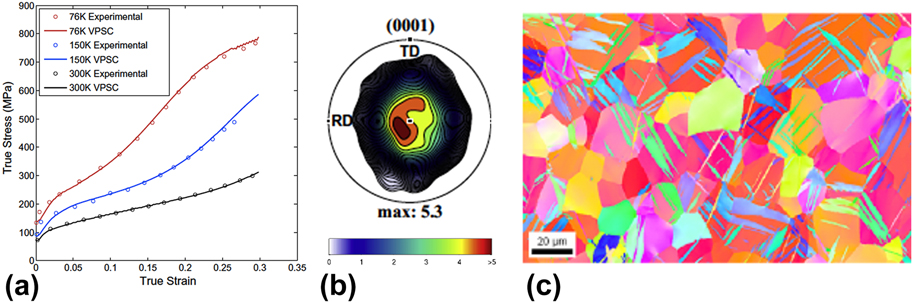
As an example, Figs. 4(a) and 4(b) show the initial texture and flow response of the polycrystalline Zr sheet material when tested in simple compression at three different temperatures: 76, 150, and 300 K. The initial texture is a strong basal texture resulting from the clock rolling procedure.Reference Beyerlein and Tomé83 As can be seen in Fig. 4(b), most of the c-axes of the hexagonal close packed (HCP) crystals of Zr are highly aligned in the through-thickness direction of the sheet. The loading direction in the tests shown in Fig. 4 is intentionally perpendicular to the plate normal so that deformation twinning would be favored, see Fig. 4(c). The drastic differences in the shapes of the curves, yield stress, and hardening behavior are a consequence of the underlying interplay of slip and the formation and propagation of deformation twins.
Deformation of rolled high purity Zr: (a) comparison of the experimental and calculated stress–strain curves at three different temperatures, 76 K (red), 150 K (blue), and 300 K (black). (b) The basal pole figure of the initial texture and (c) EBSD image of the Zr after 10% deformation showing the extension twins. Reprinted with permission from Ref. Reference Niezgoda, Kanjarla, Beyerlein and Tomé36.

Unlike slip, deformation twinning accommodates deformation in one sense of the direction but not the other, and therefore twinning is one source of plastic anisotropy, particularly in highly textured materials, with low-symmetry crystal structure (such as Mg, Ti, Be, and their alloys). The mechanisms that are responsible for the onset of twinning, and its propagation, are currently subjects of intense study. Numerous experimental studies find that in most cases, twinning is more likely to occur as the grain size increases and in suitably oriented grains, where the resolved stresses on the twin plane and twin direction are high.Reference Beyerlein, Zhang and Misra23,Reference Beyerlein, McCabe and Tomé35,Reference Meyers, Andrade and Chokshi88,Reference Beyerlein, McCabe and Tome90,Reference Lentz, Risse, Schaefer, Reimers and Beyerlein91
As mentioned, 3D full field CP-FFT simulations were used to calculate the stress fluctuations that would develop in the grain boundaries in the initial loading stages during the compression of the Zr sample. The FFT-based algorithm computes a compatible strain-rate field that minimizes the average work rate under the constraints of the constitutive relation and stress equilibrium. Consequently, variation in grain boundary character will introduce a randomness into the stress field.
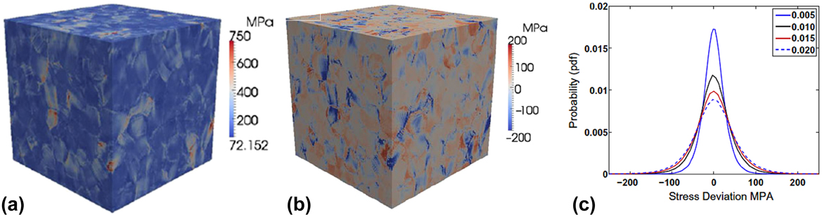
For this particular calculation, the 3D RVEs were created using the DREAM.3D digital microstructure analysis environment. Figure 5(a) shows simulations for one representative volume, comprised of approximately 500 grains with an initial rolling (basal) texture, similar to the one in the material tested experimentally in Fig. 5(b). The inhomogeneous stress distribution is shown in Fig. 5(a), and the stress fluctuations as a selected strain level are shown in Fig. 5(b). The latter was obtained by calculating the grain average stresses and subtracting it from the total stress. We observe significant deviation from the average grain stress at the grain boundaries and that the highest stress deviations occur at the boundaries. Many grains have both compressive (“cold”) and tensile (“hot”) deviations from the grain average. Figure 5(b) shows the locations of hot spots in red and cold spots in blue. Interestingly, hot and cold spots corresponded to regions where three or more grains meet and not within the interiors of grains. A similar outcome was reported previously in a study of deformed FCC polycrystals, using another 3D full-field CP model based on a Green’s function homogenization scheme.Reference Rollett, Lebensohn, Groeber, Choi, Li and Rohrer92 For twin nucleation, the interest lies in the “hot spots”.
CP-FFT calculation of polycrystalline Zr in deformation showing the (a) von Mises stress and (b) stress fluctuations for 550 grains. (c) Distribution of the stress fluctuations after different strain levels ranging from 0.5% strain to 2% strain. Reprinted with permission from Ref. Reference Niezgoda, Kanjarla, Beyerlein and Tomé36.

For use in VPSC simulations, the CP-FFT calculations were repeated for an ensemble of 100 representative Zr material volumes to produce a statistically significant probability distribution for the components of the stress fluctuations generated at the grain boundaries in a deforming polycrystal. The stress fluctuation tensor is made up of six components, and all six are subjected to the VPSC simulations. Figure 5(c) shows the observed deviation of the σ11 component from the grain stress,  $\sigma _{11}^{{\rm{fluc}}}$ at selected strain levels. Due to the averaging over multiple loading conditions, the fluctuations on all three normal components had approximately the same near-Gaussian distribution, as did the three shear stress components. The extreme tails of the distributions extend significantly farther than would be expected from a perfect Gaussian.
The VPSC model incorporating the stochastic approach to twinning was used to calculate the deformation of Zr and the underlying twinning microstructure (distribution of twin variants, twinned grains, and twin thickness). Figure 4(a), shown earlier, also compares the VPSC calculated stress–strain curves at 76 K, 150 K, and room temperature (300 K) with the experimental curves. Incorporation of the new twin nucleation model leads to flow stresses and hardening rates in excellent agreement with measurement across the full temperature spectrum, an achievment not possible with the conventional (deterministic approach) to twin activation.
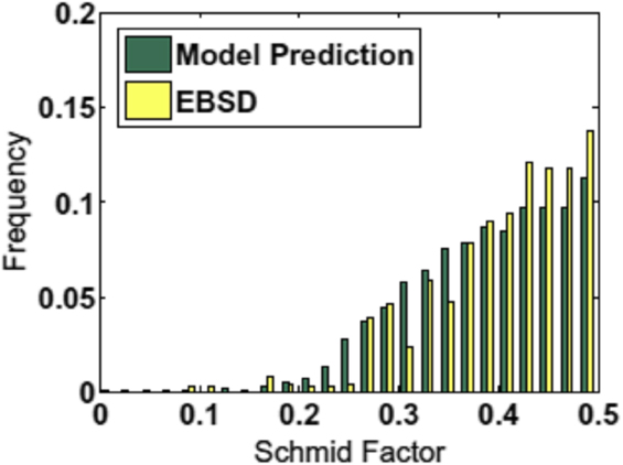
Calculations of the twinning microstructure are compared with reported statistical electron backscatter diffraction (EBSD) characterization in the same deformed zirconium at multiple temperatures. One signature that indicates that twinning is not deterministic is the report of “non-Schmid twins”. Twins that form in grains are expected to be the variant that has the highest Schmid factor (among the six possible) and surprisingly many of the twins formed in deformed materials are twin variants of lesser rank, or not those with the highest Schmid factor. Figure 6 compares the calculated and measured number distribution after 10% strain and at 76 K. Both the model and measurement are in agreement in several factors. The frequency of twins with a given Schmid factor m increases with m, which means that most of the twins (and most of the twin volume fraction) are concentrated in grains that are well oriented for twinning (i.e., those with high Schmid factors). Also, the distributions are broad, with the frequency of twins with low Schmid factors being non-negligible. Thus, a significant fraction of twins have formed in grains less favorably oriented. The analysis confirms that the observation of non-Schmid twins arises because twin variant selection is a stochastic process.
Comparison of the Schmid factors for the twins that have formed in Zr after 10% strain according to the measured (EBSD) and calculations. Reprinted with permission from Ref. Reference Capolungo, Marshall, McCabe, Beyerlein and Tomé87.

The VPSC model with the stochastic twinning approach demonstrates a viable method for introducing local, lower length scale, boundary-driven deformation in mesoscale modeling. Specifically, this combined, serial application of CP-FFT and VPSC work showcases inclusion of multiscale effects via the introduction of stochasticity. The general idea is that the lower length scale features are not explicitly captured in higher length scale models. Rather, the distribution of possible states at the lower length scale associated with a state at the higher length scale is introduced through a probability model. In doing so, important effects that the shorter length scales can exert on the higher length scales can be taken into account without the need to explicitly carry the lower scale structural details through the simulation.
B. A combined full-field/mean-field model for texture gradients and twinning during the rolling of low-symmetry materials
Most often, the rolling process is modeled as plane strain compression, which represents best the deformation of the center of a rolled sheet. In the actual rolling process, the deformation state at the sheet surfaces where the material meets the rolls can differ from the center. Such gradients in deformation have been shown to result in gradients in texture and other microstructural aspects, usually for cubic materials, such as Cu and Al and steel.Reference Kocks, Tomé and Wenk93 However, their severity and extent will be more pronounced the greater the inherent elastic and plastic anisotropy of the material. For highly elastically and plastically anisotropic materials (such as hcp Ti, Mg, and Zr, and orthorhombic uranium, U), calculation of deformation-induced texture gradients would be better predicted with a mesoscale technique that strongly couples the evolution of texture, local anisotropic crystalline response, and nonuniform boundary conditions.
Recent work used a multiscale FE-VPSC model to simulate the development of texture in α-uranium.Reference Zecevic, Knezevic, Beyerlein and McCabe94,Reference Knezevic, Crapps, Beyerlein, Coughlin, Clarke and McCabe95 Uranium is a prime example of a metal that is highly anisotropic. Pure U at ambient pressures and temperatures (up to 623 K) has an orthorhombic crystal structure.Reference Yoo96,Reference Daniel, Lesage and Lacombe97 It deforms by multiple slip and twinning modes differing in their activation stresses, and, like most metals possessing a low-symmetry crystal structure, plastic deformation is highly anisotropic and sensitive to texture.
The preferred slip and twinning modes for U have been identified previously.Reference Lebensohn and Tomé5,Reference Daniel, Lesage and Lacombe97–Reference Choi and Staker105 The easiest slip mode is (010)[100], possessing only one slip system. Another easy slip mode is called floor slip (001)[100], again possessing one slip system, which serves as a secondary slip mode, enabled by cross slip from (010)[100] up to 623 K but becomes the primary slip mode above 623 K. The next easiest slip mode is the 1/2 {110} $\left\langle {1\bar{1}0} \right\rangle$ slip mode, which has two slip systems. The chimney 1/2
 $\left\{ {1\bar{1}2} \right\}$〈021〉 slip mode is more difficult but is necessary to accommodate plastic strain in the [001] direction. The observed twinning modes are {130}
 $\left\langle {3\bar{1}0} \right\rangle$, and {172}
 $\left\langle {3\bar{1}2} \right\rangle$ and its reciprocal twin {112}
 $\left\langle {3\bar{7}2} \right\rangle$. The former is considered the easiest one. The twin shear S of the {130}
 $\left\langle {3\bar{1}0} \right\rangle$ twin is 0.299 and it reorients the lattice by 69.3° about [001]. For the {172}
 $\left\langle {3\bar{1}2} \right\rangle$ twin, S = 0.227, and it reorients the lattice by 92.6° about
 $\left\langle {\left( {10} \right)\bar{7}0} \right\rangle$.
In their approach, FE and VPSC are combined concurrently, wherein the deformation of the sample as it is rolled is calculated using FE and the constitutive response at each integration point is supplied by VPSC. The kinetics of slip are modeled using a rate-sensitive flow rule and lattice reorientation due to deformation twinning by the CG model (see Sec. II.B.3). At the subgrain scale, the threshold stresses for activating slip are governed by the evolution of stored dislocation density on the slip system according to thermally activated rate laws and hence are explicit functions of temperature and strain rate (see Sec. II.F).
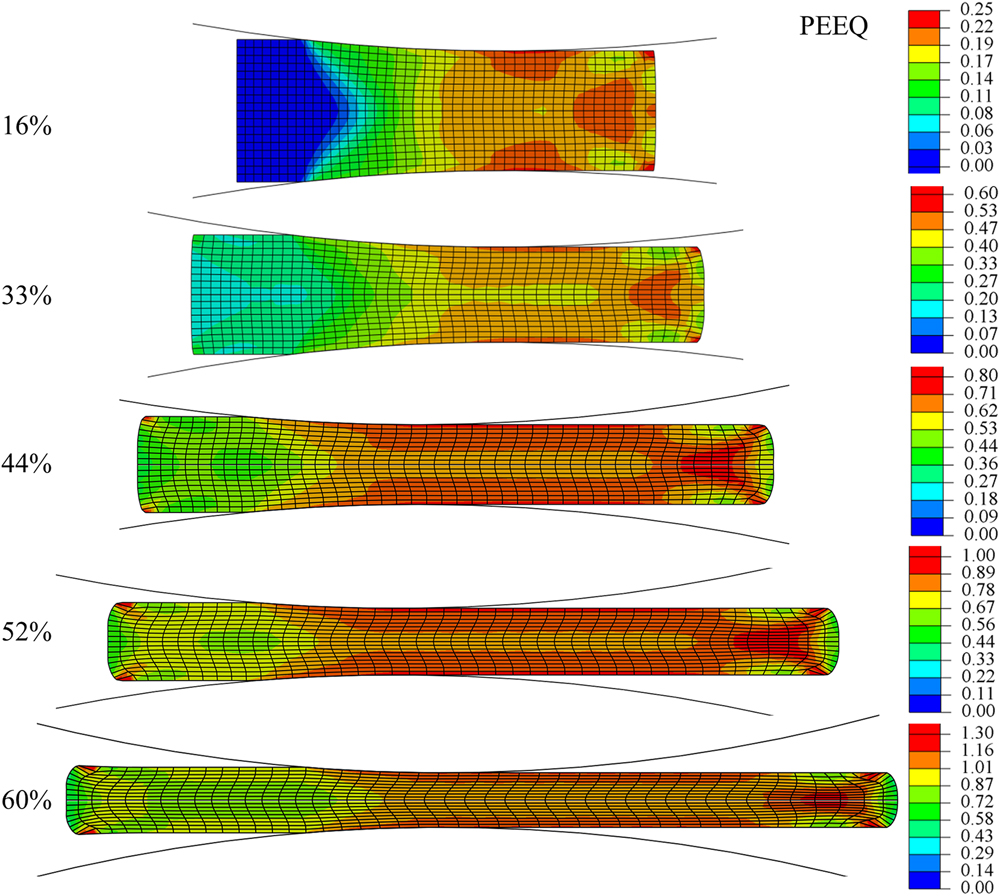
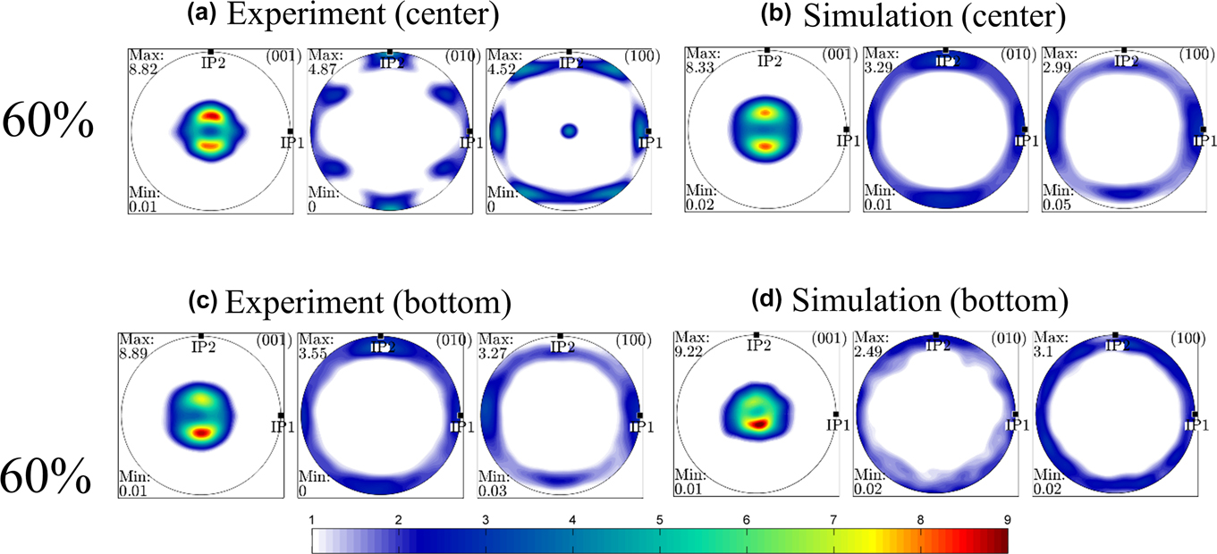
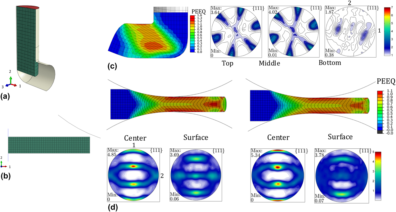
Figure 7 shows calculated equivalent plastic strain contours after each rolling pass for five rolling passes. As shown, the FE simulation forecasts that strains develop nonuniformly in the sheet, varying both from end to end and through the thickness of the sheet. The impact on texture development through the thickness of the sheet can be seen in Fig. 8. These textures from both the measurement and the model are presented using pole figures for the top and bottom surfaces and the center. Overall, the texture is very strong; two pronounced maxima are observed in the {001} pole figures, both in the experiment and model prediction, at all points through the thickness.
Fields of PEEQ after each subsequent rolling pass of pure alpha uranium. Reprinted with permission from Ref. Reference Zecevic, Knezevic, Beyerlein and McCabe94.

Pole figures comparing the (a and c) measured and (b and d) calculated texture in pure uranium after 60% accumulated strain at a point in (a and b) center and (c and d) near the surface of the sheet. Texture was measured and taken from simulations approximately 10 mm from the exit. Reprinted with permission from Ref. Reference Zecevic, Knezevic, Beyerlein and McCabe94.

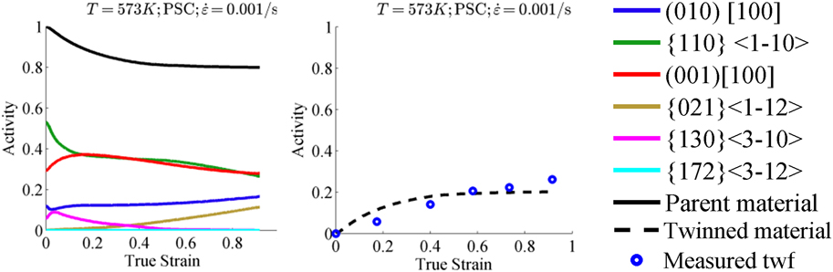
One valuable output from CP models is slip activity within the grains, which is hard to assess experimentally (Fig. 9). The predominant slip modes operative during rolling are floor slip (001)[100], and chimney slip 1/2 {110} $\left\langle {1\bar{1}0} \right\rangle$. Twinning via the {130}
 $\left\langle {3\bar{1}0} \right\rangle$ mode is activated in rolling and, in agreement with experiments, achieves a significant twin volume fraction (calculated to be 25% by the end of the rollig pass). Within the twin domains, the model predicts that chimney and floor slip modes are active. The model finds that the grain orientations associated with the two distinct maxima on the (001) pole figure deformed predominantly by floor (001)[100] slip and are strengthen by
 $\left\{ {130} \right\}\left\langle {3\bar{1}0} \right\rangle$ twins.
Relative activities of deformation modes and a comparison between measured and predicted twin volume fraction during plane strain compression of α-U at 573 K. Reprinted with permission from Ref. Reference Zecevic, Knezevic, Beyerlein and McCabe94.

In the model, the surface textures are observed to develop differently than those in the center. Comparisons with prior calculations with stand-alone VPSC shows that the center texture is similar to that predicted from the ideal plane strain compression assumption, whereas the surface textures are not. For validation, particular points through the thickness of the sheet are compared with EBSD measurements, as described in Sec. II.B.3, Fig. 1. The notable difference in the surface and center textures is an asymmetry in the two predominant peaks in the {001} pole figure. Moreover, the bottom and top surface textures are different. While the texture component with the peak intensity in the bottom texture lies in the lower maxima, the peak in the texture at the top surface lies at the upper maxima. The difference is a result of the shear stress state imposed by the rolls at the surface.
The ability of this mesoscale numerical tool to predict these gradients, in spite of the computational expense, can lead to better understanding and predictions of recrystallization kinetics and finally recrystallized microstructures (grain size, texture) during post-rolling heat treatments. Gradients in texture will influence many microstructural features believed to affect recrystallization, such as crystallographic orientation, gradients in orientation, gradients in stored energy in the grains, and near the grain boundaries, and the distributions in the properties of grain boundaries.
C. A 3D full-field, spatially resolved CP model for shear banding during the rolling of two-phase laminates
An important issue encountered in fabricating two-phase system laminate structures via metal forming techniques, such as rolling, is plastic instabilities. The onset of instabilities, such as (noncrystallographic) shear bands that cut across many grains, during the rolling process can prevent continuity in layers and detrimentally affect subsequent properties, as will be shown later.Reference Ardeljan, Knezevic, Nizolek, Beyerlein, Mara and Pollock41,Reference Wu, Chang, Maawad, Gan, Brokmeier and Zheng106,Reference Yang, Cizek, Hodgson and Wen107 For processing, it is best to use a model to guide on where and when such instabilities are likely. Very recently, CPFE has been applied to simulate the rolling of two-phase lamellar FCC/FCC and FCC/BCC compositesReference Bronkhorst, Mayeur, Beyerlein, Mourad, Hansen, Mara, Carpenter, McCabe and Sintay108–Reference Jia, Eisenlohr, Roters, Raabe and Zhao113 and HCP/BCC composites.Reference Ardeljan, Knezevic, Nizolek, Beyerlein, Mara and Pollock41 In the rolling simulations, localized areas of stress or strain concentrations developed, which could provide a source for shear banding. Simulating the transition from such localized stress or strain to shear banding, however, requires incorporating an additional, noncrystallographic shear band systemReference Jia, Eisenlohr, Roters, Raabe and Zhao113 or a local softening criterionReference Ardeljan, Knezevic, Nizolek, Beyerlein, Mara and Pollock41 into the CPFE model.
Recently, Ardeljan et al.Reference Ardeljan, Knezevic, Nizolek, Beyerlein, Mara and Pollock41 developed a 3D microstructure-based, full-field CPFE to study the onset of shear banding during the rolling of a two-phase HCP-Zr body centered cubic (BCC) Nb composite. For both the Zr and Nb phases, the constitutive model used anisotropic elasticity and a thermally activated DD-based model for activating slip. Figure 10(a) shows the starting microstructure. This microstructure models was created using a synthetic grain structure builder (DREAM.3D) and a meshing toolset for the 3D network of grains, grain boundaries, and bimetal interfaces (see Sec. II.E). The crystal orientations, grain shapes, and grain sizes for each phase were initialized based on the measured data.
(a) Numerical setup of the 127 mm layered microstructure of the model synthetic polycrystalline aggregate with 1200 mm in RD, 480 mm in TD, and 1320 mm in ND. The FE mesh of 3D grains consisted of 1.5 million C3D4 (continuum 3D 4-node) tetrahedral elements. (b) Distributions of the normalized value of equivalent plastic strain (PEEQ) at true strains of 0.1 and 0.2 showing strain heterogeneities developing at grain boundaries and triple/quadruple junctions. Red circles indicate hot spots forming a band. Black circles indicate hot spots disappearing and not forming a band. Blue circles indicate cold spots. (c) Shear banding after softening elements experiencing hot spots: deformed grain structure (top) and distributions of equivalent strain normalized by the applied equivalent plastic strain (bottom) after subsequent straining of 0.2. Reprinted with permission from Ref. Reference Ardeljan, Knezevic, Nizolek, Beyerlein, Mara and Pollock41.

Using this multiscale model, simulations of plane strain compression are carried out to investigate the connection between microstructural evolution and the onset of strain localizations in 3D. Figure 10(b) shows a typical slice of the 3D microstructure after a relatively moderate amount of strain (10%). Hot spots were assigned regions with strain concentrations greater than 1.5 and cold spots regions with concentrations lower than 0.5. Analysis of the entire polycrystals reveals that local areas of relatively high (and relatively very low) strain concentration occur at triple junctions or quadruple points, as in the prior CP-FFT studies for FCC and HCP polycrystals. It was found that the hot spots connect via straining to create a banded configuration that extends across many grains in the polycrystalline layer. This event starts in the Zr phase and not in the Nb phase, and the triggering hot spots in strain occur at junctions that join grains with very dissimilar reorientation propensities and vice versa for cold spots. When an additional softening mechanism (by lowering the dislocation density at this points) is introduced into the model, these localized strain concentration areas in the Zr phase can lead to shear bands, as shown in Figs. 11(c) and 11(d).
Optical micrographs showing lamellar microstructures in the Zr/Nb composite produced by the ARB process with an annealing step after every other ARB pass. For (a–c), strain levels/number of layers/average layer thicknesses in mm are as follows: 2.7/16/127, 3.5/32/58, and 4.1/64/30. The micrographs at 127 and at 30 mm layer thicknesses are shown after the annealing step. (d) 4 µm layer thickness micrograph before annealing showing the shear bands. (e) TEM micrograph of nanolayered Zr/Nb with an average layer thickness of 88 nm. Reprinted with permission from Refs. Reference Carpenter, Nizolek, McCabe, Knezevic, Zheng, Eftink, Scott, Vogel, Pollock, Mara and Beyerlein115 and Reference Carpenter, Nizolek, McCabe, Zheng, Scott, Vogel, Mara, Pollock and Beyerlein114 (Ref. Reference Carpenter, Nizolek, McCabe, Zheng, Scott, Vogel, Mara, Pollock and Beyerlein114 covered Creative Commons license CC BY 3.0—http://creativecommons.org/licenses/by/3.0).

Often, intermediate annealing steps between rolling steps are used to soften the material. Using this multiscale model, simulations of plane strain compression are carried out to investigate the connection between the microstructural changes associated with annealing and the onset of strain localizations in 3D. Three annealing-induced changes were investigated systematically: reduction in the accumulated DD, alterations in the crystallographic texture, changes from an elongated to equiaxed grain shape. It was shown that while it is difficult to avoid strain localizations at grain junctions, when provided a microstructure containing a few large grains spanning the thickness (less junctions), elongated grain shapes (consistent with rolling deformation), and reduced DD (lower plastic anisotropy), the formation and subsequent linkage of hot spots in the form of a band can be postponed.
With insight from the model, a second attempt involving periodic annealing treatments (575 °C for one hour) between ARB rolling passes was introduced in the laboratory. These extra steps enabled refinement to the same thickness without shear band formation (Fig. 11). Due to the successful suppression of shear band formation, material with individual layer thicknesses of ∼90 nm was achieved through further processing.Reference Carpenter, Nizolek, McCabe, Zheng, Scott, Vogel, Mara, Pollock and Beyerlein114,Reference Carpenter, Nizolek, McCabe, Knezevic, Zheng, Eftink, Scott, Vogel, Pollock, Mara and Beyerlein115 The 4 µm layer thickness micrograph is provided before annealing to show the shear bands.
D. Additively manufactured materials
An exciting and swiftly emerging manufacturing process for metallic materials is additive manufacturing (AM). Over the period of its growth, the focus of AM has shifted from prototyping to manufacturing fully functional end-use parts. Direct metal laser sintering (DMLS), as an AM technology, is increasingly being evaluated to complement production of complex shaped parts in the aerospace industry. DMLS, like other AM technologies, has the advantage of eliminating the need for extensive machining and expensive tooling over traditional manufacturing techniques, such as forging. It remains to be confirmed whether the parts produced using this novel manufacturing technology perform at the same level as wrought or cast counterparts under various monotonic or cyclic loading conditions and temperatures typical for their expected applications.
In the AM process, the grain shapes can take on unusual morphologies, differing from the equiaxed or ideally layered shapes of the materials addressed thus far. Figure 12 shows EBSD maps of two different materials processed by AM, the IN718 Ni-based superalloy and MarM509 Co-based superalloy, demonstrating the elongated and rough appearance of grains that can form from this process.
EBSD maps showing the initial microstructure in the samples of AM (a) Inconel 718 and (b) MarM509. The colors in the maps indicate the orientation of the built direction (aligned with the axis of vertically built samples) with respect to the crystal reference frame according to the IPF triangle. Below the EBSD image are the pole figures showing the corresponding texture. Reprinted with permission from Ref. Reference Ghorbanpour, Zecevic, Kumar, Jahedi, Bicknell, Jorgensen, Beyerlein and Knezevic118.

The microstructure and texture produced from this process tend to depend strongly on the direction in which the sample was built (BD). The samples of IN718 were “printed” by the DMLS process in the form of bars and rods and then subsequently machined into the mechanical test samples. The heat treatment needed to produce the final superalloy structure containing a high fraction of γ′ and γ″ phases and a lower fraction of the δ phaseReference Wang and Li116,Reference Kuo, Yang, Bor, Wei and Tai117 was applied after printing and directly to the machined test samples.
The EBSD image in Fig. 12(a) of the mesoscale microstructure after all these processing steps displays many columnar grains with an average aspect ratio of 5 (major axis a = 65.93 μm and minor axis b = 13.16 μm) along the BD. The corresponding pole figures shown in Fig. 12(a) indicate that the material possessed a moderately strong 〈001〉 texture component again along the BD, with an m.r.d. of nearly 3. The directional columnar grain structure and preferred texture are a consequence of the heat flow roughly perpendicular to the surface of the substrate during AM.
The anisotropic grain morphology and texture are expected to give rise to plastic anisotropy, with properties depending on the test direction with respect to the BD. Figure 13 shows the deformation response in uniaxial tension or uniaxial compression in different directions with respect to the BD: Vertical-V (aligned with the BD), diagonal-D, and horizontal-H (normal to the BD). All curves exhibit a classical decreasing hardening rate, a signature of the slip-dominated plastic deformation. In both tension and compression, the flow stress is found to depend on the loading direction with respect to the build direction. The anisotropy was similar in both tension and compression. The strongest direction was D, the second H, and the weakest V. The difference was non-negligible, being, for instance, 7% between the D- and V-direction tensile strengths. Another important anisotropic factor to extract from these tests is tension-compression asymmetry. All build directions (V, D, and H) exhibited significant T–C asymmetry, wherein the tensile flow stresses are lower than the compression flow stresses.
Comparison of measured and predicted true stress–true strain responses in tension and compression of IN718 as a function of build direction as indicated in the figure. The compressive curves went to large strains, while the tensile curves terminated at much smaller strains (<0.2). Reprinted with permission from Ref. Reference Ghorbanpour, Zecevic, Kumar, Jahedi, Bicknell, Jorgensen, Beyerlein and Knezevic118.

Very recently the EPSC model was applied to relate the deformation response of a Ni-based superalloy with the build direction.Reference Ghorbanpour, Zecevic, Kumar, Jahedi, Bicknell, Jorgensen, Beyerlein and Knezevic118 EPSC is well suited for understanding the influence of grain shapes and texture on the elastic and plastic deformation of polycrystalline materials, even in these extreme grain morphology cases. EPSC directly accounts for the constraint effects that extreme grain shapes can impose on the deformation of grains in a polycrystal. In this case, the stress and strain rate and lattice reorientation and slip activity in every grain are direct outcomes of the direction of loading with respect to the grain axes. The standard EPSC does not, however, account for the directional hardening that odd grain shapes can impose. In the EPSC model in Ref. Reference Ghorbanpour, Zecevic, Kumar, Jahedi, Bicknell, Jorgensen, Beyerlein and Knezevic118, the directional hardening caused by the grain shape was implemented.
The added anisotropic effect posed by grain shape is a microscopic one and concerns the restriction that grain boundaries can have on the distance traveled by dislocations (the dislocation mean free path). Specifically, dislocation travel distance depends on the orientation of the slip plane of system s with the grain boundaries,  $d_{{\rm{mfp}}}^s$. For instance, when grains are equiaxed, the nearly spherical grain shape would pose no anisotropic resistriction on the dislocation mean free path and all slip systems have equal
 $d_{{\rm{mfp}}}^s$. By contrast, for grains with extreme shapes, bearing large aspect ratios, some slip systems will be oriented with shorter travel distances than others and hence will be relatively harder. The shape effects on
 $d_{{\rm{mfp}}}^s$ were represented microscopically using the Hall–Petch law in Eq. (1.57). The
 $d_{{\rm{mfp}}}^s$ for any slip system s in a grain with an instantaneous major axis a and minor axes b and c can be estimated by
 $$d_{{\rm{mfp}}}^s = {2 \over {\sqrt {{{\left( {{{\hat{b}_x^s} \over a}} \right)}^2} + {{\left( {{{\hat{b}_y^s} \over b}} \right)}^2} + {{\left( {{{\hat{b}_z^s} \over c}} \right)}^2}} }}\quad ,$$
where  $\hat{b}_x^s,\;\hat{b}_y^s,\;\hat{b}_z^s$ are the components of a unit vector in the slip direction expressed in a frame of the ellipsoid. Equation (1.58) finds the longest possible distance in the slip direction with respect to the ellipsoid. A minor effect for local crystallography enters through the use of the slip-system shear modulus projected on the slip plane and slip direction.
The EPSC model was used to simulate uniaxial tests in different build directions (vertical-V, diagonal-D, and horizontal-H) and as shown in Fig. 13, produce good agreement in yield stress, ultimate stress, and hardening with all measured responses. Since these were room temperature tests, the model presumed that the active slip mode was the common one for FCC metals: {111}〈110〉. Most importantly, the anisotropy in yield was captured, leading to a higher stress in the D sample and second in the H sample in either compression or tension, a result that can be attributed to the active slip systems in the elongated grains having a shorter mean free path in D than in V. To summarize, the model finds that the plastic anisotropy, e.g., the percentage differences and ordering, is due to the combined result of texture and grain shape, resulting from the AM process.
IV. MAKING 3D MULTISCALE PROCESSING-MICROSTRUCTURE MODELING FASTER
Thus far, this review paper has discussed the latest development in 3D, mesoscale CP-based modeling techniques and some recent advancements in the ability to model the role that mesoscale microstructural features, such as grain (orientation, size, and shape) and grain boundaries, play in the development of local stress states and deformation mechanisms during mechanical processing or straining. In many of the processing–microstructural studies reviewed here, it is clear that great computational expense is required to account for phenomena across mesoscale length scales. At present, it would be too computationally intensive to consider concurrently the macroscopic boundary conditions across a part and the evolution of texture down to the dynamics of slip at one of the interfaces. Methods for boosting computational speed are needed if the field wishes to exploit the ability of a fully 3D mesoscale model to probe a wide range of extensive and intensive variables across a broad range length and time scales. In this section, we discuss some new and upcoming strategies for improving computational speed of mesoscopic, microstructure-based modeling.
Many boundary-affected deformation phenomena depend strongly on local intra- and intergranular stresses and strain rate states. As the examples in this review have demonstrated, to include in simulation their role in driving deformation mechanisms, the mesoscale computational models need to take into account the effects of microstructure, e.g., grain and boundary crystallography, shape, and size, in the calculation of the mechanical fields. However, implementation of the CP theories in the explicit full-field analysis of an entire structure during processing and/or deformation test modeling demands substantial computational resources or is computationally prohibitive. To overcome the computational speed issue, the basic strategies being pursued can be classified into (i) efficient computational schemes and (ii) high performance computer hardware. Below these three methods are briefly presented.
A. Efficient computational schemes
In CP-based models, to evaluate the overall behavior of a polycrystalline metal, the single crystal constitutive response, e.g., the value of the individual crystal stress given an applied strain rate tensor, needs to be solved. These are highly nonlinear equations and the major difficulty in solving the single crystal constitutive equations stems from the numerical stiffness associated with this set of equations. Thus the key to improving the computational speed lies in efficient computational schemes to solve the single crystal constitutive equations.
Efficient computational schemes aim to obtain the solutions in a noniterative way through the use of databases of precomputed solutions. In recent years, the data have come either in the form of Fourier (spectral) coefficients of the generalized spherical harmonics (GSH)Reference Kalidindi, Duvvuru and Knezevic51,Reference Li, Garmestani and Schoenfeld119–Reference Eghtesad, Barrett and Knezevic123 or discrete Fourier transforms (DFTs)Reference Knezevic, Al-Harbi and Kalidindi124–Reference Landry and Knezevic128 or the solutions are calculated during the run time of the current simulation, based on the computationally efficient adaptive sampling methods.Reference Barton, Knap, Arsenlis, Becker, Hornung and Jefferson129,Reference Barton, Bernier, Lebensohn and Boyce130
As an example, the basic formulation of the spectral crystal plasticity (SCP) method is reviewed, which is based on databases established using Fourier (spectral) representations. The basic task is to provide a database of solutions for the viscoplastic single crystal plasticity for the deviatoric stress σ′(x) for any crystal lattice orientation [which are usually defined using the three Bunge–Euler angles,Reference Bunge131 g = (ϕ1, Φ, ϕ2)] subjected to any isochoric applied strain rate tensor, Dp. Thus, the variable domain of interest for σ′(g, Dp) is the product of orientation space and the strain rate tensor space. The first step is to parameterize Dp in terms of its magnitude  $\dot{\varepsilon } = \left| {{{\bf{D}}_{\rm{p}}}} \right| = \sqrt {{{\bf{D}}_{\rm{p}}} \cdot {{\bf{D}}_{\rm{p}}}}$ and an angular variable, θ, in the principal frame of the strain rate, Dp, so that the essential functions can be rewritten in the principal frame.Reference Van Houtte132 Let Q be the transformation matrix from the reference frame to the principal frame. Then Dp in the principal frame can be obtained using the following relation:
 $${{\bf{D}}^{{\rm{principal}}}} = {{\bf{Q}}^{\rm{T}}}{{\bf{D}}_{\rm{p}}}{\bf{Q}}\quad .$$
For θ, ranging within [0, 2π), the two variables are defined as
 $$\eqalign{ & {{{{\overbrace{\boldvarepsilon }}}}^{{\rm{principal}}}} = {{{{\bf{D}}^{{\rm{principal}}}}} \over {\dot{\varepsilon }}} = \sum\limits_{j = 1}^3 {{{\dot{\eta }}_j}{{\bf{e}}_j}^{{\rm{principal}}} \otimes {{\bf{e}}_j}^{{\rm{principal}}}} \quad , \cr & {{\dot{\eta }}_1} = \sqrt {{2 \over 3}} \cos \left( {\theta - {\pi \over 3}} \right),\;{{\dot{\eta }}_2} = \sqrt {{2 \over 3}} \cos \left( {\theta + {\pi \over 3}} \right),\;\cr &{{\dot{\eta }}_3} = - \sqrt {{2 \over 3}} \cos \left( \theta \right)\quad . \cr}$$
In Eq. (1.60), the norm of the stretching tensor is denoted by the scalar quantity  $\dot{\varepsilon }$, the symbol
 $\overbrace {}$ represents unity since
 $\dot{\varepsilon } = \left| {{{\bf{D}}_{\rm{p}}}} \right| = \left| {{{\bf{D}}^{{\rm{principal}}}}} \right|$, and
 ${\dot{\eta }_i}$ represents the principal values of the strain rate, Dp.
The next step calls for representation of the essential functions for  ${\bf{\sigma '}}\left( {{g^{{\rm{principal}}}},\;\theta ,\;\dot{\varepsilon }} \right)$. In the original formulation, a GSH basis was used but later advanced using DFTs. The DFT representation for the principal deviatoric stress is given by
 $${{\boldsigma }}_{{\rm{rstq}}}^{\prime {\rm{principal}}} = {\tau _{\rm{c}}}{\dot{\varepsilon }^{{1 \over n}}}{1 \over {{N_{{\phi _1}}}{N_\Phi }{N_{{\phi _2}}}{N_\theta }}}\sum\limits_k {\sum\limits_l {\sum\limits_m {\sum\limits_n {{{\bf{F}}_{klmn}}} } } } {{\rm{e}}^{{{2\pi {\rm{ikr}}} \over {{N_{{\phi _1}}}}}}}\;{{\rm{e}}^{{{2\pi {\rm{ils}}} \over {{N_\Phi }}}}}\;{{\rm{e}}^{{{2\pi {\rm{imt}}} \over {{N_{{\phi _2}}}}}}}\;{{\rm{e}}^{{{2\pi {\rm{inq}}} \over {{N_\theta }}}}}\quad ,$$
where  ${N_{{\phi _1}}}$, N Φ,
 ${N_{{\phi _2}}}$, and N θ represent the numbers of total grid points in the Bunge–Euler space (indexed by r, s, and t) and the deformation space (indexed by q) used during discrete sampling of the function values. Since the magnitude of the transforms decreases exponentially, only a small fraction of the dominant Fourier transforms are needed to calculate the functions over the entire space typically of interest in CP simulations (e.g., the total number of transforms is typically 1024). Equation (1.61) reproduces the function values for σ′principal on the grid originally used in evaluating the Fourier transforms.
Within the same CP calculation, the above spectral representation can be applied straightforwardly for any of the field variables that depend on g = (ϕ1, Φ, ϕ2) and Dp, such as the accumulated strain in the grain 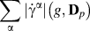 $\sum\limits_{\bf{\alpha }} {\left| {{{\dot{\gamma }}^\alpha }} \right|\left( {g,{{\bf{D}}_p}} \right)}$ needed for strain hardening or the plastic spin rate Wp(g, Dp) needed for texture evolution. The SCP approach was able to accelerate the CP calculations by approximately two orders of magnitude compared to the conventional NR-based approach.Reference Knezevic, Al-Harbi and Kalidindi124,Reference Al-Harbi, Knezevic and Kalidindi125
B. High performance computer hardware
Gains in computational efficiency in CP modeling have been demonstrated via exploiting the latest advancements in high performance computer hardware.Reference Mihaila, Knezevic and Cardenas133–Reference Mellbin, Hallberg and Ristinmaa135 Recent examples include adopting a computing architecture based on graphic processing unit cards (GPUs).Reference Knezevic and Savage136 While modern central processing units (CPUs) utilize more cores and wider SIMD (single instruction multiple data) units, running high performance super computers made up of merely CPUs is power intensive. Over the past decade, physical and engineering practicalities involved in microprocessor design have resulted in flat performance growth for traditional single-core CPUs. Additional performance gain has been primarily achieved through multicore designs and increased use of data parallelism. At the forefront of parallel computing are GPUs, originally developed for 3D visualizations and optimized for parallel processing of millions of polygons with very large datasets. Graphic workloads contain tremendous amounts of inherent parallelism. GPUs are considerably faster in comparison to CPUs for reading a large dataset. For example, the memory bandwidth on a Nvidia Tesla K80 GPU is up to 480 GB/s, while it is no more than 68 GB/s for systems with PC3-17000 DDR3 modules and quad-channel architecture. In terms of computational power, Tesla K80 is capable of achieving up to 2.91 and 8.74 TFLOPS for double precision and single precision, respectively, while it is no more than 900 GFLOPS for an Intel Xeon CPU E5-2699 v4 @ 2.20 GHz with 22 cores when using AVX2 and FMA3 instructions with the turbo boost enabled. Furthermore, GPUs are cost effective in comparison to CPUs, and a simple “off-the-shelf” GPU can significantly enhance the computational capabilities of desktop workstations. More importantly, GPU-ported software applications are growing at a rapid pace to address industrial and academic demands for massively parallel computing in quantum calculations (e.g., NWChem software), molecular dynamics (NAMD, GROMACS, AMBER software), FE calculations (Abaqus), and polycrystal plasticity simulation tools. Moreover, GPUs are uniquely suited for high-resolution visualization and analysis of large computational datasets (e.g., VMD software).
C. Hybrid methods
The aforementioned three basic ways for speeding up computation are not mutually exclusive, and thus, exploiting two or all three is a viable option. For instance, the multilevel toolset can be still computationally intensive and possible speed up could be realized by employing the SCP approach and a computing architecture based on GPUs. In this final section, a strategy of embedding SCP within implicit FE is first demonstrated with two case studies and afterward, a possible method for performing future computationally efficient PMP evolution simulations is motivated.
1. FE-SCP examples
Recently in Refs. Reference Zecevic, McCabe and Knezevic11, Reference Zecevic, McCabe and Knezevic49, and Reference Alharbi and Kalidindi137, the SCP model was incorporated into the implicit FE framework. In one study, the FE-SCP model was applied to calculate texture gradients that develop during the equal channel angular extrusion (ECAE) of Cu. ECAE is a severe plastic deformation technique that imposes large and nonmonotonic strains, resulting in texture gradients from the surface to the center of the billet. Figure 14(a) shows the setup for the FE-SCP simulation of ECAE. The deformed mesh after ECAE displaying the equivalent plastic strain contours (PEEQ) is shown in Fig. 14(c). The nonuniformity in the strain contours between the top and bottom of the extruded billet is a direct consequence of heterogeneous deformation history. The figure also shows the predicted textures at three different locations in the billet: top, middle, and bottom, in good agreement with experimental measurements reported in Ref. Reference Beyerlein, Li, Necker, Alexander and Tomé138.
(a) Initial mesh of the billet and analytical rigid rounded die geometry for the ECAE simulation per experiments reported in Beyerlein et al. 2005.Reference Beyerlein, Li, Necker, Alexander and Tomé138 (b) Initial mesh of the plate and analytical rigid top roll curvature for the rolling to a reduction of 50%. The cylindrical billet was meshed using 1040 C3D8 (continuum 3D eight nodal) elements. The plate was meshed using 396 CPE4 (continuum plane strain four-node elements). (c) Equivalent plastic strain contours predicted by the FE-SCP model. {111} pole figures showing predicted texture after ECAE at the three material points in the top, middle, and bottom of the die channel. (d) Equivalent plastic strain contours as predicted by the FE-SCP model on the left and the FE-VPSC model on the right. Corresponding {111} pole figures showing predicted texture after rolling at two polycrystalline material points as described in the figure. Reprinted with permission from Ref. Reference Zecevic, McCabe and Knezevic49.

In another study, the utility and computational speed up of the FE-SCP model is demonstrated for predicting texture gradients in the rolling of a BCC Haynes 25 alloy [Fig. 14(b)]. Figure 14(d) shows the PEEQ contours on the deformed mesh after rolling to 50% reduction. To highlight the quality and speed of the FE-SCP model, the texture predicted by the FE-SCP model and those predicted by an FE-VPSC model are compared in the figure. Both models capture the consequences of friction between the contacting rolls and plate surfaces, such as the localized shearing near the surface when exiting the rolls, and both produce similar textures after rolling. On the same workstation, the FE-VPSC model required 32.2 h, whereas the FE-SCP model required 1.2 h, indicating the outstanding speed up via the FE-SCP method.
2. Three-prong approach
It is envisioned that increased computational efficiency can be gained by implementing the foregoing FE-SCP framework onto graphics hardware. Figure 15 presents one possible hybrid CPU-GPU computational platform for FE-SCP intended for performing a microstructure-sensitive metal processing simulation, such as rolling. The platform shown considers a computer cluster, consisting of Linux nodes that individually integrate GPUs and CPUs. Starting from the bottom of the figure, the calculations are distributed such that the grain-level computing is performed on GPUs since GPU cards have thousands of cores achieving teraflop performance. In scaling up to the next level of the polycrystalline aggregate, the mesoscale homogenization is performed on the CPUs of individual slave Linux nodes. For a multiphase case, the polycrystalline aggregates may represent different domains in the FE model. Last, at the highest level, the master Linux node calculates the macroscopic component level response. Parallelization using only CPUs without GPUs is also possible; however, a cluster integrating many CPUs is significantly more computationally expensive than a computer workstation integrating GPUs.
Possible multilevel CP FE calculations distributed on a hybrid CPU-GPU computer architecture.

V. CONCLUSIONS
Over the years, mesoscale materials modeling approaches have been built to elucidate the role played by the microstructure, e.g., grain shape, grain orientation, grain size, internal grain boundaries, and interfaces, in PMP relationships of polycrystalline materials. Many high-performance polycrystalline materials of intense interest for future engineering applications are inherently or microstructurally complex, warranting advancements in such mesoscale deformation models beyond the standard versions. This article aims to highlight the latest developments in three-dimensional, mesoscale CP-based modeling techniques and the challenges they have overcome. In particular, some recent advancements in the ability to model the role that mesoscale microstructural features, such as grain (orientation, size, and shape), grain boundary, and interface properties, play in the development of local stresses states and deformation mechanisms during mechanical processing or straining are described and discussed. Examples cover studies that have used and extended mesoscale 3D, full-field spatial resolved computational models to investigate processing–microstructure relationships in boundary-dominant materials. These include examining the influence of strain and stress fluctuations at grain boundaries on the onset of deformation twinning or shear banding, and influence of bimetal interfaces on microstructural evolution.
ACKNOWLEDGMENTS
The authors gratefully acknowledge support from the U.S. National Science Foundation (NSF) under Grant Nos. CMMI-1728224 (UCSB) and CMMI-1727495 (UNH).