I. INTRODUCTION
Growing demand for high-speed wireless networks has led to the development of new, more sophisticated radio interfaces. In particular, multi-antenna (MIMO) technology has recently emerged to increase system performance while limiting spectral resource utilization [Reference Gesbert, Shafi, Da-shan, Smith and Naguib1, Reference Goldsmith, Jafar, Jindal and Vishwanath2]. As with any other modern radio interface, development, testing, and evaluation of MIMO systems involve extensive computer simulations. Accurate and reliable propagation channel models are therefore required to obtain coherent results from the entire simulation chain [Reference Almers3]. Modeling is always preceded by propagation channel characterization. In fact, channel models cannot be defined without the physical understanding of the measurement data. For example, Landmann et al. [Reference Landmann, Sivasondhivat, Takada, Ida and Thomä4] and Laurila et al. [Reference Laurila, Kalliola, Toeltsch, Hugl, Vainikainen and Bonek5] present characterization results in urban areas, such as the identification of reflection/diffraction/diffusion by buildings. However, the physical interpretation of measurements is sometimes long and laborious. Simultaneous comparison of measurement results, measurement campaign notes, building or city maps and standard photographs is time consuming and can be a source of error. The development of efficient and simple measurement analysis tools is therefore a concern for scientists involved in propagation channel characterization.
Mixing measurement results with environment photographs is certainly the most convenient way to physically analyze propagation channel behavior. In 2002, photographs taken with a standard lens onto which representative rays detected by the SAGE algorithm were superimposed were included in [Reference Fleury, Jourdan and Stucki6]. More recently, a method based on panoramic images generated from six video streams was presented in [Reference Kwakkernaat, de Jong, Bultitude and Herben7]. Omnidirectional video data that were captured during the measurements were used in combination with the measurement results to identify and relate the received radio waves directly to the actual environment. Both analyses were limited to the campus environment with large building separation.
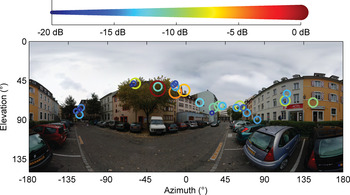
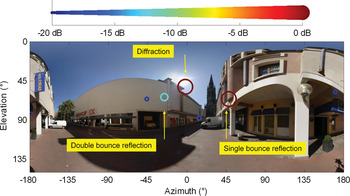
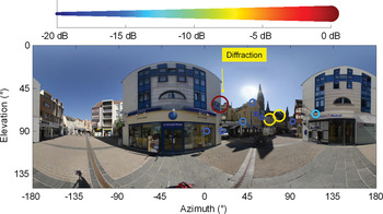
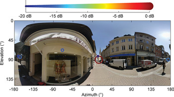
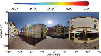
The purpose of this paper is to extend the previous analyses for real urban macrocell environments. The physical interpretation will be based on radiophotos which are defined as the superimposition of three-dimensional (3D) panoramic photos, with directions of arrival at the mobile. 3D panoramic photos are images with an angle of view that reaches 180° vertically and 360° horizontally. A radiophoto example is given in Fig. 1. The 0° azimuth axis represents the base station–mobile station (BS-MS) line. Each path is represented by a circle, the radius, or color of which is proportional to its power.
Radiophoto example.

The paper is organized as follows: Section II describes the measurement campaign and the estimation method for the directional propagation channel. An original method based on radiophotos is applied in order to detect and suppress the noise in the azimuth–elevation domain. Section III shows a large collection of radiophotos highlighting the main physical phenomena involved in the propagation channel in outdoor urban environments. Section III also provides radiophotos related to typical measurement files. The typical file selection was achieved according to the azimuth, elevation, and delay spread values.
II. MEASUREMENT DATA
A) Measurement campaign description
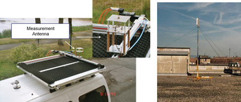
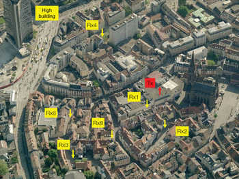
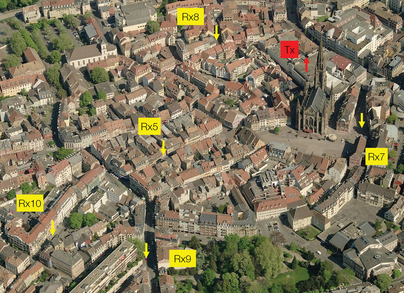
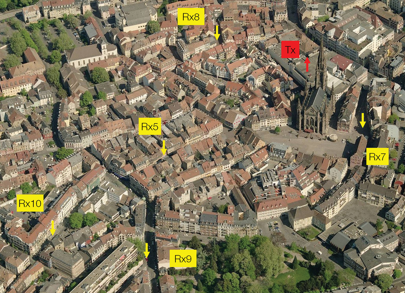
The measurement campaign was conducted in the city center of Mulhouse, France, where the average height of buildings is about 25 m. The propagation channel complex impulse responses (CIR) were collected with the wideband channel sounder of Orange Labs (AMERICC) [Reference Conrat, Pajusco and Thiriet8] at a carrier frequency of 2.2 GHz and a measurement bandwidth of 62.5 MHz. The Tx antenna was placed on the rooftop of a building at about 30 m above ground level. The Tx antenna was a 12 dBi gain sectorial antenna with a half power elevation beamwidth of 16°. The transmitted power was 43 dBm. Figures 3 and 4 show the urban environment viewed from the BS. At the receiver side, a static reference antenna and a virtual uniform planar array (VUPA) of 21 × 21 omni-directional dipole antennas were located on the roof of a car (Fig. 2). The signal coming from the reference antenna was used for time and phase synchronization. The synchronization procedure is detailed in [Reference Dunand and Conrat9, Reference Conrat, Dekov, Liénard and Abdelmottaleb10]. The Tx and Rx antennas were dual polarized; however, this paper deals only with the results in vertical polarization. A polarization statistical analysis based on this measurement campaign is presented in [Reference Dunand and Conrat11]. Rx1–Rx10 in Figs 3 and 4 indicate some Rx locations, the measurement results of which will be discussed in the following next sections.
Receiving and transmitting antennas.

BS aerial view 1.

BS aerial view 2.
B) Beamforming processing
A Bartlett beamforming algorithm is used to compute the various directions of arrival at the receiver. The general principle is to synthesize a narrow-beam antenna and scan the environment in all directions. The beamforming algorithm is applied at each delay and the final result is the directional impulse response h(θ, φ, τ), where θ, φ, τ are the elevation, the azimuth, and the delay, respectively. h(θ, φ, τ) is computed by applying the following formula:

where h mn(τ) is the impulse response at position (m, n) in the VUPA; G BS is the Tx antenna gain in the Tx–Rx direction; G MS(θ, φ) is the Rx antenna gain in the direction (θ, φ); B mn(θ, φ) is the antenna array response in the direction (θ, φ); W mn is the weighting function; NbAntRow is the VUPA row number; and NbAntLine is the VUPA line number. For the described campaign, NbAntLine = NbANtRow = 21.
W mn is a 2D weighting function which reduces the sidelobe level. The amplitude normalization complies with the following condition: if the VUPA is impinged by a ray with an amplitude A and a direction (θ, φ), the amplitude estimated by the beamformer in direction (θ, φ) is A. Results presented in the next sections use the Hanning function.
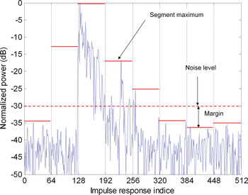
The beamforming algorithm is limited to a delay interval that includes CIR non-noisy parts. The noise level is estimated with the minimum of the maximum (MinMax) method illustrated in Fig. 5. The CIR is divided into N segments. P maxi is the maximum power over segment i. The noise level P noise is equal to

margin compensates the possible difference between the MinMax value and the maximum of noisy segments. The segment number and the margin are manually evaluated from a few CIRs and then applied to all CIRs. The MinMax method is simple and efficient but assumes that a sizeable part of the impulse response is noise. This assumption is usually checked as channel sounder excitation sequences are selected much longer than the expected maximal CIR length. A MinMax method adaptation in the azimuth–elevation domain is presented in Section II(C).
Impulse response noise estimation with eight segments.

The VUPA horizontal planar symmetry introduces an up/down ambiguity in the elevation estimation. From a strictly theoretical point of view, two rays with the same azimuth but with supplementary elevation angles cannot be resolved. Practically, the metallic plate, on which the XY-rail is set, shadows paths coming from the bottom. We can therefore assume that the measurement system is able to estimate without ambiguity elevations between 0 and 90°. Elevation 0° is the vertical direction.
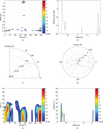
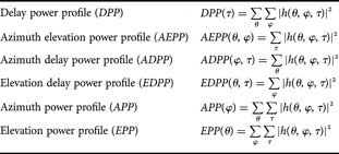
In order to visualize h(θ, φ, τ) clearly, different power profiles are defined as mentioned in Table 1. Examples of power profiles are shown in Fig. 6.
Power profiles computed from the directional impulse response, location Rx10: (a) ADPP, (b) DPP, (c) EPP, (d) APP, (e) AEPP, and (f) EDPP.

Profile definitions.

C) Channel discretization
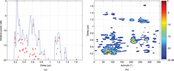
The discretization process involves finding the local maxima of |h(θ, φ, τ)|2 [Reference Conrat and Pajusco12]. h(θ, φ, τ) is converted in a set of ray defined by matrix Ray:

P i, τ i, θ i, and φ i are, respectively, the power, the delay, the elevation, and the azimuth of the ith ray. The method is illustrated in Fig. 7.
Path estimation via local maxima detection. Estimated paths are plotted with red crosses on the DPP plot and with dark points on the ADPP plot: (a) DPP and (b) ADPP.

This new representation has several advantages. It dramatically reduces the size of data structures used for saving the results, the computational complexity of successive operations and therefore the computational time. On the other hand, retaining only the peak values from the continuous profiles intrinsically ignores the width of the beamformer main lobe (along the angular dimension) and the measurement equipment rise time (along the temporal dimension).
The noise level determination is a crucial step in the channel estimation method described above. The noise includes all undesirable signals due to thermal noise, beamforming sidelobes, measurement equipment limits, or channel non-stationarity. Regarding the path estimation process described in the previous paragraphs, the noise level defines a threshold above which local maxima detected on power profiles are not considered as physical paths. Its minimal value is theoretically bounded by the estimator space–time sidelobes. The directional impulse response was computed using a Hanning function. Therefore all maxima, the power of which is lower than the maximal power minus 30 dB, are withdrawn from the estimation. Its maximal value depends on the measurement conditions and is calculated for each impulse response delay by the MinMax method extended in the azimuth–elevation domain.
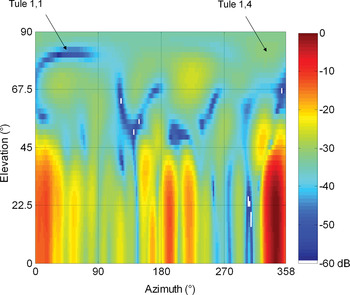
For each delay, h(θ, φ, τ) is divided into N elev × N azi tules as shown in Fig. 8. The noise level P noise_minmax(τ) is processed according to equation (4). P maxi, j is the maximum of |h(θ, φ, τ)|2 over tule i, j at delay τ:

Tule division example.

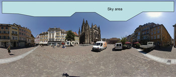
As pointed out in Section II(B), the MinMax method is efficient if N elev, N azi, and margin are correctly calibrated from a few measurement samples. The calibration involves comparing P noise_minmax(τ) with a noise reference value called P noise_ref(τ) and calculated using radiophoto. The method is based on two basic assumptions: Firstly, receiving power from the sky is physically impossible. There can be obstacles above the vehicle momentarily, but the obstacle shadowing elevation is practically always lower than the building shadowing elevation, as shown in Fig. 9. Secondly, the noise is statistically not dependant on the direction of arrival. A sky area is defined inside a panoramic photo where no signal can be received. The maximum power within the sky area gives P noise_ref(τ).
Sky area example.

The optimal values for N elev, N azi are those that minimize the peak-to-peak value of P noise_minmax(τ) − P noise_ref(τ). Typical N elev, N azi, and margin values are, respectively, 4, 4, and 10 dB. Performance of noise estimation methods is illustrated in Fig. 10. The curve denoted Max is equal to the maximum of |h(θ, φ, τ)|2 at delay τ. The curve denoted MinMax is P noise_minmax(τ) minus margin. The directional impulse response depicted in Fig. 8 was computed at delay 0.28 μs.
Noise estimation as a function of delay, N elev = 4, N azi = 4, and margin = 10 dB.

The accuracy of the path estimation method was evaluated by selecting measurement points in line-of-sight condition. The main path is defined as the path with the lowest attenuation. As there is no obstacle between Tx and Rx, the main path is the direct path between Tx and Rx. The main path direction was compared with the direction computed from the Rx and Tx coordinates and the main path attenuation was compared to the free space loss attenuation. The angular difference is less than 5° and the attenuation difference is less than 4 dB. The angular difference is not significant as it depends on the Tx and Rx coordinate accuracy as well. The attenuation difference is explained by the addition of small errors on the Tx power, antenna gains, or cable losses, but it is impossible to characterize all sources of error separately. Nevertheless, even though the path estimation may be locally biased, the measurement data and estimation process are sufficiently accurate and reliable for understanding the physical phenomena of the propagation channel.
D) Radiophoto generation
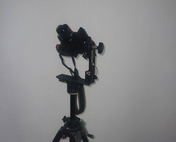
Panoramic photography is a style of photography that aims to create images with wide fields of view. When the angle of view reaches 180° vertically and 360° horizontally, panoramic photos are called 3D panoramic photos. The easiest way to obtain such photos is the stitching method. The principle is to take a set of photographs that overlap slightly and to stitch them with specific software. The main drawback is the relatively long acquisition time, about 10 min, which prohibits all real-time applications. However, consumer products can be used. Therefore, the stitching method is the most widely used and a lot of information related to the equipment or software is available on the web. The equipment is composed of a conventional digital camera, a fish-eye lens, a tripod and a panoramic head. The fish-eye lens is a very wide-angle lens. The panoramic head is mounted on a tripod (Fig. 11) and has two functions: to set the axis of rotation precisely and to rotate the camera in 3D. Panoramic photography is performed in three steps:
– Panoramic head setting: The panoramic head should be set to match up the entrance pupil of the lens (optical focalization point) with the rotation center of the panoramic head. An accurate setting avoids parallax errors and makes image stitching easier. The entrance pupil is located on the lens rotation axis but its exact location is unknown, as lens manufacturers refuse to disclose these data, deeming it confidential. Fortunately, there are very simple methods to adjust the panoramic head.
– Photo acquisition: First, the number of photographs needed to cover the selected area is calculated. This number depends on the lens angular aperture and on the overlapping rate. The overlapping rate indicates the percentage of common field of view between two consecutive pictures. It is generally considered that an overlapping rate of about 20–25% makes correct stitching possible. As a next step, photographs are shot. In real environments, the light level changes greatly and photographs taken into the sun tend to be over-exposed. In this case, increasing the overlapping rate helps the stitching software to generate a panoramic photo with uniform brightness.
– Picture stitching and panorama export: The quality of this step depends heavily on the software. We used Stitcher Unlimited software that performs all operations automatically and efficiently. The most time-consuming parts of the processing are image stitching between neighboring pictures and brightness smoothing. Once these operations are completed, the panoramic photography is generated according to a user-defined projection system. We used spherical projection, where the X-axis is proportional to the azimuth and the Y-axis proportional to the elevation.
Camera set on the panoramic heading.

Figure 12 gives an example of 24 shots at two elevations (0 and 45°) and 12 azimuths (30° step). The overlapping rate is 50% horizontally and 70% vertically. This configuration leads to a panoramic photograph with a 360° horizontal angle of view and 155° vertical angle of view.
Set of photographs taken with the fish-eye lens.

III. PHYSICAL ANALYSIS OF THE PROPAGATION CHANNEL
Locations Rx1–Rx10 are depicted in Figs 3 and 4.
A) Propagation mechanisms
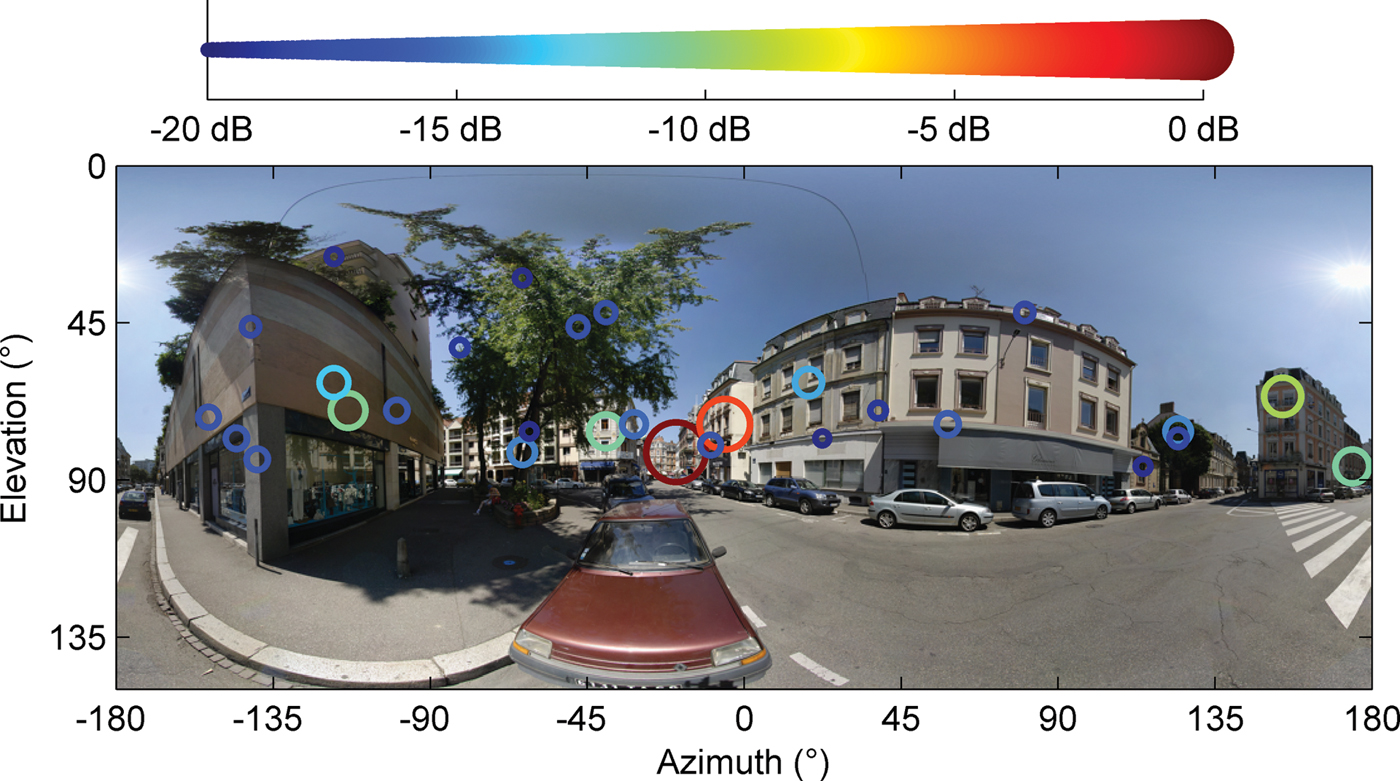
Location Rx1 as shown in Fig. 13 highlights two basic phenomena of electromagnetic wave propagation in outdoor environments: the reflection on building walls and the diffraction at horizontal building edges. Vertical building edges can also diffract the electromagnetic wave (Fig. 14), although this phenomenon is less frequent in macrocell environments where the transmit antenna is well above the rooftop level.
Radiophoto location Rx1.

Radiophoto location Rx2.

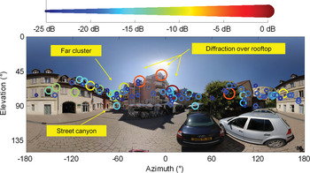
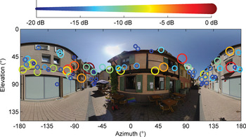
The first two examples were simple cases as the preponderant paths impinging the MS undergo less than two phenomena. Location Rx2 as shown in Fig. 15 shows a much more complex case and illustrates the different propagation mechanisms that have also been described in [Reference Conrat and Pajusco13–Reference Kuchar, Rossi and Bonek16].
Radiophoto location Rx3.

Diffraction over rooftops: Waves arrive at the MS from the rooftop level by diffraction at roof edges. The direction of arrival is generally close to the BS–MS direction, the elevation may be high if the receiver is located near the wall of the building and the relative delays are short.
Street-guided propagation: Waves arrive at the receiver at street level after traveling through street canyons by bouncing off walls along the street. Elevations associated with this mechanism are generally close to 90°.
Far scatterer reflection: Waves arrive at MS after reflection off a building whose height which greatly exceeds the average rooftop level. A delay of about a few μs may be observed.
Miscellaneous: Other cases include reflection or diffraction on buildings or objects surrounding the MS.
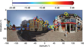
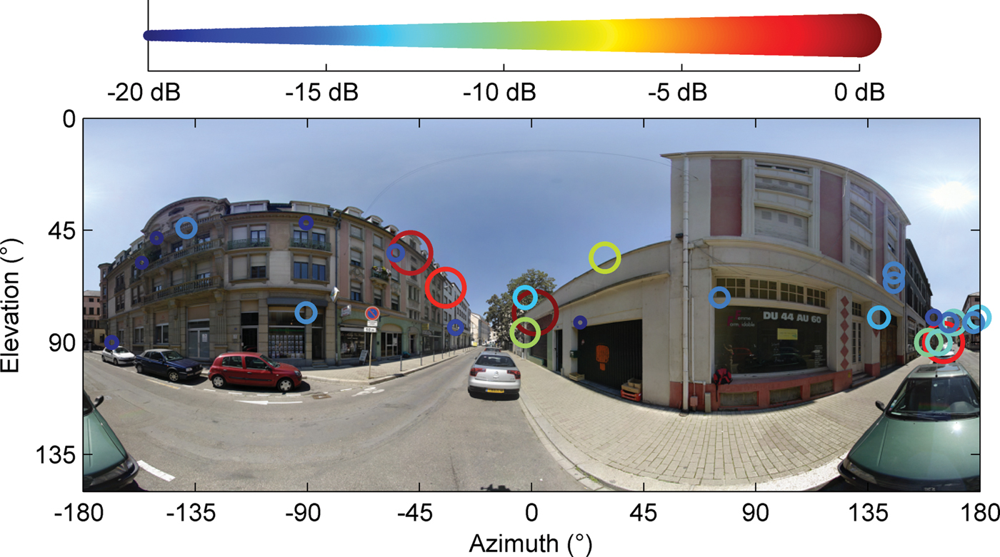
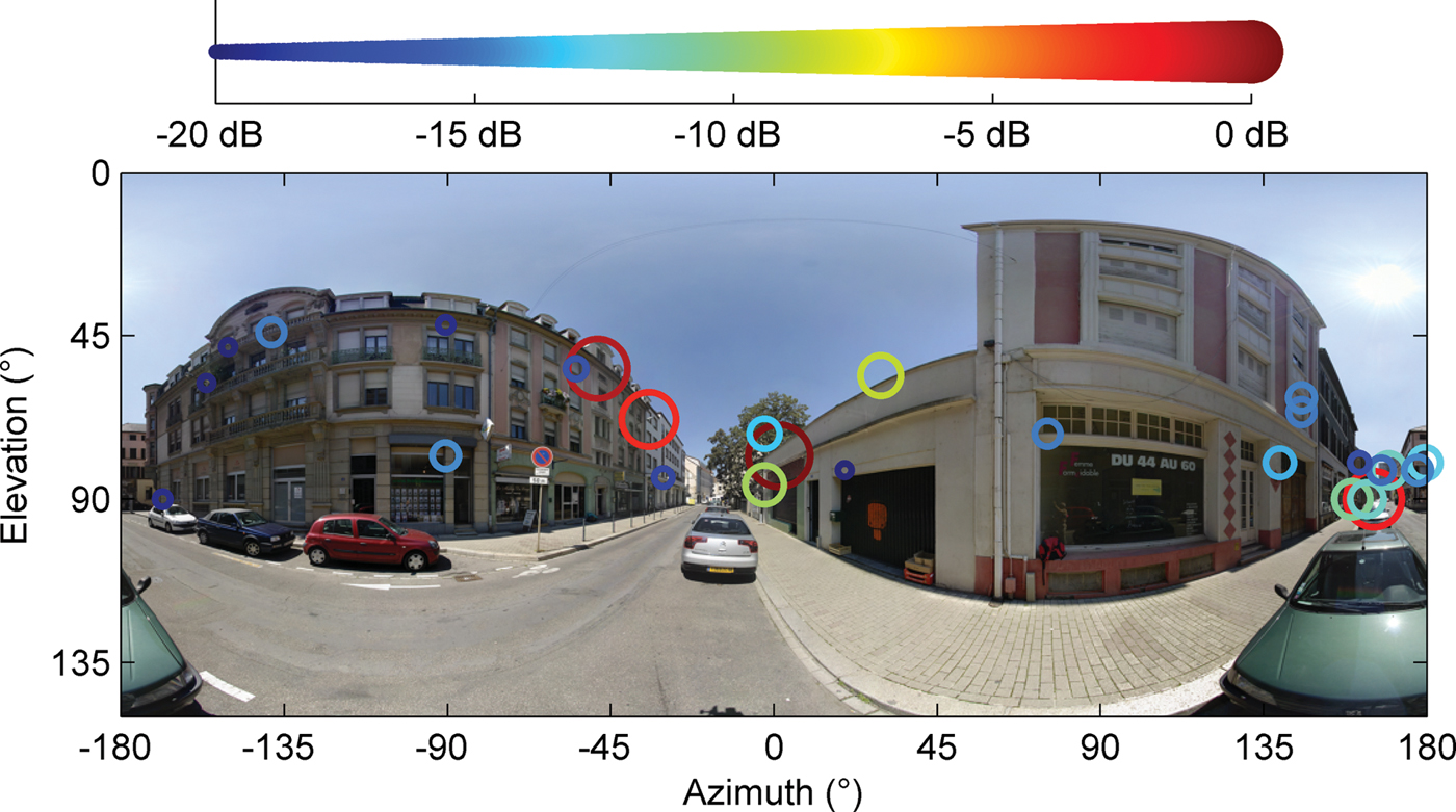
When the street axis corresponds to the BS–MS direction, the street canyon effect is enhanced as the different propagation mechanisms described above are combined to increase the received power in the street axis as shown in Fig. 16. Similar results were reported in [Reference Conrat and Pajusco13].
Radiophoto location Rx4.

B) Typical propagation channels in an urban environment
Typical measurement files are selected according to the azimuth spread at mobile (AS), the elevation spread at mobile (ES), and the delay spread (DS). AS and ES indicate the spatial diversity degree of the propagation channel. DS indicates the frequency diversity degree. AS, ES, and DS are key parameters for propagation channel characterization and modeling [17]. Therefore, they are appropriate channel metrics to identify typical propagation channels. AS, ES, and DS are processed from the discrete representation of the continuous function h(θ, φ, τ). Only rays within a dynamic range of 20 dB are considered in spread processing. P i, τ i, θ i, and φ i are the power, delay, elevation, and azimuth of the ith ray, respectively.
DS and ES are calculated using


AS is calculated according to equation (7) and complies with the 3GPP specification [18]
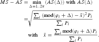
mod designed the modulo-2π function.
The minimum and maximum spread values are analytically calculated in the case of an equally powered azimuth distribution ranging in the interval [0, α]. Spread values ranged from 0 to  . For instance, AS ranges from 0 to 104° and ES ranges from 0 to 28°.
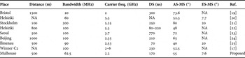
Before the typical measurement file selection itself, AS, ES, DS mean values are compared with those extracted from similar measurement campaigns and reported in Table 2. The carrier frequency ranged between 2 and 6 GHz and the measurement setup enabled direction of arrival estimation at MS. The environment was the outdoor macrocell environment and corresponds to scenario C2 defined by the WINNER European project [17]. Results are almost homogeneous, despite the fact that measurements have been performed in different European or Asian cities with a specific architecture or urban density. With the exception of extreme values, DS mean values range from 100 to 300 ns, AS mean values are between 50 and 70°, and ES is about 8°. Therefore, typical propagation channels described below are not strongly specific to the measurement campaign environment and may be generalized to many types of urban areas.
Measurement campaign summary.

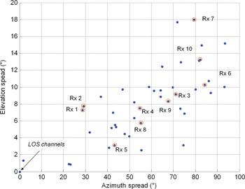
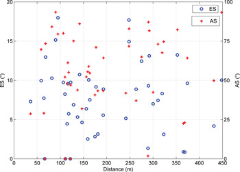
The typical propagation channel selection was done manually and based on a simple observation as shown in Fig. 17: ES and AS are correlated, thereafter the measurement points may be classified according to their spatial diversity degree at MS. Three typical channels were defined: “Quasi-LOS”, “High spatial diversity”, and “Standard”. The first two typical channels are extreme cases that represent roughly 30% of the measurement points. Furthermore, typical channels are not associated with the BS–MS distance. This statement is motivated both by the joint radiophoto and aerial view visual inspection and by the low correlation between the BS–MS distance and AS or ES illustrated by Fig. 18.
AS versus ES.

AS or ES relation with distance.

Channel “Quasi-LOS” ( Fig. 19): Propagation channels are usually classified as either LOS (line-of-sight) or NLOS (non-LOS). Strictly speaking, LOS conditions mean that the transmitter is visible from the receiver. Channels with pure visibility are very rare in real urban environments but many situations classified as quasi-LOS have characteristics similar to LOS: a predominant path with a direction close to the BS–MS line and weakened secondary paths less than 10 dB below the predominant path. The street axis generally has the same orientation as the BS–MS line. Delay spread values are centered around 30 ns and do not exceed 100 ns. AS ranges between a few and 50°, depending on the secondary path azimuth.
Radiophoto location Rx5.

Channel “High spatial diversity” ( Fig. 20): The strongest path propagates less than 20% of the total received power. Some files exhibit a relatively high elevation spread. This ccurs when two conditions are met, as shown in Fig. 21. Firstly, either a high building is in the vicinity of the MS or the MS is close to the building wall. This geometrical configuration creates paths with an elevation ranging roughly between 40 and 70°. Secondly, a significant part of the power arrives at MS with a low elevation. The addition of paths with low and large elevation creates ES close to 20°.
Radiophoto location Rx6.

Radiophoto location Rx7.

Channel “Standard”: Except for some files that exhibit enhanced street canyon behavior as described in Section (A), it is impossible to refine the selection as each measurement point is a particular case. Figures 22 and 23 are two examples.
Radiophoto location Rx8.

Radiophoto location Rx9.
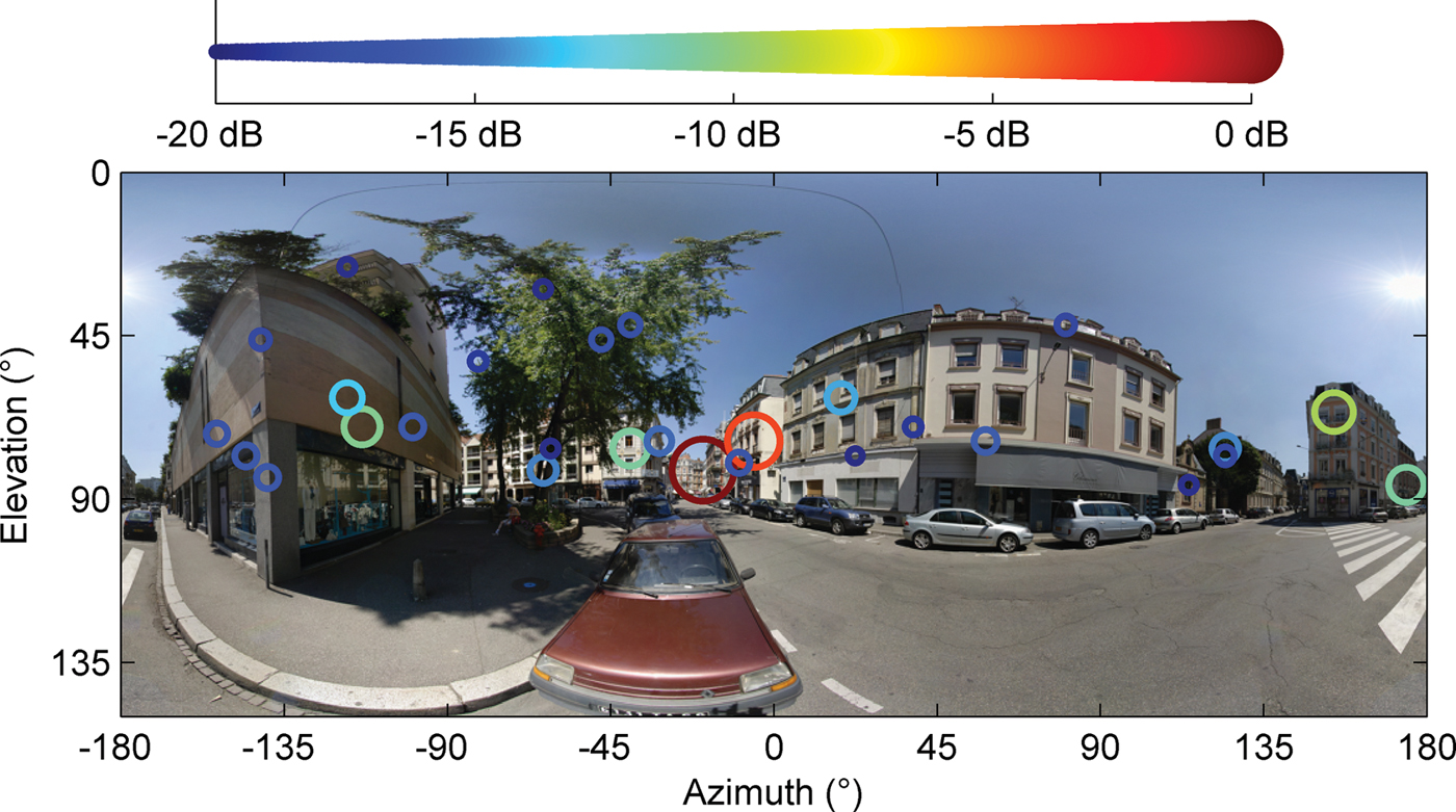
The groups “High spatial diversity” and “Standard” have the same mean DS value around 200 ns. Most of the DS are between 30 and 400 ns, but some files exhibit very large DS between 500 and 700 ns. This usual situation occurs when the impulse response is divided into two discontinuous parts as shown in Figs 24 and 6. The first part is due to the interaction of the electromagnetic wave with the environment in the vicinity of the MS or close to the BS–MS line. The second part is generally an interaction with a faraway building and generates paths with excess delay higher than 1.5 μs. This type of file agrees with environment C3 defined by the Winner project and labeled as “macro-cell bad urban”.
Radiophoto location Rx10.
IV. CONCLUSION
The radiophoto examples given in this paper have shown the huge potential of radiophotos for data validation and analysis of propagation measurements. In particular, the impact of the environment on the space–time propagation channel is immediately identifiable. Future work based on this technique will focus on the validation of simulation techniques, such as ray tracing or ray launching. Simulation results will be added to radiophotos, which should improve our understanding of the influence of geographical database accuracy on simulation reliability.
APPENDIX
Radiophotos do not provide any information about the path relative delay due to the intrinsic nature of the panoramic photo. However, the radiophoto principle can be extended to the video domain by generating radiovideos that show the AEPP time evolution dynamically. Radiovideos are multimedia documents that cannot be inserted in a journal paper but radiovideos related to the radiophoto examples given in this paper are available at http://perso.telecom-bretagne.eu/patricepajusco/jmwt/.
 Jean-Marc Conrat was born in Nancy, France, in 1968. He received his M.S. degree in electrical engineering from the National Institute of Applied Sciences (INSA), Lyon, France, in 1991. Since 1993, he has been with Orange labs in Belfort, France. He is involved in propagation channel measurements, modeling, and simulation. He started on wideband propagation channel studies for Land Mobile Satellite Systems (GLOBALSTAR). In 1996, he worked on the development of a new wideband channel sounder and was particularly involved in the software and digital aspects of this project. His current research interest is the characterization of the directional wideband propagation channel for terrestrial MIMO and cooperative communications.
 Patrice Pajusco received his engineering degree from the Ecole Supérieure d'Electricité (SUPELEC) in Paris, in 1992. He joined the France Telecom research center (CNET) in 1993, studying wideband propagation channel models for mobile communication systems and investigating wideband sounding techniques using antenna arrays. Starting in 1999, he was in charge of a team at Orange Labs working on propagation tools for wireless communication systems. In 2008, he joined Telecom Bretagne, where he is head of the microwave department. His main research interests are UWB and MIMO channel modeling.