I. INTRODUCTION
Modern communication and other applications require antennas having narrow beamwidth and large directivity which cannot be achieved by a single antenna. So, the design of antenna arrays has become a hot research area in recent years. Pattern synthesis of antenna arrays plays an important role in the design of antennas. The synthesis of antenna arrays is difficult because it is usually a high non-linear problem. As the development of radar and sonar, modern electronic system requires higher demands for the antenna arrays. So, classical analytic synthesis methods, such as Taylor synthesis method and Woodward–Lawson synthesis method [Reference Balanis1], are usually ineffective which has led to the use of global optimization methods. There are a variety of different global evolutionary methods that have been introduced into the synthesis of antenna arrays, such as genetic algorithm [Reference Haupt2], particle swarm optimization [Reference Pathak, Mahanti, Singh, Mishra and Chakraborty3, Reference Wang, Feng and Liu4], differential evolutionary (DE) [Reference Li, Li, Shi, Yang and Yu5], and invasive weed optimization (IWO) [Reference Chen, He and Han6]. These methods can usually obtain satisfactory results in the synthesis of antenna arrays.
Research on circular antenna arrays has become popular as they have the ability of scanning in all direction [Reference Panduro, Mendez, Dominguez and Romero7–Reference Ghosh, Banerjee, Das and Chowdhury10]. Compared with linear and rectangular arrays, circular antenna arrays are less sensitive to mutual coupling because they do not have edge elements [Reference Balanis1, Reference Singh and Kamal9]. So, synthesis of circular antenna arrays is paid more and more attention in recent years. Design of non-uniform circular array antennas for maximal side lobe level reduction with a fixed beamwidth is dealt with in [Reference Panduro, Mendez, Dominguez and Romero7]. In order to avoid the mutual coupling effects, intelligent optimization algorithm called IWO is presented in [Reference Roy, Das, Chakraborty and Suganthan8] for the design of various kinds of antenna arrays that can achieve minimum peak side lobe levels for a specific beamwidth. In [Reference Singh and Kamal9], biogeography-based optimization (BBO) is used into the design of non-uniform circular antenna arrays. Minimum side lobe levels for a specific first null beamwidth (FNBW) and also a minimum size of the circumference is achieved in [Reference Ghosh, Banerjee, Das and Chowdhury10] by an optimization design method for non-uniform, planar, and circular antenna arrays.
However, the methods proposed above cannot constrain the size of the antenna array and the minimum spacing of the adjacent array elements. A newly designed method is presented in this paper which can constrain the element number, size of the array, and adjacent elements spacing simultaneously. The element position and excitation amplitude of each element are optimized by HIWO and low peak side lobe level (PSLLs) of the radiation patterns are obtained. IWO has been widely used in the design of antennas [Reference Roy, Das, Chakraborty and Suganthan8, Reference Sedighy, Mallahzadeh, Soleimani and Rashed-Mohassel11–Reference Mehrabian and Lucas13]. Usually, IWO outperforms the other optimization methods in the convergence rate as well as the final error level. The rest of the paper is organized as follows: in Section II, the mathematical formulation is given. The used optimization algorithms are briefly described in Section III. In Section IV, numerical results and comparisons are given. Finally, the paper is concluded in Section V.
II. MATHEMATICAL FORMULATION
A) Geometry and array factor of circular antenna array
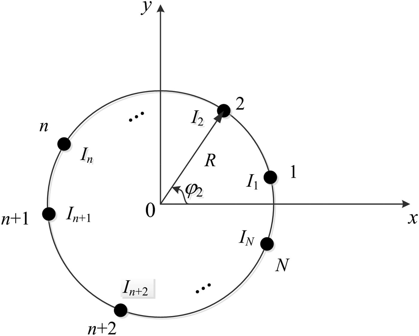
The structure of a circular antenna array with N elements is shown in Fig. 1. The radius of the circle is R. The array elements are arranged on the circle in x–y plane. The array elements are assumed to be isotropic sources. So, the array factor of this antenna array can be given by
 $$AF(\theta, \phi ) = \sum\limits_{n = 1}^N {I_n \exp (jkR\;\sin \theta \;\cos (\phi - \varphi _n ) + j\alpha _n )}, $$
where I n, α n are the excitation amplitude and phase of the n th element, φn is the angular position of the nth element, k = 2π/λ is the wave number and λ is the wavelength, θ and ϕ are elevation angle and azimuth angle, respectively. If only the array factor in x–y plane is considered, i.e. θ = 90o, the array factor can be depicted by
 $$AF(\phi ) = \sum\limits_{n = 1}^N {I_n \exp (jkR\;\cos (\phi - \varphi _n ) + j\alpha _n )}. $$
Structure of the circular antenna array.

If the direction of the main beam of the antenna array is ϕ 0, the excitation phase of the nth element can be given by
 $$\alpha _n = - kR\;\cos (\phi _0 - \varphi _n ).$$
B) Fitness function
In the design of antenna array, the PSLL, gain, and beamwidth of the radiation pattern are usually used to evaluate the fitness function. The purpose of this paper is to design antenna arrays with minimum side lobe levels. The FNBW is also not too large. So, the desired function can be given by
 $$E = w_1 \left. {\displaystyle{{\left \vert {AF(\phi )} \right \vert} \over {AF_{\max}}}} \right \vert _{\phi \in S} + w_2 SRR,$$
where w 1 and w 2 are weighting factors. AF max is the maximum value of |AF(ϕ)|.S is the side lobe area of the radiation pattern. SRR is the error of the calculated FNBW and desired maximum FNBW which can be defined by
 $$SRR = \left\{ {\matrix{ {0,\quad \quad {\rm if}\;FNBW_c \lt FNBW_d} \cr {FNBW_c - FNBW_d, \quad \quad {\rm elsewhere}} \cr}} \right.,$$
where FNBW c and FNBW d are the calculated and desired FNBW.
In order to avoid the overlap of array elements, the minimum spacing constraint of adjacent elements is depicted by d e. The range of the excitation is  $I_n\hat I{\rm [}I_{min},I_{max}{\rm ]}$. So, the objective function can be given by
 $$\left\{ {\matrix{ {min\left\{ E \right\}} \cr {s.t.\left \vert {\varphi _{i + 1} - \varphi _i} \right \vert \ge {{d_e} / R},\;I_{\min} \le I_n \le I_{\max.}} \cr {i = 1,2, \cdot \cdot \cdot, N - 1;\;n = 1,2, \cdot \cdot \cdot, N} \cr}} \right.$$
In the following procedure, the problem is changed into a maximum problem. So, the fitness function can be defined by
 $$f = \displaystyle{{1.0} \over {1 + E}}.$$
C) Optimization of excitation amplitudes and element positions
The excitation amplitudes of the array elements have minimum and maximum values which can be depicted by I min and I max, respectively. So, the excitation amplitude of the n th element can be calculated by
 $$I_n = I_{min} + (I_{max} - I_{min} ) \times r_n, \quad n = 1,2, \cdot \cdot \cdot, N,$$
where  $r_n \in [0,1],{\kern 1pt} \;n = 1,2, \cdot \cdot \cdot, N$.
As is shown in Fig. 1, the angular length of the circular antenna array is φL = 2π. If the minimum spacing constraint of the adjacent elements is d e, the minimum angular spacing of the adjacent elements can be calculated by
 $$\varphi _e = \displaystyle{{d_e} \over R}.$$
As the spacing between the first element and n th element cannot arrange other elements, the maximum angular length that can allocate array elements is φL − φe. If array elements are allocated by the minimum angular spacing constraint φe, the length of (N − 1)φe is occupied. So, the remaining region over the array aperture to be optimized is given by [Reference Chen, He and Han6]
 $$SP = \varphi _L - \varphi _e - (N - 1)\varphi _e = \varphi _L - N\varphi _e. $$
In the determination of element positions, the position of the first element must be determined. The first element should be allocated in the area of [0, SP]. So, the angular position of the first antenna array element can be depicted by
 $$\varphi _1 = SP \times r_{N + 1}, $$
where r N+1 is random number among the range of [0, 1]. Then, N − 1 real random numbers among the range of [0, SP] are calculated by
 $$c^{\prime}_{n - N - 1} = SP \times r_n, \;n = N + 2,\;N + 3, \cdot \cdot \cdot, 2N,$$
where r n, n = N + 2, N + 3, · · · , 2N are real random numbers among the range of [0, 1]. Then, c′i are sorted in ascending order and a new vector  ${\bf C} = [c_1, c_2, \cdot \cdot \cdot, c_{N - 1} ]$ is obtained, where c 1 ≤ c 2 ≤ · · · ≤ c N−1. The angular position of the n th element can be calculated by
 $$\eqalign{\left[ {\matrix{ {\varphi _2} \cr {\varphi _3} \cr { \cdot \cdot \cdot} \cr {\varphi _N} \cr}} \right] & = \varphi _1 + \left[ {\matrix{ {c_1} \cr {c_2} \cr { \cdot \cdot \cdot} \cr {c_{N - 1}} \cr}} \right] + \left[ {\matrix{ {\varphi _e} \cr {2\varphi _e} \cr { \cdot \cdot \cdot} \cr {(N - 1)\varphi _e} \cr}} \right] \cr &= \varphi _1 + \left[ {\matrix{ {c_1 + \varphi _e} \cr {c_2 + 2\varphi _e} \cr { \cdot \cdot \cdot} \cr {c_{N - 1} + (N - 1)\varphi _e} \cr}} \right].}$$
If φn >2π, φn is updated by
 $$\varphi _n = \varphi _n - 2\pi, \;n = 2,3, \cdot \cdot \cdot, N.$$
Then, φn is sorted in ascending order and the ultimate φn is obtained. It can be proved that the element angular spacing between n th element and (n + 1)th element is φe + (c n+1 − c n), n = 1, 2, · · · , N − 1 which satisfies the minimum spacing constraint of (6).
III. INTRODUCTION TO THE OPTIMIZATION ALGORITHM
A) Hybrid invasive weed optimization
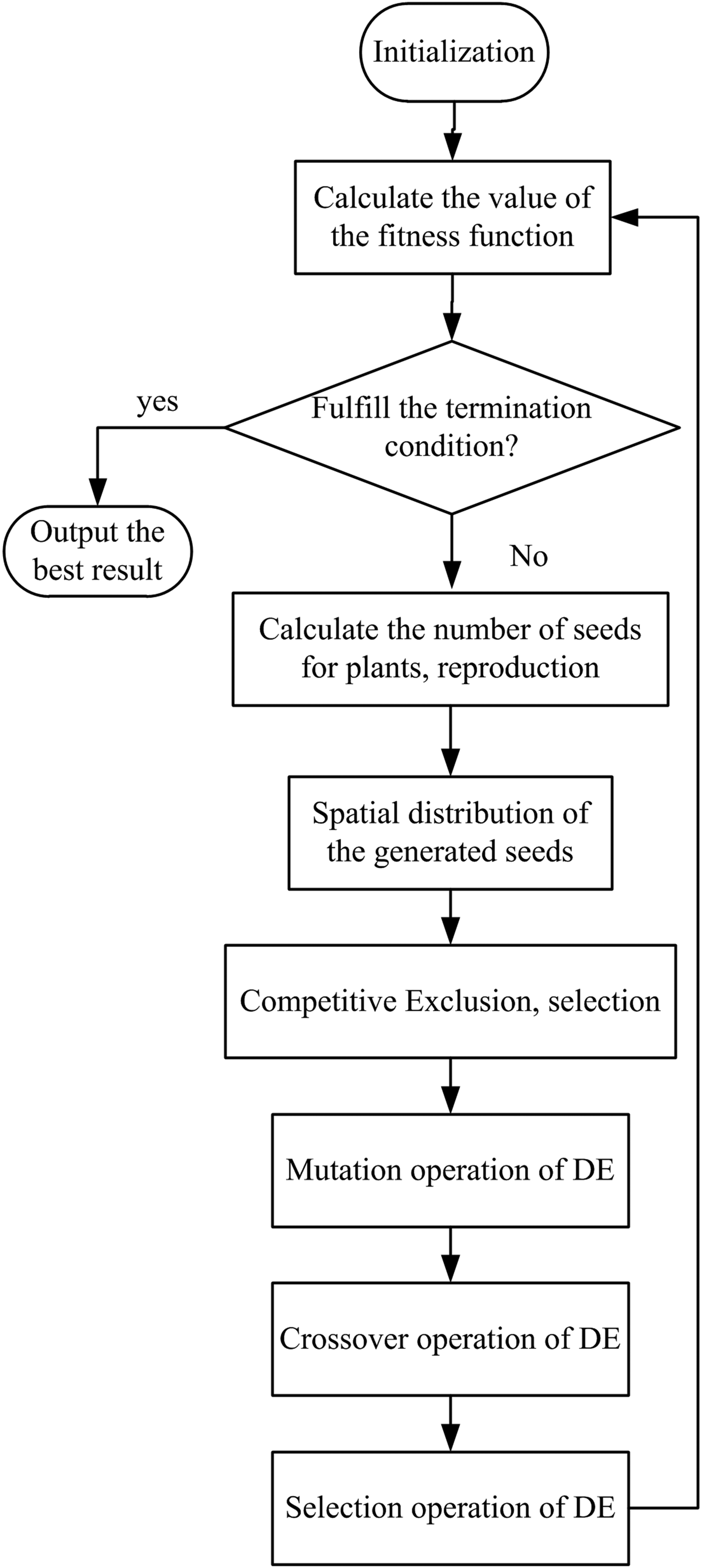
IWO and DE are effective intelligent optimization methods which have been widely used in the synthesis of antenna arrays [Reference Mehrabian and Lucas13–Reference Lin, Qing and Feng17]. Usually, these methods can obtain satisfactory results [Reference Guo, Guo and Ding15–Reference Lin, Qing and Feng17]. In order to improve the synthesis results, DE is embedded into the process of IWO which is called hybrid invasive weed optimization (HIWO). The flowchart of this hybrid optimization method is given in Fig. 2.
Flowchart representation of hybrid IWO.

B) Optimization steps
In order to optimize the positions and excitation amplitudes of the array elements using hybrid IWO, the optimization procedure can be expressed as follows:
Step 1. The parameter values of the antenna arrays and hybrid IWO are given. A 2N × P-dimensional matrix  ${\bf r}$ is chosen as the initial population to be optimized where
 ${\bf r} = \left[ {{\bf r}^1, {\bf r}^2, \cdot \cdot \cdot, {\bf r}^P} \right]$ and
 ${\bf r}^p = [r_1^p, r_2^p, \cdot \cdot \cdot, r_{2N}^p ]$. Each element of the matrix is depicted by
 $r_n^p \in [0,1]$, n = 1, 2, · · · , 2N, p = 1, 2, · · · , P. Let iter = 1. The first N elements of
 ${\bf r}^p $ are used to optimize the excitation amplitudes of the array elements. The last N elements of
 ${\bf r}^p $ are used to optimize the angular positions of the array elements.
Step 2. The excitation amplitudes and angular positions of the array elements are calculated by (8) and (13).
Step 3. The radiation patterns of the antenna arrays are calculated by (2). The fitness value is defined by (7) which increases with the decrease of PSLL. The optimized parameters that can produce the best fitness are preserved as the ultimate result.
Step 4. The optimization parameters  ${\bf r}^p $, p = 1, 2, · · · , P, are updated by HIWO which have been introduced in Section IIIA.
Step 5. Let iter = iter + 1, if iter <iter max, go to step 2, otherwise, terminate iteration.
IV. OPTIMIZATION RESULTS
In this section, three circular antenna arrays with 8, 10, and 12 elements are optimized. The range of the excitation amplitudes is I n ∈ [0.1, 1], i.e. I min = 0.1, I max = 1.0. If the radius of the circular antenna array is R, the minimum angular spacing of the adjacent elements is φe = d e/R. It can be found from (10) that small φe will increase the searching space of the algorithm which will affect the convergence rate of the algorithm. However, large φe will reduce the searching space of the algorithm which may lead to a poor synthesis result. So, a proper value of φe should be determined. After several calculations and referring some other papers [Reference Haupt2, Reference Chen, He and Han6, Reference Zhang, Jiao, Weng and Zhang16, Reference Lin, Qing and Feng17], the minimum spacing of the adjacent elements is chosen as d e = 0.5λ. The direction of the main beam is ϕ 0 = 0o. The weighting factor w 1 = w 2 = 1. The positions and excitation amplitudes of the array elements are optimized to get radiation patterns with low side lobe levels. So, the parameters that will be optimized can be depicted by
 $${\bf X} = [I_1, I_2, \cdot \cdot \cdot, I_N, \varphi _1, \varphi _2, \cdot \cdot \cdot, \varphi _N ].$$
The algorithm is calculated 10 times and the best result is preserved. As is depicted in [Reference Guo, Guo and Ding15, Reference Zhang, Jiao, Weng and Zhang16], the parameters used in HIWO are given in Table 1. The maximum and minimum numbers of seeds that can be produced in the algorithm process are s max and s min. The maximum and minimum standard deviations are σ max and σ min, respectively. The searching space is P and the maximum number of population is  $p\_\max $. The maximum number of iteration steps is iter max. The non-linear modulation index is represented by nmi. The scaling factor and crossover factor of DE are depicted by F and CR.
HIWO parameter values.

In order to show the effectiveness of the given method, the synthesis results calculated by IWO and DE are given. The parameters used in IWO are the same as HIWO. In the DE algorithm, the scaling factor and crossover factor are given in Table 1. In order to obtain satisfactory results, the maximum population of DE is set to be 150 [Reference Li, Li, Shi, Yang and Yu5].
The population size of HIWO is the same as IWO. Compared with IWO, HIWO will take much more algorithm time because a DE procedure is embedded into the progress of IWO. However, as the population size of IWO is much less than DE [Reference Li, Li, Shi, Yang and Yu5, Reference Guo, Guo and Ding15], HIWO needs much less population size than DE. DE algorithm also has a faster computational speed than IWO when the population size is the same. So, the additional algorithm time of HIWO is limited.
A) Optimization result of 8-element circular antenna array
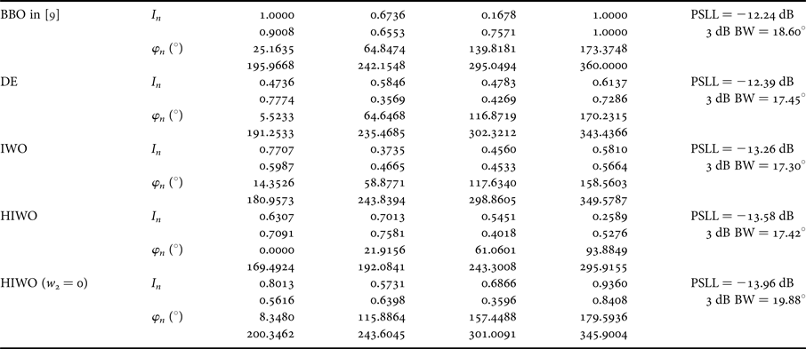
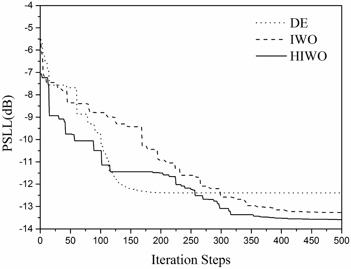
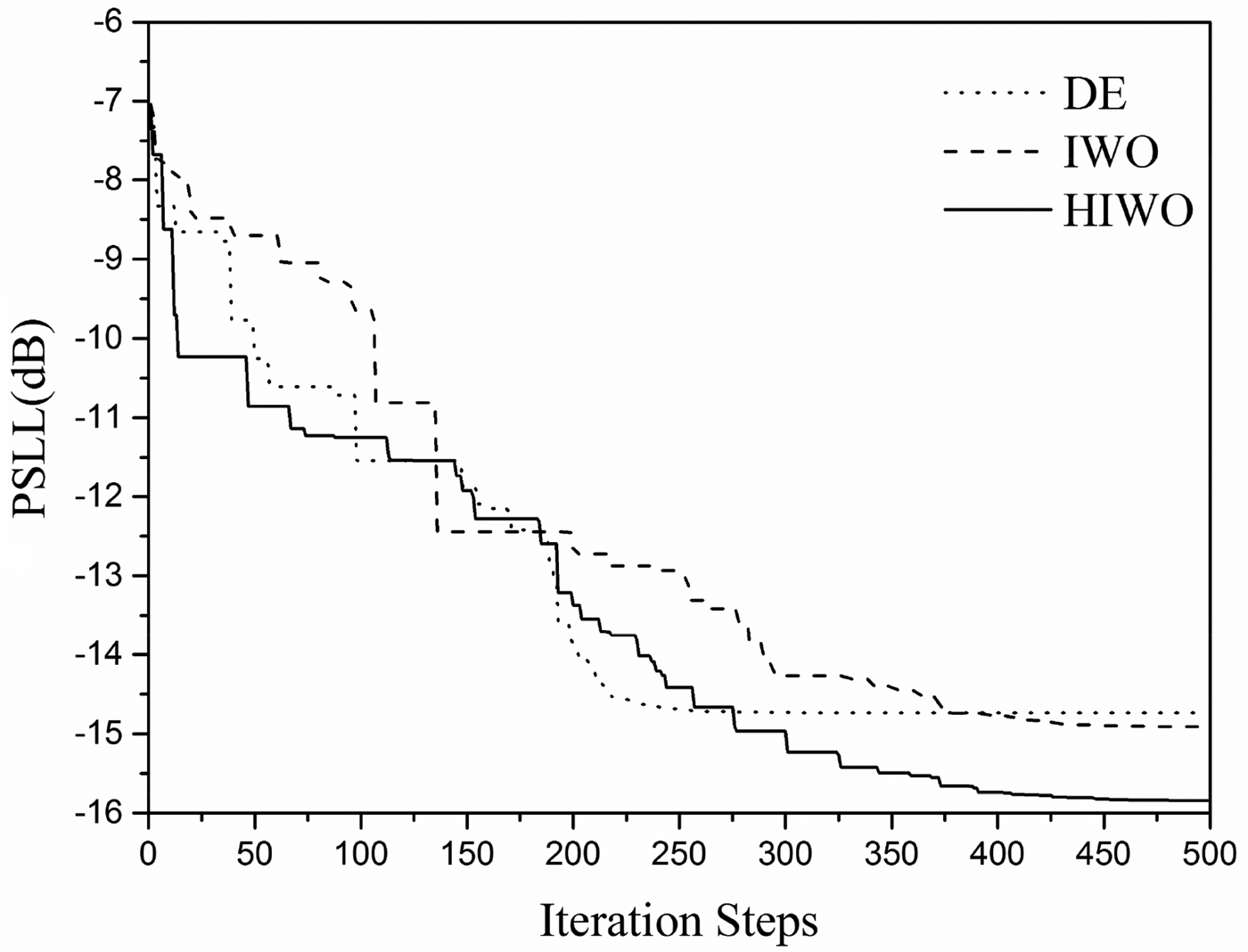
For the first synthesis example, the circular antenna array with eight elements is optimized. The same array is synthesized in [Reference Singh and Kamal9] using BBO. The length of the antenna array is L = 9.0717λ. So, the radius of the circular antenna array is R = L/2π. The minimum angular spacing of the adjacent elements is φe = 19.84o. Compared with the result optimized in [Reference Singh and Kamal9], in order to obtain the radiation pattern with approximate beamwidth, the desired FNBW is 42o. Table 2 gives the excitation amplitudes and angular positions of the array elements synthesized by BBO, DE, IWO, and HIWO. It can be seen from Table 2 that HIWO can obtain the best PSLL which is lower by 1.34, 1.19, and 0.32 dB than those calculated by BBO, DE, and IWO. The FNBW and 3 dB beamwidth (3 dB BW) of the radiation pattern synthesized by HIWO are 41.47o and 17.42o, respectively. The optimized angular positions of the array elements also fulfil the minimum spacing constraint. The convergence curve of DE, IWO, and HIWO is given in Fig. 3. The radiation patterns optimized by BBO, DE, IWO, and HIWO are given in Fig. 4.
Synthesis results obtained by BBO [Reference Singh and Kamal9], DE, IWO and HIWO (8-element circular antenna array).

PSLL versus iteration steps (8-element circular antenna array).

Radiation pattern synthesized by BBO [Reference Singh and Kamal9], DE, IWO, and HIWO (8-element circular antenna array).

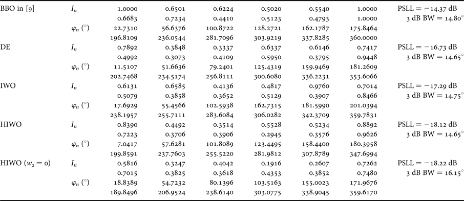
If the beamwidth of the radiation pattern is not constrained which can be fulfilled by setting w 2 = 0 in (4), the PSLL of the synthesized radiation pattern is −13.96 dB. The FNBW and 3 db BW are 50.58o and 19.88o, respectively. The radiation pattern is given in Fig. 4. The excitation amplitudes and angular positions of the elements are given in Table 2.
B) Optimization result of 10-element circular antenna array
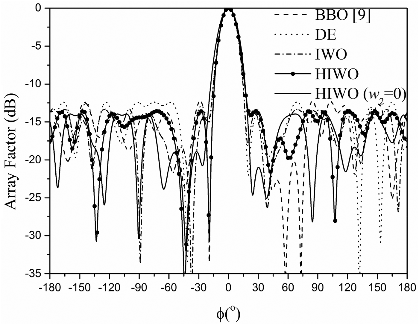
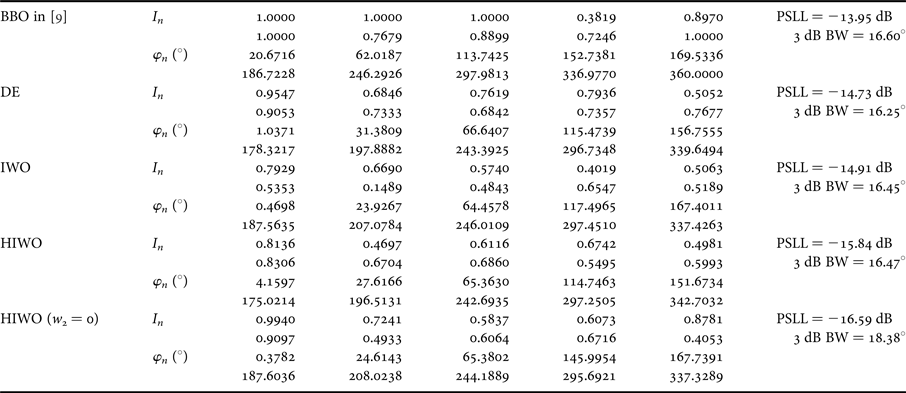
In this example, the synthesis result of 10-element circular antenna array is given. The length of the antenna array is L = 9.2318λ. So, the minimum angular spacing of the adjacent elements is φe = 19.49o. The desired FNBW is 40o. In Table 3, the excitation amplitudes and angular positions of the array elements synthesized by BBO, DE, IWO, and HIWO are given. It can be seen from Table 3 that HIWO can obtain the best PSLL which is lower by 1.89, 1.11, and 0.93 dB than those calculated by BBO, DE, and IWO. The FNBW and 3 dB BW of the radiation pattern synthesized by HIWO are 38.45o and 16.47o. The minimum calculated angular spacing of the adjacent array element is 21.45o which fulfil the minimum spacing constraint. The convergence curve of DE, IWO, and HIWO is given in Fig. 5. The radiation patterns optimized by BBO, DE, IWO, and HIWO are given in Fig. 6.
Synthesis results obtained by BBO [Reference Singh and Kamal9], DE, IWO, and HIWO (10-element circular antenna array).

PSLL versus iteration steps (10-element circular antenna array).

Radiation pattern synthesized by BBO [Reference Singh and Kamal9], DE, IWO, and HIWO (10-element circular antenna array).

When the beamwidth of the radiation pattern is not constrained, the PSLL of the synthesized radiation pattern is −16.59 dB. The FNBW and 3 db BW are 43.80o and 18.38o. The radiation pattern is given in Fig. 6. The excitation amplitudes and angular positions of the elements are provided in Table 3.
C) Optimization result of 12-element circular antenna array
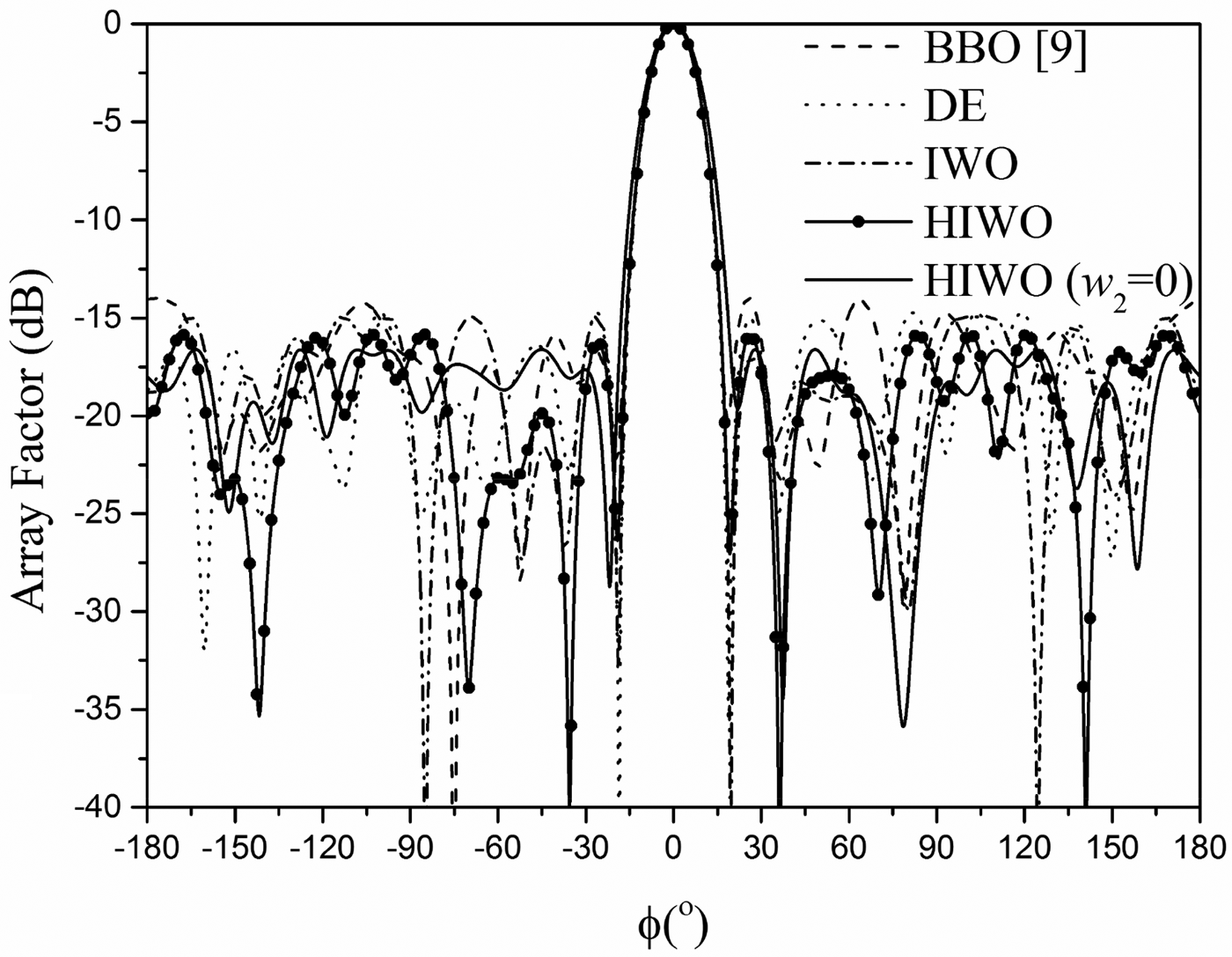
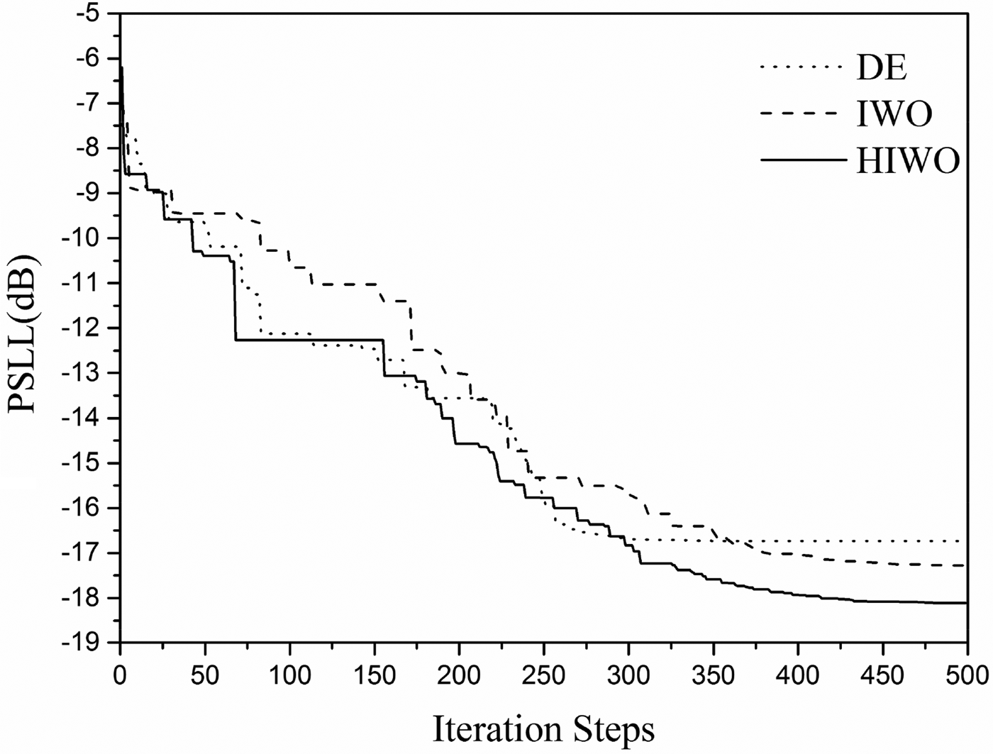
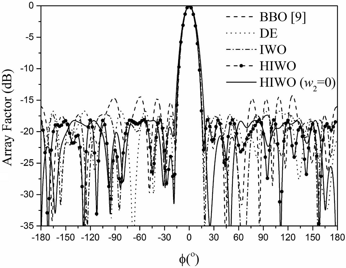
For the last example, synthesis of 12-element circular antenna array is introduced. The length of the antenna array is L = 10.6174λ and the minimum angular spacing of the adjacent elements is φe = 16.95o. The desired FNBW is chosen to be 36o. The excitation amplitudes and angular positions of the array elements synthesized by BBO, DE, IWO, and HIWO are given in Table 4. It can be seen that HIWO can obtain the best PSLL which is 3.748, 1.39, and 0.83 dB lower than those obtained by BBO, DE, and IWO, respectively. The FNBW and 3 dB BW of the radiation pattern synthesized by HIWO are 36.0o and 14.65o. The minimum angular spacing of the adjacent array element calculated by HIWO is 17.76o which fulfil the minimum spacing constraint. The convergence curve of IWO and HIWO is given in Fig. 7. The radiation patterns optimized by BBO, IWO, and HIWO are given in Fig. 8.
Synthesis results obtained by BBO [Reference Singh and Kamal9], DE, IWO, and HIWO (12-element circular antenna array).

PSLL versus iteration steps (12-element circular antenna array).

Radiation pattern synthesized by BBO [Reference Singh and Kamal9], DE, IWO, and HIWO (12-element circular antenna array).

The PSLL, FNBW, and 3 db BW of the synthesized radiation pattern are −18.22 dB, 44.80o and 16.15o when the beamwidth of the radiation pattern is not constrained. Figure 8 shows the radiation pattern. The excitation amplitudes and angular positions of the array elements are provided in Table 4.
V. CONCLUSION
A new synthesis method of non-uniform circular antenna arrays is introduced in this paper. For the first time, the method proposed in this paper can constrain the number of array elements, size of the antenna array, and minimum spacing of the adjacent elements simultaneously. The excitation amplitudes and angular position of the array elements are optimized by HIWO. Compared with BBO, DE, and IWO, the radiation pattern synthesized by HIWO can obtain much lower PSLL. Synthesis results reveal that the design method of this non-uniform circular antenna arrays provides a considerable side lobe level reduction.
ACKNOWLEDGEMENT
This work was supported by Natural Science Foundation of Shaanxi Provincial Department of Education under grant No. 17JK0319 and by Doctoral Scientific Research Foundation of Xi'an Polytechnic University under grant No. 107020277 and No. BS1413.
 Hua Guo received his Ph.D. degree in Electromagnetic Fields and Microwave Techniques from Northwestern Polytechnical University. He is now a lecturer of Signal and Information Processing in Xi'an Polytechnic University. His research interests include electromagnetic theory and calculation, array antenna design, phased arrays, and radars.
 Lin Cui received her Ph.D. degree in Acoustics from Northwestern Polytechnical University in 2013. Since 2013, she has been a lecturer of Signal and Information Processing in Xi'an Polytechnic University. Her research interests include underwater acoustic signal processing, optimization of array beamforming, and signal detection.
 Xiaodan Zhang received her Ph.D. degree in Information and Communication Engineering from Xi'an University of Technology in 2012. She is now a lecturer of Signal and Information Processing in Xi'an Polytechnic University. Her research interests include image processing and imaging of wave signals.
 Yameng Jiao received her Ph.D. degree in Information and Communication Engineering from Northwestern Polytechnical University in 2013. She is now a lecturer of Signal and Information Processing in Xi'an Polytechnic University. Her research interests include array signal processing and intelligent algorithms.