1 Introduction
Turbulent thermal convection plays very important role in a range of phenomena in astrophysical and geophysical systems, where the underlying surfaces over which convective turbulence occurs are always rough. As an idealised model for the study of turbulent thermal convection in general, turbulent Rayleigh–Bénard convection (RBC), where a fluid layer confined between two horizontally parallel plates heated from below and cooled from above, has been studied extensively in the past two decades (for reviews, see e.g. Siggia Reference Siggia1994; Ahlers, Grossmann & Lohse Reference Ahlers, Grossmann and Lohse2009; Lohse & Xia Reference Lohse and Xia2010; Chillá & Schumacher Reference Chillá and Schumacher2012; Xia Reference Xia2013). In terms of equations of motion, there are two control parameters in RBC, i.e. the Rayleigh number
 $Ra=\unicode[STIX]{x1D6FC}g\unicode[STIX]{x0394}TH^{3}/(\unicode[STIX]{x1D708}\unicode[STIX]{x1D705})$
and the Prandtl number
 $Pr=\unicode[STIX]{x1D708}/\unicode[STIX]{x1D705}$
, where
 $\unicode[STIX]{x0394}T$
is the applied temperature difference across a fluid layer of height
 $H$
,
 $g$
is the gravitational acceleration constant and
 $\unicode[STIX]{x1D6FC}$
,
 $\unicode[STIX]{x1D705}$
and
 $\unicode[STIX]{x1D708}$
are respectively the thermal expansion coefficient, the thermal diffusivity and the kinematic viscosity of the working fluid. Any laboratory convection experiments are confined, thus the aspect ratio
 $\unicode[STIX]{x1D6E4}$
and the container shape come into the problem.
One of the central issues in the study of turbulent RBC is to determine how the response parameters, i.e. the Nusselt number
 $Nu$
and the Reynolds number
 $Re$
, depend on the control parameters, where
 $Nu$
is a measurement of the system’s heat transport efficiency and
 $Re$
quantifies the turbulence intensity. The functional forms of
 $Nu(Ra,Pr)$
and
 $Re(Ra,Pr)$
are usually expressed in terms of power laws:
 $$\begin{eqnarray}Nu\sim Ra^{\unicode[STIX]{x1D6FC}}Pr^{\unicode[STIX]{x1D701}},\quad Re\sim Ra^{\unicode[STIX]{x1D6FD}}Pr^{\unicode[STIX]{x1D716}}.\end{eqnarray}$$
A comprehensive review on this issue can be found in Ahlers et al. (Reference Ahlers, Grossmann and Lohse2009). It is now generally accepted that there are multiple scalings in the
 $Ra$
–
 $Pr$
phase space where the bulk flow is in a turbulent state according to the Grossmann and Lohse model for turbulent thermal convection in a convection cell with smooth surface (Grossmann & Lohse Reference Grossmann and Lohse2000, Reference Grossmann and Lohse2001, Reference Grossmann and Lohse2002, Reference Grossmann and Lohse2004).
Compared with the large number of studies of turbulent convection in convection cells with smooth plates, studies of turbulent convection in cells with rough plates are relatively scarce. However, in addition to its fundamental importance in geophysical and astrophysical problems, turbulent thermal convection over rough surfaces is found to be a more effective way to transport heat, which is also useful in practical applications. The enhancement of heat transport is first observed when the top and bottom plates are rough and the thermal boundary layer (BL) is thinner than the roughness height (Shen, Tong & Xia Reference Shen, Tong and Xia1996). The enhancement is later found to be due to more thermal plumes being emitted from the tip of the roughness elements (Du, Tong & Xia Reference Du, Tong and Xia1998).
Although the heat transport is enhanced, the scaling relation between
 $Nu$
and
 $Ra$
is found to be insensitive to the plate morphology (Shen et al.
Reference Shen, Tong and Xia1996; Du et al.
Reference Du, Tong and Xia1998). Several later experiments show that the scaling exponents can also change in convection cells with rough plates (rough cells hereafter) when compared with observations in convection cells with smooth plates (smooth cells hereafter). Using glass spheres adhered to the bottom plate of the convection cell, the scaling exponent is found to depend on the distribution of the roughness height (Ciliberto & Laroche Reference Ciliberto and Laroche1999). For
 $Ra>10^{12}$
, a scaling exponent of
 $0.5$
is reported when grooved roughness is distributed on both the plates and side wall of the convection cell (Roche et al.
Reference Roche, Castaing, Chabaud and Hébral2001). A change of the scaling exponent from 0.28 in a smooth cell to 0.35 in a rough cell is observed (Qiu, Xia & Tong Reference Qiu, Xia and Tong2005). Although the rough cell used in the experiments of (Qiu et al.
Reference Qiu, Xia and Tong2005) had similar design to the ones used in Shen et al. (Reference Shen, Tong and Xia1996) and Du et al. (Reference Du, Tong and Xia1998), different scaling exponents
 $\unicode[STIX]{x1D6FC}$
were observed. Qiu et al. (Reference Qiu, Xia and Tong2005) have suggested that the discrepancy between their experiments and those of Shen et al. (Reference Shen, Tong and Xia1996) and Du et al. (Reference Du, Tong and Xia1998) may be attributed to the different constructions and materials of the rough plates. In the earlier experiments, rough plates made of brass were attached on the surfaces the top and bottom smooth plates while in the later experiment, the roughness elements were directly machined on a piece of copper.
In addition to studying the global transport properties of the convection cell, the heat transport properties of individual plates with rough/smooth surfaces were also investigated (Wei et al.
Reference Wei, Chan, Ni, Zhao and Xia2014). It is found that heat transport property of individual plate differs significantly and depends on the nature of the opposite plate of the same convection cell and the pertaining temperature boundary conditions. By determining the
 $Nu$
separately for the bottom rough plate and the top smooth plate, a scaling exponent of
 $1/2$
for the rough plate and of
 $1/3$
for the smooth plate are reported (Tisserand et al.
Reference Tisserand, Creyssels, Gasteuil, Pabiou, Gibert, Castaing and Chillá2011).
The effects of roughness elements on the local dynamics of turbulent RBC are also studied. Using flow visualisation and near-wall temperature measurements, it is shown that the interaction of the large-scale circulation (LSC) and the secondary flow in the grooved region of the rough plate enhances plume emission which leads to the enhancement of heat transport (Du & Tong Reference Du and Tong2000). Consistent with this picture, the study of local temperature fluctuations suggests that the enhancement of heat transport is determined by the dynamics in the near-plate region (Du & Tong Reference Du and Tong2001). The effects of rough plates on the velocity BL have been investigated very recently (Liot et al. Reference Liot, Salort, Kaiser, du Puits and Chillá2016), where it is found that the flow field is very different before and after the heat transport enhancement transition.
Direct numerical simulation (DNS) of turbulent RBC in rough cells also shows that the scaling exponent increases (Stringano, Pascazio & Verzicco Reference Stringano, Pascazio and Verzicco2006; Shishkina & Wagner Reference Shishkina and Wagner2011; Toppaladoddi, Succi & Wettlaufer Reference Toppaladoddi, Succi and Wettlaufer2015; Wagner & Shishkina Reference Wagner and Shishkina2015; Toppaladoddi, Succi & Wettlaufer Reference Toppaladoddi, Succi and Wettlaufer2017). The scaling exponent
 $\unicode[STIX]{x1D6FC}$
increases from 0.31 in a smooth cell to 0.37 in a cylindrical rough cell with grooved walls at the top and bottom plates (Stringano et al.
Reference Stringano, Pascazio and Verzicco2006). In addition, this scaling exponent was also found to depend on the geometry of the roughness elements or ‘obstacles’ in a quasi-two-dimensional DNS (Wagner & Shishkina Reference Wagner and Shishkina2015). But the number of roughness elements in this study is very limited (only 4 ‘obstacles’ were used). In a two-dimensional (2-D) study, using sinusoidal rough elements, the scaling exponent
 $\unicode[STIX]{x1D6FC}$
is also found to depend on the wavelength of the roughness elements (Toppaladoddi et al.
Reference Toppaladoddi, Succi and Wettlaufer2015, Reference Toppaladoddi, Succi and Wettlaufer2017). In a DNS study of turbulent Taylor–Couette flow the scaling exponent was also found to increase with wall roughness (Zhu et al.
Reference Zhu, Ostilla-Mónico, Verzicco and Lohse2016). These numerical studies highlight the importance of roughness geometry on turbulent transport. However, the limited number of roughness element in a 3-D or a (quasi-) 2-D computation domain makes the comparison between the DNS studies and experimental ones less straightforward.
On the experimental side, although there are quite a number of studies focusing on the effects of roughness on turbulent RBC, to the best of our knowledge no experimental investigations have been made to systematically vary roughness geometry. This motivates the present study in which the effects of varying roughness geometry on turbulent RBC have been investigated systematically. A parameter
 $\unicode[STIX]{x1D706}$
, which is defined as the height of a single roughness element over its base width, is used to characterise the geometry of the roughness elements. In addition to the heat transport enhancement as found by previous studies, we show that the heat transport scaling in a rough cell with fixed roughness height
 $h$
may be classified into three regimes. The experiments further demonstrate that
 $\unicode[STIX]{x1D706}$
can be used as a tuning parameter to manipulate heat transport scaling in rough cells in the heat transport enhanced regime. The Reynolds number and local temperature fluctuation scalings with
 $Ra$
also change with
 $\unicode[STIX]{x1D706}$
, suggesting that the geometry of roughness elements not only alters the global heat transport of the system but also influences the bulk turbulence and the dynamics of the LSC.
The remainder of the paper is organised as follows: the experimental set-up and measurement techniques are introduced in § 2, which is divided into four subsections. The construction of the convection cell is described in § 2.1. The properties of the working fluids used and the explored
 $Ra$
–
 $Pr$
–
 $\unicode[STIX]{x1D706}$
phase space are introduced in § 2.2. The temperature measurement techniques are documented in § 2.3 and § 2.4 introduces the measurement of the viscous BL using particle image velocimetry (PIV). Section 3 presents the experimental findings. The effects of roughness geometry on the heat transport are reported in § 3.1. The transitions between different heat transport regimes are discussed in § 3.2. The Reynolds number and local temperature fluctuation measurements are presented in §§ 3.3 and 3.4, respectively. A discussion of the proper parameter that characterises the system is reported in § 3.5. We summarise and conclude our findings in § 4.
2 Experimental set-up and measurement techniques
2.1 The convection cell
The experiments were carried out in four cylindrical convection cells. Each of the convection cells consisted of top and bottom plates and a Plexiglas side wall. Except for the geometry of roughness elements on the top and bottom plates, the constructions of the convection cells were otherwise identical.
The side wall was made of Plexiglas tube with a wall thickness of 4 mm. The convection cells had a diameter
 $D$
of 19.2 cm and a height
 $H$
of 20.3 cm measured from the base of the roughness elements. Thus the aspect ratios
 $\unicode[STIX]{x1D6E4}=D/H$
of the convection cells were approximately unity. The top and bottom plates were made of 12 mm thick copper except for the ones for rough cells with
 $\unicode[STIX]{x1D706}=1.9$
which were made of aluminium. The thermal conductivity of aluminium is
 $205~\text{W}~{\text{m}^{-1}\,}^{\circ }\text{C}^{-1}$
at temperature
 $25\,^{\circ }\text{C}$
, which is approximately half that of copper. The differences in heat transport properties in convection cells with plates made of copper and aluminium, i.e. the effects of the finite conductivity of the plates (Verzicco Reference Verzicco2004; Brown et al.
Reference Brown, Nikolaenko, Funfschilling and Ahlers2005), have been shown to be minimal in the
 $Ra$
and
 $Pr$
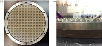
range reported in the present studies (Wei, Ni & Xia Reference Wei, Ni and Xia2012). The pyramid-shaped roughness elements were directly machined on the top and bottom plates that were then plated with nickel to prevent oxidation. The roughness elements were arranged in a square lattice form (see figure 1), which was the same as those used previously (Wei et al.
Reference Wei, Chan, Ni, Zhao and Xia2014; Xie et al.
Reference Xie, Huang, Funfschilling, Li, Ni and Xia2015). By keeping the height of roughness elements
 $h$
a constant at 8 mm and changing the base width
 $w$
of individual roughness elements from 16 mm to 2 mm, rough plates with roughness parameter
 $\unicode[STIX]{x1D706}$
, defined as the ratio of
 $h$
and
 $w$
, at 0.5, 1.0, 1.9 and 4.0 were used in the present study. With the increase of
 $\unicode[STIX]{x1D706}$
, the number density
 $n$
(in unit of number of roughness element per
 $\text{cm}^{2}$
) also increases, i.e.
 $n=0.38$
(
 $\unicode[STIX]{x1D706}=0.5$
),
 $1.5~(\unicode[STIX]{x1D706}=1.0)$
, 6.1 (
 $\unicode[STIX]{x1D706}=1.9$
) and 24.5 (
 $\unicode[STIX]{x1D706}=4.0$
). To clarify whether the number density or the
 $\unicode[STIX]{x1D706}$
is the key parameter that characterises the system, another set of rough plates with
 $\unicode[STIX]{x1D706}=4.0$
and a roughness height of 4 mm was used (
 $n$
was increased by a factor of 4 in this case). The present study implies that
 $\unicode[STIX]{x1D706}$
is a more suitable parameter to characterise the geometry of the roughness elements and the response of the system, rather than the number density of the roughness elements.
The top plate was cooled by passing temperature-controlled water from a water circulating bath through a chamber fitted on its top (Poly Science, 9702). The cooling water entered the chamber through two inlets and left the chamber through two outlets. The arrangements of the inlets and outlets were such that the two inlets were along one diameter of the plate and the two outlets were along another diameter perpendicular to the inlets. Temperature stability of the cooling water was better than
 $0.01\,^{\circ }\text{C}$
. Furthermore, a stirring blade driven by the inlet and outlet flows was installed inside the cooling chamber to ensure temperature uniformity across the top plate. The bottom plate was electrically heated by two rubber heaters connected in series and sandwiched in between the bottom plate and a copper plate with a thickness of 10 mm (see, e.g. figure 1). The heaters were connected to a DC power supply with a long term voltage stability of 99.99 % (Sorensen, XFR300-4). To ensure good thermal contact, a thin layer of thermally conductive paste was used between the heaters and the plates. The largest temperature difference within the same plate was approximately
 $1.5\,\%\unicode[STIX]{x0394}T$
. It should be noted that in this arrangement, the temperature boundary condition for the top plate was constant temperature and that for the bottom plate was constant heat flux.
To prevent heat leakage and to minimise the influence of the environmental temperature fluctuation, the convection cells were wrapped with Styrofoam with a thickness of 6 cm. A temperature regulated copper basin was placed beneath the convection cell to prevent heat leakage from the bottom plate by maintaining the same temperature at the top and bottom of the basin. The whole set-up was put into a thermostat where the temperature was regulated to match the mean temperature
 $T_{m}$
of the top and bottom plates. The temperature stability of the thermostat was better than
 $0.1\,^{\circ }\text{C}$
.
Photos of the bottom plate of a rough cell with
 $\unicode[STIX]{x1D706}=1.0$
. (a) Top view; (b) side view. The red heater connection wires can be seen at the top of (a). Plates with
 $\unicode[STIX]{x1D706}$
values of 0.5, 1.9 and 4.0 have the same design.

2.2 The working fluids
Only approximately one and a half decades of
 $Ra$
can be achieved in a single experimental set-up using a classical working fluid such as water. To extend the
 $Ra$
range, two kinds of working fluids, namely deionised water and Flourinert FC770 (FC770 hereafter, 3M Inc.) were used. Water has been widely used in the study of turbulent convection and we will mention here only the properties of FC770. The data listed below are given by the manufacturer (3M Inc.) and are all obtained at the temperature
 $25~^{\circ }\text{C}$
. The FC770 has
 $\unicode[STIX]{x1D712}=0.063~\text{W}~{\text{m}^{-1}~}^{\circ }\text{C}^{-1}$
,
 $\unicode[STIX]{x1D6FC}=0.00148~^{\circ }\text{C}$
,
 $\unicode[STIX]{x1D708}=7.9\times 10^{-7}~\text{m}^{2}~\text{s}^{-1}$
, the specific heat
 $c_{p}=1038~\text{J}~{\text{kg}^{-1}~}^{\circ }\text{C}^{-1}$
and the density
 $\unicode[STIX]{x1D70C}=1793~\text{kg}~\text{m}^{-3}$
.
The working fluid was filled into the convection cell through a hole attached with a stainless steel tube (
 ${\sim}8$
mm in diameter) located at the centre of the top plate. The working fluids were degassed in the following way to ensure there was no bubble forming during a single run of the experiment (i.e. a
 $Ra$
scan of
 $Nu$
for a fixed
 $Pr$
), which typically lasted for three weeks. Deionised water was boiled for a hour and then cooled down to room temperature before filling into the convection cell. For FC770, it was first filled into the convection cell and degassed by keeping the temperature of the top and bottom plate, and thus the whole convection cell, at
 $50\,^{\circ }\text{C}$
for 24 h. Then the temperature of the convection cell was then lowed to
 $25\,^{\circ }\text{C}$
which was the
 $T_{m}$
for all the experiments using FC770, and the bubbles formed were totally removed.
 $Ra$
–
 $Pr$
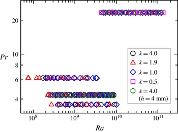
phase space explored for different values of
 $\unicode[STIX]{x1D706}$
. The case for
 $\unicode[STIX]{x1D706}=0.5$
is only studied for
 $Pr=23.34$
. All experiments were conducted in convection cells with roughness height
 $h=8$
mm, except for the ones corresponding to hexagons that were conducted in convection cell with
 $h=4~\text{mm}$
.

The explored
 $Ra$
and
 $Pr$
phase space at different values of
 $\unicode[STIX]{x1D706}$
is shown in figure 2. Except for
 $\unicode[STIX]{x1D706}=0.5$
which was investigated for a single
 $Pr$
(23.34) in the present studies, all the other values of
 $\unicode[STIX]{x1D706}$
were studied for the four values of
 $Pr$
, i.e.
 $Pr=3.67$
(water,
 $T_{m}=50.0\,^{\circ }\text{C}$
),
 $Pr=4.34$
(water,
 $T_{m}=40.0\,^{\circ }\text{C}$
),
 $Pr=6$
.14 (water,
 $T_{m}=25.0\,^{\circ }\text{C}$
) and
 $Pr=23.34$
(FC770,
 $T_{m}=25.0\,^{\circ }\text{C}$
). The experiments covered
 $7.50\times 10^{7}\leqslant Ra\leqslant 1.31\times 10^{11}$
. The temperature differences applied across the convection cell using water as the working fluid for different values of
 $\unicode[STIX]{x1D706}$
were:
 $0.98\,^{\circ }\text{C}$
to
 $26.99\,^{\circ }\text{C}$
(
 $\unicode[STIX]{x1D706}=4.0$
);
 $0.47\,^{\circ }\text{C}$
to
 $20.16\,^{\circ }\text{C}$
(
 $\unicode[STIX]{x1D706}=1.9$
) and
 $0.89\,^{\circ }\text{C}$
to
 $24.75\,^{\circ }\text{C}$
(
 $\unicode[STIX]{x1D706}=1.0$
). The temperature differences applied using FC770 as working fluid at different values of
 $\unicode[STIX]{x1D706}$
were:
 $1.40\,^{\circ }\text{C}$
to
 $22.14\,^{\circ }\text{C}$
(
 $\unicode[STIX]{x1D706}=4.0$
);
 $0.99\,^{\circ }\text{C}$
to
 $17.25\,^{\circ }\text{C}$
(
 $\unicode[STIX]{x1D706}=1.9$
);
 $1.11\,^{\circ }\text{C}$
to
 $27.63\,^{\circ }\text{C}$
(
 $\unicode[STIX]{x1D706}=1.0$
) and
 $0.96\,^{\circ }\text{C}$
to
 $29.66\,^{\circ }\text{C}$
(
 $\unicode[STIX]{x1D706}=0.5$
).
2.3 The temperature measurements
Temperature of the top plate was measured using four thermistors (Omega, Model 44031) embedded at a distance of
 $D/4$
from the centre of the plate and uniformly in the azimuthal direction. Four thermistors at the mirror location of the top plate embedded in the bottom plate with one additional thermistor at the centre of it were used to measure the temperature of the bottom plate. The thermistors were calibrated individually and separately in a temperature-controlled water bath. The temperature range of calibration was from
 $5\,^{\circ }\text{C}$
to
 $70\,^{\circ }\text{C}$
with a temperature accuracy better than
 $0.01\,^{\circ }\text{C}$
. The resistances of the thermistors were measured using a
 $6(1/2)$
digital multimeter (Keithley, 2700) and were converted to temperature using the calibration curve. The sampling rate of the temperature measurement was
 ${\sim}0.7$
Hz.
Local temperatures at the cell centre and
 ${\sim}1~\text{cm}$
away from the side wall were measured using two small thermistors with a bead diameter of
 $0.38~\text{mm}$
and a time constant of 30 ms in liquid (Measurement Specialities, Model: G22K7MCD419). These small thermistors had a temperature accuracy of
 $0.01\,^{\circ }\text{C}$
. They were guided into the convection cell using a stainless steel tube with an outer diameter of 1.1 mm and wall thickness of 0.2 mm (Goodfellow, Stainless Steel – AISI 304 Tube). Each of the small thermistors had an independent temperature measurement system specially designed to measure the temperature fluctuation. Detailed design of the measurement system can be found in Zhou & Xia (Reference Zhou and Xia2001). Briefly, the thermistor acted as one arm of a AC Wheatstone electrical bridge. The resistance fluctuations of the thermistor induced by the temperature fluctuations in the convection cell were converted to the voltage fluctuations of the electrical bridge which were magnified using a lock-in amplifier (Stanford Research System, SR830). The output signal from the lock-in amplifier was then digitised and stored by a dynamic signal analyser (HP, 35670A). The measured voltage was converted to resistance and then to temperature using the calibration curve of the thermistors. The sampling rate of the local temperature varied from 16 Hz to 128 Hz depending on
 $Ra$
and
 $Pr$
to ensure that the small-scale temporal temperature fluctuations were fully resolved.
From the temperature measurements, the heat transport across the convection cell, i.e. the Nusselt number
 $Nu=qH/(\unicode[STIX]{x1D712}\unicode[STIX]{x0394}T\unicode[STIX]{x03C0}(D/2)^{2})$
, local temperatures and the Reynolds number
 $Re=UH/\unicode[STIX]{x1D708}$
were measured as a function of
 $Ra$
,
 $Pr$
and
 $\unicode[STIX]{x1D706}$
, where
 $q$
was the input heating power at the bottom plate,
 $\unicode[STIX]{x1D712}$
was the thermal conductivity of the working fluid and
 $U$
was the characteristic velocity of the LSC. Each measurement lasted at least 12 h after the system had reached a steady state to ensure that the system had explored all flow states.
2.4 The viscous boundary layer measurements
The dynamics of the viscous boundary layer in the rough cell with
 $\unicode[STIX]{x1D706}=1.0$
was measured using a commercial PIV system that had been documented elsewhere (Xia, Sun & Zhou Reference Xia, Sun and Zhou2003). The flow was seeded with particles with a diameter of
 $2~\unicode[STIX]{x03BC}\text{m}$
and density matched with water. A 2-D flow region with a size of
 $20~\text{mm}\times 28~\text{mm}$
was measured within the LSC’s circulation plane with
 $x$
denoting the direction along the circulation path of the LSC and
 $z$
denoting the direction pointing upwards at the centre of bottom plate (see, e.g. figure 7). The origin of the coordinate system was located at the centre of the plate. To minimise optical distortion of the particle images induced by the curved surface of the cell, a jacket filled with water with flat window was adhered to the convection cell. The optical arrangement was such that the measurement plane was within one groove of the rough plate and the images were acquired perpendicular to it. A mask with the shape exactly matching that of the plate geometry was applied to the captured images to exclude the parts blocked by the roughness elements.
The velocity field was obtained by cross-correlating two consecutive images taken with a time separation that matched the velocity of the flow at different
 $Ra$
. The velocity map consisted of
 $63\times 79$
vectors in the
 $x$
- and
 $z$
- directions respectively. Totally 26 136 vector maps were acquired at a sampling rate of 2.2 Hz, which lasted for
 ${\sim}3.3$
h. The velocity fluctuation map was obtained by subtracting the mean velocity map from each of the instantaneous velocity map. The measurements were done at
 $Pr=4.34$
and
 $3.55\times 10^{8}\leqslant Ra\leqslant 9.62\times 10^{9}$
. To lock the direction of the LSC, the convection cell was tilted with respect to the vertical direction by
 ${\sim}0.5^{\circ }$
.
3 Results and discussion
3.1 Heat transport measurements
We show in this section that the heat transport in turbulent RBC over rough plates may be classified into three regimes based on the scaling law of
 $Nu$
versus
 $Ra$
. In addition, the heat transport scaling in the enhanced regime (Regimes II and III) can be manipulated by changing the roughness geometry. The transition from Regime I to Regime II in a rough cell with
 $h=4$
mm and
 $\unicode[STIX]{x1D706}=4.0$
is discussed in section § 3.1.1. The heat transport measurement with changing the geometry of roughness elements, i.e. for different values of
 $\unicode[STIX]{x1D706}$
, is presented in § 3.1.2 together with the observation of Regime II and Regime III.
3.1.1 Transition from Regime I to Regime II
Previously, Shen et al. (Reference Shen, Tong and Xia1996) found that the heat transport cannot be altered in a rough cell if the thermal BL thickness
 $\unicode[STIX]{x1D6FF}_{th}$
is larger than the height of the roughness elements. We call this Regime I of convective turbulence in a rough cell. As
 $\unicode[STIX]{x1D6FF}_{th}$
decreases with increasing
 $Ra$
, it will eventually become smaller than the roughness height, i.e.
 $\unicode[STIX]{x1D6FF}_{th}<h$
. When this happens turbulent convection enters a new, the heat transport enhanced regime, termed Regime II here. This regime has been observed by a number of previous experiments (Shen et al.
Reference Shen, Tong and Xia1996; Du et al.
Reference Du, Tong and Xia1998; Qiu et al.
Reference Qiu, Xia and Tong2005; Tisserand et al.
Reference Tisserand, Creyssels, Gasteuil, Pabiou, Gibert, Castaing and Chillá2011; Wei et al.
Reference Wei, Chan, Ni, Zhao and Xia2014).
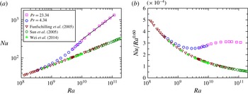
We plot in figure 3(a)
 $Nu$
as a function of
 $Ra$
in a rough cells with
 $h=4~\text{mm}$
and
 $\unicode[STIX]{x1D706}=4.0$
. For comparison, the data from Funfschilling et al. (Reference Funfschilling, Brown, Nikolaenko and Ahlers2005) in a smooth cell with
 $\unicode[STIX]{x1D6E4}=1,Pr=4.38$
, from Wei et al. (Reference Wei, Chan, Ni, Zhao and Xia2014) in a smooth cell with
 $\unicode[STIX]{x1D6E4}=1,Pr=4.34$
and from Sun et al. (Reference Sun, Ren, Song and Xia2005) in a smooth cell with
 $\unicode[STIX]{x1D6E4}=2,Pr=4.34$
are plotted respectively as down-pointing triangles, hexagons and stars. Figure 3(b) plots the corresponding data in a compensated form. It is seen that
 $Nu$
in the rough cell first overlaps nicely with those from the smooth cells for
 $Ra<4\times 10^{8}$
. With increasing
 $Ra$
, there is a gradual transition, where the heat transport enhances. Within the transitional
 $Ra$
range
 $4\times 10^{8}<Ra<1\times 10^{10}$
, there is no well-defined scaling law between
 $Nu$
and
 $Ra$
. For
 $Ra>1\times 10^{10}$
, the data show a power-law relation, i.e.
 $Nu\sim Ra^{0.60}$
. These data clearly demonstrate the transition from Regime I to Regime II. Such a transition is also observed by Wei et al. (Reference Wei, Chan, Ni, Zhao and Xia2014) in a rough cell with
 $h=3~\text{mm}$
. Using the relation
 $\unicode[STIX]{x1D6FF}_{th}=H/(2Nu)$
(which was valid only for the plate-wise averaged thermal BL thickness and for a smooth cell), we had
 $\unicode[STIX]{x1D6FF}_{th}=2.1~\text{mm}$
at
 $Ra=3.4\times 10^{8}$
, which might be considered to be close to the roughness height of 4 mm in an order of magnitude sense and broadly consistent with the proposed interpretation by Shen et al. (Reference Shen, Tong and Xia1996).
3.1.2 Effects of roughness geometry in the heat transport enhanced regime
We present measurements of
 $Nu$
as a function of
 $Ra$
in convection cells with a roughness height
 $h$
of 8 mm and different roughness geometries in this subsection. The roughness height was much larger than
 $\unicode[STIX]{x1D6FF}_{th}$
for the explored range of
 $Ra$
. Therefore, Regime I behaviour was not observed here. Instead, we focus on Regime II and Regime III (a new regime to be defined below).
(a)
 $Nu$
as a function of
 $Ra$
in a rough cell with a roughness elements height of 4 mm. The down-pointing triangles are taken from Funfschilling et al. (Reference Funfschilling, Brown, Nikolaenko and Ahlers2005) (
 $\unicode[STIX]{x1D6E4}=1.0,Pr=4.38$
), the hexagons are taken from Sun et al. (Reference Sun, Ren, Song and Xia2005) (
 $\unicode[STIX]{x1D6E4}=2.0,Pr=4.34$
), the stars are taken from Wei et al. (Reference Wei, Chan, Ni, Zhao and Xia2014) (
 $\unicode[STIX]{x1D6E4}=1.0,Pr=4.34$
). (b) The compensated plot of the same data as in (a).

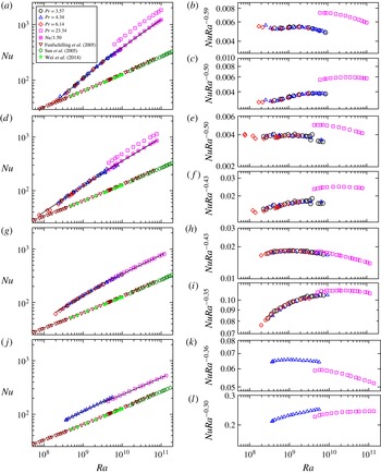
(a,d,g,j)
 $Nu$
as a function of
 $Ra$
in rough cells for (a)
 $\unicode[STIX]{x1D706}=4.0$
; (d)
 $\unicode[STIX]{x1D706}=1.9$
; (g)
 $\unicode[STIX]{x1D706}=1.0$
and (
 $j$
)
 $\unicode[STIX]{x1D706}=0.5$
. The down-pointing triangles are from Funfschilling et al. (Reference Funfschilling, Brown, Nikolaenko and Ahlers2005) (
 $\unicode[STIX]{x1D6E4}=1.0,Pr=4.38$
), the hexagons are from Sun et al. (Reference Sun, Ren, Song and Xia2005) (
 $\unicode[STIX]{x1D6E4}=2.0,Pr=4.34$
) and the stars are from Wei et al. (Reference Wei, Chan, Ni, Zhao and Xia2014) (
 $\unicode[STIX]{x1D6E4}=1.0,Pr=4.38$
). Data at
 $Pr=4.34$
in
 $(j)$
are from Wei et al. (Reference Wei, Chan, Ni, Zhao and Xia2014);
 $Nu$
at
 $Pr=23.34$
at
 $\unicode[STIX]{x1D706}=4.0$
and 1.9 are larger than those at
 $Pr=3.57$
at the same
 $Ra$
. For a better comparison, they are shifted downwards respectively by 1.5 and 1.34 and displayed using squares with a cross. The solid lines are power-law fits to the data larger and smaller than
 $Ra^{\ast }\sim 4\times 10^{9}$
. (b,c,e,f,h,i,k,l) The compensated plots of
 $Nu$
with the fitted
 $Ra$
scaling for
 $Ra$
larger and smaller than
 $Ra\sim 4\times 10^{9}$
from (a,d,g,j).

Figure 4(a,d,g,j) shows
 $Nu$
as a function of
 $Ra$
and
 $Pr$
in rough cells with
 $\unicode[STIX]{x1D706}=4.0,1.9,1.0$
and 0.5, respectively. The solid lines in the figure are power-law fit to each data set for
 $Ra$
larger and smaller than a critical Rayleigh number
 $Ra^{\ast }=4\times 10^{9}$
. The same data from smooth cells as shown in figure 3 are shown in these figures. The general conclusion that one can draw from these figures is that the heat transport is enhanced in rough cells.
We first discuss the case with
 $\unicode[STIX]{x1D706}=1.0$
(figure 4
g). Within the precision of the experiments, data at different values of
 $Pr$
but the same
 $Ra$
collapse onto each other, suggesting that the
 $Pr$
-dependence in the rough cell with
 $\unicode[STIX]{x1D706}=1.0$
is very weak in the present parameter range, which is consistent with observation in a smooth cell (Xia, Lam & Zhou Reference Xia, Lam and Zhou2002). Detailed examination of the data shows that there is a transition of the
 $Nu$
–
 $Ra$
scaling at
 $Ra^{\ast }\sim 4\times 10^{9}$
. Below and above
 $Ra^{\ast }$
, the data can be fitted by different scaling laws, i.e.
 $Nu\sim Ra^{0.43\pm 0.01}$
and
 $Nu\sim Ra^{0.35\pm 0.01}$
. The different scaling laws suggest that the heat transport enhancement regime in a rough cell can be further classified into two regimes for the
 $Pr$
range covered in the present experiments. We term the two regimes before and after
 $Ra^{\ast }$
as Regime II and Regime III. The data are compensated by the scaling exponents in Regimes II and III and shown in figure 4(h,i). A gradual transition at
 $Ra^{\ast }\sim 4\times 10^{9}$
is clearly seen.
Data at
 $\unicode[STIX]{x1D706}=4.0,1.9$
and 0.5 are plotted in figure 4(a,d,j). One interesting feature revealed in figure 4(a,d) is that the
 $Nu$
at
 $Pr=23.34$
is larger than that at
 $Pr=3.57$
when
 $Ra$
is the same. We note that this
 $Nu$
-enhancement for FC770 (
 $Pr=23.34$
), as compared to water (
 $Pr=3.57$
), only occurs for the large
 $\unicode[STIX]{x1D706}$
cases. In fact, for the smallest value of
 $\unicode[STIX]{x1D706}$
(
 $=0.5$
) there is a slight decrease in
 $Nu$
. This is quite surprising and unexpected, as in the case of a smooth cells,
 $Nu$
peaks around
 $Pr=3\sim 4$
(Xia et al.
Reference Xia, Lam and Zhou2002). It is not clear why the heat transport enhancement in rough cells has this peculiar
 $Pr$
-dependence, and furthermore this behaviour has a strong
 $\unicode[STIX]{x1D706}$
dependence, i.e. it is 150 % for
 $\unicode[STIX]{x1D706}=4.0$
, 134 % for
 $\unicode[STIX]{x1D706}=1.9$
, 4 % for
 $\unicode[STIX]{x1D706}=1.0$
and
 $-8\,\%$
for
 $\unicode[STIX]{x1D706}=0.5$
. One possible reason leading to such a
 $Pr$
-abnormality is that the lifetime of the thermal plumes at larger
 $Pr$
is larger compared to the small
 $Pr$
case. Assuming that the thermal plumes have typical length scale comparable to the thermal BL thickness, the estimated thermal diffusion time scale, i.e.
 $\unicode[STIX]{x1D6FF}_{th}^{2}/\unicode[STIX]{x1D705}$
, for FC770 is 14.5 s and that for water is 2.6 s at
 $Ra\approx 10^{10}$
. When normalised by the LSC turnover time, the dimensionless plume lifetime for FC770 is 0.25 and that for water is 0.11 for
 $\unicode[STIX]{x1D706}=4.0$
. Another likely reason is the stronger plume clustering effect in rough cells with larger
 $\unicode[STIX]{x1D706}$
as shown by the shadowgraph images in figure 16, which also has the effect of increasing plume lifetime or slowing the decay of plumes. While it is difficult to quantify the combined effect of these two factors, it appears that larger values of
 $\unicode[STIX]{x1D706}$
together with a larger
 $Pr$
result in a more efficient enhancement in the heat transport. For small
 $\unicode[STIX]{x1D706}$
and/or small
 $Pr$
, thermal plumes lose more heat to the surrounding fluid and therefore
 $Nu$
will not be enhanced as much.
To determine more accurately the scaling law of
 $Nu$
versus
 $Ra$
, the data at
 $Pr=23.34$
in figure 4(a,d) are shifted downwards by a constant, i.e. 1.50 in (a) and 1.34 in (d), to collapse data at different
 $Pr$
but the same
 $Ra$
. The transition of the heat transport scaling around
 $Ra^{\ast }$
is observed for all
 $\unicode[STIX]{x1D706}$
studied. The power-law fits of
 $Nu=ARa^{\unicode[STIX]{x1D6FC}}$
in Regimes II and III for different values of
 $\unicode[STIX]{x1D706}$
are summarised in table 1. It should be noted that the shifted high
 $Pr$
data were included in the fitting. Since
 $Ra$
obtained using water as working fluid at
 $Pr=3.57$
and that using FC770 as working fluid at
 $Pr=23.34$
had an overlapping range of less than a half-decade, i.e. from
 $6\times 10^{9}$
to
 $9\times 10^{9}$
, a determination of the
 $Pr$
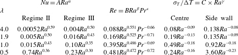
dependence in Regime III was not possible in the present experiments. It is seen that the heat transport law is distinctively different in Regime II and Regime III. This can be seem more clearly from the compensated plot in the right panel next to figure 4(a,d,j).
The experimentally determined scaling exponent
 $\unicode[STIX]{x1D6FC}$
, i.e.
 $Nu\sim Ra^{\unicode[STIX]{x1D6FC}}$
, in both Regime II and Regime III increases significantly with
 $\unicode[STIX]{x1D706}$
. In Regime II, the
 $\unicode[STIX]{x1D6FC}$
increases from 0.36 to 0.59 when
 $\unicode[STIX]{x1D706}$
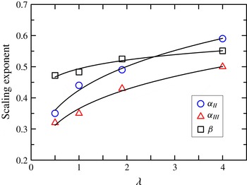
is increased from 0.5 to 4.0; and in Regime III, it increases from 0.30 to 0.50. These data are plotted in figure 5. If a power-law fit is attempted with these data within the limited range of
 $\unicode[STIX]{x1D706}$
, we obtain
 $\unicode[STIX]{x1D6FC}_{II}=0.42\unicode[STIX]{x1D706}^{0.23\pm 0.02}$
and
 $\unicode[STIX]{x1D6FC}_{III}=0.35\unicode[STIX]{x1D706}^{0.24\pm 0.02}$
which are shown as solid lines in the figure. Within the error bar, the
 $\unicode[STIX]{x1D706}$
-dependences of
 $\unicode[STIX]{x1D6FC}_{II}$
and
 $\unicode[STIX]{x1D6FC}_{III}$
are the same except that the prefactor of
 $\unicode[STIX]{x1D6FC}_{II}$
is larger than
 $\unicode[STIX]{x1D6FC}_{III}$
. The results suggest that the scaling law of the heat transport in turbulent RBC over rough plates can be manipulated using
 $\unicode[STIX]{x1D706}$
. In this sense, the present experiments demonstrate clearly the importance of roughness geometry on turbulent heat transport. Any realistic model for turbulent thermal convection in nature should take into account the effects of wall roughness.
Very recently, it has been found that there is an upper bound for the heat transport in turbulent convection over rough plates, i.e.
 $Nu$
cannot grow faster than
 $Nu\sim Ra^{1/2}$
in the limit of
 $Ra\rightarrow \infty$
(Goluskin & Doering Reference Goluskin and Doering2016). With increasing
 $Ra$
, Regime II is just a transient and Regime III is the dominant one. Our experiments showed that at
 $\unicode[STIX]{x1D706}=4.0$
the scaling exponent already reached 0.50, which was consistent with the upper bound derived (Goluskin & Doering Reference Goluskin and Doering2016). One interesting question is whether the scaling exponent will saturate to 0.50 with further increasing
 $\unicode[STIX]{x1D706}$
which is very challenging to achieve experimentally due to technical difficulties in machining the plates. DNS studies may provide helpful insights into this aspect of the problem.
Measured scaling law of the Nusselt number
 $Nu$
and normalised temperature fluctuations
 $\unicode[STIX]{x1D70E}_{T}/\unicode[STIX]{x0394}T$
in Regime III for different values of
 $\unicode[STIX]{x1D706}$
.

We next study the
 $\unicode[STIX]{x1D706}$
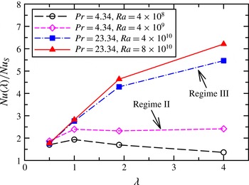
-dependence of the heat transport enhancement in Regime II and Regime III. Figure 6 shows the heat transport enhancement in rough cells compared with that in a smooth cell. It is seen that the heat transport enhancement in Regime II (open symbols in figure 6) first increases and then decreases with increasing
 $\unicode[STIX]{x1D706}$
. The situation is very different in Regime III (solid symbols in figure 6) where it is found that the heat transport enhancement increases monotonically with increasing
 $\unicode[STIX]{x1D706}$
. A maximum heat transport enhancement of 637 % is observed at
 $\unicode[STIX]{x1D706}=4.0$
.
We note that in a DNS study, Wagner & Shishkina (Reference Wagner and Shishkina2015) show that the heat transport is enhanced more for slender roughness elements, i.e. larger
 $\unicode[STIX]{x1D706}$
, using only four roughness elements with a roughness height of 0.125H (‘obstacles’ in Wagner & Shishkina Reference Wagner and Shishkina2015) in a quasi-2-D convection cell. The observation in Wagner & Shishkina (Reference Wagner and Shishkina2015) is qualitatively in agreement with what we find here, e.g. heat transport enhancement generally increases with
 $\unicode[STIX]{x1D706}$
(see e.g. figure 6).
3.2 Transition from Regime II to Regime III: the viscous boundary layer cross-over
To understand what may have happened at
 $Ra^{\ast }$
, i.e. the transition from Regime II to Regime III, we recall that there are two types of BLs in turbulent RBC, i.e. the thermal BL and the viscous BL. The viscous BL is thicker than the thermal BL for
 $Pr>1$
. According to the Grossmann–Lohse model for turbulent RBC, BLs play crucial role in determine the global heat transport (Grossmann & Lohse Reference Grossmann and Lohse2000). The transition seen in figure 4 may be understood in terms of the viscous BL cross-over, i.e. the roughness elements not only strongly perturb the thermal BL but also alter the viscous BL in Regime III. To verify this, we directly measured the viscous boundary layer in the rough cell with
 $\unicode[STIX]{x1D706}=1.0$
.
The scaling exponent
 $\unicode[STIX]{x1D6FC}$
from power-law fits to
 $Nu$
versus
 $Ra$
, i.e.
 $Nu\sim Ra^{\unicode[STIX]{x1D6FC}}$
, in Regime II (circles) and Regime III (triangles) as a function of
 $\unicode[STIX]{x1D706}$
. Also plotted in the figure is the scaling exponent
 $\unicode[STIX]{x1D6FD}$
from power-law fits to
 $Re$
versus
 $Ra$
(squares), i.e.
 $Re\sim Ra^{\unicode[STIX]{x1D6FD}}$
, as a function of
 $\unicode[STIX]{x1D706}$
. The solids lines are empirical power-law fits to the respective data sets:
 $\unicode[STIX]{x1D6FC}_{II}=0.43\unicode[STIX]{x1D706}^{0.24\pm 0.02}$
,
 $\unicode[STIX]{x1D6FC}_{III}=0.37\unicode[STIX]{x1D706}^{0.23\pm 0.02}$
and
 $\unicode[STIX]{x1D6FD}=0.49\unicode[STIX]{x1D706}^{0.08\pm 0.01}$
.

The heat transport enhancements in Regime II (open symbols) and Regime III (solid symbols) as a function of
 $\unicode[STIX]{x1D706}$
.

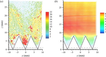
The instantaneous (a) and time-averaged (b) velocity fields measured near the bottom plate within the large-scale circulation plane (
 $Ra=4.22\times 10^{9}$
,
 $Pr=4.34$
and
 $\unicode[STIX]{x1D706}=1.0$
). The velocity magnitude (in units of
 $\text{mm}~\text{s}^{-1}$
) is colour coded with the colour bar nearby each figure and is also represented by the length of the vectors. The velocity field is not accessible experimentally below the dashed lines.

(a) Typical time-averaged horizontal velocity
 $U$
and root-mean-square horizontal velocity
 $\unicode[STIX]{x1D70E}_{u}$
profiles (
 $Ra=4.22\times 10^{9}$
,
 $\unicode[STIX]{x1D706}=1.0$
and
 $Pr=4.34$
). The vertical dashed line indicates the location of the viscous boundary layer. (b) Normalised viscous boundary layer thickness
 $\unicode[STIX]{x1D6FF}_{v}/H$
versus
 $Ra$
. The dashed line marks the height of the roughness elements. The datum at the highest
 $Ra$
(symbols with cross,
 $\unicode[STIX]{x0394}T=29.83~\text{K}$
) shows different behaviours with other data points which we believe is an artefact due to the strong optical distortion of the images used for PIV analysis.

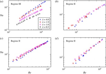
 $Nu$
as a function of
 $Re$
measured in rough cells with different values of
 $\unicode[STIX]{x1D706}$
at (a)
 $Pr=23.34$
(b)
 $Pr=6.14$
(c)
 $Pr=4.34$
and (d)
 $Pr=3.57$
.

An example of the instantaneous velocity map measured at
 $Ra=4.22\times 10^{9}$
and
 $Pr=4.34$
is shown in figure 7(a). The triangles outline the space occupied by the roughness elements schematically. The velocity magnitude is coded by both the colour and the length of the vectors. The instant velocity field shows that the mean flow is going from the right to the left and there are intermittent bursts of the flow velocity. Figure 7(b) depicts the time-averaged velocity field with the velocity magnitude coded also in both colour and the length of the vectors. One may notice that the time-averaged maximum velocity magnitude is significantly reduced when compared with the instantaneous one as revealed by the scale bars. After averaging over time one sees that the mean velocity is uniform with respect to
 $x$
except very close to the plate, e.g. in between the roughness elements. A tiny counter-rotating vortex may be identified in the region
 $-8~\text{mm}<x<-5~\text{mm}$
and
 $0~\text{mm}<z<4~\text{mm}$
. The mean velocity field varied weakly with
 $x$
(figure 7
b). We thus averaged the mean velocity field along
 $x$
-direction to obtain the mean velocity and the root-mean-square (r.m.s.) velocity profiles.
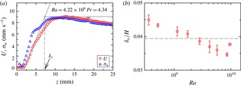
Figure 8(a) shows an example of the horizontal mean velocity profile
 $U(z)$
and the profile of the r.m.s. velocity
 $\unicode[STIX]{x1D70E}_{U}(z)$
measured at
 $Ra=4.22\times 10^{9}$
and
 $Pr=4.34$
. A remarkable feature shown in figure 8(a) is that the r.m.s. velocity is comparable to the mean velocity very close to the plate, and it is even larger than the mean velocity within the viscous BL. The origin of the enhanced velocity fluctuation is not clear but speculatively this should largely correlate with the intermittent bursts of thermal plumes. In contrast, the maximum r.m.s. velocity in a smooth cell is only approximately 30 % of the maximum mean velocity and it is always smaller than the mean velocity within the BL region (Sun, Cheung & Xia Reference Sun, Cheung and Xia2008; Wei & Xia Reference Wei and Xia2013).
The viscous BL thickness was determined using the so-called slope method: the intersection between the extrapolation of the linear part of the velocity profile very close to the plate and the maximum mean horizontal velocity was defined as the thickness of the viscous boundary layer
 $\unicode[STIX]{x1D6FF}_{v}$
(indicated by the vertical dashed line in figure 8
a) (Xin, Xia & Tong Reference Xin, Xia and Tong1996; Xin & Xia Reference Xin and Xia1997; Qiu & Xia Reference Qiu and Xia1998; Sun et al.
Reference Sun, Cheung and Xia2008; Wei & Xia Reference Wei and Xia2013). The
 $Ra$
-dependence of the viscous BL thickness normalised by the height of the convection cell is plotted in figure 8(b). With increasing
 $Ra$
,
 $\unicode[STIX]{x1D6FF}_{u}/H$
becomes thinner and thinner. At
 $Ra\sim 3\times 10^{9}$
,
 $\unicode[STIX]{x1D6FF}_{u}/H$
approximately equals to
 $h/H$
. This roughly corresponds to
 $Ra^{\ast }$
seen in the measured
 $Nu$
(
 $Ra^{\ast }\sim 4\times 10^{9}$
). This observation indicates that the transition of the heat transport law between Regimes II and III may be caused by the viscous BL becoming smaller than the height of the roughness elements. After this viscous BL cross-over, the roughness elements strongly perturb both the thermal and the viscous BLs. The thermal plumes emitted from the tip of pyramids can then be directly ejected into the bulk. For
 $Pr=23.34$
, the estimated viscous BL thickness at the smallest
 $Ra$
explored in the experiments (
 $Ra=4.39\times 10^{9}$
) was 0.04H (Lam et al.
Reference Lam, Shang, Zhou and Xia2002), which was very close to the height of the roughness element, implying that the measurements with
 $Pr=23.34$
were all in Regime III.
In the asymptotically large
 $Ra$
limit, the thickness of the BLs is so small such that the roughness elements perturb both the thermal and the viscous BLs. The system is in Regime III in this case wherein
 $Nu$
is very sensitive to the LSC, or equivalently to the Reynolds number
 $Re$
associated with the LSC (to be defined in § 3.3). We plot in figure 9
 $Nu$
as a function of
 $Re$
for (a)
 $Pr=23.34$
, (b)
 $Pr=6.14$
, (c)
 $Pr=4.34$
and (d)
 $Pr=3.57$
. On one hand, figure 9(a) shows that
 $Nu$
increases with
 $\unicode[STIX]{x1D706}$
for all
 $Re$
measured at
 $Pr=23.34$
, which are in the Regime III. On the other hand,
 $Nu$
at other
 $Pr$
where mostly within the Regime II shows weak dependence on
 $Re$
. This is another evidence supporting that the viscous BL cross-over may also play important role in turbulent thermal convection with roughness elements.
3.3 Reynolds number measurements
The self-organised large-scale circulation (or ‘wind of turbulence’) is one of the fascinating features of turbulent RBC. The flow dynamics of the LSC is characterised by the associated Reynolds number
 $Re$
. We study in this section how the roughness geometry alters the dynamics of the LSC by examining the
 $Re$
dependence on both
 $Ra$
and
 $Pr$
. It has been well known that there exists a well-defined low-frequency oscillation in turbulent RBC. The time scale of this oscillation is interpreted as the turnover time
 $T_{f}$
of the LSC (see, e.g. Xie, Wei & Xia (Reference Xie, Wei and Xia2013) and references therein). By choosing a typical length scale of the LSC, e.g.
 $4H$
, the Reynolds number is calculated as:
 $$\begin{eqnarray}Re=UH/\unicode[STIX]{x1D708}=4H^{2}/(T_{f}\unicode[STIX]{x1D708}).\end{eqnarray}$$
Time-resolved temperature signals measured
 ${\sim}1~\text{cm}$
away from the side wall were used to determine
 $T_{f}$
and thus the
 $Re$
as a function of
 $Ra$
and
 $Pr$
when changing the roughness geometry, i.e. at different values of
 $\unicode[STIX]{x1D706}$
. The turnover time of the LSC was determined by locating the time position of the first peak of the temperature autocorrelation function
 $C(\unicode[STIX]{x1D70F})$
, which is defined as:
 $$\begin{eqnarray}C(\unicode[STIX]{x1D70F})=\frac{\langle [T(t+\unicode[STIX]{x1D70F})-\langle T(t)\rangle _{t}][T(t)-\langle T(t)\rangle _{t}]\rangle _{t}}{\unicode[STIX]{x1D70E}_{T}^{2}},\end{eqnarray}$$
where
 $\langle \cdots \rangle _{t}$
denotes time averaging and
 $\unicode[STIX]{x1D70E}_{T}$
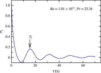
is the r.m.s. temperature. An example of the autocorrelation function measured in a convection cell with
 $\unicode[STIX]{x1D706}=4.0$
at
 $Ra=1.01\times 10^{11}$
and
 $Pr=23.34$
is depicted in figure 10. Clear oscillations can be seen from
 $C(\unicode[STIX]{x1D70F})$
. Fitting the data points nearby the first peak of
 $C(\unicode[STIX]{x1D70F})$
with a sixth-order polynomial, the time location of the first peak was determined and denoted as
 $T_{f}$
. The uncertainty of
 $T_{f}$
was from
 $0.06$
s to
 $0.008$
s with increasing
 $Ra$
.
Autocorrelation function of the temperature measured
 ${\sim}1$
cm away from side wall in a rough cell with
 $\unicode[STIX]{x1D706}=4.0$
at
 $Ra=1.01\times 10^{11}$
and
 $Pr=23.34$
. Here
 $T_{f}$
is the turnover time of the LSC.

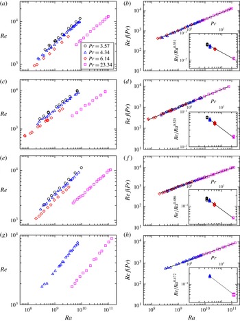
Reynolds number
 $Re$
as a function of
 $Ra$
and
 $Pr$
in rough cells for (a)
 $\unicode[STIX]{x1D706}=4.0$
, (c)
 $\unicode[STIX]{x1D706}=1.9$
, (e)
 $\unicode[STIX]{x1D706}=1.0$
and (g)
 $\unicode[STIX]{x1D706}=0.5$
. To determine more precisely the scaling exponent of
 $Re$
with respect to
 $Ra$
, data measured at
 $Pr=3.53,4.34$
and
 $6.14$
in (a,c,e,g) are multiplied by a
 $Pr$
-dependent constant
 $f(Pr)$
to collapse with data at
 $Pr=23.34$
. The shifted data are shown in the main plot in the right panels (b,d,f,g) with power-law fit
 $Re\,f(Pr)\sim Ra^{\unicode[STIX]{x1D6FD}}$
shown as solid lines. The insets in (b,d,f,g) show the compensated plot
 $ReRa^{-\unicode[STIX]{x1D6FD}}$
with respect to
 $Pr$
with the solid lines representing power-law fits to the data. See table 1 for the fitted power laws.

Figure 11 displays
 $Re$
as a function of
 $Ra$
and
 $Pr$
in rough cells with
 $\unicode[STIX]{x1D706}=4.0$
(a,b),
 $\unicode[STIX]{x1D706}=1.9$
(c,d),
 $\unicode[STIX]{x1D706}=1.0$
(e,f) and
 $\unicode[STIX]{x1D706}=0.5$
(g,h). Let us first discuss the case for
 $\unicode[STIX]{x1D706}=4.0$
. The
 $Re$
as a function of
 $Ra$
for
 $Pr=3.57,4.34,6.14$
and
 $23.34$
are plotted in figure 11(a) on a log–log scale. The
 $Re$
exhibits power-law dependence on
 $Ra$
at different
 $Pr$
, i.e.
 $Re\sim Ra^{\unicode[STIX]{x1D6FD}}$
. To determine more precisely
 $\unicode[STIX]{x1D6FD}$
, data at
 $Pr=3.57$
, 4.34 and 6.14 were multiplied by a
 $Pr$
-dependent constant to collapse them with data at
 $Pr=23.34$
onto a single line. The shifted data are shown in the main plot of figure 11(b). A power-law fit to the data over almost three decades of
 $Ra$
yielded:
 $Re\sim Ra^{0.551\pm 0.001}$
. The
 $Ra$
-dependence of
 $Re$
was then divided out by compensating the data in figure 11(a) with the so-determined power law, e.g. the inset of figure 11(b). Within a relatively limited range of
 $Pr$
, the data can also be described by a power law, i.e.
 $Re/Ra^{0.551}\sim Pr^{-0.66\pm 0.02}$
. The so-determined
 $Re(Ra,Pr)$
is:
 $$\begin{eqnarray}Re=0.088Ra^{0.551}Pr^{-0.66}\quad (\unicode[STIX]{x1D706}=4.0).\end{eqnarray}$$
Applying the same procedure to data obtained in rough cells with
 $\unicode[STIX]{x1D706}=1.9$
(figure 11
c),
 $\unicode[STIX]{x1D706}=1.0$
(figure 11
e) and
 $\unicode[STIX]{x1D706}=0.5$
(figure 11
g), we determined the
 $Ra$
and
 $Pr$
dependence of
 $Re$
for each values of
 $\unicode[STIX]{x1D706}$
, respectively. The scaling laws of
 $Re=BRe^{\unicode[STIX]{x1D6FD}}Pr^{\unicode[STIX]{x1D716}}$
for different values of
 $\unicode[STIX]{x1D706}$
are summarised in table 1.
On one hand, with
 $\unicode[STIX]{x1D706}$
increasing from 0.5 to 4.0 the scaling exponent
 $\unicode[STIX]{x1D6FD}$
, i.e.
 $Re\sim Ra^{\unicode[STIX]{x1D6FD}}$
, increases from 0.472 to 0.551, which is plotted as a function of
 $\unicode[STIX]{x1D706}$
in figure 5. The data may be described by an empirical power law within a very limited range of
 $\unicode[STIX]{x1D706}$
, i.e.
 $\unicode[STIX]{x1D6FD}=0.49\unicode[STIX]{x1D706}^{0.08\pm 0.01}$
. On the other hand, the scaling exponent
 $\unicode[STIX]{x1D716}$
, i.e.
 $Re\sim Pr^{\unicode[STIX]{x1D716}}$
, remains at the same value around
 $-0.70$
within experimental uncertainty except for
 $\unicode[STIX]{x1D706}=4.0$
. Whether there is a change of the
 $Pr$
-dependence of
 $Re$
in the rough cell with
 $\unicode[STIX]{x1D706}=4.0$
requires future investigation with a wider range of
 $Pr$
. The change of
 $\unicode[STIX]{x1D6FD}$
with
 $\unicode[STIX]{x1D706}$
suggests a change of the LSC dynamics when the geometry of the roughness elements is changed. It is thus interesting to study torsional and sloshing oscillations of the LSC dynamics in rough cells with different values of
 $\unicode[STIX]{x1D706}$
as compared to those oscillations in a smooth cell (Funfschilling & Ahlers Reference Funfschilling and Ahlers2004; Xi et al.
Reference Xi, Zhou, Zhou, Chan and Xia2009; Xie et al.
Reference Xie, Wei and Xia2013). This is beyond the scope of the present studies and will be investigated in the future. Interestingly, the transition of the heat transport scaling law from Regime II to Regime III does not present in the Reynolds number measurement.
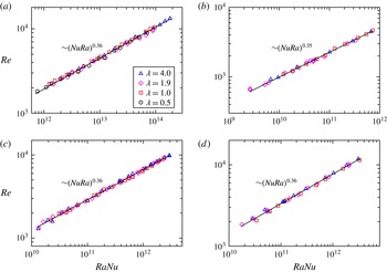
Reynolds number
 $Re$
as a function of
 $RaNu$
for different values of
 $\unicode[STIX]{x1D706}$
with the solid line representing a power-law fit to the data irrespective of
 $\unicode[STIX]{x1D706}$
. (a)
 $Pr=23.34$
and
 $Re=0.076\times (RaNu)^{0.36\pm 0.01}$
; (b)
 $Pr=6.14$
and
 $0.266\times (RaNu)^{0.35\pm 0.01}$
; (c)
 $Pr=4.34$
and
 $0.281\times (RaNu)^{0.36\pm 0.01}$
; (d)
 $Pr=3.57$
and
 $Re=0.340\times (RaNu)^{0.36\pm 0.01}$
.

It is found very recently that
 $Re$
is insensitive to the plate morphology for a given input heat flux for
 $\unicode[STIX]{x1D706}=0$
and 0.5 (Wei et al.
Reference Wei, Chan, Ni, Zhao and Xia2014), i.e. when
 $Re$
is plotted against the flux Rayleigh number
 $RaNu$
, data at different values of
 $\unicode[STIX]{x1D706}$
collapse. We plot
 $Re$
as a function of
 $RaNu$
for different values of
 $\unicode[STIX]{x1D706}$
and
 $Pr$
in figure 12. The data at the same
 $Pr$
but different
 $\unicode[STIX]{x1D706}$
indeed overlap which is in agreement with the observation in Wei et al. (Reference Wei, Chan, Ni, Zhao and Xia2014), but now for a wider range of
 $\unicode[STIX]{x1D706}$
and
 $Pr$
. In addition, data at the same
 $Pr$
can be fitted by a power law, i.e.
 $Re=0.076\times (RaNu)^{0.36\pm 0.01}$
 $(Pr=23.34)$
,
 $Re=0.266\times (RaNu)^{0.35\pm 0.01}$
 $(Pr=6.14)$
,
 $Re=0.281\times (RaNu)^{0.36\pm 0.01}(Pr=4.34)~$
and
 $Re=0.340\times (RaNu)^{0.36\pm 0.01}$
 $(Pr=3.57)$
. The scaling exponents of these power-law fits are the same within experimental uncertainty but the magnitudes decrease with
 $Pr$
.
3.4 Local temperature fluctuations
Since Regime II is a transitional state, we focus on temperature fluctuations measured in Regime III only. To simplify the analysis, we do not take into account the effects of
 $Pr$
and limit the analysis to measurements done in FC770 only (
 $Pr=23.34$
). The results may shed light upon the mechanism leading to the change of the heat transport scaling in rough cells with different roughness geometries in Regime III.
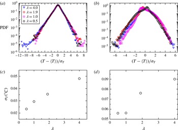
Probability density functions (PDFs) of the standardised temperature measured (a) at the cell centre and (b) near the side wall for different values of
 $\unicode[STIX]{x1D706}$
(
 $Ra=2.1\times 10^{10}$
and
 $Pr=23.34$
). The r.m.s. temperatures as a function of
 $\unicode[STIX]{x1D706}$
at the cell centre and side wall are plotted in (c) and (d), respectively.

The probability density functions (PDFs) of the standardised temperature
 $(T-\langle T\rangle )/\unicode[STIX]{x1D70E}_{T}$
measured at
 $Ra=2.1\times 10^{11}$
at four different values of
 $\unicode[STIX]{x1D706}$
at the cell centre and side wall are displayed in figures 13(a) and 13(b) respectively, where
 $\unicode[STIX]{x1D70E}_{T}$
is the r.m.s. temperature that is shown as a function of
 $\unicode[STIX]{x1D706}$
in figure 13(c,d) at the cell centre and side wall. It is seen that the PDFs at different
 $\unicode[STIX]{x1D706}$
overlap very nicely at the cell centre, suggesting that the bulk turbulence shares similar dynamics at different values of
 $\unicode[STIX]{x1D706}$
. A notable feature seen in figure 13(a) is that the PDFs are significantly skewed toward the negative side, i.e. more cold plumes are detected in the cell centre than hot ones. This feature has not been observed either by us or reported by others in smooth cells with the same boundary conditions, i.e. constant temperature at the top boundary and constant heat flux at the bottom boundary. Thus, the reason for this phenomenon remains unknown to us at present. At the side wall, the shapes of the PDFs remain approximately invariant with
 $\unicode[STIX]{x1D706}$
except the case with
 $\unicode[STIX]{x1D706}=0.5$
. For measurements with
 $\unicode[STIX]{x1D706}=0.5$
the thermistor was positioned such that the upwelling hot plumes of the LSC were detected, while for the other cases the downwelling cold plumes of the LSC were detected. The positive tails of the PDFs overlap well onto each other while the negative tails, especially those larger than
 $3\unicode[STIX]{x1D70E}_{T}$
, change with
 $\unicode[STIX]{x1D706}$
. As the large temperature fluctuations are caused by thermal plumes, this observation suggests a change of the plume dynamics with increasing
 $\unicode[STIX]{x1D706}$
. The r.m.s. temperature at the cell centre increases considerably with
 $\unicode[STIX]{x1D706}$
as can be seen from figure 13(c), and that at the side wall first remains almost the same for
 $\unicode[STIX]{x1D706}=0.5$
and 1.0 and then increases with
 $\unicode[STIX]{x1D706}$
as well.
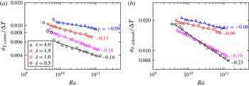
 $\unicode[STIX]{x1D706}$
-dependence of the normalised r.m.s. temperature as a function of
 $Ra$
at (a) the cell centre and (b) the side wall. The solid lines are power-law fits to the individual data set with the scaling exponents displayed nearby each data set. The data are measured at
 $Pr=23.34$
.

The Rayleigh number dependence of normalised r.m.s. temperatures
 $\unicode[STIX]{x1D70E}_{T}/\unicode[STIX]{x0394}T$
for different values of
 $\unicode[STIX]{x1D706}$
measured at the cell centre and near the side wall are shown in figures 14(a) and 14(b), respectively. With increasing
 $\unicode[STIX]{x1D706}$
,
 $\unicode[STIX]{x1D70E}_{T}/\unicode[STIX]{x0394}T$
enhances considerably. The changes lie not only in the magnitudes but also the scaling exponents with
 $Ra$
. The scaling exponents of the power-law fits, e.g.
 $\unicode[STIX]{x1D70E}_{T}/\unicode[STIX]{x0394}T=C\times Ra^{\unicode[STIX]{x1D6FE}}$
, are displayed nearby each data set in figure 14(a,b) and the scaling laws of each data set are summarised in table 1. The scaling exponent increases from
 $-0.16$
to
 $-0.09$
with
 $\unicode[STIX]{x1D706}$
increased from 0.5 to 4.0 in the cell centre. For comparison, Wei & Ahlers (Reference Wei and Ahlers2016) obtained an exponent of
 $-0.17$
in the centre of a smooth cell for a comparable
 $Pr$
(
 $Pr=12.3$
). With a possible
 $Pr$
-dependence of the temperature fluctuation unknown at the present, the experimental results suggest that the
 $Ra$
-dependence of the temperature fluctuation at the cell centre becomes stronger with increasing
 $\unicode[STIX]{x1D706}$
. Near the side wall, the scaling exponent increases from
 $-0.23$
to
 $-0.08$
in the
 $\unicode[STIX]{x1D706}$
range covered in the experiments, suggesting a weakened dependence of temperature fluctuation on
 $\unicode[STIX]{x1D706}$
at the side wall. To the best of our knowledge, there has been no report on the smooth cell value for this exponent in the similar
 $Pr$
range near the side wall.
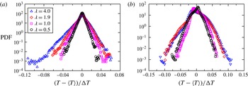
Probability density function of the temperature deviation from the mean
 $T-\langle T\rangle$
normalised by the applied temperature between the top and bottom plate
 $\unicode[STIX]{x0394}T$
at (a) the cell centre and (b) the side wall (
 $Ra=2.1\times 10^{10}$
,
 $Pr=23.34$
).

To gain further insight into the dynamics of temperature fluctuations with increasing
 $\unicode[STIX]{x1D706}$
, we examine the PDFs of the normalised temperature deviation from the mean
 $(T-\langle T\rangle )/\unicode[STIX]{x0394}T$
for different values of
 $\unicode[STIX]{x1D706}$
at
 $Ra=2.1\times 10^{10}$
at the cell centre and the side wall respectively, as displayed in figure 15(a,b). The figure reveals that large events are becoming more probable with increasing
 $\unicode[STIX]{x1D706}$
at the same
 $Ra$
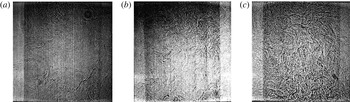
, i.e. hotter and colder plumes, suggesting that the effects of changing roughness geometry are to modify the dynamics of thermal plumes and make them more coherent and energetic (therefore decay slower). This is also supported by the shadowgraph visualisation of the flow field, such as those presented in figure 16. These images are taken at
 $Ra=1.22\times 10^{11}$
and
 $Pr=23.34$
. It is seen that, with increasing
 $\unicode[STIX]{x1D706}$
, both the density and the morphology of the thermal plumes change drastically. In the smooth cell there is a well-defined LSC with few thermal plumes passing through the cell centre (figure 16
a). In the rough cell with
 $\unicode[STIX]{x1D706}=1.0$
, more thermal plumes are passing through the cell centre (figure 16
b). In the rough cell with
 $\unicode[STIX]{x1D706}=4.0$
, thermal plumes occupy almost all the space in the convection cell (figure 16
c). Furthermore, the plumes are now packed (or clustered) much more densely. This will result in their slower decay through thermal diffusion, which explains why it is now much more probable to find large temperature excursions in the cell centre (figure 15
a).
Shadowgraph images of the instantaneous flow fields in a rough cell with (a)
 $\unicode[STIX]{x1D706}=0.0$
, (b)
 $\unicode[STIX]{x1D706}=1.0$
and (c)
 $\unicode[STIX]{x1D706}=4.0$
. The images were taken at
 $Ra=1.22\times 10^{11}$
and
 $Pr=23.34$
.

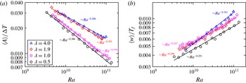
(a) The time-averaged plume amplitude
 $\langle A\rangle$
normalised by
 $\unicode[STIX]{x0394}T$
and (b) the time-averaged plume width
 $\langle w\rangle$
normalised by the large-scale circulation turnover time
 $T_{f}$
as a function of
 $Ra$
extracted from the temperature time series measured at the side wall at
 $Pr=23.34$
. The solid lines are power-law fits to individual data sets with the scaling exponents displayed nearby each data set.

To quantitatively understand the change of the dynamics of thermal plume, we extract time series of thermal plume amplitude
 $A$
and width
 $w$
using the time-resolved temperature data measured near the side wall. The detailed plume extraction method can be found in Zhou et al. (Reference Zhou, Xie, Sun and Xia2016). The normalised time-averaged plume amplitude
 $\langle A\rangle /\unicode[STIX]{x0394}T$
and normalised time-averaged plume width
 $\langle w\rangle /\unicode[STIX]{x1D70F}_{0}$
are shown in figures 17(a) and 17(b) respectively. Figure 17(a) reveals that with the increase of
 $\unicode[STIX]{x1D706}$
, the time-averaged plume amplitude
 $\langle A\rangle /\unicode[STIX]{x0394}T$
increases. The solid lines are power-law fits to the data at different values of
 $\unicode[STIX]{x1D706}$
with the scaling exponents listed nearby each data set. The scaling exponent of time-averaged plume amplitude increases from
 $-0.386$
to
 $-0.266$
with
 $\unicode[STIX]{x1D706}$
increasing from 0.5 to 4.0. In contrast, the
 $Ra$
-dependence of the time-averaged plume width remains almost the same with a scaling exponent around 0.25 for
 $\unicode[STIX]{x1D706}$
smaller than 4.0. It should be noted that the scaling exponent of plume width for
 $\unicode[STIX]{x1D706}=4.0$
increases considerably (0.341) when compared with other values of
 $\unicode[STIX]{x1D706}$
, which may be correlated with the drastically changed plume dynamics and morphology in the rough cell with
 $\unicode[STIX]{x1D706}=4.0$
. As the thermal plumes are main heat carriers in turbulent RBC, the experiments suggest that the change of plume dynamics may lead to the change of the scaling law of heat transport for different values of
 $\unicode[STIX]{x1D706}$
.
3.5 A proper parameter characterising the system:
 $\unicode[STIX]{x1D706}$
versus number density of roughness elements

When varying
 $\unicode[STIX]{x1D706}$
the number density
 $n$
of roughness elements also varies, i.e.
 $n\simeq \unicode[STIX]{x03C0}/4\unicode[STIX]{x1D6E4}^{2}\unicode[STIX]{x1D706}^{2}(H/h)^{2}$
. In fact, the two parameters have one-to-one correspondence provided that the ratio of the roughness element height
 $h$
to the cell height
 $H$
and
 $\unicode[STIX]{x1D6E4}$
are fixed, which is the case for the present study. To figure out whether
 $\unicode[STIX]{x1D706}$
is the most relevant parameter that characterises the system, we carried out another experiment, in which
 $\unicode[STIX]{x1D706}$
was kept constant at 4.0 and the height of the roughness elements was halved. Thus the number density of the roughness elements was increased by a factor of 4.
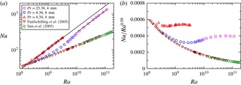
We show in figure 18(a)
 $Nu$
as a function of
 $Ra$
for measurements for
 $\unicode[STIX]{x1D706}=4.0$
rough cells with
 $h=8~\text{mm}$
and
 $h=4~\text{mm}$
together with the same smooth cell data which have be shown in figures 3 and 4. The estimated viscous boundary layer thickness at the highest
 $Ra$
reached in the experiment is 4.8 mm. Thus, the measurements at
 $Pr=23.34$
and
 $h=4~\text{mm}$
are in Regime II. A scaling exponent
 $\unicode[STIX]{x1D6FC}=0.60$
is observed in rough cell with
 $h=4~\text{mm}$
in Regime II, which is consistent with 0.59 observed in Regime II of rough cell with
 $h=8$
mm. This can be seen from the two parallel lines in figure 18(a). The similar
 $Ra$
-dependence of
 $Nu$
in Regime II in rough cells with
 $h=4$
mm and 8 mm can be seen more clearly from the compensated plot in figure 18(b). These observations suggest that
 $\unicode[STIX]{x1D706}$
is not only a suitable parameter describing the geometry of the pyramid-shaped roughness elements, but also a suitable parameter to characterise the response of turbulent RBC over rough plates with different roughness geometries.
A noticeable feature from figure 18(a) is that the measured
 $Nu$
in the rough cell with
 $h=8~\text{mm}$
is larger than that in the rough cell with
 $h=4~\text{mm}$
in Regime II despite the fact that they have similar
 $Ra$
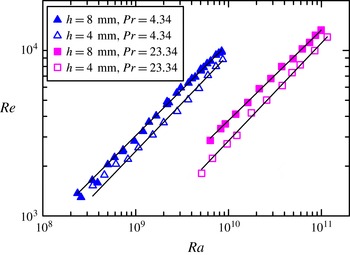
-dependence. This may be explained by the measured Reynolds number based on the circulation time of the LSC as plotted in figure 19. It is seen that
 $Re$
in the rough cell with
 $h=8~\text{mm}$
is larger than that in the rough cell with
 $h=4~\text{mm}$
, which is true for both
 $Pr=4.34$
and
 $Pr=23.34$
. The result suggests that a faster LSC can transport heat more efficiently across the convection cell.
4 Conclusion and outlook
We studied systematically in this paper the effects of roughness geometry on the global heat transport, the flow dynamics and the local temperature fluctuations in turbulent Rayleigh–Bénard convection over rough plates. The experiments were carried out in rough cells with pyramid-shaped roughness elements directly machined on the top and bottom plates. We introduced a parameter
 $\unicode[STIX]{x1D706}$
(the height of the roughness element over its base width) to characterise the geometry of the roughness element and to analyse the observed scaling behaviour of
 $Nu(Ra)$
and
 $Re(Ra,Pr)$
, where
 $Ra$
and
 $Pr$
are respectively the Rayleigh number and Prandtl number.
 $Nu$
and
 $Re$
are respectively the Nusselt number and Reynolds number. We varied
 $\unicode[STIX]{x1D706}$
from 0.5 to 4.0 by keeping the roughness height at a constant of 8 mm and changing the base width from 16 mm to 2 mm. In addition, a rough cell with
 $h=4~\text{mm}$
and
 $\unicode[STIX]{x1D706}=4.0$
was used. The experiments covered Rayleigh number
 $7.5\times 10^{5}\leqslant Ra\leqslant 1.31\times 10^{11}$
and
 $Pr$
from 3.57 to 23.34.
(a)
 $Nu$
as a function of
 $Ra$
and
 $Pr$
at fixed
 $\unicode[STIX]{x1D706}=4.0$
measured in rough cells with roughness height
 $h$
of 4 mm and 8 mm. The down-pointing triangles are from Funfschilling et al. (Reference Funfschilling, Brown, Nikolaenko and Ahlers2005) and the hexagons are from Sun et al. (Reference Sun, Ren, Song and Xia2005) for smooth cells. The solid lines are power-law fits to the respective data set. The power-law fitting in cell with
 $h=8$
mm is extrapolated to
 $Ra=2\times 10^{11}$
. (b) Compensated plot of the same data as in (a).

 $Re$
as a function of
 $Ra$
in rough cells with
 $h=8~\text{mm}$
(solid symbols) and 4 mm (open symbols) at
 $Pr=4.34$
(triangles) and 23.34 (squares), respectively. In both cells
 $\unicode[STIX]{x1D706}=4.0$
. The solid lines are power-law fits to each data set. For
 $Pr=4.34$
,
 $Re=0.028R^{0.56}$
(
 $h=8~\text{mm}$
)
 $Re=0.014R^{0.58}$
(
 $h=4~\text{mm}$
); and for
 $Pr=23.34$
 $Re=0.013R^{0.55}$
(
 $h=8~\text{mm}$
)
 $Re=0.0035R^{0.59}$
(
 $h=4~\text{mm}$
).

It is found that the heat transport is enhanced significantly by roughness elements, and the enhancement depends strongly on the roughness geometry. The heat transport scaling, i.e.
 $Nu\sim Ra^{\unicode[STIX]{x1D6FC}}$
, may be classified in to three regimes in turbulent RBC over rough plates. In Regime I, the system is in a dynamically smooth state. The heat transport scaling in a rough cell is the same as that in a smooth cell. In Regimes II and III, heat transport enhances. The scaling exponents
 $\unicode[STIX]{x1D6FC}$
of
 $Nu$
versus
 $Ra$
increase from 0.36 to 0.59 with
 $\unicode[STIX]{x1D706}$
increased from 0.5 to 4.0 in regime II, whereas it increases from 0.30 to 0.50 in Regime III. The experiment thus clearly demonstrated that the heat transport scaling in turbulent RBC could be manipulated using
 $\unicode[STIX]{x1D706}$
in Regimes II and III. The transition from Regime I to Regime II may be understood in terms of the thermal boundary layer thickness becoming smaller than the roughness height with increasing
 $Ra$
as suggested by a number of previous studies (Shen et al.
Reference Shen, Tong and Xia1996; Du et al.
Reference Du, Tong and Xia1998; Ciliberto & Laroche Reference Ciliberto and Laroche1999; Roche et al.
Reference Roche, Castaing, Chabaud and Hébral2001; Tisserand et al.
Reference Tisserand, Creyssels, Gasteuil, Pabiou, Gibert, Castaing and Chillá2011). The transition from Regime II to Regime III may be understood in terms of viscous boundary layer crossing, i.e. the viscous BL thickness becomes thinner than the height of the roughness elements, as shown by direct measurement of the viscous boundary layer profiles in the present study. When this happens, the thermal plumes emitted from the tip of the roughness can be directly ejected into the bulk flow. An unexpected
 $Pr$
effect in turbulent RBC over rough plates was also observed: larger heat transport enhancement was observed for larger values of
 $\unicode[STIX]{x1D706}$
and larger
 $Pr$
. This may be correlated with the strong clustering of thermal plumes as clearly seen from the shadowgraph visualisation of the flow field (figure 16).
The Reynolds number
 $Re$
is measured based on the turnover time of the large-scale circulation evaluated near the side wall of the cells. Both the
 $Ra$
and
 $Pr$
dependences of
 $Re$
were studied for different roughness geometries, i.e.
 $Re=B\times Ra^{\unicode[STIX]{x1D6FD}}Pr^{\unicode[STIX]{x1D716}}$
. The scaling exponent
 $\unicode[STIX]{x1D6FD}$
increased from 0.472 to 0.551 with
 $\unicode[STIX]{x1D706}$
increasing from 0.5 to 4.0, and
 $\unicode[STIX]{x1D716}$
remained at the same value around
 $-0.7$
except for the case of
 $\unicode[STIX]{x1D706}=4.0$
(
 $\unicode[STIX]{x1D716}=-0.66$
). With a limited range of
 $Pr$
, a truly increased
 $\unicode[STIX]{x1D716}$
for
 $\unicode[STIX]{x1D706}=4.0$
could not be asserted. Consistent with the observation in Wei et al. (Reference Wei, Chan, Ni, Zhao and Xia2014), it is found that
 $Re$
is insensitive to the plate morphology for a fixed flux Rayleigh number, i.e.
 $RaNu$
, but now with a wider range of
 $Pr$
and
 $\unicode[STIX]{x1D706}$
as compared with the experiment reported by Wei et al. (Reference Wei, Chan, Ni, Zhao and Xia2014).
Time-resolved local temperatures at the cell centre and side wall were measured using two small thermistors. The probability density functions of the standardised temperature
 $(T-\langle T\rangle )/\unicode[STIX]{x1D70E}_{T}$
in the cell centre remain almost invariant with respect to
 $\unicode[STIX]{x1D706}$
. The measured local temperature fluctuations at both the cell centre and side wall increase considerably with
 $\unicode[STIX]{x1D706}$
. The scaling exponent of the normalised r.m.s. temperature (
 $\unicode[STIX]{x1D70E}_{T}/\unicode[STIX]{x0394}T$
) with
 $Ra$
increases from
 $-0.16$
to
 $-0.09$
at the cell centre and from
 $-0.23$
to
 $-0.08$
at the side wall with
 $\unicode[STIX]{x1D706}$
increased from 0.5 to 4.0. By extracting thermal plume amplitude and width using a method described in Zhou et al. (Reference Zhou, Xie, Sun and Xia2016), it is found that both the plume amplitude and width increase with
 $\unicode[STIX]{x1D706}$
. The scaling exponent of time-averaged plume amplitude increases from
 $-0.386$
to
 $-0.266$
with
 $\unicode[STIX]{x1D706}$
increasing from 0.5 to 4.0. The scaling exponent for the time-averaged plume width remains at the same value around 0.25 except for the case of
 $\unicode[STIX]{x1D706}=4.0$
which is
 $-0.34$
. As thermal plumes are the main heat carriers in turbulent RBC, the experiments suggested that the change of thermal plume dynamics might be a possible reason leading to the change of the heat transport scalings in Regime III.
The experiments demonstrated clearly that the heat transport behaviour in turbulent thermal convection can be manipulated by changing the roughness geometry. It further showed that the flow dynamics and local temperature fluctuations are also altered by changing the roughness geometry. There are several open questions: What is the effect of
 $\unicode[STIX]{x1D706}$
on the dynamics of the large-scale circulation, e.g. twisting/sloshing oscillation, flow cessation/reversal? How will the vertical mean and variance temperature profiles change with
 $\unicode[STIX]{x1D706}$
?
Finally, we remark that the 0.5 scaling exponent observed for
 $\unicode[STIX]{x1D706}=4.0$
in Regime III reminds one of the Kraichnan ultimate regime of turbulent convection (Kraichnan Reference Kraichnan1962). Whether Regime III for
 $\unicode[STIX]{x1D706}=$
4.0 really corresponds to the Kraichnan regime needs further investigation. The place to look would be the boundary layer, i.e. a truly turbulent boundary layer should be the ultimate test for the Kraichnan regime. A very recent DNS study suggests roughness may be used as a route to trigger the transition to the ultimate state of turbulent convection (Toppaladoddi et al.
Reference Toppaladoddi, Succi and Wettlaufer2017). If this is indeed the case, then the dynamics of turbulent convection in the Kraichnan regime may be studied in a Rayleigh number range that is accessible using classical fluids like water in a table top experiment.
Acknowledgements
We thank Y.-H. He for help with the experiment. This work is supported by the Hong Kong Research Grants Council under grant nos. CUHK1430115 and CUHK404513.