




1 Introduction
1.1 Extreme nonlinear pulse compression concept
Since the invention of chirped pulse amplification (CPA), the peak powers and intensities of ultrashort laser pulses have continuously been increased, reaching today at large-scale facilities up to petawatts and more than
${10}^{22}$
 W/cm2, respectively[
Reference Mourou1]. The most intense lasers run, however, only at very low shot rates, which restricts their applicability. Therefore, the concurrent scaling of both peak and average power has been proclaimed as the main objective of the so-called ‘third generation femtosecond technology’[
Reference Fattahi, Barros, Gorjan, Nubbemeyer, Alsaif, Teisset, Schultze, Prinz, Haefner, Ueffing, Alismail, Vámos, Schwarz, Pronin, Brons, Geng, Arisholm, Ciappina, Yakovlev, Kim, Azzeer, Karpowicz, Sutter, Major, Metzger and Krausz2]. For this purpose, the conventional laser materials for ultra-intense light sources, namely Ti:sapphire and large aperture Nd:doped glasses, are very difficult to use because of their unfavorable thermal properties. Alternatively, optical parametric chirped pulse amplifiers (OPCPAs) are used to minimize heat generation in the amplifier crystals at the expense of zero storage time and moderate quantum efficiencies[
Reference Fattahi, Barros, Gorjan, Nubbemeyer, Alsaif, Teisset, Schultze, Prinz, Haefner, Ueffing, Alismail, Vámos, Schwarz, Pronin, Brons, Geng, Arisholm, Ciappina, Yakovlev, Kim, Azzeer, Karpowicz, Sutter, Major, Metzger and Krausz2]. Intense multi-kHz repetition rate sources are most often based on Yb-based amplifiers. Yb-lasers offer excellent average power scalability through fiber, innoslab or thin-disk geometries[
Reference Zuo and Lin3]. Furthermore, up to 720 mJ pulse energy at sub-ps pulse durations was achieved with thin-disk amplifiers[
Reference Herkommer, Krötz, Jung, Klingebiel, Wandt, Bessing, Walch, Produit, Michel, Bauer, Kienberger and Metzger4], but pulse energies exceeding 1 J have not been demonstrated with ultrafast room-temperature ytterbium-doped yttrium aluminum garnet (Yb:YAG) lasers so far.
Here, we propose a CPA-free ultrashort pulse generation scheme that relies on gain media that provide both the capability to generate joule-level pulse energies and to handle kilowatts of average powers, for example, neodymium-doped yttrium aluminum garnet (Nd:YAG)[ Reference Fan, Qiu, Kang, Chen, Ge and Tang5], cryogenically cooled Yb:YAG[ Reference Wang, Chi, Baumgarten, Dehne, Meadows, Davenport, Murray, Reagan, Menoni and Rocca6, Reference De Vido, Quinn, Clarke, McHugh, Mason, Spear, Smith, Divoky, Pilar, Denk, Butcher, Edwards, Mocek and Collier7] or potentially CO2[ Reference Tochitsky, Fiuza and Joshi8]. These materials offer only narrow gain bandwidths in comparison to state-of-the-art ultrafast lasers. Consequently, they can neither directly provide femtosecond pulses nor can they readily be used in combination with CPA owing to the large amount of dispersion required[ Reference Shverdin, Albert, Anderson, Betts, Gibson, Messerly, Hartemann, Siders and Barty9]. The approach proposed here to solve this issue is in many regards similar to CPA. The difference is that CPA requires pulse broadening, that is, spectral chirp, before amplification (Figure 1(a)), while the proposed scheme requires vast spectral broadening, that is, temporal chirp, after amplification (Figure 1(b)). We therefore call the concept ‘chirp after amplification’ (CAA). For laser amplifiers supporting few-ps pulses (e.g., cryogenic Yb:YAG), the CPA and CAA approaches can also be combined (Figure 1(c)). Typically, frequency-doubled, energetic Nd:YAG or Yb:YAG lasers are used as pump sources for Ti:sapphire lasers or OPCPAs. In contrast to the established techniques, the CAA approach is quantum defect-free and does not concentrate high powers in partially aperture-limited crystals, but rather distributes the small losses over large mirror surfaces. Therefore, the approach is expected to enable TW peak powers at tens of kW average powers.
(a) Conventional CPA scheme: a broadband, ultrashort seed pulse is stretched by chirping in the spectral domain, amplified and recompressed. (b) Proposed CAA scheme: a narrowband, long seed pulse is first amplified, then spectrally broadened by chirping in the time domain and finally recompressed. The scheme can be applied for example, to Nd:YAG lasers. (c) Hybrid scheme. Pulse broadening before amplification leads to moderate intensities in the amplifiers. Spectral broadening before compression enables compact setups. The scheme can be applied for example, to cryogenically cooled Yb:YAG lasers.

Figure 1 Long description
The diagram contains three horizontal panels, labeled a at the top, b in the middle, and c at the bottom. In panel a, a narrow pulse at the left passes through a blue box labeled Pulse broadening, then a gray box labeled Broadband amplifier, resulting in a broader pulse, which is then directed to a gray box labeled Compressor at the far right, producing a narrow, tall pulse. In panel b, a wide orange pulse enters a gray box labeled Narrowband amplifier, then passes through an orange box labeled Spectral broadening, and finally to the Compressor, yielding a narrow, tall pulse. In panel c, a blue box labeled Pulse broadening is followed by a green pulse entering a gray box labeled High-power amplifier, then an orange box labeled Spectral broadening, and finally the Compressor, again producing a narrow, tall pulse. Each process step is connected by rightward arrows, and the pulse shapes change in width and color to indicate spectral and temporal modifications.
1.2 Implementation approach: spectral broadening in multi-pass cells
Pulse compression of multi-picosecond pulses has mainly been performed with solid-core fibers as a spectral broadening platform. Compression factors of about 100 were reached with a single stage[
Reference Johnson, Stolen and Simpson10,
Reference Dianov, Ya Karasik, Mamyshev, Prokhorov and Fursa11], but mJ pulse energies have not been demonstrated. Scaling the peak power in solid-core fibers is mainly limited by stimulated Raman scattering (SRS)[
Reference Schadt and Jaskorzynska12,
Reference Steinmetz, Eidam, Nodop, Limpert and Tünnermann13]. The problem of SRS has been solved in recent work by spectral filtering, using multi-pass cells (MPCs) with silica as the Kerr medium[
Reference Biesterfeld, Schönberg, Seitz, Jimenez, Lang, Seidel, Balla, Winkelmann, Sunny, Fröhlich, Mosel, Hartl, Calegari, Morgner, Kovacev, Heyl and Trabattoni14]. However, critical self-focusing in monolithic solid-state MPCs limits pulse energies to a few mJ at 1 μm wavelength and the use of thin silica plates is accompanied by Fresnel reflections that accumulate to significant losses if a large number of roundtrips are targeted. It is possible to circumvent both the issues of SRS and critical self-focusing by using atomic gases as Kerr media. However, until recently, gas-filled waveguides were too lossy to achieve large spectral broadening factors. Just with the recent advent of MPCs as nonlinear optics platforms[
Reference Hanna, Guichard, Daher, Bournet, Délen and Georges15,
Reference Viotti, Seidel, Escoto, Rajhans, Leemans, Hartl and Heyl16] and the development of ultralow-loss anti-resonant hollow-core fibers (AR-HCFs)[
Reference Fokoua, Mousavi, Jasion, Richardson and Poletti17], the CAA concept has become tangible. We only briefly discuss the potential of hollow-core fibers in Section 4 because, currently, we consider MPCs as the ideal platform for CAA. With MPCs, operation at more than 100 mJ pulse energies has been experimentally verified[
Reference Kaumanns, Kormin, Nubbemeyer, Pervak and Karsch18,
Reference Pfaff, Barbiero, Rampp, Klingebiel, Brons, Teisset, Wang, Jung, Jaksic, Woldegeorgis, Trunk, Maier, Saraceno and Metzger19]. Moreover, MPCs enable nonlinear propagation over long distances while maintaining high transmission efficiency. Highly reflective mirrors reach reflectances of
$R>99.999\%$
 , and thus the propagation can be virtually lossless. MPCs naturally operate in the normal dispersion regime and gas-filled cells exhibit only small group velocity dispersion. Finally, MPCs have already been proven to operate at the kilowatt average as well as tens of gigawatts peak powers and reached compression factors larger than 30 with 95% power efficiency[
Reference Viotti, Seidel, Escoto, Rajhans, Leemans, Hartl and Heyl16,
Reference Kaumanns, Kormin, Nubbemeyer, Pervak and Karsch18–
Reference Grebing, Müller, Buldt, Stark and Limpert20].
1.3 Large spectral broadening factors: theory
For short optical pulses, spectral broadening is efficiently achieved by virtue of the nonlinear optical Kerr effect resulting in self-phase modulation (SPM)[
Reference Khazanov, Mironov and Mourou21,
Reference Nagy, Simon and Veisz22]. Due to losses and pulse broadening by dispersion, SPM saturates in the normal dispersion regime. Previously presented theory for MPC spectral broadening neglected saturation by assuming
$L,{L}_\mathrm{NL}<<{L}_\mathrm{D}$
 , where
$L$
 ,
${L}_\mathrm{NL}$
 and
${L}_\mathrm{D}$
 are the physical propagation and the nonlinear and the dispersive lengths, respectively. The latter ones describe the characteristic length scales that lead to notable spectral and pulse broadening, respectively[
Reference Agrawal23]. The spectral broadening factor is in this case proportional to the B-integral, which is calculated by the following[
Reference Viotti, Seidel, Escoto, Rajhans, Leemans, Hartl and Heyl16,
Reference Hanna, Délen, Lavenu, Guichard, Zaouter, Druon and Georges24]:

where
$z$
 is the propagation direction,
${n}_2$
 is the nonlinear refractive index,
${\lambda}_0$
 is the central wavelength,
${I}_{\mathrm{eff}}$
 is the peak intensity on an effective beam area and
${\overline{L}}_\mathrm{NL}$
 is the pass-averaged nonlinear length. This pass-averaging is justified because
${L}_\mathrm{D}>>{L}_{\mathrm{MPC}}$
 , the pass length in the MPC. The relation between the B-integral and nonlinear length in Equation (1) is valid for lossless propagation. Within the limit of negligible dispersion, the spectral broadening factor therefore scales linearly with propagation length. For the majority of MPC experiments reported to date, this approximation is justified because
${L}_\mathrm{D}$
 was made extremely large by using dispersive mirrors in the MPC[
Reference Weitenberg, Vernaleken, Schulte, Ozawa, Sartorius, Pervak, Hoffmann, Udem, Russbüldt and Hänsch25], the finite mirror bandwidth did not support further spectral broadening[
Reference Russbueldt, Weitenberg, Schulte, Meyer, Meinhardt, Hoffmann and Poprawe26], the spurious four-wave-mixing effects described in Ref. [Reference Hanna, Daher, Guichard, Délen and Georges27] were the limiting factor, or a further increase in the number of passes was not possible owing to the spot density on the MPC mirrors[
Reference Song, Wang, Lv, Wang, Teng, Zhu and Wei28].
For the purpose of reducing the Fourier-transform (FT) limit of the pulses entering the MPC by at least hundreds of times, Equation (1) may not be applicable anymore. Based on theory developed for solid-core fibers, which includes dispersion, one can derive an optimal spectral broadening factor
${\beta}_{\mathrm{opt}}$
 and corresponding propagation length
${L}_{\mathrm{opt}}$
 , resulting in a good compromise between pulse duration and pulse quality[
Reference Tomlinson, Stolen and Shank29,
Reference Diels and Rudolph30]. For a virtually lossless medium, and under the assumptions of linear dispersion and an instantaneous nonlinear response, one finds the following[
Reference Tomlinson, Stolen and Shank29,
Reference Diels and Rudolph30]:


where
${\overline{L}}_\mathrm{D}$
 and
${\overline{L}}_\mathrm{NL}$
 are averaged over one pass through the MPC and
$\Delta {t}_0$
 is the input pulse duration. The dispersive length
${\overline{L}}_\mathrm{D}$
 includes material dispersion and the MPC mirror group delay dispersion (GDD). The linear dependence of
${\beta}_{\mathrm{opt}}$
 on
$\Delta {t}_0$
 prompts the feasibility of the proposed CAA concept. The relation originates from the reduced pulse sensitivity of longer pulses to dispersion. On the other hand, the likewise reduced temporal gradient of the pulse slows down the bandwidth gain during nonlinear propagation. The physical propagation length
${L}_{\mathrm{opt}}$
 required to reach
${\beta}_{\mathrm{opt}}$
 is thus also proportional to
$\Delta {t}_0$
 . This implies that 300 ps pulses would have to propagate a hundred times longer than 3 ps pulses to reach the same FT limit after spectral broadening, assuming the same
${\overline{L}}_\mathrm{NL}$
 for both cases. Consequently, the use of long input pulses to scale spectral broadening by orders of magnitude requires the development of power-scalable, low-loss waveguides.
1.4 Paper overview
In this paper, two decisive steps towards implementing the CAA concept are reported. Firstly, the SISYFOS simulation package[
Reference Arisholm and Fonnum31] is used to investigate effects that go beyond the basic spectral broadening theory introduced in the previous subsection. We simulate spectral broadening of 100 mJ, 300 ps pulses to a sub-ps FT limit in a 1-m long MPC with 1300 passes. The high number of passes is needed in order to approach the propagation length
${L}_{\mathrm{opt}}$
 . It is much higher than what is currently reported with typical Herriott-type MPCs for spectral broadening, which is usually 40–60 passes. To address this challenge, multi-mirror multi-pass cells (MM-MPCs) for spectral broadening are introduced in the experimental part of the paper. To our knowledge, these MPCs have only been used for spectroscopy applications, and only with up to five mirrors. We demonstrate an MM-MPC with 11 2”-diameter mirrors featuring 297 passes and show that already with moderate input pulse peak powers significant spectral broadening in air is obtained. Moreover, we outline the potential of AR-HCFs for the CAA concept and compare the spectral broadening platform with MM-MPCs. Based on our numerical and experimental results, we discuss the power scalability of the proposed approach and eventually summarize the key findings of the manuscript.
2 Simulation: spectral broadening of 100 mJ, 300 ps pulses in multi-pass cells
2.1 Simulation settings
We used the SISYFOS package, which has excellently modeled multiple MPC experiments[ Reference Seidel, Balla, Li, Arisholm, Winkelmann, Hartl and Heyl32, Reference Viotti, Li, Arisholm, Winkelmann, Hartl, Heyl and Seidel33], and numerically studied spectral broadening of 300 ps (full width at half maximum, FWHM), 100 mJ pulses over 1300 MPC passes. This number of passes can be implemented by a system with 11 spherical mirrors arranged in a circle, as explained in Section 3. The pulse parameters were chosen because they are readily accessible by cryogenically cooled Yb:YAG and commercially available Nd:YAG lasers.
The MPC was modeled under the following approximations: the beam was always on the optical axis of the system. The input beam was a fundamental Gaussian beam (
${M}^2=1$
 ). Reflectivity and dispersion of the MPC mirrors, essentially SiO
${}_2$
 /Ta
${}_2$
 O
${}_5$
 quarter-wave stacks, were taken from the theoretical data provided by the high-reflectivity mirror supplier. The MPC mirrors had 500 mm radii of curvature (
$\mathrm{\mathcal{R}}$
 ) and were separated by 975 mm. Their reflectivity of 99.99% resulted in 87% transmission after 1300 bounces. The MPC geometry, neglecting slight astigmatism at this point, resulted in linear mode-matching beam radii of 1.01 mm on the mirrors and 160 μm in the focus. The fluence on the mirrors was below 6 J/cm2. Highly reflective mirrors are clearly the best option for achieving large spectral broadening factors and compact setups. Dispersive mirrors exhibit lower reflectivities and laser-induced damage thresholds (LIDTs). The Kerr medium was krypton. Its nonlinear refractive index was derived from Ref. [Reference Travers, Chang, Nold, Joly and Philip St.34] (
${n}_2=1.85\times {10}^{-19}\ {\mathrm{cm}}^2/\mathrm{W}\times p/1\kern0.1em$
 bar, where
$p$
 is pressure) and the dispersion from Ref. [Reference Börzsönyi, Heiner, Kovacs, Kalashnikov and Osvay35]. Up to
${2}^{14}$
 points along the time axis were used. This was required due to the large broadening factors for the highest gas pressures studied. The simulations automatically included self-steepening by solving the nonlinear wave equation in the frequency domain. However, due to the sub-ns pulse durations, self-steepening was not observed.
2.2 Input pulse dependent spectral broadening
Following the pictorial scheme of Figure 1, we investigated different input pulse shapes and spectra. For this purpose, simulations with cylindrical symmetry and a grid with 256 points along the radial coordinate were conducted. We first considered an FT-limited Gaussian pulse with the complex electric field:

and a positively chirped Gaussian pulse with 6 ps FT limit, described by the following:

where
$s=\sqrt{\frac{\Delta {t}_\mathrm{p}^2}{\Delta {t}_{\mathrm{p}0}^2}-1}$
 .
The field amplitude
${E}_0$
 was set to obtain 100 mJ pulse energy,
$\Delta {t}_\mathrm{p}=300\kern0.1em$
 ps,
${\omega}_\mathrm{c}=2\pi c/1030$
 nm with
$c$
 the speed of light in vacuum and
$\Delta {t}_{\mathrm{p}0}=6\kern0.1em$
 ps. Input pulses and spectra for the simulations are shown in Figures 2(a) and 2(b).
Simulated spectral broadening of 300 ps, 100 mJ input pulses in a 1300-pass MPC for Fourier-transform (FT) limited pulses with a Gaussian beam (black lines) and parabolic intensity envelope (red lines) as well as chirped Gaussian pulses with 6 ps FT limit (blue lines). (a) Input spectra of the simulations. (b) Input pulses of the simulations. The pulse shape is virtually preserved during propagation. (c) Simulated output spectra for a Kr pressure of
$p=4.5\kern0.1em$
 bar.

Figure 2 Long description
Panel a at left plots normalized spectral power on the y axis versus wavelength in nanometers on the x axis, ranging from 1029.7 to 1030.3. Three curves are shown: a narrow black line for transform-limited Gaussian, a broader blue line for chirped Gaussian, and a red dashed line for parabolic pulse, all peaking near 1030 nanometers. Panel b in the center plots instantaneous power in gigawatts on the y axis versus time in picoseconds on the x axis, from negative 400 to positive 400. The black and blue curves are nearly identical and centered at zero, while the red dashed curve is wider. Panel c at right plots normalized spectral power on the y axis versus wavelength from 1027 to 1033 nanometers. The black and blue curves show broad, structured output spectra with dips near the center, while the red dashed curve forms a smooth, wide parabola. The legend below identifies black as transform-limited Gaussian, blue as chirped Gaussian, and red dashed as parabolic pulse.
The cell was filled with 4.5 bar of krypton, and thus the peak power was about 17% of the critical self-focusing power
${P}_\mathrm{cr}$
 . The broadened spectra plotted as black and blue lines in Figure 2(c) correspond to sub-picosecond FT limits of 896 and 837 fs, respectively, but they are strongly modulated. Only the spectral range of the input spectrum remains smooth in the output spectrum. The non-quadratic phase that a Gaussian pulse acquires from SPM limits the peak power enhancement and pulse contrast at high compression factors. This problem can be circumvented by shaping the input pulses to a parabolic intensity profile, in our simulations described by the following:

and depicted by the red dashed lines in Figure 2. Owing to the quadratic intensity envelope, SPM induces quadratic phase in analogy to the dominant dispersion term of pulse stretchers in CPA schemes. The red line in Figure 2(c) shows the corresponding smooth output spectrum with a 546 fs FT limit. Several approaches to generate parabolic pulses have been reported, for example in Refs. [Reference Finot, Dudley, Kibler, Richardson and Millot36–Reference Lemons, Hirschman, Zhang, Durfee and Carbajo39]. Investigating their applicability to our high-power pulse generation concept will be subject of follow-up research.
It is important to emphasize that effects different from SPM, for example, optical wave-breaking, self-steepening or modulational instabilities (MIs), are absent even for spectral broadening factors bigger than 1000 that are reached at higher krypton pressures. This is enabled by the combination of long input pulses and MPCs as the spectral broadening platform.
2.3 Role of sub-critical self-focusing
As both
${\overline{L}}_\mathrm{D}$
 and
${\overline{L}}_\mathrm{NL}$
 scale inversely with gas pressure, high pressures are favorable to keep the propagation length as short as possible (Equation (2b)). In Ref. [Reference Viotti, Seidel, Escoto, Rajhans, Leemans, Hartl and Heyl16], the pressure limit was assumed to be set by the equality of peak power
${P}_\mathrm{p}$
 and critical self-focusing power
${P}_\mathrm{cr}$
 . In practice, MPC experiments with pressures up to
${P}_\mathrm{p}=0.4\kern0.1em {P}_\mathrm{cr}$
 have been reported[
Reference Rajhans, Escoto, Khodakovskiy, Velpula, Farace, Grosse-Wortmann, Shalloo, Arnold, Põder, Osterhoff, Leemans, Hartl and Heyl40]. For krypton as a nonlinear medium and the laser parameters we investigated, a pressure of
${p}_\mathrm{cr}=26.6\kern0.1em$
 bar results in
${P}_\mathrm{p}={P}_\mathrm{cr}$
 . However, sub-critical self-focusing changed the shape of the SPM broadened spectra significantly also for
$p={p}_\mathrm{cr}/2=13.3\kern0.1em$
 bar and
$p={p}_\mathrm{cr}/4=6.15\kern0.1em$
 bar, as the red and violet lines in Figure 3(a) show. For comparison, the dashed black line results from a plane wave simulation with
$p={p}_\mathrm{cr}/2$
 , that is, without spatial degrees of freedom. Its bell shape is in clear contrast to the red solid line obtained with identical nonlinear and dispersive lengths, but by additionally including the radius
$r$
 as a transversal coordinate in the simulation. The broadened spectrum for
$p={p}_\mathrm{cr}/10=2.66\kern0.1em$
 bar (Figure 3(a), green line) does not exhibit significant features of self-focusing, but resembles the shape of a plane wave simulation. With reduced numbers of passes, comparable broadening factors were simulated with
$p={p}_\mathrm{cr}/4$
 and
$p={p}_\mathrm{cr}/2$
 . These spectra are represented by the blue and brown lines in Figure 3(a). They exhibit signatures of nonlinear space–time couplings: along with the change of spectral shape, a change of spectral phase was observed. Figure 3(b) shows that the compressibility of the pulses may suffer from space–time couplings. Self-phase modulated pulses could be compressed close to their FT limit of 153 fs in the case of plane wave simulations (black line). A GDD of −11.9 ps
${}^2$
 and a third-order dispersion (TOD) of −0.036 ps
${}^3$
 resulted in pulses with 176 fs duration and excellent contrast. The result was sensitive to TOD optimization. In contrast, only a pulse duration of about 400 fs and a bad pulse contrast could be computed if a transversal degree of freedom was included (red line). A GDD of −7.4 ps
${}^2$
 and a TOD of −0.021 ps
${}^3$
 led to the shortest attainable pulses. The compression result was not very sensitive to TOD. Higher-order dispersion terms were not considered in either case. The impact of spatio-temporal couplings becomes even more pronounced when the astigmatism caused by the non-zero angle of incidence on the spherical mirrors is taken into account, which is discussed explicitly in Appendix A.1. On the other hand, astigmatism has been recognized as a means to strongly increase the number of passes in Herriott-type MPCs[
Reference Herriott and Schulte41] and is also essential for the MM-MPCs, which will be discussed in the following sections. To our knowledge, phase distortions due to self-focusing in the critical regime have been investigated for bulk-based MPCs[
Reference Seidel, Pressacco, Akcaalan, Binhammer, Darvill, Ekanayake, Frede, Grosse-Wortmann, Heber, Heyl, Kutnyakhov, Li, Mohr, Müller, Puncken, Redlin, Schirmel, Schulz, Swiderski, Tavakol, Tünnermann, Vidoli, Wenthaus, Wind, Winkelmann, Manschwetus and Hartl42], but comparable observations in the sub-critical regime, that is, for gas-filled MPCs, are lacking. In contrast, in studies with
${P}_\mathrm{p}>0.4{P}_\mathrm{cr}$
 , 24-fold compression to a near FT-limited pulse duration of 50 fs with a good pulse contrast has been reported[
Reference Rajhans, Escoto, Khodakovskiy, Velpula, Farace, Grosse-Wortmann, Shalloo, Arnold, Põder, Osterhoff, Leemans, Hartl and Heyl40]. Therefore, the numerical predictions require additional experimental investigations.
The simulations presented in this figure use the parabolic input pulse described by Equation (5). (a) The solid lines show a comparison between output spectra after 1300 passes for
$p={p}_\mathrm{cr}/2$
 (red),
${p}_\mathrm{cr}/4$
 (violet) and
${p}_\mathrm{cr}/10$
 (green). Transverse effects are included in the simulations under the assumption of cylindrical symmetry. The black solid line results from a simulation with only a single spatial grid point (i.e., plane waves) and krypton pressure
$p={p}_\mathrm{cr}/2$
 . Spatio-temporal couplings scale with the peak-to-critical power ratio, as the comparison among the green solid, blue dashed and brown dashed lines shows. These three curves were obtained by adjusting the number of passes and krypton pressures, such that comparable B-integrals were acquired in all cases. (b) Optimized pulse compression from simulations using a Gaussian beam and applying cylindrical symmetry (red line) and from simulations with plane waves (black line).

Figure 3 Long description
Panel a on the left plots normalized spectral power on the y-axis versus wavelength in nanometers on the x-axis, ranging from 1020 to 1041 nanometers. Multiple lines are shown: the input spectrum is a narrow gray curve centered at 1030 nanometers. The green solid line (p equals 2.66 bar, 1300 passes) is broader and peaks at the center. The blue dashed line (p equals 6.15 bar, 520 passes) is broader and peaks at the center. The violet solid line (p equals 6.15 bar, 1300 passes) is even broader. The red solid line (p equals 13.3 bar, 1300 passes) is the broadest, with steep edges. The brown dashed line (p equals 13.3 bar, 260 passes) is intermediate in width. The black solid line (p equals 13.3 bar, 1300 passes, plane waves) is broad and smooth, similar to the input but with sharper edges. The legend below the graph identifies each line by color, pressure, and number of passes. Panel b on the right plots instantaneous power in gigawatts on the y-axis (logarithmic scale) versus time in picoseconds on the x-axis, ranging from minus 300 to plus 300 picoseconds. The red line (cylindrical symmetry) shows a sharp central peak at zero time with broad wings. The black line (plane waves) also peaks at zero but is narrower and has more pronounced side lobes. The legend at the bottom right identifies the red line as cylindrical symmetry and the black line as plane waves. Both panels compare the effects of krypton pressure, number of passes, and spatial modeling on spectral broadening and pulse compression.
2.4 Pulse compression after spectral broadening in astigmatic MPCs
In regard of the observed space–time couplings, we used pulse compression simulations to derive an optimized critical-to-peak power ratio. Four compressor types were studied: two grating pair compressors using 1500 and 1000 lines/mm gratings in a Littrow configuration were simulated. The third compressor compensated the small TOD of the MPC mirrors (
$106\;{\mathrm{fs}}^3$
 per reflection) and the linear chirp of the self-phase modulated pulses. Eventually, a phase shaper with control of up to the sixth-order dispersion term was applied. An overview of the compressors is presented in Table 1. Spectral broadening with krypton pressures of
$p=2.66$
 bar (
$p={p}_\mathrm{cr}/10$
 ),
$p=3.5$
 bar,
$p=4.5$
 bar,
$p=5.5$
 bar and
$p=6.15$
 bar (
$p={p}_\mathrm{cr}/4$
 ) was simulated including the astigmatism induced by the MPC mirrors (cf. Appendix A.1). The spectra after passing through the MPC are shown in Figure 4(a). To optimize the grating distances and the phase shaper, respectively, only the residual spectral phase of the x = 0, y = 0 simulation grid point was considered. For the grating compressors, the grating distance was optimized with respect to peak power. For the phase shaper, the spectral phase was fitted by a polynomial of the order of 6. Appendix A.2 shows the residual spectral phases for the compression of the
$p=2.66$
 bar and
$p=6.15$
 bar pressure cases. The derived pulse at the central beam position agreed very well with the beam averaged pulse, which indicates the excellent spatio-spectral homogeneity known from MPC spectral broadening.
Simulated pulse compressors.

Table 1 Long description
Starting from the top row, the first compressor type is 1500 lines per millimeter gratings, with G D D of minus 34 p s squared per meter and T O D of 0.221 p s cubed per meter. The second row lists lines per millimeter gratings, G D D of minus 6.14 p s squared per meter and T O D of 0.0174 p s cubed per meter. The third row is T O D-free compressor, G D D marked as optimized, T O D is minus 1.4 times 10 to the minus 4 p s cubed. The fourth row is phase shaper, both G D D and T O D labeled best fit. Footnote a clarifies that meter refers to grating pair separation. Footnote b notes higher-order dispersion up to sixth order is fitted.
a
Unit
$\mathrm{m}$
 refers to grating pair separation.
b Higher-order dispersion up to the sixth order is also fitted.
Simulated spectral broadening of pulses with a parabolic envelope in dependence of the krypton pressure in an 11-mirror MPC. Some 1300 passes were simulated, and the astigmatism originating from the angle of incidence on the mirrors is taken into account. (a) Simulated output spectra. (b) Post-compressed pulses after dispersion compensation with a 1500 lines/mm grating pair compressor. The pulses are offset by 15 GW for clarity. (c) Compressed pulses plotted on a logarithmic scale. (d) Overview of simulated output FWHM pulse durations for the different compressor types. (e) Overview of simulated output peak powers for the different compressor types.
.

Figure 4 Long description
The figure consists of five panels labeled a through e. A shared legend for the top row indicates pressure levels: 2.66 bar (black), 3.5 bar (red), 4.5 bar (blue), 5.5 bar (green), and 6.15 bar (purple).
* Panel a: A line graph of Normalized spectral power versus Wavelength in n m from 1025 to 1035. As pressure increases, the spectral bandwidth broadens from a narrow peak at 1030 n m to a wider, more structured plateau. * Panel b: A line graph of Instantaneous power in G W versus Time in p s from minus 7 to 7. The pulses show a central peak at 0 p s with increasing peak power and more complex temporal pedestals as pressure rises. * Panel c: A semi-logarithmic line graph of Instantaneous power in G W versus Time in p s from minus 400 to 400. It shows the high-dynamic-range temporal contrast of the pulses, with the 6.15 bar purple line showing the highest pedestal levels. * Panel d: A scatter plot of Pulse duration in f s versus Pressure in bar from 2 to 6.5. Five data series (F T limit, Grating compressor 1500 lines per m m, Grating compressor 1000 lines per m m, T O D compensation, and Phase shaper) all show a downward trend in pulse duration as pressure increases, ranging from approximately 1200 f s down to 400 f s. * Panel e: A scatter plot of Peak power in G W versus Pressure in bar. The F T limit (black squares) and Phase shaper (purple circles) show a strong linear increase in peak power with pressure, reaching over 200 G W. The other methods (T O D compensation and grating compressors) show a much flatter or slightly increasing trend, plateauing below 100 G W.
An overview of the simulation results is presented in Figure 4. For all pressures, the pulses could be compressed relatively close to their FT limit (Figure 4(d)). However, the power in the pulse pedestals increased considerably with pressure unless the phase shaper was used for compression. As a consequence, the highest peak power enhancements were obtained at pressures of 4.5 or 5.5 bar if dispersion terms were only compensated up to the third order (Figures 4(b) and 4(e)). The compression was most sensitive to TOD for
$p=5.5$
 bar. In this case, the peak power could be increased from 64 to 79 GW by reducing the line density of the gratings from 1500 to 1000 lines/mm and to 98 GW if mirrors and gratings were TOD-free. Higher-order phase compensation can be addressed to some degree by tailored dispersive mirrors or prism–gratings pairs. Figure 4(c) shows that even for the 1500 lines/mm grating compressor pair, the instantaneous power dropped quickly on both sides of the main pulses to the
${10}^{-9}$
 level relative to the peak. A broad pedestal as shown in Figure 3 was not visible. We also note that the amplified stimulated emission (ASE) background is strongly suppressed by the nonlinear peak power enhancement and the eigenmode properties of the MPCs. The ASE divergence is generally different from the laser beam divergence, that is, ASE is not mode-matched. Therefore, the MPC acts as a spatial filter of ASE.
In summary, our simulations predict that the best operation point for the MM-MPC experiments is at peak power levels around 20% of the critical power of the nonlinear gas. At this point, 500-fold compression from 300 ps to 600 fs is predicted if TOD is at least partially compensated. Higher-order phase control appears clearly favorable for further peak power enhancement and the reduction of pulse pedestals in the few-ps time range. These pedestals could also be cleaned by nonlinear ellipse rotation or cross-polarized wave (XPW) generation[ Reference Seidel, Pressacco, Akcaalan, Binhammer, Darvill, Ekanayake, Frede, Grosse-Wortmann, Heber, Heyl, Kutnyakhov, Li, Mohr, Müller, Puncken, Redlin, Schirmel, Schulz, Swiderski, Tavakol, Tünnermann, Vidoli, Wenthaus, Wind, Winkelmann, Manschwetus and Hartl42– Reference Kaur, Daniault, Cheng, Tourneur, Tcherbakoff, Réau, Hergott and Lopez-Martens44] in a second nonlinear compression stage that would enable TW peak powers and pulse durations of 30–50 fs[ Reference Kaumanns, Kormin, Nubbemeyer, Pervak and Karsch18, Reference Pfaff, Barbiero, Rampp, Klingebiel, Brons, Teisset, Wang, Jung, Jaksic, Woldegeorgis, Trunk, Maier, Saraceno and Metzger19].
3 Multi-mirror multi-pass cells
3.1 Design of the multi-mirror multi-pass cell
The simulations relied on an MPC that supports 1300 passes. However, state-of-the-art Herriott-type MPCs for spectral broadening are operated with only 40–60 passes. Increasing the number of passes through MPCs is likewise of interest for applications such as high-sensitivity absorption spectroscopy[
Reference Robert45–
Reference Kong, Liu and Zhou47] and optical refrigeration[
Reference Gragossian, Meng, Ghasemkhani, Albrecht and Sheik-Bahae48]. In principle, the proposed geometries could be transferred to spectral broadening, but mode-matching requirements in such experiments reduce the attainable number of passes. We investigated slightly astigmatic MPCs, which generate Lissajous spot patterns on the mirrors[
Reference Herriott and Schulte41]. The subsequently larger beam coverage of their surface area results in a significant increase of the number of passes through an MPC. One way to introduce a slight astigmatism is to arrange several spherical mirrors in a circle, allowing the beam to propagate in the MPC in a star-like path with a non-zero angle of incidence
$\varphi \ne 0$
 on the mirrors (Figure 5(a)). The focal lengths of the spherical mirrors then differ slightly between planes, being
${f}_\mathrm{tan}\approx \frac{\mathrm{\mathcal{R}}\cos \left(\varphi \right)}{2}$
 in the tangential (horizontal) plane and
${f}_\mathrm{sag}\approx \frac{\mathrm{\mathcal{R}}}{2\cos \left(\varphi \right)}$
 in the sagittal (vertical) plane[
Reference Jenkins and White49].
(a) Simulated beam trajectory inside the 11-mirror MPC. (b) Calculated number of roundtrips of non-clipping patterns as a function of the MM-MPC radius
${r}_\mathrm{CM}$
 defined as the distance between mirrors and the center of the cell, for a coupling hole diameter
${d}_\mathrm{h}$
 =10 mm. (c) Tolerance on
${r}_\mathrm{CM}$
 as a function of the hole diameter
${d}_\mathrm{h}$
 for three selected patterns A–C with 374, 297 and 165 passes, respectively. (d) Simulated reflection pattern B with 297 passes on input mirror m = 0, where the ellipses represent the beam size at 1/e
${}^2$
 , and showing the central coupling hole. (e) Experimental reflection pattern for 297 passes.
.

Figure 5 Long description
Panel a. A ray tracing diagram of an M M - M P C with a radius r sub C M of 495 mm. Red laser beams enter and exit through a coupling hole at m equals 0, reflecting between ten numbered mirrors arranged in a star-shaped radial pattern.
Panel b. A scatter plot showing the Number of passes on the y-axis from 0 to 400 versus the M M - M P C radius r sub C M in mm on the x-axis. Horizontal blue segments represent stable configurations. Three specific points are highlighted: A in green at approximately 380 passes, B in red at 300 passes, and C in gold at 180 passes.
Panel c. A line graph showing Tolerance on r sub C M in micrometers on the y-axis versus Coupling hole diameter d sub h in mm on the x-axis. Three curves correspond to the points in panel b. Curve C reaches the highest tolerance of 250 micrometers, followed by B at 100, and A at 50. All curves peak between 10 and 15 mm.
Panel d. A circular plot of beam spot positions on a mirror. The x and y axes represent dimensions in mm from negative 20 to 20. Red circles are distributed in concentric rings around a central hole.
Panel e. A green-tinted photograph showing the physical mirror surface with white laser spots corresponding to the pattern in panel d.
Such setups have recently been studied for absorption spectroscopy applications. To our knowledge, only experiments with up to five mirrors have been demonstrated[ Reference Hudzikowski, Głuszek, Krzempek and Sotor46, Reference Kong, Liu and Zhou47]. However, to reduce aberrations introduced by off-axis reflections on the spherical mirrors and to increase further the number of reflections, we investigated the design of an 11-mirror MPC. For predicting the beam paths, Kong et al.[ Reference Kong, Liu and Zhou47] solved the ray propagation in three dimensions using the vector reflection principle and then applied a particle swarm optimization algorithm. We use here an analytical formula based on the ABCD matrix formalism that strongly reduces the computational cost. The formula yields the same results as the numerical propagation (Appendix A.4), since the paraxial approximation is valid in our regime with small angles on the mirrors.
We consider an MM-MPC with
$M$
 mirrors arranged in a circle. The laser beam is coupled in and out via a hole at the center of mirror
$m=0$
 . In the paraxial approximation, the
$X-Y$
 coordinates of the nth reflection relative to the center of the mirror
$m$
 are then as follows:


where
$m=0,\dots, M-1$
 is the mirror index,
${X}_{\mathrm{max}}$
 and
${Y}_{\mathrm{max}}$
 are constants that only depend on the input angle and
${\theta}_x$
 and
${\theta}_y$
 are angular advances that are solutions of
$\cos {\theta}_x=1-\frac{D_\mathrm{M}}{\mathrm{\mathcal{R}}\cos \varphi }$
 and
$\cos {\theta}_y=1-\frac{D_\mathrm{M}\cos \varphi }{\mathrm{\mathcal{R}}}$
 , where
${D}_\mathrm{M}$
 is the distance between the centers of two consecutive mirrors. The formalism is identical to an MPC with two astigmatic mirrors[
Reference Herriott and Schulte41] apart from the
$nM\pi$
 -term in Equation (6a). Only three parameters define the beam pattern: the distance
${r}_\mathrm{CM}$
 from the center of the MM-MPC to each mirror, and the horizontal and vertical input angles. Beyond that, the diameters of the mirrors
${d}_m$
 and of the coupling hole
${d}_\mathrm{h}$
 determine feasible spot patterns since the beam must neither clip during the coupling in and out of the MM-MPC, nor clip on the hole while being reflected from the mirror
$m=0$
 .
In order to determine
${r}_\mathrm{CM}$
 and the input angles that provide fully coupled out patterns, we evaluated all possible trajectories using Equations (6a) and (6b). Assuming the mode-matching condition for
$\varphi \to 0$
 , we computed the beam radius on the surface of the MM-MPC mirrors. Then, we selected only patterns in which all the beam spots remained at least one beam radius away from the in-/out-coupling hole, for a given mirror diameter
${d}_m$
 and a hole diameter
${d}_\mathrm{h}$
 (Figure 5(b)). For each valid pattern, we define a tolerance on
${r}_\mathrm{CM}$
 as the range from the minimal to the maximal value of
${r}_\mathrm{CM}$
 where the pattern can be achieved without clipping. This tolerance can be optimized for a given mirror diameter
${d}_m$
 by appropriately choosing the hole diameter
${d}_\mathrm{h}$
 , as illustrated in Figure 5(c). This optimization helps in designing the coupling hole in order to minimize the sensitivity of the pattern on
${r}_\mathrm{CM}$
 . In a proof-of-concept experiment, we used 11 spherical mirrors with
$\mathrm{\mathcal{R}}=500$
 mm and
${d}_m=50.8$
 mm (Figure 5(a)), and targeted a pattern with 27 reflections per mirror, resulting in a total of 297 passes (Figure 5(d)). We chose to conduct the experiments with 2-inch diameter mirrors that could be coated in a single ion beam sputtering run. While this was useful to find efficient alignment strategies and to test the setup stability, we compromised the ability to achieve a setting with the simulated 1300 passes owing to the insufficient ratio of the coupling hole and mirror diameters. However, our predictions show that it is possible to reach about four times more passes by implementing the studied 11-mirror configuration with 3-inch mirrors (Appendix A.5). Consequently, we expect that experimentally achieving more than 1000 passes does not require an increase of alignment degrees of freedom but merely an increase of the mirror surface area.
3.2 Experimental demonstration of an 11-mirror multi-pass cell
While the beam paths through the MM-MPCs can be readily computed, the experimental implementation requires the control over many degrees of freedom, including the steering of the input beam and the position and orientation of each MPC mirror. Whether such a complex system could be aligned in practice was uncertain, as previous experimental work had been limited to configurations with only up to five mirrors[
Reference Hudzikowski, Głuszek, Krzempek and Sotor46,
Reference Kong, Liu and Zhou47]. Fortunately, the degrees of freedom can be mostly decoupled. Firstly, the mirrors were placed using a precision rotation stage at the MM-MPC center connected to an adjustable rod. In order to set the angle of the mirrors, the input beam was centered on each mirror, that is,
${X}_{\mathrm{max}}={Y}_{\mathrm{max}}=0$
 . This was achieved with high precision by generating first vertical (
${X}_{\mathrm{max}}=0$
 ) and second horizontal (
${Y}_{\mathrm{max}}=0$
 ) beam patterns by changing the input angles. By comparing the beam patterns for
${X}_{\mathrm{max}}\ne 0$
 and
${Y}_{\mathrm{max}}\ne 0$
 with the numerical results, an estimation of
${r}_\mathrm{CM}$
 can be extracted. The length of the rod was then fine-tuned to the target position using a translation stage. The procedure was then repeated until the targeted pattern with 297 passes was obtained. Figures 5(d) and 5(e) show good agreement between the simulated and the experimentally obtained beam patterns. This confirms the feasibility of aligning a complex MM-MPC with 11 mirrors, despite the high number of degrees of freedom involved.
To further investigate the spectral broadening concept, we used a burst-mode Yb:YAG laser[
Reference Seidel, Balla, Li, Arisholm, Winkelmann, Hartl and Heyl32], which was reconfigured to emit about 1 ps pulses with up to 1 mJ pulse energy at 1030 nm, and a Pharos laser (Light Conversion) emitting 210 fs pulses with up to 200 μJ pulse energy. A high-energy long-pulse laser was not available at the time of the experiments. The used lasers were located several meters away from the MM-MPC setup. For day-to-day operation, we stabilized the input beam position by two motor-controlled steering mirror mounts and simultaneous far- and near-field beam position measurements. The MPC mirrors were not actively controlled and did not have to be readjusted after their position was set. The transmission of the 297-pass MPC was about 88%, in good agreement with the specified reflectance of the used dielectric mirrors (Optoman,
$R>99.95\%$
 ). Firstly, we investigated if the introduced astigmatism deteriorates the beam quality of the transmitted beam. The M
${}^2$
 factor was measured using a Spiricon M
${}^2$
 -200s in the standard measurement mode. For the burst-mode laser operated at low power, no difference was observed between the input and output beam profiles (Figures 6(a) and 6(b)), nor in the measured M
${}^2$
 values, amounting to 1.2 in the x-direction and 1.1 in the y-direction for both beams (Figures 6(c) and 6(d)). There is no additional astigmatism at the output, and the angle of incidence on the mirrors is small enough to avoid beam degradation from other aberrations such as coma. We attribute the preservation of the very good beam properties to meeting the so-called re-entrant condition[
Reference Herriott, Kogelnik and Kompfner50], that is, to coupling into and out of the MM-MPC at the same spot. As a consequence, the output beam was an image of the input beam, and thus the beam shape was preserved in the linear propagation case despite the astigmatism. During propagation through the MPC, however, the beam ellipticity oscillates, which originates from the inequality of
${f}_\mathrm{tan}$
 and
${f}_\mathrm{sag}$
 , and hence the different eigenmode beam sizes in the x- and y-directions.
Beam profiles at the first measurement position of the M
${}^2$
 scan (‘far-field’) and at the focus of the (a) input and (b) output beams of the burst-mode laser at low input pulse energy. M
${}^2$
 factor measurements of the (c) input and (d) output beams at low input pulse energy.

Figure 6 Long description
Top left panel labeled a shows two heatmaps for the input beam: far field on the left with an elliptical intensity profile and a 0.5 millimeter scale bar, and focus on the right with a circular profile and a 100 micrometer scale bar. Top right panel labeled b shows output beam heatmaps: far field on the left with a similar elliptical profile and focus on the right with a slightly elongated spot, both with the same scale bars as the input. A vertical color bar to the right indicates intensity from 0.0 to 1.0 in arbitrary units. Bottom left panel labeled c is a line graph with x axis labeled z in millimeters from negative 100 to positive 100, y axis labeled radius in millimeters from 0 to 1.2. Two curves are plotted: M squared sub x equals 1.22 in blue and M squared sub y equals 1.12 in red, both showing a V-shaped trend with a minimum at z equals 0. Bottom right panel labeled d is similar but for the output beam, with the same M squared values and a wider y axis up to 2 millimeters. The curves again show a V-shaped minimum at z equals 0.
3.3 Spectral broadening in an air-filled 11-mirror MPC
We studied spectral broadening in air to benchmark our simulations and to compare the behavior of the implemented MM-MPC with standard Herriott-type MPCs. In recent MPC experiments with air as a nonlinear medium, spectral broadening factors of about 5 for 670 fs, 3 GW peak power pulses[
Reference Omar, Vogel, Hoffmann and Saraceno51]; of about 20 for 1.1 ps, 7 GW peak power pulses[
Reference Schönberg, Rajhans, Escoto, Khodakovskiy, Hariton, Farace, Põder, Raab, Westerberg, Merdanov, Viotti, Arnold, Leemans, Hartl and Heyl52]; and of about 10 for 185 fs, 740 MW peak power pulses[
Reference Feng and Bromage53] have been reported. We obtained a broadening factor of 15 with pulses of only about 260 MW peak power (Figure 7(a)). As expected from the spectral broadening limit considerations described in Section 1.3, this is far away from the simulated spectral broadening factors with 300 ps input pulses. Nevertheless, the experiments indicate the great potential of MM-MPCs to achieve ultrahigh B-integrals. For interpreting the results, the application of Equation (1) is most instructive, although this neglects saturation effects. Both
${I}_{\mathrm{eff}}$
 and
$1/{\overline{L}}_\mathrm{NL}$
 are proportional to
${P}_\mathrm{p}$
 . In addition,
${n}_2$
 is similar in all experiments, because the build-up of the Raman response is faster than the durations of the pulses used in the experiments[
Reference Feng and Bromage53]. Consequently, evaluating the ratio between the broadening factor and the peak power constitutes a good measure to analyze the MPC geometry impact on the spectral broadening performance. It essentially represents the ratio of propagation length L to the effective pass-averaged beam area. With a spectral broadening factor of 58 GW−1, we achieve clearly the highest ratio. The experiments in Ref. [Reference Feng and Bromage53] demonstrate a ratio of 13 GW−1 because they minimized
${\overline{L}}_\mathrm{NL}$
 by increasing the peak intensity up to the ionization limit. For
${P}_\mathrm{p}>740$
 MW they observed increased transmission losses and a spectral blue shift, indicating the onset of spurious ionization. Although
${\overline{L}}_\mathrm{NL}$
 was optimized, the physical propagation length
$L$
 through the two-mirror Herriott-type MPC was much lower than
$L$
 for the 11-mirror MPC demonstrated here. This highlights the shortcoming of standard MPCs, which MM-MPCs can overcome. The MPC with two concave and additional flat mirrors reported by Schönberg et al.[
Reference Schönberg, Rajhans, Escoto, Khodakovskiy, Hariton, Farace, Põder, Raab, Westerberg, Merdanov, Viotti, Arnold, Leemans, Hartl and Heyl52] also enables extremely large physical propagation lengths. However, the folded MPC geometry limits the peak intensity to the mirror damage threshold being much lower than the gas ionization threshold. Consequently, only a spectral broadening factor of 2.9 GW−1 was reached. In the multi-mirror geometry presented here, the light is focused after each reflection, and thus much shorter nonlinear lengths are attainable. Eventually, Omar et al.[
Reference Omar, Vogel, Hoffmann and Saraceno51] set up a concave–convex MPC that gave weight to compactness rather than to high B-integrals. In this case
$L$
 was short because of the two-mirror geometry and
${\overline{L}}_\mathrm{NL}$
 was long because of the intensity limit set by the convex mirror, and thus a lower spectral broadening factor of 1.7 GW−1 was accomplished.
Spectral broadening with a 297-pass MPC exploiting the nonlinearity of air. Experiments were performed with (a) a 1 ps burst-mode Yb:YAG laser and (b) a 210 fs Pharos laser. The input energies are displayed in the legends. The spectra are offset by 7 dB for clarity.

Figure 7 Long description
The top panel labeled a shows spectral power in d B on the y-axis from minus 20 to 60 and wavelength in nanometers on the x-axis from 1000 to 1070. Eight colored lines represent input pulse energies of 2, 88, 106, 120, 140, 160, 180, 200, 240, and 280 microjoules, with colors progressing from yellow to purple. As input energy increases, the spectral width broadens, with the broadest and highest spectrum at 280 microjoules. The bottom panel labeled b shows spectral power in d B from minus 20 to 70 and wavelength from 960 to 1100 nanometers. Eleven colored lines represent input pulse energies of 2.6, 7, 10, 15, 20, 25, 30, 35, 40, 45, and 50 microjoules, again with colors from yellow to purple. The right edge is marked spectrometer cut-off. As input energy increases, the spectra broaden and the peak power increases, with the broadest spectrum at 50 microjoules. Both panels show that higher input energies result in greater spectral broadening.
Beyond the comparison of the obtained FT limits, we measured a pronounced peak around 1030 nm and a red-shifted asymmetric spectrum similar to the observations in Refs. [Reference Omar, Vogel, Hoffmann and Saraceno51,Reference Schönberg, Rajhans, Escoto, Khodakovskiy, Hariton, Farace, Põder, Raab, Westerberg, Merdanov, Viotti, Arnold, Leemans, Hartl and Heyl52], which is due to the Raman response of air. When using the 210 fs input pulses, the 1030 nm peak was not visible in the broadened spectra, probably due to better higher-order chirp management of the laser, in agreement with the results from Ref. [Reference Feng and Bromage53]. Already at 25 μJ input energy (
$\approx$
 110 MW peak power), a minimum FT limit of about 30 fs was reached (Figure 7(b)). At higher input pulse energies, spectral components extended beyond the reflection band of the mirrors, leading to losses and an increase in the
${\mathit{M}}^2$
 factor. The Raman response of the molecular gas had an even more severe impact on the beam quality as we show in Appendix A.6, where spatio-spectral couplings that were observed in the experiment are reproduced in the simulations. By turning off the Raman scattering contribution in the simulation, the spatio-spectral couplings disappeared. We conclude that using an atomic gas as the nonlinear medium in the MPC is essential to avoid the beam degradation caused by Raman scattering.
4 Comparison to spectral broadening of sub-ns pulses in hollow-core fibers
We note that AR-HCFs could be a potential alternative to MPCs for the CAA approach. AR-HCFs can be coiled, and thus lead to extremely compact setups for TW-level pulse generation. They have also shown kW average power handling capabilities and excellent power efficiencies over hundreds of meters of propagation length[ Reference Mulvad, Mousavi, Zuba, Xu, Sakr, Bradley, Hayes, Jasion, Fokoua, Taranta, Alam, Richardson and Poletti54, Reference Cooper, Wahlen, Yerolatsitis, Cruz-Delgado, Parra, Tanner, Ahmadi, Jones, Habib, Divliansky, Antonio-Lopez, Schülzgen and Correa55]. However, only transmission of pulse energies up to a few mJ in single-mode and about 20 mJ in multi-mode operation has been demonstrated to date[ Reference Lekosiotis, Belli, Brahms, Sabbah, Sakr, Davidson, Poletti and Travers56, Reference Zhao, Yu, Wu, Zhu, Chen, Wang, Liu, Zhao, Zhai, Jia and Knight57], although joule-class pulse energy handling was predicted[ Reference Debord, Amrani, Vincetti, Gérôme and Benabid58]. The main advantage of AR-HCFs is the preservation of small beam sizes over the full nonlinear propagation distance, which effectively results in shorter nonlinear lengths in comparison to MPCs, and thus to larger spectral broadening factors for equal propagation distances. On the other hand, this leads also to the experimental challenge of mode-matching at intensities that exceed the damage threshold of the fiber glass by orders of magnitude, yielding significantly lower mode-mismatch tolerances in comparison to MPCs. To apply the CAA approach to AR-HCFs, dispersion, nonlinearity and input peak power must be carefully balanced in order to avoid ionization, losses that could damage the fiber glass and MIs. We show SISYFOS simulations of spectral broadening in AR-HCFs in Figure 8 for the heavier rare gases krypton (Figure 8(a)) and argon (Figure 8(b)). For those, the normal dispersion regime is accessible with gas pressures of less than 110 bar, which is to our knowledge the highest gas pressure used for nonlinear experiments in HCFs[ Reference Azhar, Wong, Chang, Joly and Russell59]. A mode-field diameter (MFD) of 44 μm was chosen and transmission losses of 2 dB/km were assumed. We estimated the fiber dispersion by the hollow-core capillary equation[ Reference Travers, Chang, Nold, Joly and Philip St.34] and approximated the bore radius in the dispersion calculations by MFD/2. Moreover, only the beam averaged intensity was considered; polarization effects as well as fiber-design specific properties (e.g., fractional power in the glass cladding) were neglected, such that the simulation results should be interpreted as an upper limit for the prospects of CAA in AR-HCF.
Numerical study of spectral broadening in hollow-core fiber with 44 μm mode-field diameter for parabolic input pulses of 300 ps FWHM duration. (a) The krypton pressure of 40 bar resulted in normal dispersion of 480 fs2/m at 1030 nm and spectral broadening to a 51 fs FT-limited duration after 50 m of propagation. (b) The argon pressure of 80 bar resulted in normal dispersion of 460 fs2/m at 1030 nm and spectral broadening to a 54 fs FT-limited duration after 50 m of propagation.
.

Figure 8 Long description
The figure consists of two rows, labeled a and b.
Row a: Krypton, p = 40 bar, E sub p = 14.5 m J. - Left panel: A line graph of Normalized spectral power on the y-axis (0.00 to 1.00) versus Wavelength (n m) on the x-axis (1000 to 1060). The red curve shows a broad peak centered at 1030 n m with high-frequency oscillations at the summit. - Right panel: A heatmap of Propagation length (m) on the y-axis (0 to 50) versus Wavelength (n m) on the x-axis. The color scale represents Normalized spectral power (d B) from -60 (blue) to 0 (red). A V-shaped red region originates at 1030 n m at 0 meters and widens as propagation length increases.
Row b: Argon, p = 80 bar, E sub p = 18.2 m J. - Left panel: A line graph similar to row a, showing Normalized spectral power versus Wavelength. The curve is nearly identical in shape to the Krypton plot, centered at 1030 n m. - Right panel: A heatmap showing the evolution of spectral power over propagation length. The V-shaped spectral broadening pattern is consistent with the top row, showing the highest intensity (red) concentrated around the 1030 n m center line and spreading outward toward 1000 n m and 1060 n m at higher propagation lengths.
As for the MM-MPC simulations, we considered parabolic pulses of 300 ps FWHM duration. For Kr and Ar, the input pulse energy was limited by the onset of multi-photon ionization (MPI). For the lighter atomic gases neon or helium, the zero dispersion wavelength cannot be shifted beyond 1 μm wavelength at the typical MFDs of AR-HCFs[
Reference Travers, Chang, Nold, Joly and Philip St.34,
Reference Russell, Hölzer, Chang, Abdolvand and Travers60]. Moreover, large MFDs massively increase the microbending losses of the fiber[
Reference Fokoua, Mousavi, Jasion, Richardson and Poletti17], and thus pulse energy scaling by using gases with high ionization potential seems not to be applicable to the CAA approach. In our simulations, we set the peak intensities to 6 TW/cm
${}^2$
 (Kr) and 7.5 TW/cm
${}^2$
 (Ar), corresponding to half of the MPI detection limit in Ref. [Reference L’Huillier, Lompre, Mainfray and Manus61]. Moreover, we set the pressure such that
${P}_\mathrm{p}\approx 0.2{P}_\mathrm{cr}$
 in proximity to the optimal value derived in Section 2.4. The corresponding pressures of 40 and 80 bar, respectively, resulted in strong spectral broadening. The FT limit could be reduced to sub-60 fs after 50 m of propagation for both gas types. An intuitive approach for pulse energy scaling beyond the 20 mJ level is the use of longer incident pulses and longer fibers, under the premise that the experimental results further approach the theoretical predictions of deliverable pulse energy. However, stimulated Brillouin scattering (SBS), whose threshold quadratically depends on the gas pressure and on the input pulse duration[
Reference Keaton, Leonardo, Byer and Richard62], will impose an additional limitation to the scalability. We note that for the investigated 300 ps pulses, we numerically found only negligible Brillouin backscattering, although the analytically derived SBS threshold by Keaton et al.[
Reference Keaton, Leonardo, Byer and Richard62] was exceeded. We briefly discuss transient Brillouin scattering as well as MIs and refractive index modulations by electrostriction in Appendix A.7.
5 Discussion of power scalability
Based on the results of Sections 2–4, we discuss the power scaling potential of the proposed CAA concept. There is clear evidence that CAA enables higher average power ultra-intense sources than CPA. Firstly, the lasers whose pulses could be directly compressed from sub-ns to the sub-ps duration currently serve as pump sources for high-average-power Ti:sapphire TW and PW lasers. For example, Nd:YAG lasers are used in the High Field Petawatt (HF-PW) laser system at ELI ALPS[
Reference Nagymihály, Falcoz, Bussiere, Bohus, Pajer, Lehotai, Ravet-Senkans, Roy, Calvez, Mollica, Branly, Paul, Börzsönyi, Varjú, Szabó and Kalashnikov63] and cryogenically cooled Yb-ion lasers will pump the Extreme Photonics Applications Centre (EPAC) laser after completion of the Vulcan 20-20 upgrade at the Central Laser Facility[
Reference Hernandez-Gomez, Collier, Armstrong, Aleksandrov, Booth, Butcher, Carrol, Clarke, Crespo, Pinto, De-vido, Glize, Green, Heathcote, Oliveira, Oliver, Mason, Pattathil, Quinn, Spindloe, Stuart, Symes and Winstone64]. A problem for average power scaling is the moderate optical-to-optical efficiency. For instance, in multi-pass amplifier 5 of the HF-PW system, about 34% of the pump power is converted to laser power[
Reference Nagymihály, Falcoz, Bussiere, Bohus, Pajer, Lehotai, Ravet-Senkans, Roy, Calvez, Mollica, Branly, Paul, Börzsönyi, Varjú, Szabó and Kalashnikov63]. Additional losses arise from frequency-doubling of the Nd:YAG pump pulses. In fact, available pump power is currently one of the limitations for increasing the repetition rates of ultra-intense Ti:sapphire lasers[
Reference Eichner, Jiang, Gonzalez-Diaz, Hülsenbusch, Braun, Thesinga, Werle, Winkelmann, Yousefi, Pergament, Leemans, Maier and Palmer65]. Much higher efficiencies are expected for directly converting narrowband into broadband radiation by the CAA approach. We measured 88% transmission through the 297-pass MPC with
$R>99.95$
 % mirrors and predicted 87% transmission for a 1300-pass MPC with
$R=99.99$
 % mirrors. The reported kW average power delivery experiments with AR-HCF also showed transmission efficiencies of about
$90$
 %[
Reference Mulvad, Mousavi, Zuba, Xu, Sakr, Bradley, Hayes, Jasion, Fokoua, Taranta, Alam, Richardson and Poletti54,
Reference Cooper, Wahlen, Yerolatsitis, Cruz-Delgado, Parra, Tanner, Ahmadi, Jones, Habib, Divliansky, Antonio-Lopez, Schülzgen and Correa55]. If required, additional spectral broadening and nonlinear compression from sub-ps to sub-50 fs pulse duration is possible with more than 90% efficiency[
Reference Viotti, Seidel, Escoto, Rajhans, Leemans, Hartl and Heyl16] since fewer passes are needed and nearly lossless chirped mirrors can be used. Therefore, overall efficiencies of more than 75% are expected, excluding the grating compressor that would be likewise required in a CPA scheme. In addition to the high efficiency of spectral broadening, the losses in MPCs are distributed over large areas instead of being concentrated in amplifier crystals. This simplifies the handling of the thermal loads. Secondly, MM-MPCs are passive quasi-waveguides and one may draw the comparison to enhancement cavities, that is, passive resonators. These have been operated at about 700 kW of intra-cavity average power with 10 ps[
Reference Carstens, Lilienfein, Holzberger, Jocher, Eidam, Limpert, Tünnermann, Weitenberg, Yost, Alghamdi, Alahmed, Azzeer, Apolonski, Fill, Krausz and Pupeza66] and 160 ps[
Reference Lu, Chiche, Dupraz, Martens, Nutarelli, Soskov, Zomer, Liu, Yan, Huang, Tang, Michel, Pinard and Lhermite67] pulses. To stably achieve high enhancement factors, one must mode-match and phase-lock the cavities to the laser seeder, and thus they are more sensitive to perturbations than MPCs. This implies that highly reflective mirrors can be reliably used with average powers that are far beyond the current drive laser and grating compressor capabilities. If the MM-MPC or AR-HCF setups are designed such that gas ionization is largely suppressed, we expect that the spectral broadening stages can be stably and reliably operated at multi-kW average powers.
With respect to peak power scalability, the CAA scheme can likely not compete with the well-established CPA approach. The energy limitations for the AR-HCF platform are discussed in detail in Section 4 and Appendix A.7. For multi-mirrors as for Herriott-type MPCs, the compactness of the setup and the maximal input energy, respectively, are limited by the LIDT of the MPC mirrors[
Reference Viotti, Seidel, Escoto, Rajhans, Leemans, Hartl and Heyl16]. In the simulations presented in Section 2, the fluence on the mirrors was kept below 6 J/cm
${}^2$
 . Zhang et al.[
Reference Zhang, Bu, Jiao, Ma, Cheng and Wang68] determined damage thresholds of 19 J/cm
${}^2$
 for comparable quarter-wave stacks from measurements with few-mJ, 200 ps pulses centered at a 780 nm wavelength. Such an LIDT would imply that even pulses with 300 mJ energy could be spectrally broadened in the investigated 1 m diameter MM-MPC. However, as Zhang et al.[
Reference Zhang, Bu, Jiao, Ma, Cheng and Wang68] and other works[
Reference Kozlov, Lambropoulos, Oliver, Hoffman and Demos69,
Reference Laurence, Alessi, Feigenbaum, Negres, Qiu, Siders, Spinka and Stolz70] clearly show, the LIDT at multi-100 ps pulse durations strongly depends on the density and morphology of defects in the coated layers. Consequently, pulse energy scaling by enlarging the MPC size is not as efficient as for ultrafast lasers where damage is not primarily caused by defects, and the pulse energy limit for MM-MPC spectral broadening strongly depends on the mirror quality. The input pulse duration presents another dimension for pulse energy scaling. Longer input pulses will also simplify time-domain pulse-shaping approaches. However, they likewise lower the spurious SBS threshold (Appendix A.7) and require a larger number of passes through the MPC to obtain sub-ps FT limits (cf. Equations (1), (2a) and (2b)). While mirrors with
$R>99.999$
 % reflectivity are available, which would allow 10,000 passes with high efficiency, the corresponding MM-MPC would require large and expensive mirrors as well as extremely precise alignment. In addition to increasing the number of passes, the B-integral per pass should be optimized in order to maximize compression factors. Our simulations imply that the gas pressure should be adjusted such that the critical power exceeds at least four times the pulse peak power. This stands in contrast to the experimental finding from a Herriott-type MPC experiment where good compression quality was reached despite operating at
${P}_\mathrm{p}\approx 0.4{P}_\mathrm{cr}$
 [
Reference Rajhans, Escoto, Khodakovskiy, Velpula, Farace, Grosse-Wortmann, Shalloo, Arnold, Põder, Osterhoff, Leemans, Hartl and Heyl40]. Experimental reproduction of our simulations will show if the increased spectral broadening factor imposes this peak power limitation or if the spectral phase was not properly simulated.
Cascaded nonlinear pulse compression can relieve the need for extremely high single-stage spectral broadening factors and has already led to more than 100-fold pulse shortening by means of Herriott-type MPCs[
Reference Viotti, Li, Arisholm, Winkelmann, Hartl, Heyl and Seidel33,
Reference Rajhans, Escoto, Khodakovskiy, Velpula, Farace, Grosse-Wortmann, Shalloo, Arnold, Põder, Osterhoff, Leemans, Hartl and Heyl40]. However, very high single-stage compression factors have two distinct advantages if energetic pulses with more than 100 ps duration are launched. Firstly, the initially long pulses exhibit moderate peak powers in comparison to ultrafast sources with mJ-level pulses. This leads to relatively compact footprints of the spectral broadening stages. While we expect that a footprint of about 1 m
${}^2$
 is needed for spectral broadening of 100 mJ, 300 ps pulses, experiments with more than 100 mJ pulses and input pulse durations of the order of 1 ps used Herriott-type MPCs with mirror separations of 8–10 m[
Reference Kaumanns, Kormin, Nubbemeyer, Pervak and Karsch18,
Reference Pfaff, Barbiero, Rampp, Klingebiel, Brons, Teisset, Wang, Jung, Jaksic, Woldegeorgis, Trunk, Maier, Saraceno and Metzger19]. Working with moderate input peak powers by virtue of long pulse durations and large peak power enhancements by targeting large nonlinear compression factors can be viewed as a peak power scaling concept for MPCs. Such scaling concepts are an active research field and several approaches to break the proportionality between setup size and peak power (e.g., Refs. [Reference Kaumanns, Kormin, Nubbemeyer, Pervak and Karsch18,Reference Omar, Vogel, Hoffmann and Saraceno51,Reference Schönberg, Rajhans, Escoto, Khodakovskiy, Hariton, Farace, Põder, Raab, Westerberg, Merdanov, Viotti, Arnold, Leemans, Hartl and Heyl52]) have been implemented, but they come with drawbacks, such as the requirement of broadband transmissive optics for high peak power pulses or limited spectral broadening factors. Secondly, if the initial spectral broadening stage does not lead to FT limits of a few ps or lower, the intermediate compression becomes difficult and lossy. For example, for the demonstration of a Nd:YAG CPA system, the grating compressor exhibited only 60% efficiency although state-of-the-art dielectric gratings were used[
Reference Shverdin, Albert, Anderson, Betts, Gibson, Messerly, Hartemann, Siders and Barty9]. Moreover, the use of chirped volume Bragg gratings[
Reference Steinmetz, Eidam, Nodop, Limpert and Tünnermann13] is not suited for the high peak powers. Consequently, cascading of nonlinear compression would strongly inhibit power scaling. Based on this energy limitation analysis, we expect that pulses with several 100 mJ energy can be handled by laboratory-scale MM-MPCs without additional peak power scaling concepts. This is clearly sufficient energy to reach relativistic intensities. If the extreme nonlinear compression concept can be advanced to application-readiness, facility-scale experiments may also target the compression of joule-class lasers to reach 100 TW peak power levels. However, the development of high-repetition-rate PW sources by means of the CAA scheme appears not feasible at present.
6 Summary and conclusions
In summary, we have proposed a CPA-free concept for the generation of TW-level peak power pulses with a multi-kHz repetition rate. It is based on nonlinear post-compression of pulses from lasers that deliver energetic pulses at high average powers but do not provide sufficient bandwidth to operate in the femtosecond regime. In particular, this CAA concept may take advantage of widely used laser media such as Nd:YAG or CO2, and thus can lead to the development of relatively inexpensive and highly reliable ultra-intense light sources.
By rigorous simulations, we investigated spectral broadening of 300 ps pulses in MPCs and hollow-core fibers. MPCs exhibited better energy scalability. We simulated the nonlinear propagation of 100 mJ pulses in a cell of less than 1 m length and obtained spectral broadening factors of more than 500 and compressed pulse durations of about 700 fs. With higher-order dispersion control, pulse compression to sub-400 fs was predicted.
Using AR-HCFs instead of MPCs for spectral broadening can potentially lead to highly compact setups. Moreover, the spectral broadening factors in fiber readily exceeded 1000 in our simulations owing to the much shorter nonlinear lengths in comparison to MPCs. However, the pulse energies were limited to sub-20 mJ and even operation at these moderate energies must still be demonstrated experimentally. By contrast, MPC experiments with more than 100 mJ pulse energies have been reported already[ Reference Kaumanns, Kormin, Nubbemeyer, Pervak and Karsch18, Reference Pfaff, Barbiero, Rampp, Klingebiel, Brons, Teisset, Wang, Jung, Jaksic, Woldegeorgis, Trunk, Maier, Saraceno and Metzger19], and thus we consider MPCs currently as the platform of choice for implementing the CAA concept.
Our simulations revealed several limiting factors for scaling pulse energies and compression factors. Firstly, self-focusing played a crucial role with respect to the compressibility of the pulses. Best compression results after GDD and TOD compensation were obtained with peak powers amounting to about 20% of the critical power. The adverse self-focusing effect became particularly strong for astigmatic MPCs, which we used to increase the number of passes through the cell. Furthermore, we numerically and experimentally found that Raman scattering leads to a strong degradation of beam quality, which implies that the CAA approach can only be implemented with atomic gases. The pulse energies in the AR-HCF simulations were mainly limited by ionization of the nonlinear gas. In practice, the field penetration into the fiber glass could present another limiting factor, which was neglected by us as it is fiber specific and also depends on the attainable incoupling efficiency.
For boosting single-stage spectral broadening factors in MPCs, a significant increase of passes in comparison to state-of-the-art Herriott-type setups is required. We have demonstrated that multi-mirror geometries can provide km-scale nonlinear propagation lengths. In a proof-of-concept experiment, we obtained 297 passes through an 11-mirror MPC. By enlarging the mirror diameters from 2 to 3 inches, we expect that more than 1000 passes through the MM-MPC are feasible. The demonstrated multi-mirror cell presents a significant extension to similar setups with up to five mirrors[ Reference Kong, Liu and Zhou47]. In addition, a simple analytic model to calculate spot patterns in MM-MPCs is introduced. These findings are not only important for spectral broadening, but also for high-sensitivity trace gas detection[ Reference Cossel, Waxman, Finneran, Blake, Ye and Newbury71] and optical refrigeration[ Reference Sheik-Bahae and Epstein72].
Beyond that, we showed the excellent potential of MM-MPCs to reach unprecedented high spectral broadening factors by exploiting the nonlinearity of air. We obtained significantly higher ratios of spectral broadening factor to peak power than in previous air-filled MPC experiments[ Reference Omar, Vogel, Hoffmann and Saraceno51– Reference Feng and Bromage53]. Nevertheless, multiple experimental milestones lie ahead on the road towards fully implementing the CAA scheme and will be subject of follow-up research: firstly, the use of an energetic multi-100-ps laser; secondly, the increase of passes inside the MM-MPC by enlarging the cell mirror diameter from 2 to 3 inches; thirdly, the use of an atomic gas as a nonlinear medium; and, finally, pulse shaping to improve the temporal contrast of the strongly self-phase modulated pulses after compression.
Prospectively, the CAA scheme can replace current multi-terawatt pulse generation approaches if either a high repetition rate or high cost-efficiency is required. Attractive applications are the development of high-brightness secondary sources based either on laser-driven particle accelerators with kHz pulse repetition frequencies or high-order harmonic generation, for which a dramatic increase of XUV flux is expected according to macroscopic scaling laws[ Reference Heyl, Coudert-Alteirac, Miranda, Louisy, Kovacs, Tosa, Balogh, Varjú, L’Huillier, Couairon and Arnold73].
Simulations of spectral broadening in astigmatic MPCs. The astigmatism originates in MM-MPC experiments from the oblique angles of incidence on the mirrors calculated by 90 deg/M. (a), (c), (e), (g) The spectra before (black lines) and after spectral broadening in an 11-mirror MPC (blue, violet and red lines) for different krypton pressures ((a), (c), (e)) and in a 21-mirror MPC for
$p=13.3$
 bar (g). The false color plots (b), (d), (f) and (h) show the evolution of the spectral broadening over the simulated passes. For
$p=2.66\kern0.1em$
 bar ((a), (b)), it resembles plane wave propagation. Only minor modulations of the spectrum are visible. For
$p=6.15\kern0.1em$
 bar ((c), (d)) periodic modulations of the spectrum appear. These become very strong for
$p=13.3\kern0.1em$
 bar ((e), (f)). When using a larger number of MPC mirrors to reduce the angle of incidence, a moderate reduction of the modulations is observed ((g), (h)). The modulations are, however, still much stronger than for
$p=6.15\kern0.1em$
 bar.
.

Figure 9 Long description
The figure consists of four rows of data. Each row contains a line graph on the left and a heatmap on the right. All x-axes represent Wavelength in n m, and all y-axes for line graphs represent Normalized spectral power from 0.0 to 1.0. Heatmaps use a color scale for Normalized spectral power where blue is 0.0 and red is 1.0.
* Row 1 (Panels a and b): p = 2.66 bar, M = 11, 1300 passes. Panel a shows a smooth, broad bell-shaped curve centered at 1030 n m. Panel b shows a V-shaped spectral broadening as the number of passes increases from 0 to 1300. * Row 2 (Panels c and d): p = 6.15 bar, M = 11, 1300 passes. Panel c shows a wider, more jagged spectral curve compared to panel a. Panel d shows a V-shaped broadening with internal interference patterns or oscillations. * Row 3 (Panels e and f): p = 13.3 bar, M = 11, 50 passes. Panel e shows a highly oscillatory spectrum with multiple sharp peaks centered around 1030 n m. Panel f shows rapid spectral divergence over only 50 passes, with distinct vertical striations. * Row 4 (Panels g and h): p = 13.3 bar, M = 21, 50 passes. Panel g shows a similar oscillatory pattern to panel e but with a wider central dip. Panel h shows a V-shaped broadening with a more defined, clear-cut structure than panel f.
Appendix A
A.1 Simulation of astigmatic multi-pass cells
To investigate the impact of the moderate astigmatism that the experimentally studied MM-MPCs induce, simulations with a 129 × 129
$x$
 –
$y$
 grid and a reduced time grid with up to
${2}^{13}$
 points were conducted. Due to the mirror symmetry with respect to the
$x=0$
 and
$y=0$
 axes, only the quadrant with positive x- and y-values was simulated. The focal lengths of the curved MPC mirrors were set to
${f}_\mathrm{sag}=\frac{\mathrm{\mathcal{R}}}{2\cos \left(\pi /(2M)\right)}$
 in the sagittal plane and
${f}_\mathrm{tan}=\frac{\mathrm{\mathcal{R}}}{2}\cos \left(\pi /(2M)\right)$
 in the tangential plane, where
$\mathrm{\mathcal{R}}$
 is the radius of curvature of the mirrors and
$M$
 is the number of mirrors in the MM-MPC. All other parameters were kept as before. Only the parabolic input pulses described by Equation (5) were investigated. We looked at different input beam settings: on the one hand, round beams and mode-matching under the assumption
$\cos \left(\pi /(2M)\right)\approx 1$
 were used; on the other hand, elliptical beams with radii of curvature at the first MPC mirror matched to
$\mathrm{\mathcal{R}}\cos \left(\pi /(2M)\right)$
 and
$\frac{\mathrm{\mathcal{R}}}{\cos \left(\pi /(2M)\right)}$
 were used. While the latter approach reduced the intensity fluctuations on the mirrors, differences in the self-phase-modulated spectra were not observed. Particular attention was paid to the interplay between astigmatism and the critical-to-peak power ratio. For an
$M=11$
 -mirror MPC and
${P}_\mathrm{p}={P}_\mathrm{cr}/10$
 , spectral broadening resembled the propagation without transversal degrees of freedom, as shown in Figures 9(a) and 9(b). The pulses passed the astigmatic MPC 1300 times which resulted in an FT-limited pulse duration of 965 fs. The simulated spectra for
${P}_\mathrm{p}={P}_\mathrm{cr}/4$
 (Figures 9(c) and 9(d)) are qualitatively different from the flat-top spectrum obtained at
$p=6.15$
 bar under the assumption of cylindrical symmetry (Figure 3(a), violet line). After including astigmatism, the spectrum exhibits clear modulations near the central wavelength. For
$p=13.3$
 bar, that is,
${P}_\mathrm{p}={P}_\mathrm{cr}/2$
 , the spectral modulations became very strong after about 20 passes (Figure 9(f)). Figures 9(g) and 9(h) show that, to some extent, the spectral modulations are reduced by increasing the numbers of mirrors in the MPC, which reduces the astigmatism. However, the modulations are still much stronger than for the
${P}_\mathrm{p}={P}_\mathrm{cr}/4$
 simulation despite the smaller spectral broadening. In summary, the simulations imply that the critical power should be set at least four times larger than the pulse peak power. Otherwise, the compression of the broadened spectrum by dispersion compensation is impeded and the broadened spectra are strongly modulated, which does not support high pulse contrast. Therefore, only pressures of
$p\le 6.15$
 bar were considered for pulse compression simulations.
Simulated compression of spectrally broadened pulses with parabolic envelopes at
$p=2.66\kern0.1em$
 bar (a)–(c) and
$p=6.15\kern0.1em$
 bar (d)–(f). The blue lines show the results for applying a grating pair compressor, the red lines for applying a phase shaper with full control over higher-order dispersion and the black lines show the Fourier transform limited pulses. The optimized grating pair distances were 1.790 m for
$p=2.66\kern0.1em$
 bar and 0.702 m for
$p=6.15\kern0.1em$
 bar. The controlled dispersion orders of the phase shaper were increased until near FT-limited pulses could be achieved. For
$p=2.66\kern0.1em$
 bar, the dispersion terms up to the fourth order were controlled, being −60.0 ps
${}^2$
 , −28.6 ps
${}^3$
 and −1.91 ps
${}^4$
 . For
$p=6.15\kern0.1em$
 bar, the dispersion terms up to the sixth order were controlled, being −25.26 ps
${}^2$
 , −0.11 ps
${}^3$
 , 0.62 ps
${}^4$
 , −4
$\times {10}^{-3}\kern0.1em$
 ps
${}^5$
 and −0.19 ps
${}^6$
 . In (a) and (d) the simulated spectra are represented in grey. Moreover, the residual spectral phases of the x = 0, y = 0 grid point after applying the compressor are shown (red and blue dashed lines). The corresponding pulses are plotted on a linear scale in (b) and (e) and on a logarithmic scale in (c) and (f).

Figure 10 Long description
Top row panels a to c correspond to p equals 2.66 bar, bottom row panels d to f to p equals 6.15 bar. Panel a: x-axis is wavelength in nanometers from 1028 to 1032, left y-axis is normalized spectral power, right y-axis is residual spectral phase in radians. Three curves: gray for spectrum, red dashed for fourth order dispersion, blue dashed for grating compression. Panel b: x-axis is time in picoseconds from minus 4 to 4, y-axis is instantaneous power in gigawatts. Red and blue curves for fourth order dispersion and grating compressor, gray for F T limit. Panel c: x-axis is time in picoseconds from minus 400 to 400, y-axis is instantaneous power in gigawatts on a logarithmic scale. Same color scheme as panel b. Panel d: x-axis is wavelength from 1026 to 1034 nanometers, left y-axis normalized spectral power, right y-axis residual spectral phase in radians. Gray for spectrum, pink dashed for sixth order dispersion, blue dashed for grating compression. Panel e: x-axis is time in picoseconds from minus 5 to 5, y-axis is instantaneous power in gigawatts. Pink and blue curves for sixth order dispersion and grating compressor, gray for F T limit. Panel f: x-axis is time in picoseconds from minus 400 to 400, y-axis is instantaneous power in gigawatts on a logarithmic scale. Same color scheme as panel e. Across all panels, blue lines represent grating compressor, red or pink lines represent phase shaper with higher order dispersion, gray lines represent Fourier transform limited pulses. Key inflection points and residual phases are circled in panels a and d.
A.2 Pulse compression for
$p=2.66$
 bar and
$p=6.15$
bar pressures in the MM-MPC


We show the compression of the pulses after propagation through the MM-MPC in more detail for the pressures
$p=2.66$
 bar and
$p=6.15$
 bar. We restrict the discussion to two compressor types. Firstly, the GDD and TOD of a pair of gratings with 1500 lines/mm in the Littrow configuration were used (
$\mathrm{GDD}=-34\kern0.22em {\mathrm{ps}}^2$
 ,
$\mathrm{TOD}=0.221\kern0.22em {\mathrm{ps}}^3$
 , for 1 m grating separation). Secondly, a phase shaper with independent control of the dispersion orders was simulated. For
$p=2.66$
 bar, the application of a grating pair dispersion resulted in a compression that yielded more than 60% of the FT-limited peak power (Figures 10(a)–10(c), blue lines). Apart from two side lobes at
$\pm 2$
 ps delay from the main peak, a very good pulse contrast was computed. Near FT-limited pulses and a flat phase over the broadened spectrum were obtained by additional control over the third- and fourth-order dispersion (red lines). Pulse compression became significantly more difficult for
$p={p}_\mathrm{cr}/4=6.15$
 bar (Figures 10(d)–10(f)). By using the second-order dispersion and TOD of a grating pair, only about 25% of the FT-limited peak power could be achieved (Figure 10(e)). Furthermore, additional full control over third- and fourth-order dispersion did not significantly improve the compression quality. Only if the dispersion terms up to the sixth order were controlled could a nearly FT-limited pulse be computed. The pulse contrast over a 1 ns time window was good for both grating compression and higher-order phase control (Figure 10(f)).
Calculated number of roundtrips of non-clipping patterns for different radii of the 11-mirror MPC using (a) the analytical solution from the ABCD matrix approach and (e) the ray tracing approach from Ref. [Reference Kong, Liu and Zhou47]. Three selected patterns A–C with 374, 297 and 165 total passes, respectively, (b), (c), (d) obtained with the ABCD matrix approach, and corresponding patterns (f), (g), (h) obtained with the ray tracing approach. The spots are projected onto the plane of the mirror m = 0 for plotting, and the ellipses represent the beam size at 1/e
${}^2$
 . The dashed circles represent the mirror diameter
${d}_m$
 that was taken in the clipping conditions, which is smaller than the actual size of the mirror to take into account the actual coated surface on the mirror specified by the manufacturer.
.

Figure 11 Long description
The figure consists of two rows of four panels each.
Top row (panels a through d) represents the A B C D Matrix model. Panel a is a line graph showing Number of round-trips on the y-axis from 0 to 40 versus M M - M P C radius r sub C M in millimeters on the x-axis from 494.5 to 495.5. Three specific points are highlighted: green A at approximately 495.4 radius and 35 trips, red B at 495.0 radius and 27 trips, and orange C at 495.5 radius and 15 trips. Panels b, c, and d are circular scatter plots for configurations A, B, and C respectively. Each plot has axes X sub m=0, n and Y sub m=0, n ranging from -25 to 25 millimeters. At the center of each is a small inner circle with a central dot. Moving outward, red circular markers indicate beam positions. In panel b (A), markers form two vertical curved arcs. In panel c (B), markers are distributed more uniformly across the circular area. In panel d (C), markers form a sparse hexagonal pattern.
Bottom row (panels e through h) represents the Ray Tracing model. Panel e is a line graph identical in structure and data points to panel a, showing the same A, B, and C coordinates. Panels f, g, and h are circular scatter plots for configurations A, B, and C. These plots visually mirror the distribution of red markers seen in the top row, with panel f matching b, g matching c, and h matching d, demonstrating consistency between the two modeling methods.
A.3 Analytical solution to the propagation in the MM-MPC
In order to calculate the beam trajectory through the MM-MPC, we employed the ABCD matrix formalism used for two-mirror astigmatic MPCs[
Reference Herriott and Schulte41]. This formalism can be applied in the paraxial approximation, as long as the angles on the spherical mirrors are small enough. For an MPC composed of two slightly astigmatic mirrors with focal lengths
${f}_x$
 and
${f}_y$
 in two perpendicular directions, we can consider an equivalent resonator as a sequence of equally spaced thin lenses. It can then be shown that the x–y coordinates of the beam at the equivalent lens
$i$
 are given by the following:


where
${X}_\mathrm{max}$
 ,
${Y}_\mathrm{max}$
 ,
$\alpha$
 and
$\beta$
 are constants that depend on the injection condition, and the frequencies
${\theta}_x$
 and
${\theta}_y$
 are given by
$\cos {\theta}_x=1-\frac{D}{2{f}_x}$
 and
$\cos {\theta}_y=1-\frac{D}{2{f}_y}$
 ,
$D$
 being the distance between the center of the two mirrors.
For the MM-MPC, as long as the angle of incidence on the mirrors remains sufficiently small, the off-axis spherical mirrors can be approximated as astigmatic mirrors with
${f}_x\approx \frac{\mathrm{\mathcal{R}}\cos \left(\varphi \right)}{2}$
 in the tangential (horizontal) plane and
${f}_y\approx \frac{\mathrm{\mathcal{R}}}{2\cos \left(\varphi \right)}$
 in the sagittal (vertical) plane[
Reference Jenkins and White49]. Equation (6) is another writing of Equation (7), where the position on each equivalent lens
$i$
 is attributed to a reflection
$n$
 on a mirror
$m$
 . In Equation (6), the constants
$\alpha$
 and
$\beta$
 are set to 0 since the beam is coupled in through a hole at the center of the mirror
$m=0$
 .
The beam radii on the mirror in the horizontal (
${w}_{m,x}$
 ) and vertical (
${w}_{m,y}$
 ) planes are calculated for each reflection. To do this, we use the transformation of the complex beam parameter by the ABCD matrices corresponding to free space propagation and reflection on the mirrors, with focal lengths
${f}_x$
 and
${f}_y$
 , respectively. The initial condition is that the curvature of the input beam matches the radius of curvature of the mirror at the position of the hole, ensuring mode-matching for an MPC of two mirrors, in the linear case. The beam radius in the nonlinear mode-matching case will be smaller on the mirrors[
Reference Hanna, Daniault, Guichard, Daher, Délen, Lopez-Martens and Georges74], and the linear mode-matching value that we consider corresponds to an upper limit.
To select only patterns that fully couple out of the MM-MPC, we impose certain conditions to avoid clipping. Clipping can occur either at the mirror edges or at the injection hole on the mirror m = 0. A beam is considered clipped if the distance from its center to an edge is smaller than the beam radius on the mirror
${w}_m$
 . As the beam is elliptical because of the astigmatism of the mirrors, we take the largest of the two radii for a given reflection:
${w}_m=\max \left({w}_{m,x};{w}_{m,y}\right)$
 . This condition ensures that at least 97.5% of the beam energy is preserved after each reflection, and that at least 86.5% of the energy is preserved during the out-coupling through the hole. The condition that the beams do not clip on the mirror of diameter
${d}_m$
 reads as follows:

On the mirror
$m=0$
 , there is the additional condition that the reflections must not clip on the hole of diameter
${d}_\mathrm{h}$
 , and that the beam that couples out is fully transmitted through the hole. These conditions read, respectively, as follows:


For each radius of the MM-MPC
${r}_\mathrm{CM}$
 , we calculate patterns for different values of
${X}_\mathrm{max}$
 and
${Y}_\mathrm{max}$
 , only keeping the patterns that satisfy the clipping conditions. In Figures 5 and 11(a),
${r}_\mathrm{CM}$
 was varied from 494.3 to 495.8 mm with a step of 1.2 μm. For each value of
${r}_\mathrm{CM}$
 ,
${X}_\mathrm{max}$
 and
${Y}_\mathrm{max}$
 were both independently varied with 40 values between 0 and
${d}_m/2$
 .
For 2-inch mirrors, we considered a useable diameter of
${d}_m$
 = 43 mm, which is smaller than the diameter of the mirror of 50.8 mm to account for the area specified by the coating supplier. This is represented by the dashed circles in Figure 11. For 3-inch mirrors we considered a useable diameter of 69.2 mm, smaller than the actual diameter of the mirror of 76.2 mm.
A.4 Validity of the ABCD matrix approach
To verify the validity of this analytical approach under our MPC parameters, we compared our results to the three-dimensional (3D) ray propagation formalism used in Ref. [Reference Kong, Liu and Zhou47]. In this method, rays are treated as vectors, and their reflections are calculated by considering the full 3D surface of the spherical mirrors. Unlike our analytical approach, this method does not approximate the off-axis spherical mirrors as astigmatic mirrors, providing the exact reflection positions. However, it does not give an analytical formula for the positions of the rays on the mirrors, does not allow one to directly estimate the beam radius on the mirrors and requires more computational power.
The same clipping conditions were taken for the 3D ray tracing approach, but the beam radius
${w}_m$
 was kept constant for each reflection. Figure 11 presents different patterns obtained from both approaches. In our regime, which is close to the concentric regime (
${D}_\mathit{M}\approx 2R$
 ) and with 11 mirrors that give an angle of incidence
$\varphi =8.2{}^{\circ}$
 on the spherical mirrors, both approaches give similar results. Given this agreement, and for the purpose of this proof-of-principle experiment, we opted for the analytical approach, as it enables much faster computations. This efficiency allows us to quickly calculate a large number of patterns without the need for an optimization algorithm.
(a) Calculated number of passes of non-clipping patterns for different radii of the 11-mirror MPC with 3-inch diameter mirrors. The hole diameter is
${d}_\mathrm{h}=$
 6.6 mm, optimized for a pattern with 1287 passes. (b) Corresponding simulated pattern, where the ellipses represent the beam size at 1/e
${}^2$
 .
.

Figure 12 Long description
Panel a is a scatter plot. The y-axis is labeled Number of passes and ranges from 0 to 2000. The x-axis is labeled M M - M P C radius r sub C M in millimeters and ranges from 494.4 to 494.6. The data consists of blue horizontal segments. A primary curve of segments descends from approximately 1800 passes at 494.45 millimeters to 1400 passes at 494.6 millimeters. A specific red data point on this curve is labeled 1287 passes. Lower clusters of segments appear between 0 and 500 passes. Panel b is a spatial plot with a large outer circle and a small inner circle at the origin. The y-axis is Y sub m equals 0, n in millimeters and the x-axis is X sub m equals 0, n in millimeters, both ranging from negative 25 to 25. Red circular data points are distributed in a square-like pattern around the center, filling the space between the inner and outer circular boundaries.
A.5 Patterns from 3-inch diameter mirrors
For enabling the simulated compression factors of about 500 within an 11-mirror MPC, we numerically investigated the use of 3-inch diameter mirrors. Figure 12(a) provides an overview of the calculated non-clipping patterns with many solutions delivering more than 1000 passes.
The pattern presented in Figure 12(b) is calculated for
${r}_\mathrm{CM}$
 = 494.514 mm and results in 1287 passes through the MM-MPC. The tolerance of this pattern on
${r}_\mathrm{CM}$
 is 10 μm, assuming a perfect alignment of the mirrors. In practice, slight adjustments to the angle of the mirror
$m=M-1$
 allow for fine-tuning of the beam position on mirror
$m=0$
 , effectively increasing the experimental tolerance on
${r}_\mathrm{CM}$
 . In addition, off-centering the coupling hole or the input beam can further increase the tolerances. The alignment degrees of freedom are the same as in our proof-of-concept experiment with 2-inch mirrors (Section 3.2), indicating the experimental feasibility of such a more than 1000-pass MM-MPC.
Measured (a)–(c) and simulated (d)–(i) spatio-spectral couplings at the output of the MM-MPC after 297 passes, using the burst-mode laser at different input pulse energies. The colormap of the measurements is normalized such that the strong peak at 1030 nm is saturated in order to improve the visibility outside the main peak. The left-hand column is for 80 μJ input pulse energy, the central one for 120 μJ and the right-hand one for 200 μJ. The simulations on the second line (d)–(f) are performed for a Raman fraction of
${f}_\mathrm{R}$
 = 0.77. The simulations on the third line (g)–(i) are performed without SRS by setting
${f}_\mathrm{R}$
 = 0.

Figure 13 Long description
The grid contains three rows and three columns. The top row shows measured data for 80 microjoule, 120 microjoule, and 200 microjoule input pulse energies, with Y axis labeled Y in millimeters and X axis labeled Wavelength in nanometers. The measured panels (a, b, c) display two to multiple bright intensity lobes centered near 1030 nanometers, with increasing complexity and spread as energy increases. The second row shows simulated data with S R S for the same energies (d, e, f), where the patterns closely resemble the measured data, especially the number and position of lobes, but with slightly less noise. The third row shows simulations without S R S (g, h, i), where the intensity lobes remain symmetric and regular, lacking the complex structure seen in the measured and S R S-included simulations. The color bar on the right of each row indicates normalized intensity from zero (blue) to one (red). The main peak at 1030 nanometers is saturated in measured data to enhance visibility of weaker features. Labels on the left indicate the measurement or simulation type, and column headers indicate the input pulse energy.
A.6 Beam degradation caused by stimulated Raman scattering
A very strong dependence of the
${\mathit{M}}^2$
 factor on input pulse energy was observed in the spectral broadening experiments using the burst-mode laser. At an input energy of 200 μJ, M
${}^2$
 values of
$3.2\times 3.1$
 were measured. To further investigate this degradation, we analyzed spatio-spectral couplings in the output beam using an ANDOR Kymera 193 Czerny–Turner-type spectrograph. The collimated beam was sent through a 10 μm horizontal slit and dispersed by a 500 lines/mm reflection grating located in the 2f plane. These measurements were conducted at different input pulse energies, and the results are plotted in Figure 13. The wavelength axis was calibrated by comparing the spatially integrated spectrum to a reference measurement from a grating spectrometer. The measurements reveal spatio-spectral couplings, particularly at wavelengths below 1030 nm, that increase with the input pulse energy.
We attribute these couplings to SRS in air[
Reference Watson, Saule, Ivanov, Schmidt, Rodnova, Gibson, Berrah and Trallero75]. When the spectrum is broad enough, SRS leads to the scattering of high-energy photons to lower energy photons, resulting in the red-shifted spectrum that can be observed in Figure 7. With the additional astigmatism introduced by the non-zero angle of incidence on the spherical mirrors, new spatial frequencies are generated at the focus at higher wavelengths, causing the beam degradation. To confirm this, we performed numerical simulations using the SISYFOS package[
Reference Arisholm and Fonnum31]. For simplicity, air was modeled as pure
${\mathrm{N}}_2$
 , and the population distribution over rotational quantum states was not considered. SRS is accounted for in a phenomenological definition of the
${\chi}^{(3)}$
 tensor by including a delayed function corresponding to the rotational dynamics of the molecules. The resulting time-dependent nonlinear index is expressed as follows:

where
${n}_2$
 is the nonlinear optical index,
${f}_\mathrm{R}$
 is the Raman fraction,
$I$
 is the intensity and
$R(t)=\frac{\Gamma^2+{\omega}_\mathrm{R}^2}{\omega_\mathrm{R}}\exp \left(-\Gamma t\right)\sin \left({\omega}_\mathrm{R}t\right)$
 is the response function of the molecular gas, with
$\Gamma^{-1}$
 the damping time of the induced molecular rotations and
${\omega}_\mathrm{R}$
 their frequency. The first term in Equation (10) represents the instantaneous electronic response and the second term accounts for the delayed Raman contribution. The values taken from Refs. [Reference Beetar, Nrisimhamurty, Truong, Nagar, Liu, Nesper, Suarez, Rivas, Wu, Shim and Chini76,Reference Reichert, Zhao, Reed, Ensley, Hagan and Van Stryland77] for the simulation of the propagation in 1 bar of
${\mathrm{N}}_2$
 are summarized in Table 2. Beam propagation was computed in the full
$x{-}y$
 plane with
$128\times 128$
 spatial grid points and
${2}^9$
 points in the time axis, over 297 passes. Astigmatism was accounted for by considering astigmatic mirrors of focal lengths
${f}_\mathrm{tan}$
 and
${f}_\mathrm{sag}$
 .
Values taken from Refs. [Reference Beetar, Nrisimhamurty, Truong, Nagar, Liu, Nesper, Suarez, Rivas, Wu, Shim and Chini76,Reference Reichert, Zhao, Reed, Ensley, Hagan and Van Stryland77] used to simulate propagation in 1 bar of
${\mathrm{N}}_2$
 in the MM-MPC with the SISYFOS package.

Table 2 Long description
From left to right, the columns are labeled n sub 2, f sub R, Gamma inverse, and omega sub R. The row contains: n sub 2 equals 3.2 times 10 to the minus 19 centimeters squared per watt, f sub R equals 0.77, Gamma inverse equals 20 nanoseconds, omega sub R equals 10 terahertz. All values are for nitrogen at 1 bar, used in MM-MPC simulations with the SISYFOS package, as referenced in sources 76 and 77.
The simulations with SRS presented in Figure 13 reproduce the experimentally observed couplings in the short-wavelength region of the spectrum. In particular, they capture the break-up of the Gaussian profile around 1025 nm at an input energy of 120 μJ, which becomes even more pronounced on the short-wavelength side at 200 μJ input pulse energy. The strong spectral peak around 1030 nm in the experiment can be attributed to uncompensated TOD from the fiber front-end[
Reference Seidel, Pressacco, Akcaalan, Binhammer, Darvill, Ekanayake, Frede, Grosse-Wortmann, Heber, Heyl, Kutnyakhov, Li, Mohr, Müller, Puncken, Redlin, Schirmel, Schulz, Swiderski, Tavakol, Tünnermann, Vidoli, Wenthaus, Wind, Winkelmann, Manschwetus and Hartl42], which was not included in the model. While some discrepancies remain, likely due to the idealized input Gaussian pulse and beam and to the simplified single-oscillator Raman model of
${\mathrm{N}}_2$
 , the simulations show a good qualitative agreement with the measurements. When turning off SRS by setting the Raman fraction
${f}_\mathrm{R}$
 to 0, the spatio-spectral couplings disappear for every input pulse energy. This confirms that SRS is the dominant mechanism behind the observed beam degradation. Consequently, using a noble gas as the nonlinear medium can effectively eliminate these couplings, since SRS is not present, and preserve beam quality even at high pulse energies.
A.7 Spurious nonlinear effects in AR-HCFs
Modulational instabilities. MIs are a well-studied phenomenon in (hollow-core) fibers. They appear in the anomalous dispersion regime if pulses with
$>>100$
 fs duration are launched[
Reference Russell, Hölzer, Chang, Abdolvand and Travers60]. We investigated one example. We assumed an AR-HCF MFD and an input pulse shape as in the simulations described in Section 4, but studied helium under a pressure of 110 bar as the nonlinear medium. The pulse energy was adjusted to 300 mJ to operate at
${P}_\mathrm{p}\approx 0.2{P}_\mathrm{cr}$
 . The corresponding peak intensity was about 124 TW/cm2, being about a factor of four below the observed onset of MPI in Ref. [Reference L’Huillier, Lompre, Mainfray and Manus61]. Figure 14 shows the MI gain factor calculations applying the formalism from Ref. [Reference Agrawal23]. Due to the extreme parameters that the CAA approach targets, the MI gain is very high. Even in the typical approximately equal to 200 nm transmission band of an AR-HCF, gain factors of multiple tens per meter are predicted. In agreement with the theoretical predictions, we observed a fast pulse break-up in our simulations, implying that operation in the normal dispersion regime is essential for the CAA approach. Nevertheless, also in the normal dispersion regime, MIs cannot be fully excluded as they may arise from weak fiber birefringence or higher-order dispersion[
Reference Agrawal23,
Reference Russell, Hölzer, Chang, Abdolvand and Travers60,
Reference Murdoch, Leonhardt and Harvey78,
Reference Hemsworth, Mills, Hammond and Jones79]. While AR-HCFs are sensitive to all root causes of MIs and require careful design for maximal MI suppression[
Reference Hemsworth, Mills, Hammond and Jones79], MPCs are largely insensitive to MIs as they naturally operate in the normal dispersion regime, are not birefringent and do not exhibit sharp dispersion variations.
Calculated MI gain factor
${g}_0$
 (black line: full spectrum, red line: gain within a typical 200 nm transmission band of an AR-HCF) for 110 bar of He in an AR-HCF with 44 μm MFD (
${n}_2=3.6\times {10}^{-19}\kern0.1em {\mathrm{cm}}^2/\mathrm{W}$
 , group velocity dispersion
$\left(\mathrm{GVD}\right)=-511\kern0.22em {\mathrm{fs}}^2/\mathrm{m}$
 and a beam averaged intensity of
$I=62\kern0.22em \mathrm{TW}/{\mathrm{cm}}^2$
 ).
.

Figure 14 Long description
The X-axis represents Wavelength in n m, ranging from 700 to 2300 with increments of 400. The Y-axis represents g sub 0 in m super minus 1, ranging from 0 to 250 with increments of 50.
Starting from the left at approximately 650 n m, a black line rises sharply to a narrow peak of about 270 m super minus 1 at 750 n m. The line then descends. At approximately 950 n m, the line color changes from black to red as it continues to drop to a local minimum of 0 at roughly 1050 n m.
From this trough, the red line rises until approximately 1150 n m, where it changes back to black. This second black segment forms a much broader, asymmetrical curve that reaches a peak of approximately 270 m super minus 1 at 1750 n m before curving downward to meet the X-axis at approximately 2350 n m.
Stimulated Brillouin scattering. SBS limits the nonlinear gas pressures and input pulse durations. An SBS threshold equation for the propagation of short pulses in fiber was derived by Keaton et al.[
Reference Keaton, Leonardo, Byer and Richard62]. Applying Boyd’s equations for the SBS gain factor in gases and using the tabulated parameters provided for noble gases[
Reference Boyd80], we calculated SBS thresholds of
${I}_{\mathrm{th}}<1\kern0.22em \mathrm{TW}/{\mathrm{cm}}^2$
 for the parameters studied in Section 4. Consequently, the approximated threshold intensities were clearly exceeded in the simulations. However, the expression in Ref. [Reference Keaton, Leonardo, Byer and Richard62] is based on strongly simplified propagation equations. Firstly, the optical Kerr effect is neglected. Secondly, the acoustic wave evolution is described by a first-order differential equation although it has been argued that the second-order term should be included for short pulses or large bandwidth[
Reference Zeringue, Dajani, Naderi, Moore and Robin81]. Therefore, we performed SISYFOS simulations that included SBS and the optical Kerr effect. We studied argon at 80 bar with both first- and second-order equations modeling the acoustic wave. The simulations neglected transverse dimensions, polarization effects and fiber-specific effects, such as the electric field strength in the glass cladding. Ref. [Reference Boyd80] provides experimental values of the SBS gain factor
${g}_0$
 and the Brillouin linewidth
${\Gamma}_\mathrm{B}$
 for Ar at 10 bar probed with 249 nm light. Applying the scaling relations described in Ref. [Reference Boyd80], we obtain
${g}_0=7.9\times {10}^{-11}\kern0.1em$
 m/W and
$\Gamma =74$
 MHz for a pressure of 80 bar and a probe wavelength of
$\lambda =1.03\kern0.22em \unicode{x3bc}$
 m. With these values, simulations including only the first-order equation predict a threshold in fair agreement with Ref. [Reference Keaton, Leonardo, Byer and Richard62] and strong SBS at
${I}_\mathrm{p}=7.5$
 TW/cm
${}^2$
 . It is worth mentioning that SBS was present with and without including the Kerr effect. If the simulations took into account the second-order equation for the acoustic wave and neglected the Kerr effect, a threshold of about 10 TW/cm
${}^2$
 was predicted, and thus the returned Stokes wave carried a power of only about
${10}^{-5}$
 relative to the pump with
${I}_\mathrm{p}=7.5$
 TW/cm
${}^2$
 peak intensity. After additionally including the Kerr effect with
${n}_2=6\times {10}^{-18}$
 cm
${}^2$
 /W, the duration of the Stokes pulse was only about 1 ns. This indicated that the pump spectrum became broad enough to suppress SBS after only a few cm of propagation. Even the much smaller nonlinear refractive index
${n}_2=2\times {10}^{-18}\kern0.1em$
 cm
${}^2$
 /W was sufficient to suppress SBS efficiently.
Refractive index modulations. Refractive index modulations by electrostriction are slow contributions to the effective nonlinear refractive index of the fiber. In single-mode silica fiber, the effect is relatively weak compared to the virtually instantaneous
${n}_2$
 and it emerges on a hundreds of ps to ns time scale[
Reference Buckland and Boyd82]. We applied the equations from Refs. [Reference Boyd80,Reference Buckland and Boyd82] to the krypton-filled fiber simulated in Section 4 and found that the magnitude of the electrostrictive
${n}_2$
 is of the order of
${10}^{-15}\kern0.1em$
 cm
${}^2$
 /W while the
${n}_2$
 from the instantaneous Kerr effect is only
${n}_2^{\mathrm{K}}=7.4\times {10}^{-18}\kern0.1em$
 cm
${}^2$
 /W. However, the response time scales with the ratio
${v}_\mathrm{s}/a$
 where
${v}_\mathrm{s}$
 is the velocity of sound and
$a$
 is the fiber radius. Subsequently, electrostriction only significantly contributes to the effective nonlinear refractive index for pulses of at least 10 ns duration, and thus is not a concern for the investigated parameter range.
We note that the three effects discussed in Appendix A.7 are unlikely to occur in MM-MPCs because MPCs operate by default in the normal dispersion regime and both electrostriction and SBS scale quadratically with pressure, which was in our MM-MPC simulations about an order of magnitude lower than in the presented HCF simulations.
Acknowledgements
We thank DESY, a member of the Helmholtz Association HGF, for the provision of experimental facilities. G.B. and A.-L.V. acknowledge financial support from the Swedish Research Council (grant No. 2022-03519) and the Knut and Alice Wallenberg Foundation. M.S. acknowledges funding from the Federal Ministry of Research, Technology and Space (BMFTR, IGNYTe project, grant No. 13F1019). Moreover, we thank Yujiao Jiang for fruitful discussions about simulating spectral broadening in AR-HCFs and John Travers for discussing practical limitations of AR-HCFs.
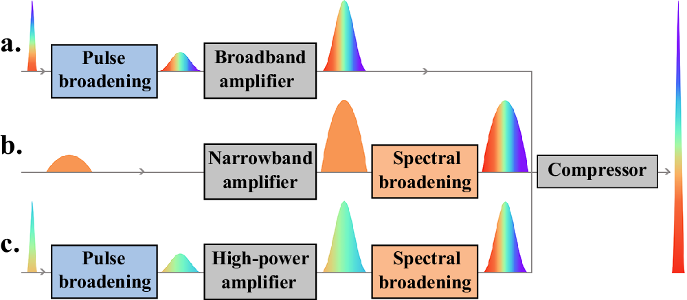
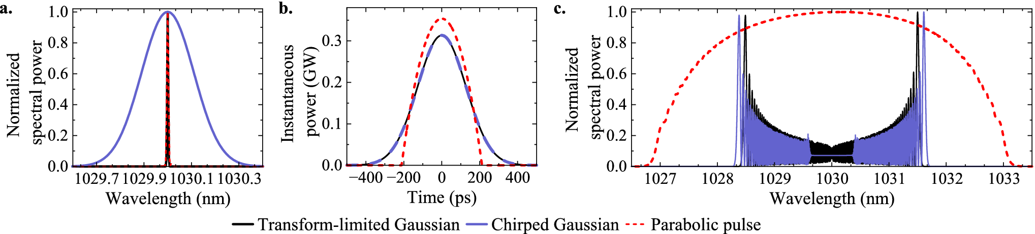

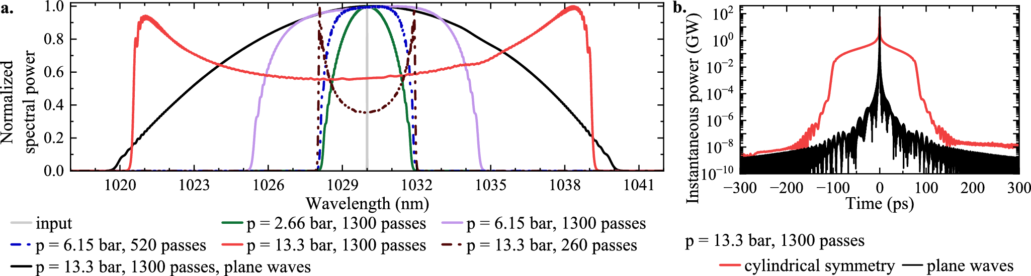


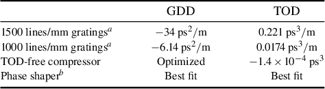
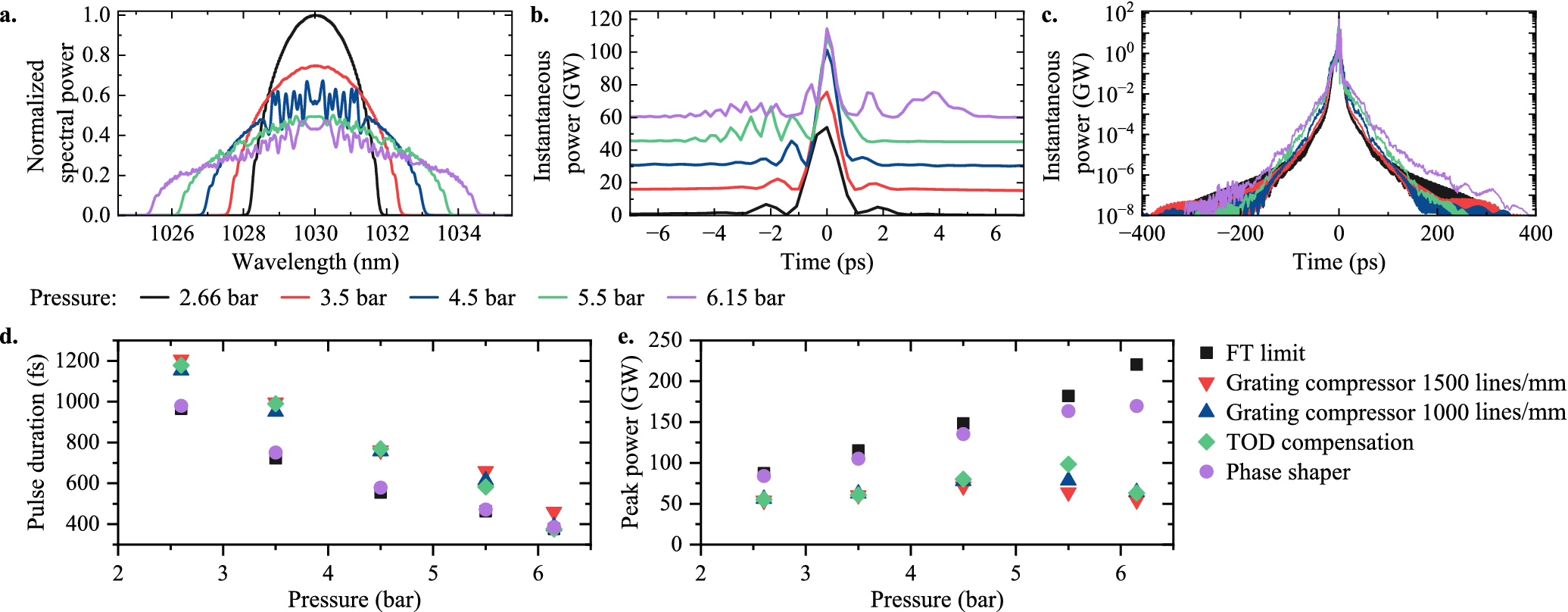
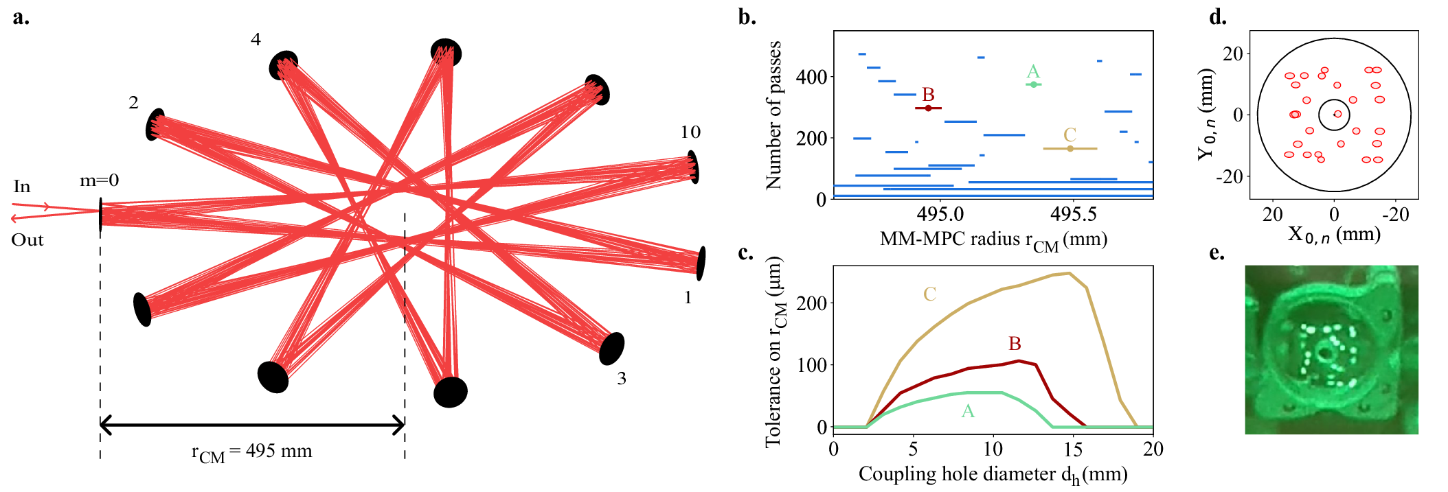


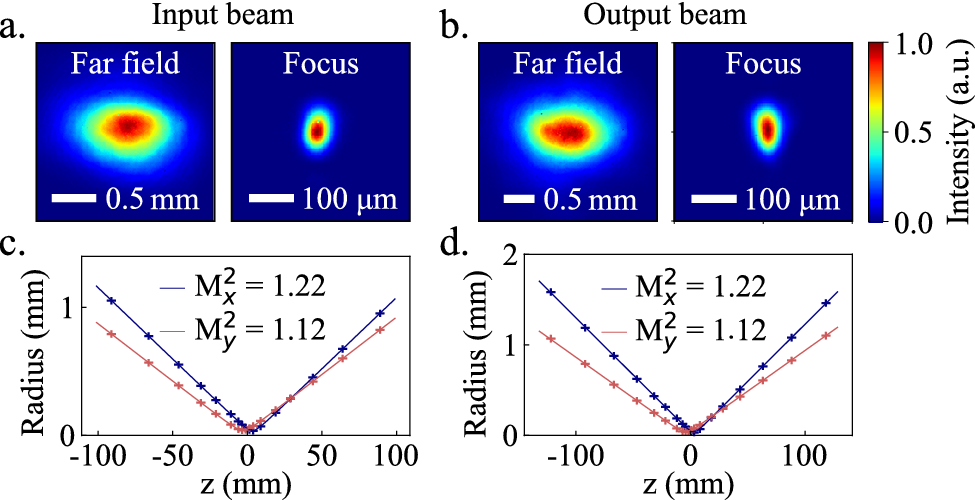


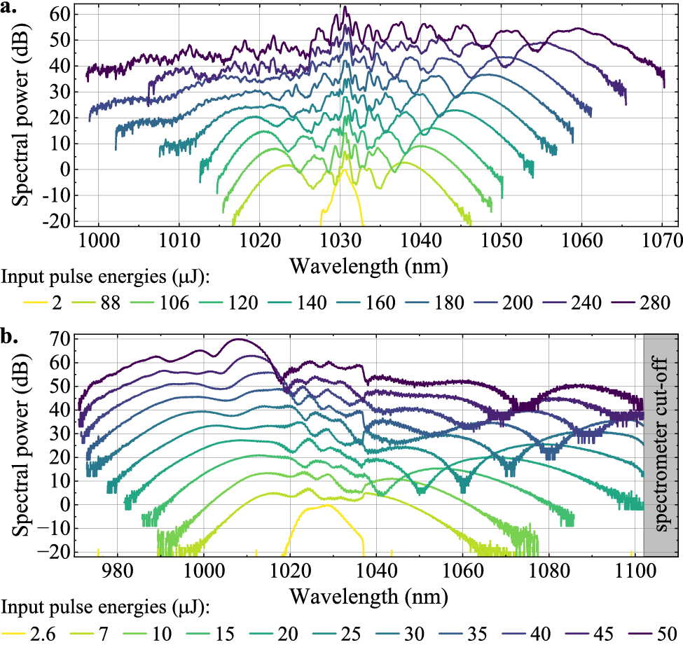
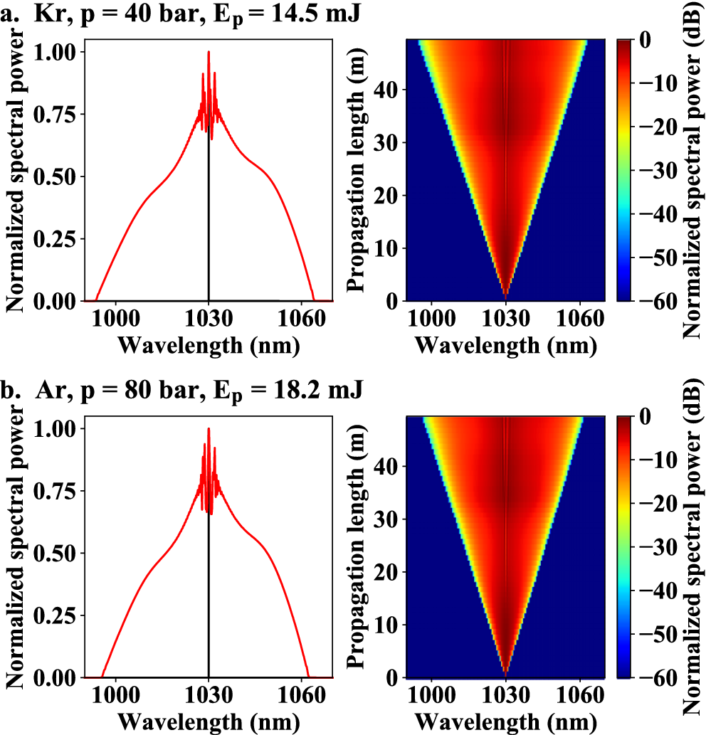
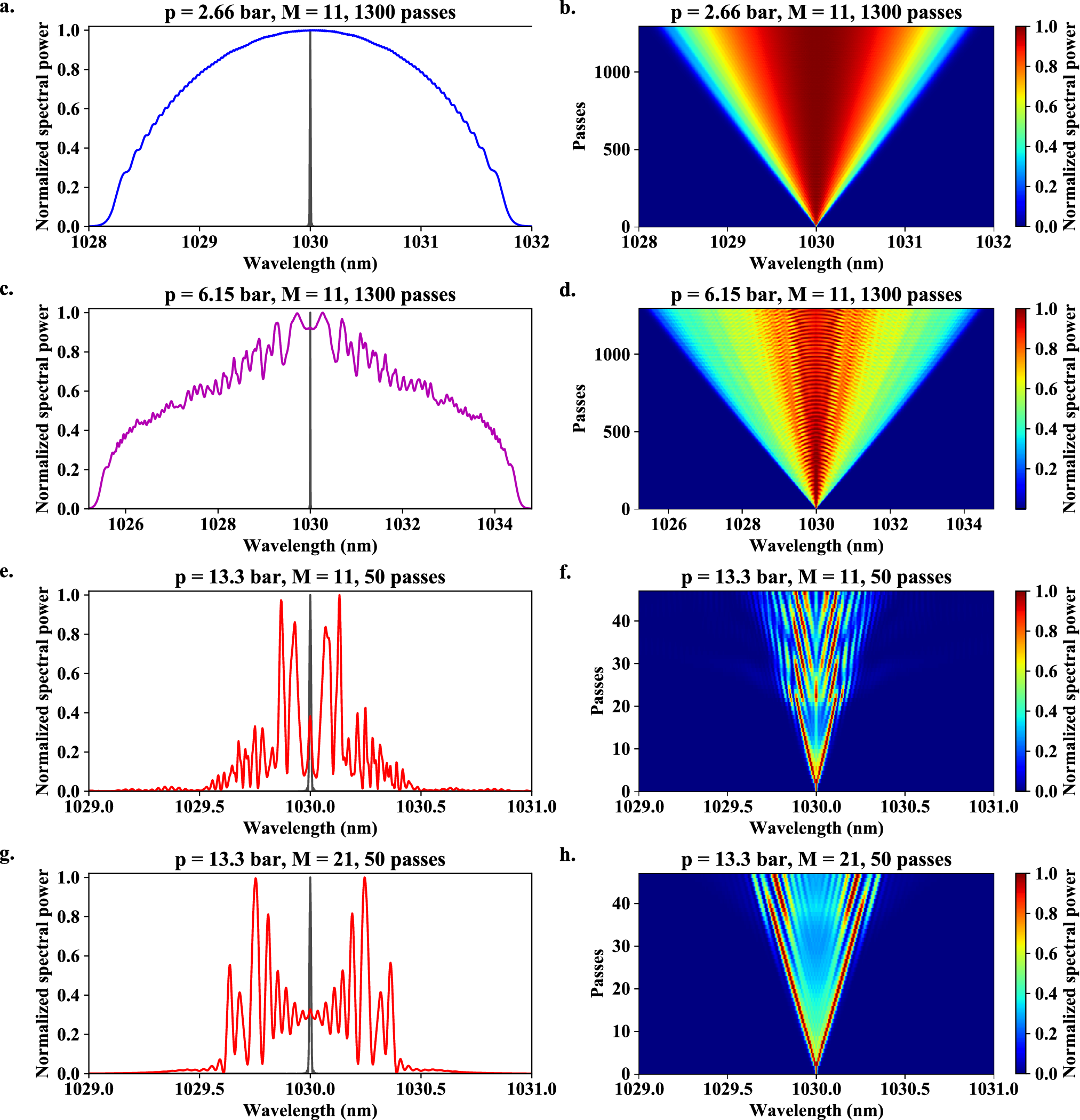


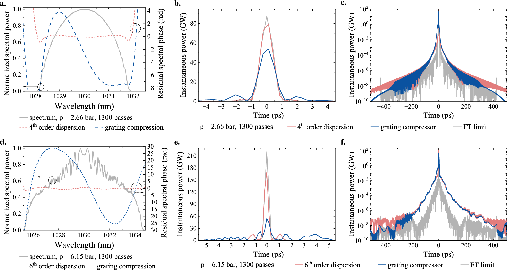


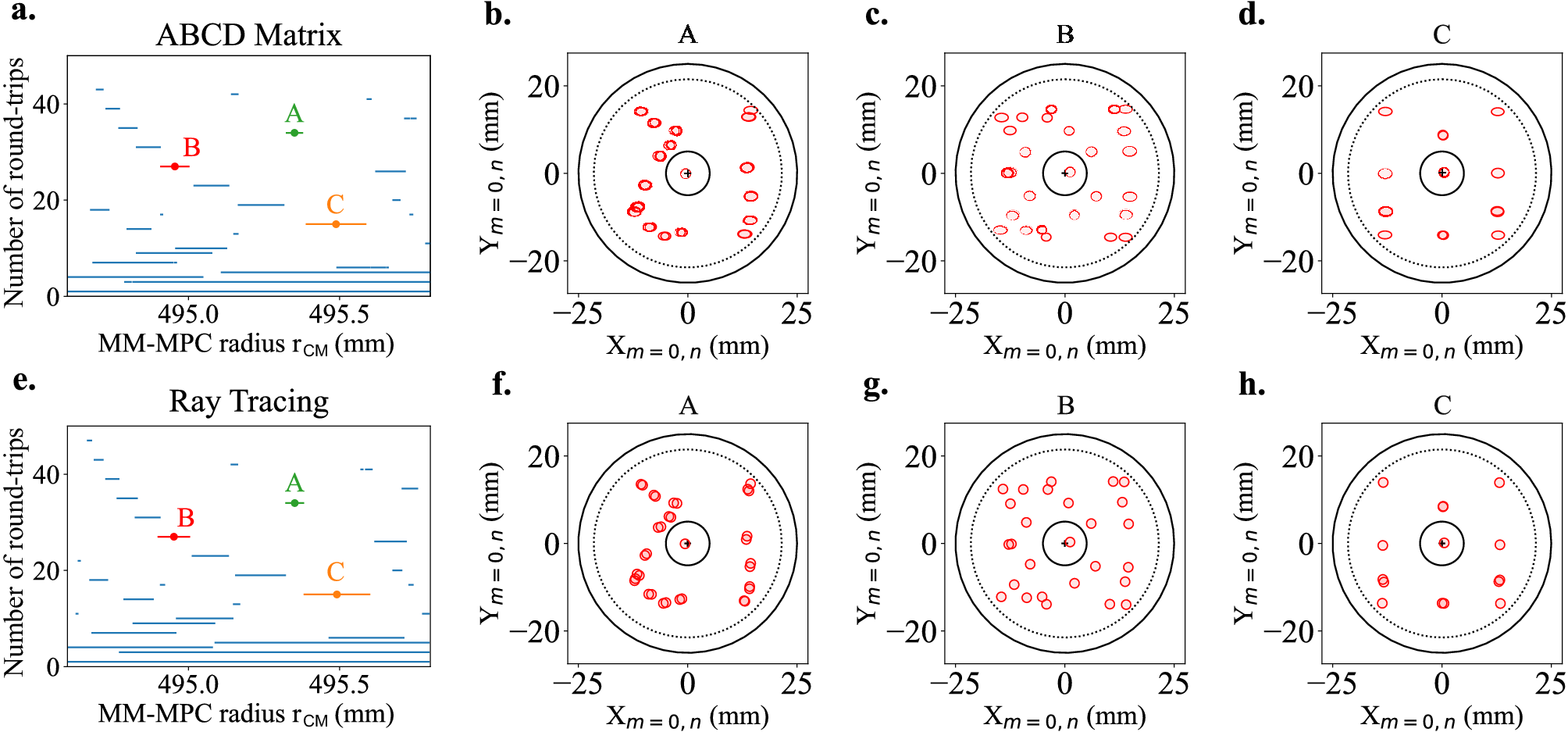


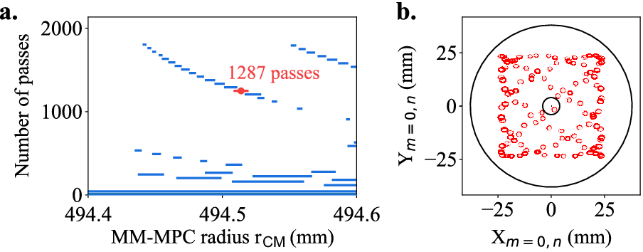


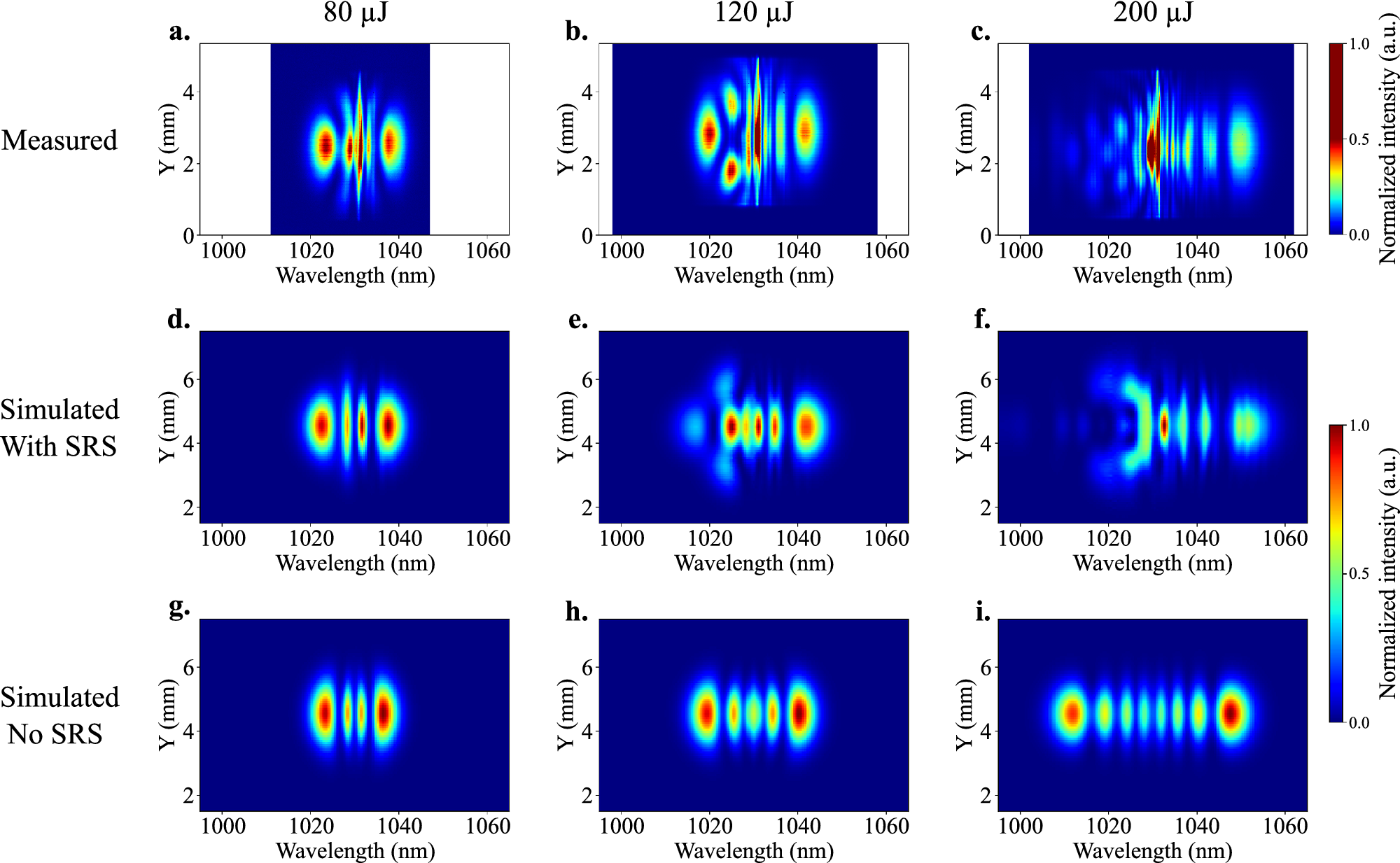




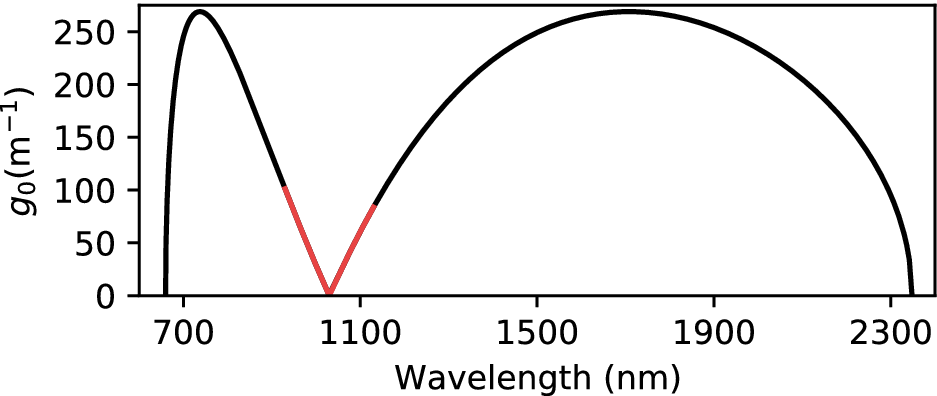


 Open access

