1. Introduction
Low-to-moderate Reynolds number flow is of interest in connection with a variety of engineering applications including the design of unmanned aerial vehicles, rotor and propeller blades, cooling fans and small wind turbines. Therefore, this phenomenon has regained interest in recent years (Desquesnes, Terracol & Sagaut Reference Desquesnes, Terracol and Sagaut2007; Sandberg et al. Reference Sandberg, Jones, Sandham and Joseph2009; Chong & Joseph Reference Chong and Joseph2012; Plogmann, Herrig & Würz Reference Plogmann, Herrig and Würz2013; Pröbsting, Serpieri & Scarano Reference Pröbsting, Serpieri and Scarano2014; Pröbsting, Scarano & Morris Reference Pröbsting, Scarano and Morris2015; Pröbsting & Yarusevych Reference Pröbsting and Yarusevych2015; Pröbsting et al. Reference Pröbsting, Zamponi, Ronconi, Guan, Morris and Scarano2016; Arcondoulis et al. Reference Arcondoulis, Doolan, Zander, Brooks and Liu2019a; Sanjose et al. Reference Sanjose, Towne, Jaiswal, Moreau, Lele and Mann2019; Ricciardi, Arias-Ramirez & Wolf Reference Ricciardi, Arias-Ramirez and Wolf2020; Yakhina et al. Reference Yakhina, Roger, Moreau, Nguyen and Golubev2020; Golubev Reference Golubev2021). Tonal noise emission has been extensively reported for flow conditions with the chord-based Reynolds number  $5\times 10^{4}< Re<2\times 10^{6}$ and the angle of attack
 $|\alpha |<10^{\circ }$ on symmetric aerofoils, e.g. NACA 0006, NACA 0008 (Sandberg et al. Reference Sandberg, Jones, Sandham and Joseph2009), NACA 0012 (Paterson et al. Reference Paterson, Vogt, Fink and Munch1973; Desquesnes et al. Reference Desquesnes, Terracol and Sagaut2007; Jones & Sandberg Reference Jones and Sandberg2011; Pröbsting et al. Reference Pröbsting, Scarano and Morris2015; Stalnov, Chaitanya & Joseph Reference Stalnov, Chaitanya and Joseph2016; Golubev Reference Golubev2021; Nguyen et al. Reference Nguyen, Golubev, Mankbadi, Yakhina and Roger2021) and NACA 0018 (Paterson et al. Reference Paterson, Vogt, Fink and Munch1973; Nakano, Fujisawa & Lee Reference Nakano, Fujisawa and Lee2006). Cambered aerofoils designed for small wind turbines and fan blades were also reported to generate tonal noise in the Reynolds number range of
 $5\times 10^{4}$–
 $6\times 10^{5}$ and light loading conditions (Longhouse Reference Longhouse1977; Oerlemans Reference Oerlemans2003; Wang et al. Reference Wang, Moreau, Iaccarino and Roger2009; Sanjose et al. Reference Sanjose, Towne, Jaiswal, Moreau, Lele and Mann2019; Yakhina et al. Reference Yakhina, Roger, Moreau, Nguyen and Golubev2020).
An early survey of aerofoil tonal noise was presented by Paterson et al. (Reference Paterson, Vogt, Fink and Munch1973) through experimental tests on a NACA 0012 aerofoil for the Reynolds number range  $8\times 10^{5}$–
 $2.2\times 10^{6}$, corresponding to full-scale helicopter rotors. While one dominant tone was noticed for most tested free-stream velocities, two dominant tones were observed at intermediate velocities, marking a frequency ‘jump’ (Paterson et al. Reference Paterson, Vogt, Fink and Munch1973). The resulting scatter plot of velocity against the frequency of the dominant tone showed a ladder-type structure, where the ‘jumps’ form the rungs of the ladder. In between the ‘jump’, the frequency of the dominant tone varies continuously with
 $u_\infty ^{0.8}$, where
 $u_\infty$ is the free-stream velocity. The ladder-type structure results in an overall scaling of the dominant tone frequency with approximately
 $u_\infty ^{1.5}$. Paterson et al. (Reference Paterson, Vogt, Fink and Munch1973) suggested that the underlying mechanism was similar to the shedding in the wake of a bluff body. A different explanation involving an acoustic feedback-loop (AFL) concept was later suggested (Tam Reference Tam1974). The AFL model proposed that the instability of the upstream boundary layer induced a sufficiently strong, lateral vibration in some highly localised region of the wake, which acted as a noise source. The acoustic waves in turn fed back upstream to sustain the oscillation of the boundary layer. Therefore, the noise source region in the wake and an upstream receptivity point, which Tam (Reference Tam1974) suggested to be located close to the trailing edge (TE), formed a feedback loop. The phase condition necessary for the existence of such an AFL was consistent with the existence of several distinct frequencies at a given velocity. The AFL model has since been widely accepted for providing both the sufficient and necessary conditions for aerofoil tonal noise.
Modifications to the AFL model of Tam (Reference Tam1974) were suggested later (see Fink Reference Fink1974; Longhouse Reference Longhouse1977; Arbey & Bataille Reference Arbey and Bataille1983; Chong & Joseph Reference Chong and Joseph2009; Arcondoulis et al. Reference Arcondoulis, Doolan, Zander, Brooks and Liu2019a). Instead of considering the AFL to occur in the wake, Longhouse (Reference Longhouse1977) hypothesised that the process actually begins far upstream on the aerofoil surface with the region of receptivity located near the leading edge. The receptivity point was also suggested to be near the maximum velocity point (Arbey & Bataille Reference Arbey and Bataille1983), the point at which the boundary layer instability was originated (Chong & Joseph Reference Chong and Joseph2009) or the separation point (Arcondoulis et al. Reference Arcondoulis, Doolan, Zander, Brooks and Liu2019a). In addition, for conditions at which vortices on both sides of the aerofoil possess similar strength near the TE, Desquesnes et al. (Reference Desquesnes, Terracol and Sagaut2007) and later Arcondoulis et al. (Reference Arcondoulis, Doolan, Zander, Brooks and Liu2019a) proposed a dual feedback mechanism to explain the side tones. Unlike the earlier AFL models (Tam Reference Tam1974; Arbey & Bataille Reference Arbey and Bataille1983), which proposed a phase condition for frequency selection of vortex shedding and tones, Desquesnes et al. (Reference Desquesnes, Terracol and Sagaut2007) explained the side tones by a bifurcation of symmetric and asymmetric vortex shedding from the suction and pressure sides. For a similar flow condition, Yang et al. (Reference Yang, Pröbsting, Liu, Zhang, Li and Li2021b) recently demonstrated the effect of dual vortex shedding on tonal noise generation experimentally, supporting the earlier findings of Desquesnes et al. (Reference Desquesnes, Terracol and Sagaut2007).
Pröbsting et al. (Reference Pröbsting, Scarano and Morris2015) identified several regimes for tonal noise generation on a NACA 0012 aerofoil at low-to-moderate Reynolds numbers: a regime dominated by pressure side events, one dominated by suction side events and an interaction regime, within which vortex shedding from both sides is relevant for noise generation. At high angles of attack and high Reynolds numbers, pressure side events dominate tonal noise generation, while at lower angles of attack and lower Reynolds numbers, suction side events become increasingly important. Later, Yang et al. (Reference Yang, Pröbsting, Liu, Zhang, Li and Li2021b) showed experimentally that modulation of the main tone within the interaction regime can be related to the phase difference of the vortex shedding process from the two sides of the aerofoil's TE. Small differences in the shedding frequency on both sides of the aerofoil result in varying in- and out-of-phase shedding, and thus modulation of the amplitude of the main tone. However, this type of modulation mechanism is not possible for flow conditions, where events on a single side of the aerofoil dominate tonal noise generation.
Along with the controversies surrounding AFL models and modulation mechanisms, the acoustic spectra reported in the literature also show distinct differences. The acoustic spectra observed by Paterson et al. (Reference Paterson, Vogt, Fink and Munch1973) for a NACA 0012 aerofoil at  $\alpha = 6^{\circ }$ and
 $Re = 8\times 10^{5}$ featured by narrowband energy content resembling tonal noise. Arbey & Bataille (Reference Arbey and Bataille1983) performed tests on a NACA 0012 aerofoil at
 $\alpha = 0^{\circ }$ and
 $u_\infty = 20\unicode{x2013}40\,{\rm m}\,{\rm s}^{-1}$ in an open-jet wind tunnel. They observed multiple equidistantly spaced, discrete tones superimposed on a broadband hump. Noise emission was dominated by one single tone at low Reynolds numbers, while it comprised multiple tones of comparable amplitude at higher Reynolds numbers (Arbey & Bataille Reference Arbey and Bataille1983). Yakhina et al. (Reference Yakhina, Roger, Moreau, Nguyen and Golubev2020) categorised tonal noise emission in several regimes: a switching regime between two tones that are not observed simultaneously, a regime with one or two tones and a regime with multiple unstable tones. Therefore, the basic characteristics of the acoustic spectra have been described in the literature, while the respective flow fields and underlying aeroacoustics mechanisms resulting in the different characteristics have not been fully understood yet. Furthermore, in the results shown by various authors, secondary side tones can be identified with smaller frequency intervals compared with the primary side tones (Arbey & Bataille Reference Arbey and Bataille1983; Desquesnes et al. Reference Desquesnes, Terracol and Sagaut2007; Pröbsting et al. Reference Pröbsting, Serpieri and Scarano2014, Reference Pröbsting, Scarano and Morris2015; Arcondoulis, Liu & Xu Reference Arcondoulis, Liu and Xu2019b). These secondary side tones can also be observed in numerical data at
 $\alpha = 2^{\circ }$,
 $Re = 2\times 10^{5}$ (Desquesnes et al. Reference Desquesnes, Terracol and Sagaut2007) and at
 $\alpha = 0^{\circ }$,
 $Re = 1\times 10^{5}$ (Ricciardi et al. Reference Ricciardi, Arias-Ramirez and Wolf2020). As these tones appear for both experimental and numerical studies, the underlying mechanisms for these secondary side tones require a physical explanation.
Proper orthogonal decomposition (POD) analysis has proven to be an efficient tool for the data reduction of complex flow fields (Nakano et al. Reference Nakano, Fujisawa and Lee2006; Henning et al. Reference Henning, Kaepernick, Ehrenfried, Koop and Dillmann2008; Ribeiro & Wolf Reference Ribeiro and Wolf2017; Yang et al. Reference Yang, Pröbsting, Liu, Zhang, Li and Li2021b). Although the POD method has been applied for the analysis of the unsteady behaviour of a laminar separation bubble (LSB) (Lengani et al. Reference Lengani, Simoni, Ubaldi and Zunino2014; Ricciardi, Ribeiro & Wolf Reference Ricciardi, Ribeiro and Wolf2019), the temporal information of the modes has not been related to the far-field sound pressure data yet. The noise generating flow is defined by large scale, spanwise coherent flow structures (vortices) resulting from the roll-up of the separated shear layer. Traces of these large flow structures can be identified and characterised in a statistical sense using POD, which renders the method suitable for the analysis of aerofoil tonal noise. Henning et al. (Reference Henning, Kaepernick, Ehrenfried, Koop and Dillmann2008) conducted a correlation analysis between the POD temporal mode coefficients and the far-field sound pressure for cylinder wake flow. It was concluded that the most energetic modes make the largest contribution to the radiated sound. Yang et al. (Reference Yang, Pröbsting, Liu, Zhang, Li and Li2021b) found that the correlation between the temporal coefficients of the most energetic POD modes and sound pressure can greatly increase the signal-to-noise ratio by filtering out less coherent flow features when compared with the direct correlation between local velocity and sound pressure. Therefore, the temporal coefficients of the POD modes may support our understanding of the noise generation due to coherent flow structures.
In order to improve our understanding of the acoustic spectra and the underlying aeroacoustic mechanisms, synchronised particle image velocimetry (PIV) and noise measurements have been conducted. To assess the features of the flow contributing to the noise generation mechanism, the POD method is applied here to the flow field measurements. The experimental set-up is described in § 2. Section 3 discusses acoustic characteristics, before § 4 describes the time-average flow structure and § 5 the unsteady flow development. Finally, § 6 discusses modal decomposition of the flow field and its implication for the interpretation of the aeroacoustic source.
2. Experimental set-up and methodology
2.1. Wind tunnel and aerofoil model
Experiments were conducted in a low-speed, closed-loop, open-jet anechoic wind tunnel at Southern University of Science and Technology (SUSTech), as shown in figure 1. The tunnel has a rectangular test section with dimensions of  $0.6\,{\rm m} \times 0.55\,{\rm m}$. Its maximum free-stream velocity in the test section is
 $70\,{\rm m}\,{\rm s}^{-1}$. The flow enters the test section through seven screens, a honey comb and a
 $7:1$ contraction nozzle, which results in a turbulence intensity of less than 0.15 % at the maximum velocity. The inner dimensions of the anechoic chamber are
 $3.8\,{\rm m}\times 5.7\,{\rm m} \times 3.0\,{\rm m}$, with a cutoff frequency of 100 Hz and a free-field radius of 1.9 m. For further details of the aerodynamic performance and acoustic characteristics of the wind tunnel the reader may refer to Yang et al. (Reference Yang, Liu, Liu, Shen, Zhang, Wei, Liu and Xu2021a).
Experimental set-up of PIV (not drawn to scale). (a) Top view; (b) side view.

The aerofoil model had a span of 0.55 m and a chord length of 0.3 m. It was mounted vertically between two end plates. The upper end plate was made from acrylic glass, which allowed for optical access for the PIV camera. The inflow velocity was set at  $u_\infty = 11.2\unicode{x2013}33.8\,{\rm m}\,{\rm s}^{-1}$ (Reynolds number
 $2.0\times 10^{5}$–
 $7.0\times 10^{5}$) at
 $\alpha = 2^{\circ }$. The angle of attack was corrected according to the method described by Brooks, Marcolini & Pope (Reference Brooks, Marcolini and Pope1986). This results in flow conditions within the tonal noise generation regime (Pröbsting et al. Reference Pröbsting, Scarano and Morris2015). Tests at
 $u_\infty =10\unicode{x2013}25\,{\rm m}\,{\rm s}^{-1}$ (Reynolds number
 $2.0\times 10^{5}$–
 $5.1\times 10^{5}$) and
 $\alpha = 1^{\circ }$ were also conducted and the results are provided as supplements in Appendix A to confirm the trend of the primary and secondary types of frequency intervals for a wider range of flow conditions. The aerofoil model was made from acrylic glass with a polished surface finish, alleviating reflection of the laser light from the aerofoil surface and facilitating near-wall flow measurements. The aerofoil leading edge was 0.35 m downstream of the nozzle exit and its TE 0.2 m upstream of the end plate TE, as shown in figure 1.
2.2. PIV and acoustic measurements
Time-resolved planar PIV measurements were performed for the region around the TE, as shown in figure 1(a,b), which is generally accepted to constitute the sound source region (Golubev Reference Golubev2021). The field of view (FoV) (approximately  $3\times 3\,{\rm cm}^{2}$) covers the flow field on both the suction and pressure sides of the TE and is represented by a black rectangle in figure 1(a). The flow was seeded with dioctyl sebacate particles with a mean diameter of
 $1\, \mathrm {\mu }{\rm m}$. Illumination was provided by a Photonics Nd: YAG laser (50 mJ @ 1000 Hz), and the light sheet was directed from the aerofoil wake toward the leading edge, facilitating particle illumination on both sides of the aerofoil and preventing a shadowed region (Pröbsting et al. Reference Pröbsting, Scarano and Morris2015). A Phantom VEO410L (
 $1280\times 780$ pixels, 12 bit, pixel pitch
 $20\,\mathrm {\mu }{\rm m}$, maximum frame rate 5.2 kHz) equipped with a Nikon Micro-Nikkor 200 mm objective was used at a focal ratio of
 $f/4$, resulting in an optical magnification of approximately 0.8 for a distance of approximately 300 mm. Laser and cameras were synchronised using a LaVision Programmable Time Unit and operated using the LaVision DAVIS 10.0 software. Image pairs were acquired at a sampling frequency of 2.56 kHz, which is at least four times higher than the dominant acoustic tone frequency and therefore provides sufficient temporal resolution for the cases investigated here. The measurement duration was 2 s, providing a compromise between available camera memory capacity and the lowest frequency of interest (separation bubble oscillation). The PIV measurement was synchronised with sound pressure data acquisition for correlation analysis. Images were processed using an iterative multi-grid multi-pass technique with window deformation and a final window size of
 $16\times 16$ pixels. The overlap factor was 75 %, resulting in a vector spacing of 0.1 mm.
The far-field noise was measured by one Brüel & Kjær 4966-H-041 microphone with a sampling rate of 51 200 Hz for a duration of 20 s. It was positioned 1.5 m away from the aerofoil model and aligned with the aerofoil TE. An average periodogram method was used to generate estimates of the power spectrum density ( $\varPhi$, PSD). The number of samples per window was 12 800, resulting in a frequency resolution of 1.56 Hz. The Hanning window and an overlap of 50 % were applied in the analysis.
2.3. Uncertainty analysis
The bias error of PIV measurements mainly considers peak locking as a result of the large imaging aperture, which yields a diffraction spot smaller than the pixel diameter. This effect was mitigated by slightly defocusing the images (Raffel et al. Reference Raffel, Willert, Wereley and Kompenhans1998), adjusting the defocused particle image diameter to approximately 2 pixels. The procedure was validated by inspecting the histogram of particles image displacement (Wieneke Reference Wieneke2015), which showed no evidence of peak locking.
The random error in the PIV data was estimated by the image matching method introduced by Sciacchitano, Wieneke & Scarano (Reference Sciacchitano, Wieneke and Scarano2013), which includes contributions from random Gaussian noise, particle image size and density, in-plane and out-of-plane motion. The image matching method uses the measured velocity field to match the particle images of the recordings based on the processing algorithm (for example by window deformation or window shift). The approach detects particle images in each interrogation window. In the case of exact velocity measurements and very small  $\Delta t$, the displaced particles in the first image match approximately those in the second image. In real experiments, the paired particle images do not match exactly and feature a positional disparity. The positional disparity is computed as the distance between the centroids of the particle images. The measurement uncertainty is determined within each interrogation window from the mean value and the statistical dispersion of the positional disparity vector. The uncertainty of the instantaneous velocity field is 1 % of the local velocity in the free-stream and 4 % in the boundary layer.
Following the estimation methods for convergence error of Fourier transform (Bendat & Piersol Reference Bendat and Piersol2010), the random error is analysed for the velocity and sound pressure spectrum. The random error is determined by the number of sub-blocks for averaging, and it depends on the window size, overlap and the recording time. The relative error for the magnitude of the power spectrum is  $1/\sqrt {n_d}$, where
 $n_d$ is the number of sub-blocks. The confidence interval with 68 % confidence level for sound pressure spectrum is [
 $-0.51$ dB, 0.46 dB], and that for the velocity spectrum is [
 $-1.76$ dB, 1.25 dB].
2.4. Proper orthogonal decomposition
POD analysis is a mathematical decomposition technique that determines a set of orthogonal basis functions for a set of input data. Basis functions constructed using this approach are optimal for reconstructing the original data (Berkooz, Holmes & Lumley Reference Berkooz, Holmes and Lumley1993). The extracted basis functions have been employed to identify dominant coherent flow features and to construct reduced-order flow models that capture the largest amount of energy with the smallest number of modes (Sirovich Reference Sirovich1987). There is extensive evidence that this decomposition tool is useful by reducing complexity and thus facilitating the understanding of flow mechanisms (van Oudheusden et al. Reference van Oudheusden, Scarano, van Hinsberg and Watt2005; Henning et al. Reference Henning, Kaepernick, Ehrenfried, Koop and Dillmann2008; Lengani et al. Reference Lengani, Simoni, Ubaldi and Zunino2014; Schrijer, Sciacchitano & Scarano Reference Schrijer, Sciacchitano and Scarano2014).
The results of the PIV measurements are a set of consecutive velocity fields, i.e. velocity components ( $U=[u,v]$), in the two-dimensional FoV
 $X = [x,y]$ as defined in figure 1(a). The fluctuating velocity component in the Reynolds decomposition is
 \begin{equation} U^{\prime}(X,t) = U(X,t) - \bar{U} (X,t), \end{equation}
where  $U(X,t)$ is the instantaneous,
 $\bar {U}(X,t)$ the time-averaged and
 $U^{\prime }(X,t)$ the fluctuating flow field. The proper decomposition is then applied on the auto-correlation matrix
 $C_{N_s\times N_s}$ as described by Sirovich (Reference Sirovich1987), Kourentis & Konstantinidis (Reference Kourentis and Konstantinidis2012), Schrijer et al. (Reference Schrijer, Sciacchitano and Scarano2014), Chen (Reference Chen2015) and Yang et al. (Reference Yang, Sciacchitano, Veldhuis and Eitelberg2016), which is defined as
 \begin{equation} C_{ij} = \frac{1}{N_s}\iint U^{\prime}(X,t_i) U^{\prime}(X,t_j)\,{\rm d}{X}, \end{equation}
where  $N_s$ is the number of snapshots. The integral is evaluated here as a summation of the discrete measurement points.
The eigenvalues  $\lambda _n$ and the eigenvectors
 $A_n(X)$ of the auto-correlation matrix satisfy
 \begin{equation} C_{{N_s\times N_s}}A_n(X) = \lambda_n A_n(X). \end{equation}
The POD mode, which represents the coherent flow pattern, is determined by
 \begin{equation} \varPsi_n(X) = \sum_{n=1}^{n=N_s} U^{\prime}(X,t_n) A_{n}(X). \end{equation}
Furthermore, the measurement data contain temporal information that can be retrieved by projecting each snapshot onto the basis functions
 \begin{equation} c_n(t) = \iint U^{\prime}(X,t_m) \varPsi_n(X) \,{\rm d}{X}, \end{equation}
where the coefficient  $c_n$ indicates the correlation between the
 $n$th basis POD spatial mode and the instantaneous flow field.
3. Characteristics of tonal noise
For the NACA 0012 aerofoil at  $\alpha = 2^{\circ }$ acoustic emission was measured in the velocity range 11.2–33.8
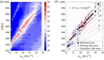
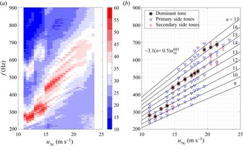
 ${\rm m}\,{\rm s}^{-1}$. Figure 2(a) shows a contour map of the acoustic spectra. The ladder-type structures can be identified clearly in form of the ridges (red). Figure 2(b) shows a scatter plot of the identified tones against velocity. The dominant tones are indicated by asterisks, primary side tones with large frequency intervals by triangles and secondary side tones with small frequency intervals by circles. These symbols will be shown and explained together with the sound pressure spectra in figure 3. The frequencies of the primary side tones
 $f_n^{(1)}$ (the superscript (1) represents the primary set of tones) can be fitted to the empirical relation of Arbey & Bataille (Reference Arbey and Bataille1983)
 \begin{equation} f_n^{(1)} = k \left(n+\frac{1}{2}\right) u_\infty^{0.85}, \end{equation}
where the value of  $k$ is determined to be 3.7 for a good fit, and the integers are indicated in figure 2(b) as
 $n = 7,\ldots,13$.
Variation of tonal noise with free-stream velocity. (a) Contour of acoustic spectra, and the contour level represents the PSD magnitude; (b) scatter plots of dominant (asterisks), primary side tones (triangles) and secondary side tones (circles). Here,  $\alpha = 2^{\circ }$.

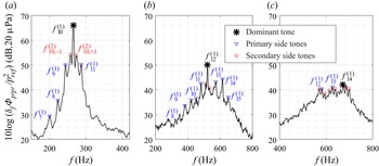
Acoustic spectra at different velocities. (a)  $12\,{\rm m}\,{\rm s}^{-1}$; (b)
 $18\,{\rm m}\,{\rm s}^{-1}$; (c)
 $21\,{\rm m}\,{\rm s}^{-1}$. Here,
 $\alpha = 2^{\circ }$. Primary (triangles) and secondary (circles) set of tones are indicated. Large asterisk indicates dominant tone.

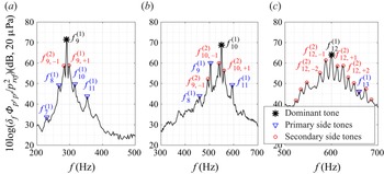
Figure 3(a–c) shows the acoustic spectra for velocities of  $u_\infty = 12, 18, 21\,{\rm m}\,{\rm s}^{-1}$. The spectra feature a broadband hump with superimposed tones (Arbey & Bataille Reference Arbey and Bataille1983; Chong & Joseph Reference Chong and Joseph2012). The dominant tone is marked by an asterisk in figure 3(a–c). The primary side tones, which follow the relation of Arbey & Bataille (Reference Arbey and Bataille1983), are indicated by triangles. This set of tones are described by the frequency selection criterion for the AFL (Arbey & Bataille Reference Arbey and Bataille1983). They are named as the primary set in this study and marked by
 $f_n^{(1)}$.
In addition to this first set of tones  $f_n^{(1)}$, figure 3 indicates a second set of tones
 $f_{n,i}^{(2)}$, which are referred to as secondary side tones in the remainder of this study and represented by circles in figure 3. They are distinctly different from the primary set as their frequency interval is 1/4–1/3 of the latter. In figure 3(a) for
 $u_\infty$ = 12
 ${\rm m}\,{\rm s}^{-1}$, this secondary set can be identified near the dominant tone
 $f_{9}^{(1)}$, and is represented by
 $f_{9,-1}^{(2)}$ and
 $f_{9,+1}^{(2)}$, respectively. In figure 3(b) for
 $u_\infty$ = 18
 ${\rm m}\,{\rm s}^{-1}$, it can be identified for both the dominant
 $f_{10}^{(1)}$ and for the first side tone
 $f_9^{(1)}$ of the primary set, which are represented as
 $f_{10,\pm 1}^{(2)}$ and
 $f_{9,-1}^{(2)}$, respectively. Different from the other cases, the secondary set provides the dominating tones at
 $21\,{\rm m}\,{\rm s}^{-1}$ in figure 3(c), and four strong tones of
 $f_{12,\pm 1}^{(2)}$ and
 $f_{12,\pm 2}^{(2)}$ are noted as examples.
The acoustic spectral shapes at the above three velocities show distinctive differences. At  $u_\infty = 12\,{\rm m}\,{\rm s}^{-1}$, a single tone is dominant in comparison with the other tones. The difference in the sound power between the dominant
 $f_9^{(1)}$ and the first side tone of the primary set
 $f_8^{(1)}$ exceeds 20 dB. At
 $u_\infty = 18\,{\rm m}\,{\rm s}^{-1}$, the first side tone of the primary set
 $f_9^{(1)}$ becomes comparatively stronger, and the difference in sound power of the dominant
 $f_{10}^{(1)}$ vs the first side tone
 $f_9^{(1)}$ of the primary set is less than
 $15$ dB. At
 $u_\infty = 21\,{\rm m}\,{\rm s}^{-1}$, multiple tones with comparable sound power emerge. For higher velocities, the spectra attain broadband characteristics and are not shown here. Therefore, the spectrum is characterised as progressively broadband in nature from
 $u_\infty = 12\,{\rm m}\,{\rm s}^{-1}$ to
 $u_\infty = 21\,{\rm m}\,{\rm s}^{-1}$.
Figure 4(a,b) shows the frequency intervals of the primary and secondary sets vs velocity, respectively. The frequency interval of the primary set vs flow velocity follows the power law of  $\Delta f_n^{(1)} = 3.7u_\infty ^ {0.85}$. The frequency interval of the secondary sets vs flow velocity follows the power law of
 $\Delta f_n^{(2)} = 0.6u_\infty$. The empirical function of frequency interval vs velocity was reported by Arbey & Bataille (Reference Arbey and Bataille1983) for a set of angles of attack, which is formulated as
 \begin{equation} L\Delta f = K u_\infty^{m}, \end{equation}
where  $L$ is the feedback-loop length, the empirical constant
 $K=0.89$ for similar conditions (Arbey & Bataille Reference Arbey and Bataille1983) and
 $m=0.85$ (see figure 2b). Applying this relation to the data for figure 4(a), the feedback-loop length is
 $L/c = 0.8$ for the primary set of tones. However, the calculated feedback-loop length for the secondary set according to (3.2) is
 $L/c=3.4$. This result should be noted and means that the feedback length scale must exceed the chord of the aerofoil. This is not possible and the selection of these frequencies cannot be explained by the feedback-loop model. Therefore, the secondary set of tones is different from the one discussed by Arbey & Bataille (Reference Arbey and Bataille1983) and others (e.g. Chong & Joseph Reference Chong and Joseph2012; Pröbsting et al. Reference Pröbsting, Scarano and Morris2015; Arcondoulis et al. Reference Arcondoulis, Doolan, Zander, Brooks and Liu2019a).
Frequency intervals of the primary (a) and secondary side tones (b).

The secondary set has not been identified as such before for various reasons. Paterson et al. (Reference Paterson, Vogt, Fink and Munch1973) analysed the acoustic spectra in third-octave bands. Also, narrow bands of approximately 10 Hz were used by Paterson et al. (Reference Paterson, Vogt, Fink and Munch1973) and Plogmann et al. (Reference Plogmann, Herrig and Würz2013). These frequency resolutions were insufficient to resolve the secondary side tones. The secondary set can, however, be identified in the experimental data shown by Arbey & Bataille (Reference Arbey and Bataille1983), Kingan & Pearse (Reference Kingan and Pearse2009), Chong & Joseph (Reference Chong and Joseph2013), Pröbsting et al. (Reference Pröbsting, Serpieri and Scarano2014) and Pröbsting et al. (Reference Pröbsting, Scarano and Morris2015), which adopted a frequency resolution in the range of 1–3 Hz. The secondary set can also be observed in numerical data at  $\alpha = 2^{\circ }$,
 $Re = 2\times 10^{5}$ in the study of Desquesnes et al. (Reference Desquesnes, Terracol and Sagaut2007) and
 $\alpha = 0^{\circ }$,
 $Re = 1\times 10^{5}$ in the study of Ricciardi et al. (Reference Ricciardi, Arias-Ramirez and Wolf2020). It should be mentioned that Desquesnes et al. (Reference Desquesnes, Terracol and Sagaut2007) showed acoustic spectra with frequency intervals of 1.84 Hz and 18.7 Hz, and the secondary side tones can only be observed for the smaller frequency interval of 1.84 Hz. However, the different nature of the secondary set tones with respect to the primary set tones was not discussed by these authors. Although the sound power of the tones of this set is generally lower than that of the dominant tone, it is often higher than that of tones in the primary side tone set, and it is also dominant over a restricted velocity range.
4. Flow separation on the pressure side
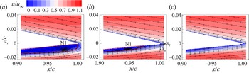
Figure 5(a–c) shows the time-averaged flow field with contours of the streamwise velocity component  $u$ for the three velocities, i.e.
 $u_\infty = 12$, 18 and
 $21\,{\rm m}\,{\rm s}^{-1}$. The wall-tangential and wall-normal coordinates are denoted by
 $x_t$ and
 $x_n$, respectively, as shown in figure 5(b). The flow fields feature LSBs, indicated by the solid lines (red) for
 $u_\infty = 12$ and
 $18\,{\rm m}\,{\rm s}^{-1}$. With increasing free-stream velocity or Reynolds number the reattachment point moves upstream. This is consistent with a shorter LSB length at higher Reynolds number as reported by e.g. Boutilier & Yarusevych (Reference Boutilier and Yarusevych2012) and Pröbsting & Yarusevych (Reference Pröbsting and Yarusevych2015). The existence of an LSB has been proposed earlier as a necessary condition for tonal noise generation (Nash, Lowson & McAlpine Reference Nash, Lowson and McAlpine1999; Desquesnes et al. Reference Desquesnes, Terracol and Sagaut2007), which is due to its amplification effect on the disturbances in the flow. At
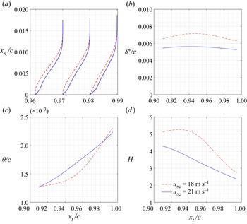
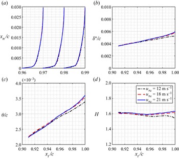
 $21\,{\rm m}\,{\rm s}^{-1}$, the LSB is not observed. This is attributed to the reduced bubble extent and height with increasing Reynolds number (Boutilier & Yarusevych Reference Boutilier and Yarusevych2012). In contrast, the flow on the suction side is fully attached to the aerofoil surface for all three flow conditions. The details of the boundary profiles, momentum thickness, displacement thickness and the shape factor on the pressure and suction sides for the three flow conditions are shown in Appendix B. Although the flow is attached on the suction side in the current FoV, it does not exclude the existence of an LSB in the upstream of the suction side.
Contours of time-averaged flow field coloured by the streamwise velocity component  $u$. The separation bubble is indicated by solid lines (red). N1 represents the streamwise position of the separation bubble's nodal point. The surface attached coordinate system
 $x_t$ and
 $x_n$ is indicated in (b) with the origin at the lower end of the TE: (a)
 $12\,{\rm m}\,{\rm s}^{-1}$; (b)
 $18\,{\rm m}\,{\rm s}^{-1}$; (c)
 $21\,{\rm m}\,{\rm s}^{-1}$.

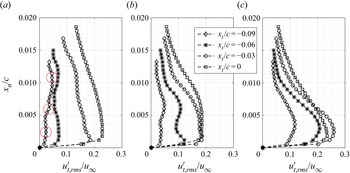
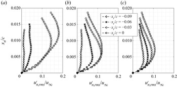
Figures 6 and 7, respectively, show significant streamwise and transverse velocity fluctuations in the boundary layer and near wake, which is characterised by root-mean-square (rms) value. The fluctuations of both velocity components on the pressure side are significantly higher than those on the suction side since the flow on the suction side is fully attached, whereas that on the pressure side is separated. Figure 8 shows the time-average velocity fluctuations  $u^{\prime }_{t,{rms}}$ at
 $x_t/c = -0.09, -0.06, -0.03$ and
 $0$. The values of
 $u_{t,{rms}}^{\prime }$ show evidence of three peaks, which are discernible at
 $x_t/c = -0.09$ for
 $u_\infty = 12\,{\rm m}\,{\rm s}^{-1}$ (red circles). This triple-peak structure of the streamwise velocity fluctuations is one of the features repeatedly reported for flow fields over aerofoils generating tones (Nash et al. Reference Nash, Lowson and McAlpine1999; Desquesnes et al. Reference Desquesnes, Terracol and Sagaut2007; Pröbsting et al. Reference Pröbsting, Serpieri and Scarano2014). Only double peaks and a single peak can be observed for
 $u_\infty = 18\,{\rm m}\,{\rm s}^{-1}$ and
 $21\,{\rm m}\,{\rm s}^{-1}$, respectively. A possible reason is that the reattachment point is located further upstream for this flow condition, and thus also the triple-peak structure can only be identified upstream of the FoV. Another possible explanation is that the aft portion of the separation bubble with the near-wall velocity fluctuations is not resolved in this case. Figure 9 shows the profiles of
 $u_{n,{rms}}^{\prime }$ for the three velocities. With a single peak in the measurement domain these profiles are similar to those reported by Desquesnes et al. (Reference Desquesnes, Terracol and Sagaut2007). The wall-normal velocity fluctuations show an increasing trend further downstream with Kelvin–Helmholtz (K–H) instability induced by vortex shedding, which will be elaborated on in the following section. The maximum values of
 $u^{\prime }_{n,{rms}}$ for all three velocities at the TE are attained at
 $x_n/c$ = 0.012, 0.0072 and 0.0072, respectively.
Contours of the root-mean-square value of  $u^{\prime }$: (a)
 $12\,{\rm m}\,{\rm s}^{-1}$; (b)
 $18\,{\rm m}\,{\rm s}^{-1}$; (c)
 $21\,{\rm m}\,{\rm s}^{-1}$.

Contours of the root-mean-square value of  $v^{\prime }$: (a)
 $12\,{\rm m}\,{\rm s}^{-1}$; (b)
 $18\,{\rm m}\,{\rm s}^{-1}$; (c)
 $21\,{\rm m}\,{\rm s}^{-1}$.

Profiles of  $u^{\prime }_{t,{rms}}$ along the wall-normal direction: (a)
 $12\,{\rm m}\,{\rm s}^{-1}$; (b)
 $18\,{\rm m}\,{\rm s}^{-1}$; (c)
 $21\,{\rm m}\,{\rm s}^{-1}$.

Profiles of  $u^{\prime }_{n,{rms}}$ along the wall-normal direction: (a)
 $12\,{\rm m}\,{\rm s}^{-1}$; (b)
 $18\,{\rm m}\,{\rm s}^{-1}$; (c)
 $21\,{\rm m}\,{\rm s}^{-1}$.

Figure 10(a,b) shows the evolution of the maximum velocity fluctuations over the boundary layer along the wall-tangential direction in terms of, respectively,  $u^{\prime }_{t,{rms}}$ and
 $u^{\prime }_{n,{rms}}$. The positive, linear slope indicates exponential growth for
 $u^{\prime }_{t,{rms}}$ (figure 10a) for
 $u_\infty = 12$ and
 $18\,{\rm m}\,{\rm s}^{-1}$ upstream of
 $x_t/c = -0.03$ and
 $-0.07$, respectively. This is a typical feature of the K–H instability (Ye, Schrijer & Scarano Reference Ye, Schrijer and Scarano2018). The regions of exponential growth coincide with the upstream part of the LSB (before the nodal point) as shown in figure 5. At
 $u_\infty = 21\,{\rm m}\,{\rm s}^{-1}$ the growth rate varies linearly with the tangential distance. The growth of
 $u^{\prime }_{n,{rms}}$ (figure 10b) shows trends similar to those for
 $u^{\prime }_{t,{rms}}$ discussed above. The velocity component of
 $u_n$ is regarded as the major component inducing wall pressure according to the theoretical considerations of Amiet (Reference Amiet1975), and thus it is chosen for further analysis of the noise source region.
Maximum value of velocity fluctuation along the wall-tangential direction: (a)  $u^{\prime }_{t,{rms}}$; (b)
 $u^{\prime }_{n,{rms}}$.

5. Vortex shedding over the separation bubble
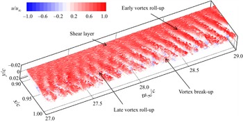
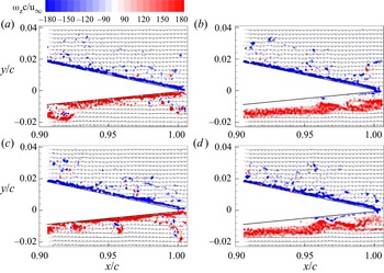
Figure 11 depicts a time sequence of spanwise vorticity  $\omega _z$ with colour contours of
 $u/u_\infty$. This time sequence of vorticity illustrates the temporal evolution of TE vortices, which can be identified as periodic, coherent streaks in the visualisation. Vorticity is concentrated in the shear layer in the upstream range. Vortex formation is observed in the range
 $0.9 < x/c < 0.95$ with the position varying over time. In the time range of
 $27< tu_\infty /c<28$ the vortex formation occurs late near the TE. For
 $28< tu_\infty /c<29$ vortex formation occurs further upstream. Near the TE, vortex break-up can also be observed.
Space–time development of the vortex structures visualised by the iso-surface of the spanwise vorticity.

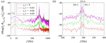
Figure 12 shows the PSD of the wall-normal velocity fluctuation  $u_n^{\prime }$ on the pressure side for
 $u_\infty = 12\,{\rm m}\,{\rm s}^{-1}$. The data were sampled at the wall-normal locations with maximum
 $u^{\prime }_{n,{rms}}$ in the boundary layer. The PSD was evaluated following the same method as applied for the sound pressure described above. The number of samples per window for estimating the PSD was set to 1280 with an overlap of 50 %, which results in a frequency resolution of 1.25 Hz. Mainly, two broadband humps are observed in figure 12(a): one is located in the low-frequency range centred at 7.5 Hz, and the other one centred around 293.8 Hz. The tones near the second hump are shown in an enlarged view in figure 12(b). The set of discrete tones are 286.3 Hz, 293.8 Hz and 301.3 Hz, corresponding to a frequency interval of 7.5 Hz. This frequency interval matches the centre frequency of the low-frequency broadband hump indicated in figure 12(a) (vertical dashed line). The amplitude associated with the maximum peak has an increasing trend in the downstream direction. In addition, the narrowband characteristics of the sound pressure and velocity spectra agree well (compare figures 3b and 12a).
Spectra of  $u_n^{\prime }$ on the pressure side,
 $u_\infty = 12 \,{\rm m}\,{\rm s}^{-1}$. (a) Global view; (b) detail view.

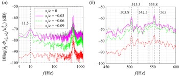
The spectra of wall-normal velocity fluctuation  $u_n^{\prime }$ on the pressure side are shown in figure 13 for
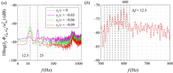
 $u_\infty = 18\,{\rm m}\,{\rm s}^{-1}$. The low-frequency oscillation is centred at 11.5 Hz, while the high-frequency discrete tones are centred around 503.8 Hz and 553.8 Hz, which correspond to the primary side tones, as shown in figure 3. The secondary side tones have a frequency of 515.3 Hz (with the centre of 503.8 Hz), 542.5 and 565 Hz (with the centre of 553.8 Hz), as shown in figure 13(b), resulting in a frequency interval of 11.5 Hz, which corresponds to the centre frequency of the low-frequency broadband hump in figure 13(a). Figure 14 shows the spectra of velocity fluctuation
 $u_n^{\prime }$ for
 $u_\infty = 21\,{\rm m}\,{\rm s}^{-1}$. Here, the low-frequency oscillation is centred at 12.5 Hz and its harmonic of 25 Hz. The high-frequency discrete tones are equidistantly spaced with an interval of 12.5 Hz.
Spectra of  $u_n^{\prime }$ on the pressure side,
 $u_\infty = 18\,{\rm m}\,{\rm s}^{-1}$. (a) Global view; (b) detail view.

Spectra of  $u_n^{\prime }$ on the pressure side,
 $u_\infty = 21 \,{\rm m}\,{\rm s}^{-1}$. (a) Global view; (b) detail view.

Figure 15 shows the spectra of wall-normal velocity fluctuation  $u_n^{\prime }$ on the suction side for
 $u_\infty = 18\,{\rm m}\,{\rm s}^{-1}$. The spectra are predominantly of broadband character. This is an indication of tonal noise generation being dominated by events on the pressure side exclusively (Pröbsting et al. Reference Pröbsting, Scarano and Morris2015). Similar broadband spectra of vertical velocity fluctuations are also observed for the cases of
 $u_\infty = 12\,{\rm m}\,{\rm s}^{-1}$ and
 $21\,{\rm m}\,{\rm s}^{-1}$, which have been omitted here for brevity. Pressure side dominated cases at high Reynolds numbers were observed and characterised as such by Pröbsting et al. (Reference Pröbsting, Scarano and Morris2015). For a NACA 0012 at
 $\alpha = 2^{\circ }$ noise generation was described as suction side dominated for Reynolds numbers below
 $2\times 10^{5}$ and as pressure side dominated for the Reynolds numbers between
 $2\times 10^{5}$ and
 $1\times 10^{6}$ (Pröbsting et al. Reference Pröbsting, Scarano and Morris2015). In the present study with
 $\alpha = 2^{\circ }$ and the Reynolds number range of
 $2.5\times 10^{5}$–
 $7.2\times 10^{5}$, the dominance of pressure side events for tonal noise generation is consistent with this description. In addition, there is notably no clear broadband hump in the low-frequency range around 11.5 Hz on the suction side, which was observed on the pressure side (see figure 13a).
Spectra of  $u_n^{\prime }$ on the suction side;
 $u_\infty = 18 \,{\rm m}\,{\rm s}^{-1}$.

In order to identify the cause of the secondary modulation and thus an explanation for the frequency interval of the secondary side tones, various possibilities were considered. Firstly, acoustic resonance can be excluded since the selected frequencies of the secondary set continuously change with velocity and are thus not fixed as would be the case for a standing wave. Secondly, the frequencies related to the blade passing frequency of the wind-tunnel rotor  $O(10^{2})$ Hz in the current test range), which may introduce oscillations in the flow, are higher than the oscillation frequency observed here. Thirdly, the characteristic frequency for the flow passing through the wind-tunnel air loop (around 30 m) is of
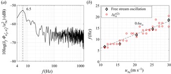
 $O(10^{-1})$ Hz, which is below the observed frequency as well. Finally, this leads to further investigation of the hydrodynamic fluctuations in the flow. To this end, PIV measurements on the empty wind tunnel were conducted. Velocity spectra in the empty test section of the facility are shown in figure 16(a) for
 $u_\infty = 11.2\,{\rm m}\,{\rm s}^{-1}$. A peak at 6.5 Hz is observed, roughly corresponding to a characteristic length of 1.7 m based on the free-stream velocity and approximately equal to the distance between the nozzle exit and collector (1.8 m for this set-up). This length scale was identified previously as the feedback-loop length for low-frequency oscillations in open-jet wind tunnels (Rockwell & Naudascher Reference Rockwell and Naudascher1979). The peak frequency vs free-stream velocity in the empty wind tunnel is shown in figure 16(b). The scattered data suggest a linear fit of 0.6
 $u_\infty$ and which agrees well with the frequency interval of the secondary side tones as shown in figure 4(b). This low-frequency oscillation has been observed for many open-jet wind tunnels. A list of the wind tunnels can be found in Jin et al. (Reference Jin, Sun, Jiang, Liang and Zhang2021).
(a) Velocity spectra at the model centre of the empty wind tunnel,  $u_\infty = 11.2\,{\rm m}\,{\rm s}^{-1}$; (b) Frequency of oscillation peak vs free-stream velocity for the empty wind tunnel (the frequency intervals of the secondary side tones are also plotted here for the purpose of comparison).

The low-frequency oscillation can be observed in the empty wind tunnel, as shown in figure 16, yet its impact on the suction side is negligible for the turbulent flow near the TE as shown in figure 15. The oscillations are amplified through the separation bubble on the pressure side as suggested by Yarusevych & Kotsonis (Reference Yarusevych and Kotsonis2017). This is in agreement with studies employing forced disturbances, in which only the LSB was receptive to the external excitation (Marxen, Lang & Rist Reference Marxen, Lang and Rist2013; Yarusevych & Kotsonis Reference Yarusevych and Kotsonis2017; Kurelek, Kotsonis & Yarusevych Reference Kurelek, Kotsonis and Yarusevych2018; Pröbsting & Yarusevych Reference Pröbsting and Yarusevych2021).
In addition, the low-frequency oscillation for the flow with an LSB was not only observed in experimental studies, but also in many numerical studies (e.g. Alam & Sandham Reference Alam and Sandham2000; Spalart & Strelets Reference Spalart and Strelets2000; Wissink & Rodi Reference Wissink and Rodi2002, Reference Wissink and Rodi2003, Reference Wissink and Rodi2004; Jones, Sandberg & Sandham Reference Jones, Sandberg and Sandham2008; Yakhina et al. Reference Yakhina, Roger, Moreau, Nguyen and Golubev2020), where it is typically called the ‘wavering’ mode (Spalart & Strelets Reference Spalart and Strelets2000; Wissink & Rodi Reference Wissink and Rodi2004). As there are no facility effects in numerical simulations, unless the facility is explicitly modelled, there must be another cause. Wissink & Rodi (Reference Wissink and Rodi2004) suggested that the fluctuation of an LSB was introduced at the inlet by making use of the cyclic ‘isotropic’ turbulence from a separate simulation in a cubic box. The size of the box determines the disturbance frequency at the inlet. Other disturbances during the simulations of LSB were triggered by introducing disturbances into the boundary layer (Alam & Sandham Reference Alam and Sandham2000; Maucher et al. Reference Maucher, Rist, Kloker and Wagner2000), by round-off error (Spalart & Strelets Reference Spalart and Strelets2000; Wissink & Rodi Reference Wissink and Rodi2002) or by oscillations in the outlet flow (Wissink & Rodi Reference Wissink and Rodi2003). Instead of external disturbances, a self-sustained perturbation mechanism was suggested by Jones et al. (Reference Jones, Sandberg and Sandham2008), and the two-dimensional vortex shedding behaviour was found to be absolutely unstable to three-dimensional perturbations. The instability was associated with the production of streamwise vortices located in the braid region between successive spanwise vortices (Jones et al. Reference Jones, Sandberg and Sandham2008), with a similar mechanism to that of mode-B instability as observed in bluff-body wakes (Williamson Reference Williamson1996).
6. Relation between the flow structures and tones
For the acoustic spectra (Section 3) two sets of side tones were identified with the associated frequencies matching peaks observed in the velocity spectra in § 5. One case with a single dominant tone ( $12\,{\rm m}\,{\rm s}^{-1}$), one case with comparable primary and secondary side tones (
 $18\,{\rm m}\,{\rm s}^{-1}$) and a third case characterised by the dominating secondary side tone set (
 $21\,{\rm m}\,{\rm s}^{-1}$) were identified and selected in the low, moderate and high velocity ranges, respectively. To identify the most energetic fluctuations as well as their contributions to the peaks in the velocity spectra, the coherent structures in the flow are analysed for these three cases using POD.
6.1. Condition with a single dominant tone
6.1.1. POD modes
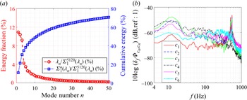
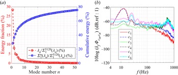
For  $u_\infty = 12\,{\rm m}\,{\rm s}^{-1}$, all 5120 snapshots were used for the POD analysis following the procedure described in § 2.4. The energy fraction of each mode (red circle) is indicated by the left
 $y$-axis of figure 17(a) and the cumulative energy (blue square) indicated by the right
 $y$-axis. Herein, the contribution of the first 50 modes to the turbulent kinetic energy (TKE) is
 $76\,\%$ as demonstrated in figure 17(a). Similar to the POD analysis in the wake flow of a square-section cylinder (van Oudheusden et al. Reference van Oudheusden, Scarano, van Hinsberg and Watt2005) and jet flow (Kirby, Boris & Sirovich Reference Kirby, Boris and Sirovich1990), a large amount of energy is captured by a small number of modes. The first and second modes account for 17.4 % and 15.5 % of the TKE, respectively, which are higher than the other modes, as shown in figure 17(a).
(a) Energy distribution of the POD modes; (b) frequency spectra of the mode time coefficients  $c_n$. Here,
 $u_\infty = 12\,{\rm m}\,{\rm s}^{-1}$.

The POD mode time coefficients as defined in (2.5) allow for the phase identification of instantaneous flow fields resulting from a projection on a specific mode, which is similar to those described in van Oudheusden et al. (Reference van Oudheusden, Scarano, van Hinsberg and Watt2005) and Lengani et al. (Reference Lengani, Simoni, Ubaldi and Zunino2014). The spectra of  $c_n$ for low-order POD modes are shown in figure 17 and have been obtained using the parameters also used in the estimation of the PSD for
 $u^{\prime }_{n}$ with a frequency resolution of 1.25 Hz. The spectral shapes of modes 1–6 are similar and show broadband humps around 7.5 Hz and 292.5 Hz, respectively, which capture the main features of the velocity fluctuations. The modes with the highest peak at the dominant tone frequency are modes 1 and 2. Mode 3 features its highest peak at a frequency of 7.5 Hz. Higher-order modes with lower TKE are not shown here for brevity.
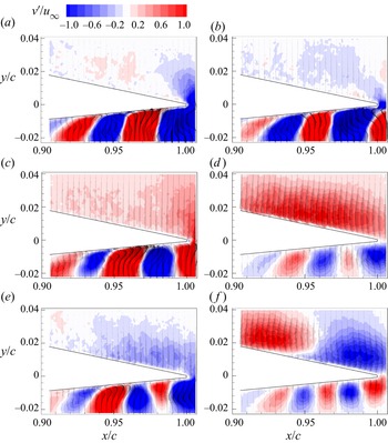
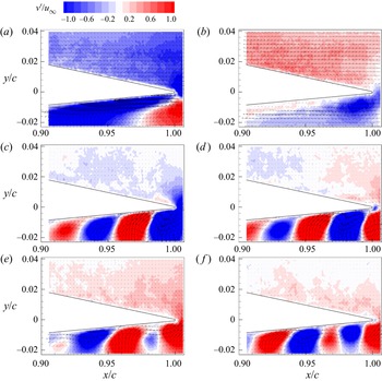
Figure 18 visualises the dominant modal features by depicting the first six POD modes. The corresponding time-averaged flow field, typically called the zeroth mode (stationary component), is shown in figure 5(a). In figure 18 velocity vectors are superimposed on contours of  $v^{\prime }$. Alternating coherent regions of positive and negative velocity fluctuations are observed on the pressure side. The wavelength of the velocity pattern has an increasing trend towards TE. A pair of POD modes are expected with a phase shift of
 ${\rm \pi} /2$ to describe convection behaviour, which is in line with the results presented here (van Oudheusden et al. Reference van Oudheusden, Scarano, van Hinsberg and Watt2005; Lengani et al. Reference Lengani, Simoni, Ubaldi and Zunino2014). Indeed, modes 1 and 2 (figure 18a,b) are orthogonal, as expected for coupled POD modes. Modes 3 and 4 also show coherent velocity fluctuations, yet the fluctuation content is concentrated near the rear part of the aerofoil. For modes 5 and 6 the periodic flow features are found on both the pressure and suction sides, with the suction side wavelength considerably larger than that seen on the pressure side.
The flow structures corresponding to the first to sixth modes (a–f). Here,  $u_\infty = 12\,{\rm m}\,{\rm s}^{-1}$.

6.1.2. Sound pressure fluctuation: contributions from the POD modes
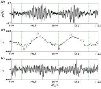
Figure 19(a) shows the filtered sound pressure signal with a cutoff frequency 100 Hz ( $limit$ of the anechoic chamber). The time history of the filtered sound pressure is characterised by high-frequency oscillations with small-amplitude modulation, as expected from the sound pressure spectra at
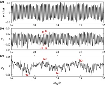
 $u_\infty = 12\,{\rm m}\,{\rm s}^{-1}$ (see figure 3b). In order to find the contributions of the coherent flow structures to sound generation, the time histories of the dominant POD mode time coefficients
 $c_n$ are presented in figure 19(b,c). A comparison between the time histories of the POD mode coefficients and the sound pressure can help identify the contributions of the flow patterns to different sound pressure signatures.
Time histories of sound pressure and POD mode time coefficients. (a) Sound pressure; (b) POD mode coefficient  $c_1$; (c)
 $c_3$. J1–J4 represent instants with large amplitudes of
 $c_1$, and K1–K4 represent instants with large envelope amplitudes of
 $c_3$. Here,
 $u_\infty = 12\,{\rm m}\,{\rm s}^{-1}$.

The time axis is aligned between  $p^{\prime }$ and
 $c_n$ by correcting for the retarded time due to sound propagation from the source to the receiver. Such an alignment of the time axis is justified for the following reasons. Firstly, the noise source is assumed to be located at the TE, which is generally accepted for the flow conditions discussed here (Arbey & Bataille Reference Arbey and Bataille1983; Desquesnes et al. Reference Desquesnes, Terracol and Sagaut2007; Pröbsting et al. Reference Pröbsting, Serpieri and Scarano2014; Golubev Reference Golubev2021). Secondly, the noise source is quasi two-dimensional and the coherence length of the flow along the span is approximately 1.5 times the span of the aerofoil model (a stereo PIV test in the spanwise-vertical plane was performed yet the result is not shown here for brevity) at
 $u_\infty = 12\,{\rm m}\,{\rm s}^{-1}$. Thirdly, the difference in retarded time from the mid-span and tip points, respectively, to the microphone is
 $72\,\mathrm {\mu }{\rm s}$, which corresponds to a frequency of approximately 13.7 kHz. This exceeds the maximum frequency of interest (600 Hz) by a factor of approximately 23, and can be considered to be negligible for the analysis here. Therefore, the retarded time calculation is based on the sound wave travelling time between the mid-span location of the TE and the microphone position. As the time coefficient of the second mode has a similar spectral shape with respect to the first mode (see figure 17b), and higher modes already possess lower turbulent kinetic energy (see figure 17a), only the time histories of
 $c_1$ and
 $c_3$ are shown here for brevity. By comparing the time history of
 $p^{\prime }$ with those of
 $c_1$ and
 $c_3$, it is found that the high-frequency oscillation of
 $c_1$ is consistent with that of
 $p^{\prime }$. Other than the high-frequency oscillation, the time histories of
 $c_3$ also show a low frequency oscillation at approximately 7.5 Hz and its harmonics.
The marked symbols of J1–J4 indicate consecutive minima and maxima of the high-frequency fluctuation of  $c_1$, which relate to the main tone at frequency
 $f_{n}^{(1)} = 293$ Hz of
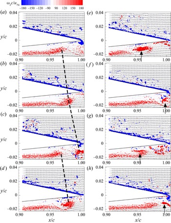
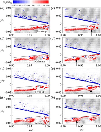
 $p^{\prime }$. The flow fields at these instants are displayed in figure 20. For instant J1, the instantaneous flow field, corresponding to a local minimum of
 $c_1$, is shown in figure 20(a). Shear layers with concentrated vorticity are visible on both sides near the TE. On the pressure side this shear layer is separated from the surface of the aerofoil and rolls up to form a vortex near the TE. Half the period of the main tone later, at instant J2, the value of
 $c_1$ attains a local maximum. The corresponding instantaneous flow field is shown in figure 20(b). With respect to J1 the discrete vortices have an obvious displacement in the streamwise direction. Another semi-period of the main tone frequency later, at instant J3, the value of
 $c_1$ attains another local maximum. The corresponding flow field in figure 20(c) appears similar to figure 20(a) at instant J1 in terms of vortex positions and phases. At instant J4, the shed vortex continues travelling downstream and looks similar to that at instant J2. Therefore, the first mode is ascribed to the periodic vortex shedding in the streamwise direction. This is consistent with the pattern of mode 1 as shown in figure 18(a). It is also noticed that the vortex roll-up occurs over a small range, i.e.
 $0.95 c$–
 $0.98 c$.
Flow fields of spanwise vorticity contours superimposed by velocity vectors for J1–J4 in (a–d) and for K1–K4 in (e–h) (see figure 19 for J1–J4 and K1–K4). The dashed lines represent the vortex convection in consecutive instants, and the arrows indicate the position of vortex roll-up. Here,  $u_\infty = 12\,{\rm m}\,{\rm s}^{-1}$.

The time history of  $c_3$ features a low-frequency oscillation at approximately 7–8 Hz, which is close to the frequency interval of secondary side tones. The examples for the flow fields at the instants with high values of
 $c_3$ amplitude envelope (K1–K4) in figure 20(e–h) help to explain the mechanism of secondary side tones in the acoustic spectra. These snapshots show a significant movement of the initiation of vortex roll-up (indicated by the arrows) on the separated shear layer. At instants K1 and K3 the vortex roll-up position starts at
 $0.96c$ while at instants K2 and K4 it moves downstream to
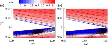
 $0.99 c$. Vortex roll-up occurs respectively close and far from TE inducing an amplitude modulation to the coherent velocity fluctuation at the TE. Vortex breakup occurs further upstream in case of earlier roll-up, reducing coherence as well as spanwise correlation near the TE (Yakhina et al. Reference Yakhina, Roger, Moreau, Nguyen and Golubev2020). This modulation occurs at a frequency of approximately 7.5 Hz, which corresponds to the frequency interval of secondary side tones. These low-frequency oscillations of the LSB have been reported in a larger number of earlier studies (Hain, Kähler & Radespiel Reference Hain, Kähler and Radespiel2009; Marxen & Henningson Reference Marxen and Henningson2011; Marxen et al. Reference Marxen, Lang and Rist2013; Robinet Reference Robinet2013; Ricciardi et al. Reference Ricciardi, Arias-Ramirez and Wolf2020). In order to confirm this movement, phase averaging is performed for the flow field with low and high amplitudes of
 $c_3$. As the low-frequency oscillation only has 12 cycles in the PIV sampling period, 17 samples centred on each phase were adopted to increase the sample number, and thus a total of 204 samples were used for averaging. Phase-averaged results are shown in figures 21(a) and 21(b), respectively. The motion of the separation bubble can be clearly identified with the nodal point moving alternatively between 0.965
 $c$ and 0.995
 $c$.
Movement of the separation bubble visualised by phase-averaged flow fields. The region enclosed by the solid line (red) represents the recirculation zone. (a) Upstream separation bubble; (b) downstream separation bubble. Here,  $u_\infty = 12\,{\rm m}\,{\rm s}^{-1}$.

6.1.3. Comparison of the sound source region and the POD mode pattern
A method for combining simultaneous PIV and acoustic measurements, which has been used for the analysis of aeroacoustic sources (Nakano et al. Reference Nakano, Fujisawa and Lee2006; Henning et al. Reference Henning, Kaepernick, Ehrenfried, Koop and Dillmann2008; Pröbsting et al. Reference Pröbsting, Serpieri and Scarano2014), is utilised in this study. This method is based on the cross-correlation between the vertical velocity component of  $v(x_{{ref}},t_n)$ measured by PIV and the acoustic pressure
 $p^{\prime } (x_m,t_n)$ at the microphone position
 $x_m$. The normalised cross-correlation function with a time shift
 $\tau$ is defined by
 \begin{equation} R_{v,p^{\prime}}(\tau) = \frac{\dfrac{1}{N}\sum^{N}_{n=1}[ v(x_{ref},t_n) p^{\prime}(x_m,t_n+\tau) ]} {\sqrt{\langle v^{2} (x_{ref},t)\rangle \langle p'^{2} (x_m,t) \rangle }}, \end{equation}
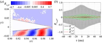
where  $N$ is the number of PIV snapshots rather than that of the sound pressure measurements, as the latter sampling frequency is 10 times higher. The correlation map in figure 22(a) illustrates an alternative pattern of negative and positive contour levels, which is similar to the results for aerofoils (Nakano et al. Reference Nakano, Fujisawa and Lee2006; Pröbsting et al. Reference Pröbsting, Serpieri and Scarano2014) and cylinders (Henning et al. Reference Henning, Kaepernick, Ehrenfried, Koop and Dillmann2008) with tonal noise generation. The region with strong periodic patterns of the correlation coefficient was reported to be dependent on the separation region (Nakano et al. Reference Nakano, Fujisawa and Lee2006). Comparing the correlation map of
 $R _{v,p^{\prime }}$ in figure 22(a) with the first and second POD mode patterns as shown in figure 18(a,b), a high similarity in terms of periodic patterns is noticed. The POD modes represent the velocity fluctuations in the flow field, which are the source of hydrodynamic pressure fluctuations scattering noise into the far field at the TE. The region with strong velocity fluctuations has a strong correlation with the far field noise, and thus the first and second POD modes with higher turbulent energies show a similar pattern to the correlation map.
(a) Contour of the correlation coefficient between the transverse velocity component and the acoustic pressure signal. The time delay has been corrected for the propagation time between TE and the location of the microphone; (b) correlation between the time coefficients of POD modes and sound pressure. Here,  $u_\infty = 12\,{\rm m}\,{\rm s}^{-1}$.

The correlation coefficient between the first POD mode and the sound pressure  $R{_{c_{1}\!,p^{\prime }}}$ is shown in figure 22(b). The maximum magnitude of the correlation coefficient
 $R_{c_1\!,p^{\prime }}$ reaches 0.84 for the first mode, which exceeds the maximum value found for the correlation between the transverse velocity component and the sound pressure (0.7) in figure 22(a). This indicates that POD analysis has suppressed background noise or turbulence (Henning et al. Reference Henning, Kaepernick, Ehrenfried, Koop and Dillmann2008) and filtered out flow field fluctuations that are incoherent with the large-scale motion (van Oudheusden et al. Reference van Oudheusden, Scarano, van Hinsberg and Watt2005; Lengani et al. Reference Lengani, Simoni, Ubaldi and Zunino2014). In the case of the third and fifth modes, the correlation coefficients reach maxima of approximately 0.21 and 0.06, respectively, which means their contributions to the noise emission are weak in comparison.
6.2. Condition with comparable primary and secondary side tones
The sound spectra at  $u_\infty = 18\,{\rm m}\,{\rm s}^{-1}$ featured comparable magnitudes of primary and secondary side tones and peaks at similar frequencies (see figure 3c) were observed in the velocity spectra (see figure 13). The respective flow structures for these two side tone sets are analysed.
6.2.1. POD modes
At  $u_\infty = 18\,{\rm m}\,{\rm s}^{-1}$ the TKE for the first, second and third modes is similar at respectively 10.9 %, and 10.4 % and 9.4 %, as shown in figure 23(a). Higher modes contain lower TKE, which means their contributions to the fluctuation are less significant in comparison with the first to third modes. Figure 23(b) shows the spectra of
 $c_n$ for the six POD modes. The spectral shapes of modes 1
 $-$6 are similar, featuring a broadband hump in the low-frequency range around 12 Hz and another broadband hump in the mid-frequency range around 554 Hz. The mode with the largest energy content at 554 Hz is mode 1, and the mode with the largest energy content at 11.5 Hz is mode 3.
(a) Energy distribution of the POD modes; (b) frequency spectra of mode time coefficients  $c_n$. Here,
 $u_\infty = 18\,{\rm m}\,{\rm s}^{-1}$.

The first $-$sixth POD modes are selected to depict the dominant modal features. Figure 24 shows velocity vectors superimposed on velocity contour of
 $v^{\prime }$. All six modes show similar patterns with alternating signs of velocity fluctuations on the pressure side. For the sixth mode the wavelength of these structures on the pressure side is reduced. The actual flow structures contributing to these modes will be discussed together with the mode time coefficients.
The flow structures corresponding to the first to sixth mode (a–f). Here,  $u_\infty = 18\,{\rm m}\,{\rm s}^{-1}$.

6.2.2. Sound pressure fluctuation: contributions from the POD modes
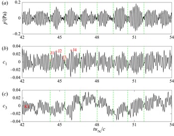
Figure 25(a) shows the time history of acoustic pressure. The filtered sound pressure is characterised by high-frequency oscillations superimposed by low-frequency amplitude modulation. The high-frequency oscillation corresponds to the dominant tone, i.e. 554 Hz, while the frequency of the amplitude modulation (see figure 25b) corresponds to the frequency interval of primary side tone set, i.e. 50 Hz.
Time histories of sound pressure and POD mode time coefficients in the time slot of  $t u_\infty /c =$ 42–54,
 $u_\infty = 18\,{\rm m}\,{\rm s}^{-1}$. (a) Sound pressure; (b)
 $c_1$; (c)
 $c_3$. The green lines represent the instants with low values of
 $p^{\prime }$ amplitude envelope. J1 and J3 represent instants with low values of
 $c_1$ amplitude envelope, and the opposite for J2 and J4.

The corresponding time histories of the dominant POD mode coefficients  $c_n$ are presented in figure 25(b,c). The high-frequency oscillation of the dominant one is present in both coefficients
 $c_1$ and
 $c_3$. The frequency of the amplitude modulation of
 $c_1$ is approximately 50 Hz, which is equal to the frequency interval of the primary side tone set. Over the time range shown here (
 $t u_\infty /c =42\unicode{x2013}54$), the low-frequency fluctuation is hardly noticeable for the time coefficient
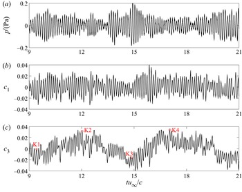
 $c_3$. Therefore, the evidence of low-frequency fluctuation is searched over different time domains. Figure 26 shows the comparison of sound pressure time history and modal coefficients for
 $t u_\infty /c =9\unicode{x2013}21$. Here, the low-frequency fluctuation of
 $c_3$ is apparent at approximately 11.5 Hz, which corresponds to the frequency interval of the secondary side tone set. In contrast, the time coefficient of
 $c_1$ over this time range does not feature an obvious low-frequency, periodic oscillation. Therefore, it is concluded that the amplitude modulation due to
 $c_1$ and
 $c_3$ may be intermittent.
Time histories of sound pressure and POD mode time coefficients in the time slot of  $t u_\infty /c =$ 9–21. (a) Sound pressure; (b)
 $c_1$; (c)
 $c_3$; K1–K4 represent instants with large values of
 $c_3$ amplitude envelope. Here,
 $u_\infty = 18\,{\rm m}\,{\rm s}^{-1}$.

The high-frequency oscillations representing the vortex shedding are similar to those elaborated on in § 6.1. The marked symbols of J1–J4 in figure 25 indicate the instants with peak values of the amplitude envelope  $c_1$ which accounts for the frequency interval of the primary side tone set. The flow fields at these instants are displayed in figure 27. At instant J1, the instantaneous flow field corresponding to a low value of
 $c_1$ amplitude envelope is shown in figure 27(a). On the pressure side the shear layer is separated and vortex break-up can be identified near
 $x/c = 0.98$. An incoherent vortex near the TE is consistent with the low amplitude of sound pressure
 $p^{\prime }$ since the pressure fluctuation induced by concentrated vortex shedding is weak. Half a period of the modulation later, at instant J2, the value of
 $c_1$ attains a local maximum of the amplitude envelope, and the corresponding instantaneous flow field is shown in figure 27(b). With respect to J1, the shear layer rolls up into discrete vortices from
 $x/c = 0.96$, with a space interval of 0.04
 $c$ clearly visible near the TE. Strong vortex shedding is consistent with the high amplitude of sound pressure
 $p^{\prime }$. Another semi-period of the modulation frequency later, at instant J3, the value of
 $c_1$ attains another local minimum of the amplitude envelope. The corresponding flow field in figure 27(c) looks similar to figure 27(a) at instant J1 in terms of shear-layer break up into small vortical structures from
 $x/c = 0.96$. At instant J4, a shed vortex is rolled up near
 $x/c = 0.95$, and has an interval of 0.045
 $c$ with subsequent vortex. Therefore, the first mode, or amplitude modulation of sound pressure
 $p^{\prime }$ at 50 Hz, is ascribed to the intermittent vortex shedding and break-up of shear layer on the pressure side, which results in an amplitude modulation to the sound pressure.
Flow fields of spanwise vorticity contours superimposed by velocity vectors for J1–J4 in (a–d) (see figure 25b) and for K1–K4 in (e–h) (see figure 26c). The break-up and coherent vortices are annotated, and the arrows indicate the position of vortex roll-up. Here,  $u_\infty = 18\,{\rm m}\,{\rm s}^{-1}$.

The flow fields at the instants with peaks of  $c_3$ amplitude envelope, K1–K4, are presented in figure 27(e–h), which help to explain the secondary modulation of the sound pressure. At instant K1, the instantaneous flow field corresponding to a peak value of the amplitude envelope is shown in figure 27(e). Although the flow looks similar to figure 27(a), a significant difference at K1 is that it features a coherent vortex structure at
 $x/c = 0.98$, while vortex break-up is observed at J1 near
 $x/c$ = 0.98. Half a period of the low-frequency modulation later, at instant K2, the value of
 $c_3$ attains a local maximum of the amplitude envelope, and the corresponding instantaneous flow field is shown in figure 27( f). With respect to K1, the occurrence of vortex roll-up occurs earlier, and the vortex appears to be less coherent near the TE when compared with K1. This earlier roll-up in turn is related to the oscillation of the separation bubble as explained in the discussion of figure 21. Similarly, the vortex near the TE at instant K3 is coherent, but less coherent at K4. Therefore, the third mode, or low-frequency modulation around 11.5 Hz, is ascribed to the oscillation of the separation bubble as discussed in § 6.1.2.
6.3. Condition with dominant secondary side tone set
Sections 6.1 and 6.2 showed flow cases with secondary side tones appear at  $u_\infty = 12$ and
 $18\,{\rm m}\,{\rm s}^{-1}$. Yet, in these cases, the corresponding modes only contain low TKE. In contrast, at
 $u_\infty = 21\,{\rm m}\,{\rm s}^{-1}$, the noise and velocity spectra are both dominated by the secondary side tones.
6.3.1. POD modes
Similar to the modal analyses for  $u_\infty = 12$ and
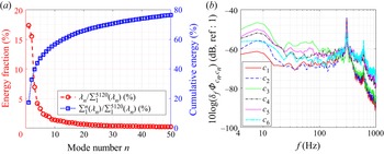
 $18\,{\rm m}\,{\rm s}^{-1}$, a large amount of energy is captured by a small number of modes. The first and second modes represent 28.4 % and 8.2 % of the total TKE, respectively, as shown in figure 28(a). The frequency spectra of the first two modes are highly similar, as shown in figure 28(b), and the magnitudes at 12.5 Hz are equal. The third to sixth modes occupy
 $5.0\,\% , 4.6\,\%, 3.2\,\%, 2.3\,\%$ of total TKE, respectively, and the spectra of these modes show strong humps in the high-frequency range (around 600 Hz), whereas the low-frequency humps (around 12.5 and 25 Hz) become relatively lower when compared with those of the first and second modes.
(a) Energy distribution of the POD modes; (b) frequency spectra of mode time coefficients  $c_n$. Here,
 $u_\infty = 21\,{\rm m}\,{\rm s}^{-1}$.

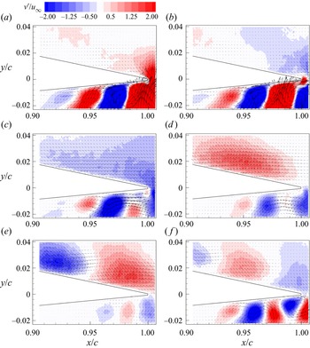
The first six POD modes are shown in figure 29. Modes 1 and 2 as shown in figure 29(a) identify a region (large negative values of the mode) which oscillates and is completely different from the first and second modes observed for  $u_\infty =12$ and 18
 ${\rm m}\,{\rm s}^{-1}$. This motion characterises the ‘wavering’ of the separated shear layer (Lengani et al. Reference Lengani, Simoni, Ubaldi and Zunino2014). Modes 3 and 4 show alternative vertical velocity fluctuations which were observed for other cases as well and represent the vortex convection. The wavelength of the velocity pattern has an increasing trend in downstream direction. Modes 5 and 6 also show coherent flow patterns, yet their structure is embedded within smaller-scale structures, which means the flow structure is a combination of several flow features at substantially different scales.
The flow structures corresponding to the first to sixth mode (a–f). Here,  $u_\infty = 21\,{\rm m}\,{\rm s}^{-1}$.

6.3.2. Sound pressure fluctuation: contributions from the POD modes
The time history of far-field sound pressure is presented in figure 30(a). It is characterised by high-frequency oscillation and low-frequency amplitude modulation. The low-amplitude instants are represented by vertical dashed lines (green). A similar alternating history of quiet and intense sound pressure was also observed by Sanjose et al. (Reference Sanjose, Towne, Jaiswal, Moreau, Lele and Mann2019). The frequency of the high-frequency oscillation equals that of the main tone of the acoustic spectra, i.e. 600 Hz (compare figure 3d). The frequency of the amplitude modulation is around 12.5 Hz, which equals the frequency interval of the secondary side tones as shown in figure 3(d).
Time histories of sound pressure and POD mode time coefficients. (a) Sound pressure; (b) POD mode coefficient  $c_1$; (c)
 $c_3$. The vertical dashed lines (green) represent the instants with low values of
 $p^{\prime }$ amplitude envelope. J1–J4 represent instants with large values of
 $c_1$ amplitude envelope. Here,
 $u_\infty = 21\,{\rm m}\,{\rm s}^{-1}$.

Figure 30(b,c) shows the time coefficient of the POD modes. By comparing the time history of  $p^{\prime }$ with those of
 $c_1$ and
 $c_3$, it is found that the amplitude modulation of the noise signal is consistent with that of
 $c_3$. Furthermore, the amplitude modulation of
 $c_3$ is clearly consistent with the phase of the
 $c_1$ fluctuation, which implies they are driven by the same flow phenomenon.
The marked symbols of J1–J4 indicate high-amplitude instants of  $c_1$. The flow fields at these instants are displayed in figure 31 to discuss the low-frequency fluctuation of
 $c_1$ and amplitude modulation of
 $c_3$. At instant J1, the instantaneous flow field, corresponding to both a local minimum of
 $c_1$ as well as a low value of the
 $c_3$ amplitude envelope, is shown in figure 31(a). It can be seen that the shear layer on the pressure side is reattached to the aerofoil wall. Half a period of the low-frequency oscillation later, at instant J2, the value of
 $c_1$ attains a local maximum and the amplitude envelope of
 $c_3$ has a high value. The corresponding instantaneous flow field is shown in figure 31(b). With respect to J1, the shear layer on the pressure side is separated from the aerofoil surface and the K–H instability induced vortex roll-up from the shear layer is visible near the TE. Another semi-period of the main tone frequency later, at instant J3, the value of
 $c_1$ attains another local minimum and the amplitude envelope of
 $c_3$ attains lower values. The corresponding flow field in figure 31(c) looks similar to that in figure 31(a) at instant J1 in terms of shear layer attachment. At instant J4, the shed vortex appears and looks similar to that at instant J2. Therefore, the first and third modes are ascribed to the shear-layer reattachment and separation near the TE, which is a result of the bubble movement as discussed with figure 21.
Flow fields in (a–d) correspond to instants of J1–J4 (see figure 30). Here,  $u_\infty = 21\,{\rm m}\,{\rm s}^{-1}$.

7. Conclusion
For the NACA 0012 aerofoil in the Reynolds number range of  $2 \times 10^{5}$–
 $7 \times 10^{5}$ a single tone dominates tonal emission at low Reynolds numbers. With increasing Reynolds number, multiple side tones appear before the spectral characteristic changes to broadband. Two distinct sets of side tones have been identified in the sound spectra. The frequency interval of tones in the primary set agrees well with the feedback model suggested by Arbey & Bataille (Reference Arbey and Bataille1983), which is most noticeable at moderate velocities. The secondary set is present in all velocity regimes with a frequency interval equal to approximately 1/4–1/3 of the primary one. While the primary side tone set has been discussed extensively in the literature, the secondary side tones have not been identified or discussed. However, as acoustic measurements show, they can be important for some flow conditions.
Time-averaged flow fields show an LSB on the pressure side. Triple peaks of the wall-tangential velocity fluctuations are observed, which were previously described as necessary conditions for tonal noise generation. The wall-normal velocity fluctuations show one peak near the surface. A flow condition with one dominant acoustic tone shows the highest magnitude of wall-normal velocity fluctuations, whereas the case with multiple tones of comparable sound power shows the lowest magnitude. The instantaneous flow fields show the development of the shear layer, vortex roll-up and vortex break-down from the upstream to the downstream region near the aerofoil's TE. The roll-up location is located further downstream at lower velocity and the vortex is therefore more coherent near the TE. The wall-normal velocity spectra agree well with the acoustic ones in terms of spectral shape as expected. The energy content increases downstream for all broadband components, yet the tone magnitude reaches a maximum around  $x_t/c = -0.03$.
POD analysis revealed the most energetic flow structures in the vortex shedding process. Time history comparison and correlation with the far-field sound pressure linked POD modes to the acoustic emission. For the flow condition with one dominant tone, the most energetic modes comprise pairs of the flow modes which are dominated by the vortex convection process. For the flow condition with comparable magnitude of primary and secondary side tone sets, the primary tone set is dominated by amplitude modulation of the convecting vortices related to the first mode, and the secondary tone set is dominated by the low-frequency oscillation represented by the second and third modes. For flow conditions characterised by the prevalence of the secondary side tone set, the first mode has approximately 30 % of total TKE and resembles a low-frequency oscillation due to shear-layer separation and attachment near the TE. The low-frequency oscillation was observed for all three cases. The corresponding mode is the third most energetic mode for  $u_\infty$ = 12 and
 $18\,{\rm m}\,{\rm s}^{-1}$, while it is the first mode for
 $u_\infty = 21\,{\rm m}\,{\rm s}^{-1}$. In other words, with increasing Reynolds number, the secondary modulation type progressively prevails over the primary type.
By aligning the time histories between sound pressure and time coefficients of the POD modes, flow mechanisms for the primary and secondary side tone sets are explained. The primary set of tones is related to intrinsic modulation due to frequency selection criterion of the feedback loop. The secondary modulation is related to a coupling of the hydrodynamics in the nonlinear part of the amplification process due to an intrinsic oscillation of the separation bubble. Separation bubble oscillation in experiments is receptive to the shear-layer fluctuation of the wind-tunnel open jet. It should be mentioned that low-frequency oscillation of an LSB is also widely reported in numerical simulations due to other sources of disturbances (Alam & Sandham Reference Alam and Sandham2000; Maucher et al. Reference Maucher, Rist, Kloker and Wagner2000; Spalart & Strelets Reference Spalart and Strelets2000; Wissink & Rodi Reference Wissink and Rodi2002, Reference Wissink and Rodi2003, Reference Wissink and Rodi2004) or it can be self-sustained (Jones et al. Reference Jones, Sandberg and Sandham2008).
It should be noted that the secondary side tones discussed in the present study have been observed for the particular combination of flow conditions and geometry described here. By changing the free-stream velocity for a specific aerofoil model the transition process is also modified due to the variation of Reynolds number and turbulence intensity. Transition characteristics influence the flow dynamics and thus the tonal noise generation. Moreover, the Mach number changes, which is an important factor for aeroacoustic problems. Therefore, the results cannot be quantitatively generalised to arbitrary flow conditions. However, it is important to be aware of the possible occurrence of the secondary modulation described here.
Acknowledgements
The authors acknowledge the support of graduate students C. Li and H. Zhang at Southern University of Science and Technology for conducting wind-tunnel tests.
Funding
Y.Y. and Y.L. thank the AVIC General Aircraft Research Institute (Grant No. AG-EX_HT_024), the National Natural Science Foundation of China (Grant Nos 11802114 and 92052105) for the support. S.P. and Y.L. thank the National Natural Science Foundation of China (Grant No. 11872248) for the support.
Declaration of interests
The authors report no conflict of interest.
Appendix A
For the NACA 0012 aerofoil with the same chord length of 0.3 m but at a different angle of attack, i.e.  $\alpha = 1^{\circ }$, the noise emissions were measured in the velocity range of 11.2–23.3
 ${\rm m}\,{\rm s}^{-1}$. The acoustic spectra for the selected velocities
 $u_\infty = 11.2, 18$ and
 $21\,{\rm m}\,{\rm s}^{-1}$ are shown in figure 32(a–c), respectively. Three characteristic shapes are identified, which are consistent with those discussed for
 $\alpha = 2^{\circ }$. At
 $u_\infty = 11.2\,{\rm m}\,{\rm s}^{-1}$, The spectrum is defined by tones with the dominant tone at
 $f_{10}^{(1)}$ exceeding the first side tone of the primary set at
 $f_{11}^{(1)}$ by 16 dB as shown in figure 32(a). At
 $u_\infty = 18\,{\rm m}\,{\rm s}^{-1}$, the spectra become progressively broadband and the difference between the dominant tone (at
 $f_{12}^{(1)}$) and the first side tone of the primary set decreases to 6 dB as shown in figure 32(b). At
 $u_\infty = 21\,{\rm m}\,{\rm s}^{-1}$, the spectral hump becomes progressively broader at the top as shown in figure 32(c). Throughout this progression, the secondary side tone set becomes dominant.
Acoustic spectra at three velocities: (a)  $11.2\,{\rm m}\,{\rm s}^{-1}$; (b)
 $18\,{\rm m}\,{\rm s}^{-1}$; (c)
 $21\,{\rm m}\,{\rm s}^{-1}$. Here,
 $\alpha = 1^{\circ }$.

The contour map of the acoustic spectra is shown in figure 33(a). Ladder-type structures are identified by the ridges (red). Tonal frequencies are extracted from the contour map and shown in figure 33(b). The definition of the different symbols follows that in figure 32(a), where the dominant tone follows the power law of  $k(n+0.5)u_\infty ^{0.85}$. The primary side tone set (triangle, blue) and secondary side tone set (circle, red) are located around the dominant tone. The factor
 $k$ for curve fitting in figure 33(b) is approximately 3.1.
Dependence of tonal noise on free-stream velocity. (a) Spectra contours of noise emission; (b) dominant, primary and secondary side tones. Here,  $\alpha = 1^{\circ }$.

The frequency intervals of the primary and secondary side tone sets are shown in figures 34(a) and 34(b), respectively. The frequency interval of the primary side tones vs flow velocity approximately follows the power law of  $\Delta f_n \sim 3.1u_\infty ^{0.85}$. In the context of (3.2) the feedback-loop length is 0.96
 $c$, which is longer than that at
 $\alpha = 2^{\circ }$ (see § 3). The frequency interval of the secondary side tones vs flow velocity follows the fit
 $\Delta f_n^{(2)} \sim 0.6u_\infty$, which is consistent with the inflow disturbance as evaluated in figure 16(b).
(a) Frequency interval of the primary side tones; (b) frequency interval of the secondary side tones. Here,  $\alpha = 1^{\circ }$.

Appendix B
The boundary layer profiles as well as the displacement thickness, momentum thickness and shape factor on the pressure side are plotted in figure 35. The FoV extends over the thickness of the boundary layer for  $u_\infty = 18\,{\rm m}\,{\rm s}^{-1}$ and
 $21\,{\rm m}\,{\rm s}^{-1}$, whereas the outer part of the boundary layer is not captured for
 $u_\infty = 12\,{\rm m}\,{\rm s}^{-1}$, and thus boundary parameters are only characterised for
 $u_\infty = 18\,{\rm m}\,{\rm s}^{-1}$ and
 $21\,{\rm m}\,{\rm s}^{-1}$. The normalised displacement and momentum thicknesses are
 $O(10^{-3})$, which are in good agreement with data reported in the literature (Pröbsting & Yarusevych Reference Pröbsting and Yarusevych2021). Further downstream, the decreasing shape factor implies that the flow gradually becomes more turbulent, which is consistent with the vortex break-up near the TE as shown in figure 11. Moreover, the value of the shape factor decreases when the velocity increases, as the LSB moves upstream and the flow is therefore more turbulent near the TE.
Boundary layer characteristics on the pressure side. (a) Wall-tangential velocity profile; (b) displacement thickness; (c) momentum thickness; (d) shape factor. Here,  $\alpha = 2^{\circ }$.

Additionally, the boundary layer characteristics on the suction side are plotted in figure 36. The shape factor of approximately 1.6 in figure 36, which falls in the range  $H = 1.3\unicode{x2013}1.4$ typical for turbulent flows (Schlichting & Gersten Reference Schlichting and Gersten2017). A similar shape factor of 1.7 at the TE for a tripped NACA 0018 aerofoil at
 $\alpha = 0^{\circ }$ and
 $Re = 2.63\times 10^{5}$ was reported (León, Merino-Martínez & Ragni Reference León, Merino-Martínez and Ragni2016). The flow being turbulent near the TE on the suction side for all three velocities is an indication for the tonal noise being generated by pressure side events.
Boundary layer characteristics on the suction side. (a) Wall-tangential velocity profile; (b) displacement thickness; (c) momentum thickness; (d) shape factor. Here,  $\alpha = 2^{\circ }$.