HOW HOLC REPAIRED CREDIT CHANNELS

Recent events have shown that it is difficult to reverse, or even moderate, disruptions in housing and mortgage markets once they have occurred. The same lesson was learned during the 1930s. Low interest rates on home loans, for example, normally stimulate home sales, home prices, and residential construction, but cheap money by itself has not promoted a recovery in residential real estate during the current mortgage crisis. One challenge in assessing the impact of HOLC, therefore, is to understand how a massive substitution of public for private mortgage credit between 1933 and 1936 improved outcomes in housing markets.

Ben Bernanke, Mark Gertler, and Simon Gilchrist provide a framework within which to conceptualize the issue.Footnote ¹¹ They emphasize that disruptions in credit markets for small business and households are capable of transmitting and amplifying negative economic shocks into large aggregate fluctuations, a phenomenon they refer to as the financial accelerator. Lenders in these personalized markets use costly contractual and institutional mechanisms (such as down payments, collateral, or scheduled refinancing) to mitigate borrowers' informational advantages regarding project quality, effort, and outcomes. The accelerator arises because the costs associated with these mechanisms spike after a negative shock, so that credit becomes more expensive and more difficult to secure just when small businesses and households need to rely on it most.

One specific channel through which the accelerator operates is the use of borrowers' balance sheets to assess creditworthiness and to set loan rates.Footnote ¹² When forces external to the credit market decrease the value of assets held by businesses and households, for example, it becomes harder for them to post collateral that lenders insist upon before approving a loan. As a result, the supply of credit contracts, interest rates rise and the shock is transmitted even further. Similar impacts are felt after the failure of intermediaries that serve information-intensive borrowers. This second component of the financial accelerator arises because lenders in these markets develop relationships with their customers and accumulate information about them that lowers the costs of making and enforcing contracts. When agencies like these fail, information about borrowers is lost, the cost of credit intermediation increases, and the supply of credit contracts. The financial accelerator deepens crises within loan markets, therefore, because the contractual and institutional mechanisms that are used to control asymmetries of information in these markets transmit distress among some borrowers and lenders to other market participants.

The literature provides compelling circumstantial evidence that both elements of the financial accelerator were at work in the mortgage market during the early 1930s. Frederic Mishkin, for example, shows that the large decrease in household consumption at the onset of the Depression resulted from deteriorations in household balance sheets as stock values and home prices plummeted, and the level of real household debt increased with deflation.Footnote ¹³ These same developments would have negatively affected the creditworthiness of households and their ability to meet the down payment or debt-service requirements for a mortgage. Bernanke, on the other hand, shows that a measure of bank failures, his proxy for the “cost of credit intermediation,” explains some of the decline in real economic activity during the early 1930s.Footnote ¹⁴ Although his empirical analysis focused on the banking system, Bernanke emphasizes that other evidence indicates that similar disruptions occurred among home mortgage lending specialists during the 1930s.Footnote ¹⁵

A final piece of evidence that a financial accelerator was at work during the mortgage crisis of the early 1930s is Hoagland's eyewitness testimony that “our whole value structure can be thrown out of balance by relatively slight shocks,” and “[w]hen such a delicate structure is once disorganized, it is a tremendous task to get it into a position where it can again function normally.” He describes an environment in which homeowners were unable to qualify for credit, existing mortgage lenders were severely distressed, and the housing market was in a downward spiral of home foreclosures and decreases in home values. All this bad news led to additional deterioration in household balance sheets and further disruptions in intermediated real estate lending channels.

Against this backdrop, HOLC needs to be evaluated as a mechanism that attempted to mitigate both channels of the financial accelerator by purchasing distressed mortgages from lenders and offering loan modifications to borrowers. The program was not designed, in particular, to make new home mortgages or to directly stimulate home construction; its mission was limited to serving homeowners who could not secure refinancing from a private lender. There were at least three groups of homeowners in 1933 that only HOLC could have helped. The first had purchased homes during the 1920s using the 3- to 5-year balloon loans that were typical at the time. Many of these loans reached maturity between 1930 and 1933 at which time many of these homeowner discovered that they were no longer eligible for a loan renewal because the collateral they could offer—their homes—had decreased significantly in value. A second group included households that had become delinquent on property tax payments as well as their mortgages; HOLC had authority, unlike private lenders, to wrap tax arrearages into refinanced loan balances so that foreclosure could be avoided.

A third group that HOLC was uniquely positioned to help in 1933 were homeowners who had become trapped in one of the thousands of failed Building & Loan associations that became “frozen” as they gradually liquidated. The standard B&L loan at this time combined a non-amortizing mortgage with a contract to purchase shares in the association by means of weekly or monthly dues. Under this arrangement, the borrower's share account served as a sinking fund that eventually grew equal in value, and therefore canceled, the principal of the loan. Borrowers in frozen B&Ls during the early 1930s, however, watched the value of their sinking funds fall as their institution took losses as the pace of defaults and foreclosures picked up in the early 1930s. In this circumstance, a borrower had strong incentives to withhold share installment and loan payments so as not to throw good money after bad. By securing HOLC refinancing, these borrowers were able to extract themselves from the failing B&Ls and protect themselves from further risks and losses.Footnote ¹⁶

Beyond serving borrowers who could not refinance in the private market, HOLC offered loan modification packages that no private intermediary could have matched. The agency's standard contract was a 15-year, fully amortized mortgage with a 5 percent rate of interest at a time when borrowers in the private market paid 6 percent and higher on short-term, balloon loans.Footnote ¹⁷ HOLC was also authorized to lend up to 80 percent of a generously appraised home value and to waive amortized principal payments for the first three years if the borrower required that consideration.Footnote ¹⁸ The agency's lending terms were so generous that it had to screen out and discourage applications from ineligible homeowners. The purpose of offering these terms, however, was to offer a mortgage product for hundreds of thousands of distressed borrowers who could not qualify for refinancing under the terms offered by private lenders.Footnote ¹⁹

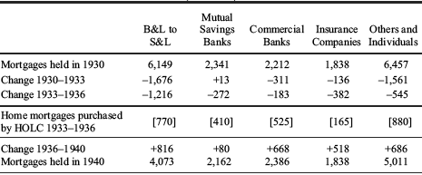
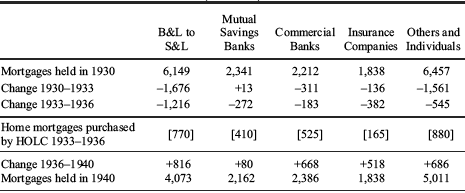
The other side of HOLC's business model, the purchase of distressed mortgages, reduced and repaired distress among investors. The agency paid for mortgages with its own guaranteed bonds, so private lenders that sold to HOLC shored up their own balance sheets by substituting safe, marketable assets for distressed residential loans.Footnote ²⁰Table 1 illustrates the importance of the purchases by placing them against the backdrop of changes in the volume of debt held by all major categories of home mortgagors during the 1930s. As the crisis took hold between 1930 and 1933, the nation's total home mortgage debt decreased by 17 percent ($3.6 billion) with the largest reductions in the portfolios of B&Ls and individual investors.Footnote ²¹ The total decreased by another 17 percent between 1933 and 1936, but this time the decline was almost completely offset by increases in HOLC's mortgage holdings. During the period, moreover, HOLC touched all major lending groups with purchases that equaled two-thirds of the reduction in B&L mortgage holdings and more than the total decrease in the portfolios of individual investors, mutual savings banks, and commercial banks (see the third and fourth rows of Table 1). HOLC purchases were also large when compared to the $2.8 billion expansion in private lending that occurred between 1936 and 1940. Once again, its loan purchases equaled 80 percent or more of the increase in mortgage holdings for all lending groups except insurance companies.

TABLE 1

MORTGAGES HELD BY MAJOR LENDING GROUPS ON 1–4 FAMILY NONFARM HOMES AND PURCHASED BY HOLC, 1930–1940 ($ millions)

Source

Grebler, Blank, and Winnick, Capital Formation, N-4; and U.S. Housing and Home Finance Agency, Final Report (1952), iv.

HOLC was designed, therefore, to provide badly needed refinancing to distressed homeowners while simultaneously strengthening private lenders. We are interested here in assessing whether these activities repaired disruptions in mortgage lending channels and reduced distress in local housing and mortgage markets. There are other possibilities, of course. HOLC activity could have been allocated to provide local economies with general relief or to garner political favor. In these cases, factors such as unemployment or political variables, rather than local housing distress, would have determined the spatial distribution of HOLC activity, while the lending itself would have had only weak impacts on residential market outcomes. We find no evidence that supports either alternative hypothesis.

ALLOCATION OF HOLC LOANS ACROSS COUNTIES

By name and legislative intent, HOLC was a program designed to assist distressed homeowners, but we still do not know why nearly two million households applied to HOLC for mortgage relief or how the relief was allocated across the nation's local mortgage markets.Footnote ²² The Roosevelt administration believed that the need for HOLC was urgent and used a national radio address to explain the purpose, procedures and eligibility requirements of the program the day after the Home Owners' Loan Act was signed into law on June 11, 1933. The public campaign encouraging distressed homeowners to apply worked so well that the first HOLC office in New York had already received 5,000 applications by mail when it opened its doors on August 14 and found hundreds more homeowners waiting to apply. Given the overwhelming public response, the HOLC focused that summer and fall on hiring staff to open state and local HOLC offices, to receive applications from borrowers, and to encourage lenders to delay foreclosure proceedings until the agency had processed each case. As a result, HOLC had refinanced only 50,000 of the 700,000 homeowners that had applied for relief by December 1933 and the agency continued to operate for the next year with a six-month backlog of cases.Footnote ²³

After the first few months, the interplay between HOLC and homeowners became more complex. The agency began in fall 1933 to include information about rejected loan applications in its regular press releases and to explicitly discourage applications from homeowners who did not meet the program's eligibility requirements or who could not demonstrate sufficient distress.Footnote ²⁴ By then, it had also become obvious that private lenders, as well as distressed homeowners, would play an important role in determining the volume of applications and the rate of program participation. Some applications, for example, came from borrowers who were encouraged by their lenders to apply, while one-tenth of all HOLC loans were made through wholesale operations in which the Reconstruction Finance Corporation and HOLC worked together to refinance mortgage loans on the books of failed intermediaries.Footnote ²⁵ The agency, moreover, regularly reported the number of applications that had been withdrawn after HOLC staff had assisted the private parties to reach agreement on their own refinancing package.Footnote ²⁶ Finally, 7 percent of HOLC applications failed because lenders refused to sell their loans even though the agency systematically set home appraisals high so that lenders would not be forced to take a haircut.Footnote ²⁷ The record clearly indicates, therefore, that application and participation rates in the HOLC program depended on complex interactions among homeowners, private lenders, and HOLC staff.

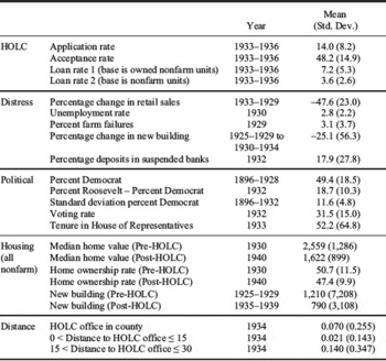
The county-level data we employ here are too coarse to identify or assess the determinants of the interplay among all the parties. We focus instead on how the outcomes of these negotiations—HOLC application and participation rates—were influenced by the characteristics of local housing markets in which these interactions took place. We address these issues by examining the determinants of the number of HOLC applications that were made in each county in the United States between 1933 and 1936 and the number of these that were accepted into the program. The Federal Home Loan Bank Board reported these data in its fifth annual report. We scale them here by the number of occupied and owner-occupied nonfarm housing units in each county as measured in the Census of 1930 in order to construct four measures of HOLC loan activity: first, the number of HOLC applications in each county as a percentage of owner-occupied nonfarm homes in 1930 (application rate); second, the percentage of HOLC applications accepted for purchase and refinancing (acceptance rate); third, the number of homes refinanced by HOLC as a percentage of the number of owner-occupied homes in 1930 (loan rate 1); and fourth, the number refinanced as a percentage of all nonfarm homes in 1930 (loan rate 2).Footnote ²⁸ The first panel of Table 2 shows that 14 percent of owner-occupied households in the average county applied for HOLC loans, that an average of just under 50 percent of applications were accepted, and that HOLC financed an average of just over 7 percent of owned homes, or 3.6 percent of all nonfarm homes.

The goal of the analysis is to assess whether HOLC lending was directed at disruptions in local housing markets or for other purposes that have been mentioned in the literature. HOLC loans could have been used, to begin with, to provide general relief to homeowners who had become unemployed or had lost income in other ways during the Depression—there is evidence, in fact, that HOLC was the only loan program sponsored by the New Deal that was distributed in response to general measures of relief and recovery.Footnote ²⁹ A second possibility is that HOLC refinancing was used for political purposes rather than to relieve credit market disruptions. HOLC loans provided borrowers with low-cost mortgages that carried much more liberal terms than private loans, so cheap credit could have been distributed to gain political advantage.Footnote ³⁰

TABLE 2

SUMMARY STATISTICS FOR KEY VARIABLES

Note:

Summary statistics for the demographic, economic structure and income variables are available in Appendix Table 1 of the online appendix.

We employ a modified version of the empirical model that Fishback, Kantor, and Wallis used to examine variations in county-level per capita spending levels for 20 New Deal grant and loan programs, including HOLC.Footnote ³¹ They included demographic controls (population, density and percent urban, illiterate, black, and race other than white or black), measures of economic structure and income (average farm size, percent of county in farmland, retail sales per capita, and percent of households filing tax returns), proxies for distress (unemployment rate in 1930, percent farm failures, and percent change in retail sales between 1929 and 1933), and a rich set of political variables.

We augment Fishback, Kantor, and Wallis's model in several ways to incorporate factors that could have influenced the allocation of HOLC refinancing across local markets. For example, we extend their demographic specification by including measures of the age composition in each county and the percent married, female, and foreign born. We also incorporate additional information about economic structure by accounting for the share of gainful workers employed in manufacturing, retail, and wholesale establishments.Footnote ³² We capture local financial market distress in the specification, moreover, by including the percent of bank deposits in each county that were held at the end of 1932 in banks that ended up suspending payments in 1933. Finally, and most importantly, we measure housing market distress in each county with the percentage change between 1925–1929 and 1930–1934 in the number of nonfarm dwelling units built.Footnote ³³ We consider this a key measure of disruption in local housing markets that should have influenced the perceived need for HOLC refinancing among borrowers and the judgments of HOLC administrators about that need.

We also include additional independent variables to capture factors that should have influenced eligibility for HOLC refinancing and, therefore, both application and acceptance rates. A homeowner had to be encumbered to be eligible for an HOLC loan, so we add the natural logarithms of nonfarm median home values in 1930 and the number of new homes built between 1925 and 1929 since newer and higher-priced homes were more likely to have been mortgaged. High-priced homes of recent vintage should also have appraised for greater property values in 1933, so these same two variables could have been associated with higher acceptance as well as application rates. We also include the nonfarm homeownership rate in each county to see if loan applications or acceptances were sensitive to the mix of owned and rented housing in each local market.Footnote ³⁴

Finally, we add distance from the nearest HOLC office location to reflect one of the agency's most impressive accomplishments—in a matter of months it created a national loan origination and servicing network. By 1934 HOLC had opened more than 200 offices, with at least one in every state.Footnote ³⁵ Office location mattered to the agency's reach because distance increased the costs of mortgage lending for its staff and for borrowers—appraisals required onsite inspections and applications and documents had to move among homeowners, county officials, and HOLC staff. We include an indicator for counties containing an HOLC office, another for counties located within 15 miles of an office but not containing an office, and a third for counties located between 15 and 30 miles away from the nearest office. The omitted base category is a distance of greater than 30 miles.Footnote ³⁶

Our model, therefore, includes seven sets of regressors and takes the following form

(1)

where i and s index counties and states. HOLC represents either the application rate, the acceptance rate, or two measures of overall participation in the program: the number of HOLC loans as a percentage of owner-occupied homes (loan rate 1) and as a percentage of all nonfarm homes (loan rate 2). The former is simply the product of the application and acceptance rates, while the latter, in our view, is the better measure of the overall extent of HOLC treatment that we use in the next section to examine the impacts of the program. DEMO, ECON, INC, DISTRESS, POL, and HOUS are the sets of demographic, economic structure, income, distress, political, and housing variables. OFFICE includes the indicator for an in-county HOLC office as well as the two distance variables. We also include state fixed effects, denoted by α_s. Table 2 provides descriptive statistics for the HOLC, distress, political, housing, and distance variables. Appendix Table 1 in the online appendix presents the summary statistics for the demographic, economic structure and income variables.

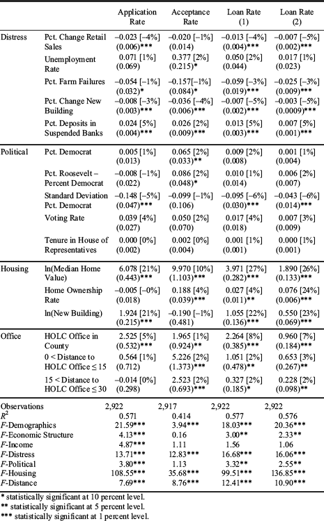
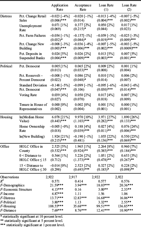
We present the results in Table 3. To conserve space, we only present the individual coefficient estimates for the distress, political, housing, and office variables and report the complete regression results in Appendix Table 2 of the online appendix. We do report, however, F-statistics for the joint significance of all the different categories of covariates at the bottom of the table. Besides reporting coefficient estimates and standard errors for individual covariates, we also show (in brackets) the percentage impacts on the dependent variables of one-standard-deviation increases in the independent variables to help assess economic significance.Footnote ³⁷

It is useful to begin by using the group F-statistics to characterize how the different categories of covariates influenced application, acceptance, and overall loan rates. The three groups of covariates not shown individually in the table—demographic, economic structure and income—all explain more of the variation in application rates than in acceptance rates, while the first two groups also explain significant variation in the two measures of loan rates. Among the covariate groups reported individually in the table, a similar pattern of influence appears only for the political variables which as a group explain application and loan rates, but not acceptance rates. The distress, housing, and distance variables, on the other hand, explain substantial variation in both loan rates and in the application and acceptance rates. These latter groups of variables have been chosen to reflect the structure of local housing markets, and the distress and lending costs faced by borrowers and lenders within them. Their combined importance in explaining HOLC activity provides strong evidence that the staff, borrowers, and lenders all broadly understood the goals and limits of the program.

TABLE 3

DETERMINANTS OF HOLC LOAN ACTIVITY

* statistically significant at 10 percent level.

** statistically significant at 5 percent level.

*** statistically significant at 1 percent level.

Notes:

Coefficient estimates, heteroskedasticity-robust standard errors (in parentheses), and percentage impacts of one-standard-deviation increases (in brackets) are reported. State fixed effects are included in all regressions. Results for the individual demographic, economic structure and income variables are available in Appendix Table 2 of the online appendix.

Three of the five individual distress covariates show the same consistent pattern of influence across applications, acceptances, and loan rates. Two of these, the percentage change in residential building activity and the percent of suspended bank deposits, are key measures that we use here to capture the disruption in local housing and financial markets. The coefficient estimates for both of these variables are of the expected sign, and the magnitude of their impacts are large enough to conclude that HOLC lending activity was sensitive to the distress and disruptions that the program was intended to combat. Increased incidence of farm failures has a modest negative impact on all rates, which could reflect a greater reliance in these areas on the New Deal's Farm Credit Administration.Footnote ³⁸ The two more generic measures of economic distress in our specification perform less consistently. The percentage change in retail sales has the expected, and statistically significant, negative association with application rates, but not with the rate of HOLC acceptances. The unemployment rate, on the other hand, has virtually no impact on any measure of HOLC activity.

We interpret the large and significant impacts for all of the individual housing covariates as evidence that the pattern of HOLC refinancing was related not only to distress, but also to its eligibility requirements. Markets in which median home values were higher in 1930 had higher rates of both applications and acceptances, presumably because high pre-crisis values indicated a more extensive reliance on mortgages and stronger post-crisis collateral.Footnote ³⁹ According to the percentage impact calculations, in fact, median home value has the strongest effect of all of the independent variables in every regression. The large positive effect of the volume of new homes built between 1925 and 1929 on county-level application rates also comports with evidence that new homes were more likely to have been under mortgage and eligible for refinancing.Footnote ⁴⁰ Finally, the statistically significant, positive and large impact of the homeownership rate on acceptance rates is consistent with C. Lowell Harriss' observation that HOLC set appraisals more favorably on properties located in settled, established residential areas than those in mixed, transitional neighborhoods.Footnote ⁴¹

Against this backdrop, the regressions provide little evidence that HOLC was driven to any appreciable degree by political considerations. Two of the five political variables in our specification (voting rate and tenure in the House) have no statistically significant association with any of our measures of HOLC activity. Two other political variables, the shares of Democratic and Roosevelt votes in 1932, are positively associated with slightly higher acceptance rates but are not significantly related to either overall loan rate. The only significant impact of political considerations on overall loan rates is through the association between stronger party loyalty, as measured by the standard deviation of percent Democrat, and application rates—but the variable has no impact on acceptance rates. Most importantly, the small share of the overall variability in application, acceptance, and loan rates that is explained by political considerations (refer to the F-statistics) represents evidence that HOLC was not in any important sense an instrument of patronage.

We close the discussion of HOLC allocation by focusing on the results for the HOLC office location variables separately, as they will prove crucial to the identification of the agency's impact in the next section. Having an HOLC office increases a county's application, acceptance, and loan rates. Interestingly, though, the nearest loan office being outside the county but less than 15 miles away or between 15 and 30 miles away matters to acceptance and loan rates but not to application rate.Footnote ⁴² This result is important and interesting for two reasons. First, it indicates that spatial segmentation in the mortgage market of lending operated more through supply than demand—because the costs to HOLC of conducting on-site appraisals and filing loan documents were greater for loans made in distant locales while most applications for relief were submitted by mail and thus not sensitive to distance to an office. Second, the effect of these costs had on HOLC treatment levels is plausibly exogenous and provides an avenue through which we can identify the consequence of HOLC loan activity for local housing outcomes.Footnote ⁴³

HOLC'S INTERVENTION AND THE LOCAL HOUSING MARKETS

We next turn to an evaluation of the effectiveness of HOLC. An OLS estimator of the relationship between percentage of homes refinanced by HOLC and housing market outcomes would likely be biased downward since the agency's loans were distributed disproportionately to areas facing the greatest housing and overall distress, as shown in the preceding section. We therefore estimate HOLC's impact with two-stage instrumental variables models in which the first stage predicts treatment intensity using an equation similar to equation 1 and the second examines the relationship between treatment intensity and 1940 nonfarm home values and ownership rates, as well as the number of new nonfarm housing units built in each county between 1935 and 1940. Identification requires one or more independent variables that meet the two criteria for valid instruments: they must affect HOLC loan rate in the first stage, and they must be uncorrelated with the second-stage error term that reflects unobserved characteristics that impacted housing markets during the 1930s.

Our identification strategy exploits the plausibly exogenous variation in loan activity resulting from the spatial configuration of HOLC's administration. Our earlier results showed that HOLC acceptance and loan rates decreased with the distance between a county and the nearest HOLC office, so the three office variables are likely to satisfy the first condition for valid instruments. The second condition is potentially more problematic. HOLC administrators naturally placed offices in large cities, and housing markets in large urban areas generally suffered the most during the Great Depression.Footnote ⁴⁴ Even conditional on population, HOLC administrators could have deliberately placed offices in the most troubled areas in an effort to best meet the needs of homeowners and lenders. Either phenomenon could lead to a downward bias when using all three office variables as instruments.

Fortunately, our indicator of nonfarm housing market distress—percentage change in new building during the early stages of the Depression—allows us to directly test whether HOLC offices were in fact placed in the most distressed areas. We begin by computing correlations between percentage change in new building from 1925–1929 to 1930–1934 and each of the three distance from HOLC office variables. The correlation between percentage change in new building and whether the county contains an office is −0.22 and significant at the 0.01 percent level, a result that is not surprising given the discussion above. Interestingly, however, the correlations between the change in building and the other two office variables are much smaller: −0.04 and significant at the 5 percent level for the indicator of whether the nearest office was outside the county but within 15 miles, and a statistically insignificant −0.01 for whether the nearest office was 15 to 30 miles away.

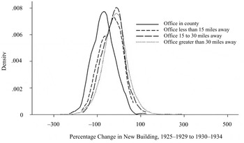
To investigate these patterns more closely, in Figure 1 we display kernel density functions for percentage change in new building, stratified by nearest HOLC office location. These plots reveal a similar story. The kernel density function for counties with an office lies well to the left of the function for the “control group” of counties whose nearest office is more than 30 miles away. The kernel density functions for counties whose nearest office is less than 15 miles away and those whose nearest office is 15 to 30 miles away, however, are similar to that of the control group in shape and value at which the function is maximized.Footnote ⁴⁵ The correlations and kernel density plots therefore suggest that HOLC indeed opened offices in counties facing the most housing market distress, but that the degree to which this relationship spilled over into surrounding areas was minimal.Footnote ⁴⁶ Consequently, the under 15 and 15–30 mile groups are the most appropriate comparison groups for the over 30 mile control group, while the counties containing an office are not an appropriate comparison group.

FIGURE 1

KERNEL DENSITY PLOTS OF PERCENTAGE CHANGE IN NEW BUILDING BY DISTANCE FROM HOLC OFFICE CATEGORY

Sources: Author's calculations. See the text.

With this in mind, we estimate two instrumental variables models using two-stage least squares. In both, the first stage regression is

(2)

The two second-stage regressions are

(3)

(4)

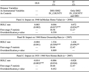
where equation 3 excludes the under 15 and 15–30 mile distance variables (DIS1 and DIS2) as instruments but keeps the variable for whether there is an office in the county (IN_COUNTY) as a control, while equation 4 excludes DIS2 as an instrument and keeps IN_COUNTY and DIS1 as controls.Footnote ⁴⁷ In this section, HOLC represents the percentage of nonfarm housing units refinanced with HOLC loans in each county. This is the dependent variable from the preceding section that best measures the extent to which a county was “treated” by the program. The second-stage dependent variable Y is the natural logarithm of nonfarm median home value, the nonfarm home ownership rate, or the natural logarithm of nonfarm new housing units built from 1935 to 1940. Since HOUS includes 1930 home values and ownership rates and new building in 1925–1929, the second stage is a lagged dependent variable model that corrects for time-invariant sources of endogeneity bias.Footnote ⁴⁸ We include the changes in the demographic and economic structure variables between 1930 and 1940 (represented by ΔDEMO and ΔECON) since the outcome variables in the second-stage regression are measured in 1940. We do not include changes in the other independent variables, such as the income and distress measures, since their values in 1940 are potentially functions of HOLC treatment.Footnote ⁴⁹ We omit state fixed effects for now to allow the substantial between-state variation in the number of offices that resulted from the states' autonomy in administering the program to increase the explanatory power of our instruments.Footnote ⁵⁰ We add them later as a robustness check.

In equation 3, the parameter of interest γ₁ is identified under the assumption that distance from the nearest HOLC office is uncorrelated with unobservable characteristics that impacted housing markets during the 1930s conditional on the county not having an office. In equation 4, the identifying assumption is that distance from the nearest office is uncorrelated with these unobservable characteristics conditional on there not being an office within 15 miles. We also considered using all three office variables as instruments but found that using IN_COUNTY as an instrument appears to bias the coefficient estimator for HOLC downward in the values and ownership regressions. This pattern is consistent with the correlations and kernel density plots discussed above.

Table 4 reports the results for each of the three dependent variables. The column labeled OLS displays the results from an OLS version of equation 3, while the columns labeled IV (1) and IV (2) represent the two aforementioned instrumental variables models. We display the coefficient estimates for HOLC loan rate in the second stage. When applicable, we also report the Kleibergen-Paap F-statistic from a test of the joint significance of the instruments in the first stage, along with the p-value from the overidentification test.

Panel A of Table 4 displays the results for median home values. In the OLS regression, HOLC loan rate is statistically insignificant and its effect is minimal. In both IV regressions, loan rate becomes statistically significant while the coefficient estimate reaches a magnitude (7.2–8.6 percent) that implies the median home value in the average county increased by 19–22 percent for an additional standard deviation increase in HOLC lending. The models reported in Panel B reveal a similar pattern for HOLC's impact on home ownership—the estimated coefficient is essentially zero using OLS, but large and statistically significant in both IV regressions. A one percentage point increase in the HOLC loan rate is associated with a 1.4–1.5 percentage point increase in the home ownership rate, meaning that HOLC actually preserved more than one homeowner for every home that it refinanced. These estimates imply that an additional standard deviation of HOLC lending increased the average county's home ownership rate by 3.6–3.9 percentage points. For both values and ownership rates, Hausman tests (not reported) reject the consistency of the OLS estimator and confirm our suspicion that it suffers from a downward bias. Both overidentification tests fail to reject the null hypothesis that DIS1 and DIS2 are valid instruments. The first-stage F-statistics are virtually identical in the two sets of regressions, differing only because of the slightly larger sample size for homeownership. They are large enough to rule out weak instrument bias using a maximum acceptable bias of 20 percent in IV (1) and 15 percent in IV (2).

Panel C shows HOLC's estimated impact on the volume of new homebuilding between 1935 and 1940. HOLC lending is associated with a statistically significant reduction in building in the OLS regression, but the magnitude is small. A one percentage point increase in loan rate is associated with a 1.3 percent reduction in new building, which would translate to only a 0.16 percent reduction in overall housing stock based on the sample means of the new building variable and the number of housing units. In both IV regressions, loan rate becomes insignificant and its effect remains small. The evidence is therefore consistent with HOLC having a minimal effect on housing production. Since all three estimates are close to zero, neither the Hausman nor overidentification tests reject the null hypothesis. The first-stage F-statistics are identical to those for homeownership rates as the sample is the same.

TABLE 4

EFFECTS OF HOLC LOAN ACTIVITY

* statistically significant at the 10 percent level.

** statistically significant at the 5 percent level.

*** statistically significant at the 1 percent level.

Notes:

Heteroskedasticity-robust standard errors in parentheses. All regressions include the demographic, economic structure, distress, political, and housing controls as well as the changes in the demographic and economic structure variables between 1930 and 1940. IV (1) corresponds to equation 3 in the text and IV (2) corresponds to equation 4.

We tested the sensitivity of the IV results by performing a wide range of robustness checks that are reported in Appendix Table 3 of the online appendix. First, we included additional controls that measure per capita spending on five New Deal programs besides HOLC, state fixed effects, and changes in the dependent variables within the farm portion of each county during the 1930s.Footnote ⁵¹ We also employed different methods of measuring distance from the nearest HOLC office: three 10-mile distance dummies instead of two 15-mile dummies, a single 30-mile distance dummy plus the interaction of this dummy with linear distance and the distance from July 1935, instead of January 1934, office locations. Additional models incorporated more flexible specifications for the important population, population density, and percent urban control variables, while others used different measures of HOLC treatment intensity—the proportion of owned (instead of all) homes that were refinanced and a per capita dollar measure of lending in each county. We also use levels rather than logs of median home values and new home construction, and weight each county by the natural logs of population and nonfarm housing units. Finally, we consider models that restrict the sample to counties that did not contain an HOLC office and those that did not have an HOLC office within 15 miles. Our central result that HOLC lending increased home values and ownership rates, but not new building, persists throughout all of these specifications.

Heterogeneity

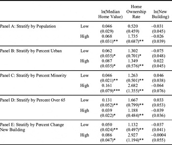
Thus far our analysis of HOLC's impact on local housing markets has focused on identifying average effects. A particular amount of HOLC lending could have had different effects in different housing markets, however, because the severity of disruptions in mortgage lending channels would have depended on the institutional and contractual elements used in each market, while the impacts of the disruptions would have varied across different categories of mortgaged homeowners. To examine whether HOLC effects were heterogeneous, we split the sample into two subsamples based on population, percent urban, percent minority (race other than white), percent over 65 years old, and percent change in new building between 1925–1929 and 1930–1934.Footnote ⁵² We constructed subsamples by first dropping the 209 counties that contained HOLC offices—as they are not used for identification in our IV specifications—and then splitting the remaining 2,698 counties into those above and below the median along the selected dimension. We then conducted IV estimation with DIS1 and DIS2 as instruments.

TABLE 5

HETEROGENEITY

* statistically significant at the 10 percent level.

** statistically significant at the 5 percent level.

*** statistically significant at the 1 percent level.

Notes:

Heteroskedasticity-robust standard errors in parentheses. All regressions include the demographic, economic structure, distress, political, and housing controls as well as the changes in the demographic and economic structure variables between 1930 and 1940.

Table 5 reports the results, with “low” and “high” indicating the halves of the sample below and above the sample median. The impact of HOLC on home values and ownership rates appears to have been strongest in large, urban areas with a diverse and young population. This result could indicate that younger homeowners, who tend to stretch financially when purchasing a home, benefitted disproportionately by HOLC refinancing since they had less wealth than older homeowners to absorb the shocks associated with disruptions in income. Interestingly, HOLC also appears to have had the greatest effect in the half of the counties facing the lower amounts of housing market distress. This could indicate that HOLC was effective so long as mortgage disruptions were not too severe—but beyond some point even HOLC loans could not ameliorate the damage.

Artificial Offices, Large Urban Markets, and Identifying the Impacts of the HOLC

We close our analysis with an effort to tie our results together with those of Fishback et al. to provide a clear picture of what we have and have not learned about the effects of HOLC on local housing markets during the Great Depression. Like us, Fishback et al. exploit distance from HOLC offices in their identification strategy and recognize the potential endogeneity of these office locations. Whereas we account for this potential endogeneity by controlling for whether the county has an office, their proposed solution is to use “artificial” instead of actual office locations. Noting that HOLC offices were typically placed in large cities, they place an artificial office in each state's capital and the four most heavily populated counties, and then create the instrument by computing distances from these artificial locations. Constructing artificial office locations using pre-Depression characteristics such as size should indeed correct for bias from HOLC administrators deliberately placing offices in counties facing the greatest housing market distress. But their approach is still susceptible to bias from large counties experiencing different housing market shocks than other areas in the 1930s for reasons aside from HOLC. The other controls should mitigate the extent of this bias, but may not eliminate it completely.

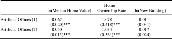
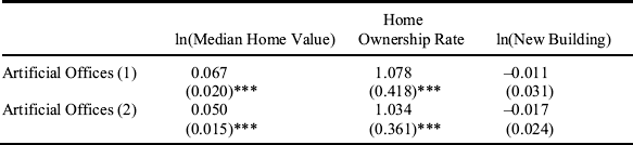
To better understand how the identification issue can change our view of HOLC's impacts, in this section we consider two variations of the artificial HOLC office approach. The first specification (referred to as “Artificial Offices 1”) duplicates the artificial office locations used by Fishback et al.: each state's capital and four largest counties. The second specification (“Artificial Offices 2”) offers our own method of constructing artificial office locations. We first estimate a probit model with IN_COUNTY as the dependent variable and county characteristics from 1920—before both the 1920s boom and 1930s bust—as the independent variables. These 1920 variables include the set of demographic characteristics plus dummy variables for the state capital and the five most heavily populated counties in the state. We then assign offices to the 209 counties with the highest predicted probabilities, subject to the constraint that every state has at least one office. This method correctly predicts 147 of the 209 actual office locations, while Fishback et al.'s artificial office approach correctly predicts 138. We then construct distances from the nearest artificial HOLC office, using the same divisions as before: in the county, outside the county but within 15 miles, between 15–30 miles, and beyond 30 miles.

As with actual offices, we can assess the validity of these artificial office approaches by examining the relationship between our set of distance-from-office variables and our measure of nonfarm housing market distress—the percentage change in new building from 1925–1929 to 1930–1934. Using “Artificial Offices 1,” the correlation between IN_COUNTY and percentage change in new building from 1925–1929 to 1930–1934 is −0.19 and significant at the 0.01 percent level. The correlations between change in new building and DIS1 and DIS2, however, are both only −0.03 and insignificant at the 5 percent level. Using “Artificial Offices 2,” the correlation between change in new building and IN_COUNTY is a significant −0.24, while the correlations between change in new building and DIS1 and DIS2 are both an insignificant −0.03. Accordingly, the kernel density plots in Appendix Figures 1 and 2 of the online appendix both show that the distress distribution for counties with an artificial office lies to the left of the distributions for the other three groups of counties. These patterns point to the same conclusion reached with actual offices: relative to the “control group” of counties whose nearest artificial HOLC office is more than 30 miles away, counties whose nearest artificial office is within 15 miles (but not in the county) or 15–30 miles away are more appropriate comparison groups than counties that contain an artificial office.

Table 6 displays the results from the artificial offices regressions utilizing both DIS1 and DIS2 as instruments and IN_COUNTY as a control.Footnote ⁵³ As with actual offices, HOLC lending has a statistically and economically significant impact on median home values and ownership rates but no effect on new building. The magnitudes of the estimates are slightly smaller but well within the 95 percent confidence intervals of those obtained using actual offices.

TABLE 6

ARTIFICIAL OFFICES

Notes:

See the notes for Table 5.

Our results can now be combined with those of Fishback et al. to assess what we know and do not know about HOLC's role in stabilizing home values and home ownership. Importantly, both papers agree that HOLC increased housing values and home ownership (stock of owned homes in their case, ownership rate in ours) once the few hundred largest counties are excluded from the sources of identifying variation.Footnote ⁵⁴ The evidence therefore indicates that HOLC successfully repaired credit channels and prevented further disruptions in the housing and mortgage markets across most of the nation's counties. HOLC's effectiveness in the largest counties, however, is less clear. Fishback et al. noted that keeping counties with over 50,000 residents in the sample weakened HOLC's estimated impacts dramatically and conjectured that this result was due to heterogeneity in impacts between the largest counties and all other markets in the sample. We argue, in contrast, that the distance-based instrumental variable approach is simply not appropriate to identify HOLC's impacts within the largest counties because these markets hosted disproportionate numbers of actual or artificial offices while facing the greatest housing market distress in the early stages of the Depression.

These differences in interpretation point to the need for future research to examine HOLC's intervention in the largest counties. The issue matters because these markets took the brunt of the real estate crisis in terms of average decreases in home values, homeownership rates and housing production—and also received a disproportionately large share of HOLC funds.Footnote ⁵⁵