1 Introduction
Inertia–gravity waves are known to be a significant mechanism for energy and momentum transfer in the ocean and atmosphere (Sutherland Reference Sutherland2010). While a substantial amount of progress in understanding of their roles has been achieved via plane wave models, a planar geometry is not necessarily appropriate for studies pertaining to natural phenomena such as oceanic internal wave generation by hurricanes (Kumar, Ramkumar & Krishnaiah Reference Kumar, Ramkumar and Krishnaiah2011) and tropical cyclones (Schubert et al. Reference Schubert, Hack, Silva Dias and Fulton1980), and atmospheric generation by thunderstorms (Sentman et al. Reference Sentman, Wescott, Picard, Winick, Stenbaeck-Nielsen, Dewan, Moudry, São Sabbas, Heavner and Morrill2003). Furthermore, Warren (Reference Warren1960) noted that a vertical disturbance of small spatial extent compared to the horizontal dimension of the system in a stably stratified fluid like the atmosphere leads to the emission of an axisymmetric perturbation. As such, axisymmetry is a reasonable approximation to consider for inertia–gravity waves generated by localised disturbances in either the atmosphere or the ocean.
Mowbray & Rarity (Reference Mowbray and Rarity1967) and Appleby & Crighton (Reference Appleby and Crighton1987) studied immersed objects such as spheres as being sources of radiated axisymmetric internal waves. Several subsequent laboratory experimental studies investigated axisymmetric inertia–gravity waves, focusing primarily on the global structure of the cone-shaped internal wave emission induced by an oscillating or rotating object (Peacock & Weidman Reference Peacock and Weidman2005; Duran-Matute et al. Reference Duran-Matute, Flór, Godeberd and Jause-Labert2013; Ghaemsaidi & Peacock Reference Ghaemsaidi and Peacock2013; Le Dizès Reference Le Dizès2015). More recently, Ansong & Sutherland (Reference Ansong and Sutherland2010) investigated internal waves excited by an axisymmetric convective plume in a constant density-gradient stratification, and Brandt & Shipley (Reference Brandt and Shipley2019) performed experiments of internal wave generation with an axisymmetric plume in a two-layer stratification, one of them being of constant density. To obtain a high degree of control on the spatial form of an axisymmetric source, Maurer et al. (Reference Maurer, Ghaemsaidi, Joubaud, Peacock and Odier2017) adapted the oscillating plate planar generator of Gostiaux et al. (Reference Gostiaux, Didelle, Mercier and Dauxois2006) to produce a wave generator capable of producing axisymmetric internal wave fields of arbitrary radial form, such as truncated Bessel modes or annular patterns, which opens the door on a wide range of possible experimental investigations. Inspired by studies on confined two-dimensional internal waves, Boury, Peacock & Odier (Reference Boury, Peacock and Odier2019) used this apparatus to produce pure axisymmetric modes that can be used as the basis for understanding the behaviour of more complex fields via modal decomposition using the natural cylindrical basis of Bessel functions.
In the oceans and atmosphere an important consideration is the vertical form of the density gradient, as shown in the works of King et al. (Reference King, Stone, Zhang, Gerkema, Marder, Scott and Swinney2012) and Paoletti & Swinney (Reference Paoletti and Swinney2012) with numerical and in situ studies of an exponentially decaying buoyancy frequency. The influence of non-uniform stratifications has been studied for a planar geometry, determining transmission and reflection coefficients for stratifications with sharp (Nault & Sutherland Reference Nault and Sutherland2007; Mathur & Peacock Reference Mathur and Peacock2009) and smooth (Brown & Sutherland Reference Brown and Sutherland2007; Mathur & Peacock Reference Mathur and Peacock2009) discontinuities. Numerical and experimental studies show good agreement with the theoretical predictions, considering two different scenarios: one with freely propagating incident waves (Sutherland & Yewchuk Reference Sutherland and Yewchuk2004; Mathur & Peacock Reference Mathur and Peacock2009), a configuration relevant to the atmosphere, and another with parametric subharmonic instability in a forced, upper stratification layer (Ghaemsaidi et al. Reference Ghaemsaidi, Dosser, Rainville and Peacock2016), relevant to an ocean configuration. In the latter case, the finite extent of the upper layer leads to interference between downward and upward waves reflected at the top and bottom boundaries (Mathur & Peacock Reference Mathur and Peacock2010), a phenomenon similar to resonant cavities in optics (Perot & Fabry Reference Perot and Fabry1899) or Helmholtz cavities for sound waves (Rayleigh Reference Rayleigh1945; Morse Reference Morse1948). Such a resonant behaviour – by which we mean constructive interference – has been observed by Sutherland & Yewchuk (Reference Sutherland and Yewchuk2004) and has been proven capable of triggering high amplitude wave fields (Boury et al. Reference Boury, Peacock and Odier2019).
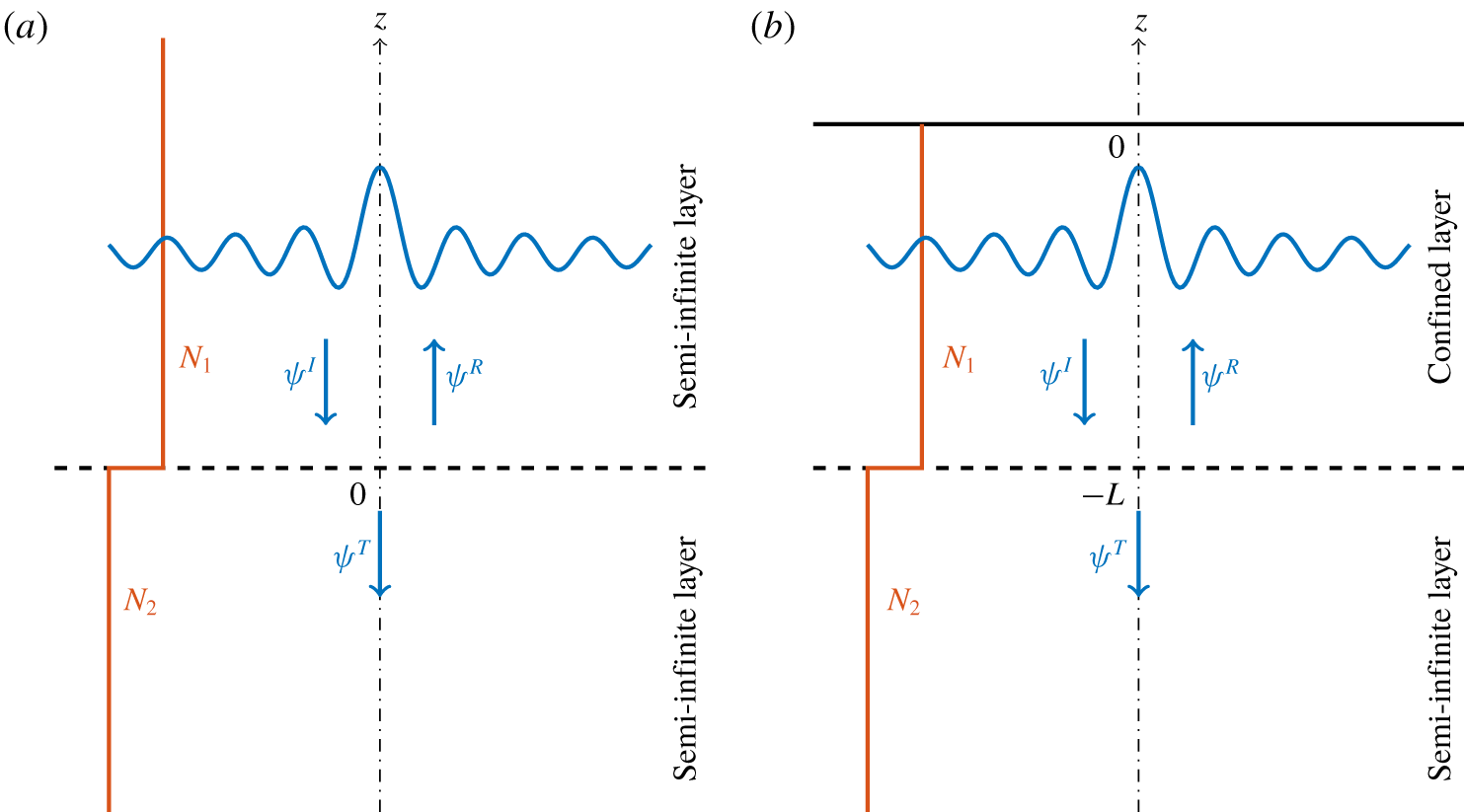
To date, all experimental studies of axisymmetric internal wave fields have considered linearly stratified fluids, or stratifications with transitions between a linear stratified fluid and an unstratified layer (Ansong & Sutherland Reference Ansong and Sutherland2010; Brandt & Shipley Reference Brandt and Shipley2019), and there have been no such transmission studies for axisymmetric inertia–gravity wave fields involving two layers of different non-zero buoyancy frequency. In this paper, therefore, we delve further into the propagation properties of axisymmetric internal waves in nonlinear stratifications. The plane wave analysis of Mathur & Peacock (Reference Mathur and Peacock2009) is extended to cylindrical wave modes and we derive a theoretical prediction for their transmission across a buoyancy frequency interface. Using the experimental configuration of Boury et al. (Reference Boury, Peacock and Odier2019), experimental transmission studies are conducted for a freely propagating axisymmetric internal wave and for an axisymmetric internal wave field excited in an upper layer (see figure 1); in both cases the radial form of the wave field is a mode 1 Bessel function. In § 2, we derive the theoretical framework and define the boundary value problem used for numerical computation. Then, in § 3, we describe the experimental apparatus. Our experimental results are presented in § 4, followed by oceanographic considerations in § 5 and conclusions and discussion in § 6.
2 Theory
2.1 Governing equations
Transmission of a radial mode  $J_{1}$ across a buoyancy frequency interface. The
 $z$ axis is located at
 $r=0$. In both cases, the interface is modelled by a sharp discontinuity in buoyancy frequency, and the blue pattern represents a Bessel shaped wave field. (a) Free incident wave
 $\unicode[STIX]{x1D713}^{I}$ reaching the interface, leading to a reflected wave
 $\unicode[STIX]{x1D713}^{R}$ and a transmitted wave
 $\unicode[STIX]{x1D713}^{T}$. (b) A confined incident wave
 $\unicode[STIX]{x1D713}^{I}$, located between the surface at
 $z=0$ and the interface at
 $z=-L$, is an infinite sum of waves being reflected at
 $z=0$ and at
 $z=-L$, and leads to a transmitted wave
 $\unicode[STIX]{x1D713}^{T}$.

Focusing on an inviscid Boussinesq fluid rotating at an angular velocity  $\unicode[STIX]{x1D6FA}$, with a density stratification
 $\unicode[STIX]{x1D70C}(z)$ where
 $z$ is the ascendant vertical, small amplitude internal waves satisfy the following equation in cylindrical coordinates (Boury et al. Reference Boury, Peacock and Odier2019; Maurer et al. Reference Maurer, Ghaemsaidi, Joubaud, Peacock and Odier2017)
 $$\begin{eqnarray}{\displaystyle \frac{\unicode[STIX]{x2202}^{2}}{\unicode[STIX]{x2202}t^{2}}}\left({\displaystyle \frac{\unicode[STIX]{x2202}^{2}\unicode[STIX]{x1D713}}{\unicode[STIX]{x2202}z^{2}}}+{\displaystyle \frac{\unicode[STIX]{x2202}}{\unicode[STIX]{x2202}r}}\left(\frac{1}{r}{\displaystyle \frac{\unicode[STIX]{x2202}(r\unicode[STIX]{x1D713})}{\unicode[STIX]{x2202}r}}\right)\right)=-f^{2}{\displaystyle \frac{\unicode[STIX]{x2202}^{2}\unicode[STIX]{x1D713}}{\unicode[STIX]{x2202}z^{2}}}-N^{2}{\displaystyle \frac{\unicode[STIX]{x2202}}{\unicode[STIX]{x2202}r}}\left(\frac{1}{r}{\displaystyle \frac{\unicode[STIX]{x2202}(r\unicode[STIX]{x1D713})}{\unicode[STIX]{x2202}r}}\right),\end{eqnarray}$$
in which  $f=2\unicode[STIX]{x1D6FA}$ is the Coriolis frequency, and
 $N=\sqrt{(-g/\unicode[STIX]{x1D70C}_{0})\unicode[STIX]{x2202}\bar{\unicode[STIX]{x1D70C}}/\unicode[STIX]{x2202}z}$ is the buoyancy frequency,
 $\unicode[STIX]{x1D70C}_{0}$ being the reference density. The streamfunction
 $\unicode[STIX]{x1D713}$ is defined so that the radial and vertical velocities
 $v_{r}$ and
 $v_{z}$ are
 $$\begin{eqnarray}v_{r}=-\frac{1}{r}{\displaystyle \frac{\unicode[STIX]{x2202}(r\unicode[STIX]{x1D713})}{\unicode[STIX]{x2202}z}}\quad \text{and}\quad v_{z}=\frac{1}{r}{\displaystyle \frac{\unicode[STIX]{x2202}(r\unicode[STIX]{x1D713})}{\unicode[STIX]{x2202}r}}.\end{eqnarray}$$
In the configuration of a horizontal forcing in a linear stratification ( $N$ is a constant), the solutions of (2.1) can be expressed as a product of two decoupled functions: a radial part depending on the radius
 $r$, and a vertical part depending on the depth
 $z$. The cylindrical geometry leads to a natural decomposition over Bessel functions for the radial component and exponentials for the vertical component. Using a complex notation, the streamfunction can therefore be written as a sum of cylindrical modes of the form (Boury et al. Reference Boury, Peacock and Odier2019)
 $$\begin{eqnarray}\unicode[STIX]{x1D713}(r,z,t)=\unicode[STIX]{x1D713}_{0}J_{1}(lr)\text{e}^{\text{i}(mz-\unicode[STIX]{x1D714}t)},\end{eqnarray}$$
with  $\unicode[STIX]{x1D713}_{0}$ a constant amplitude,
 $\unicode[STIX]{x1D714}$ the wave frequency and
 $l$ and
 $m$ its radial and vertical wavenumbers. The radial dependence is expressed through a first-order Bessel function of the first kind
 $J_{1}$, corresponding to a non-divergent mode. In the case of either a free propagating or evanescent wave, the vertical dependence can be written with an exponential. For a more general framework in further sections, for example while considering vertically confined wave fields, the vertical component will be noted
 $\unicode[STIX]{x1D719}$. As in a Cartesian geometry, the parameters
 $\unicode[STIX]{x1D714}$,
 $l$ and
 $m$ are linked through the internal wave dispersion relation (Maurer et al. Reference Maurer, Ghaemsaidi, Joubaud, Peacock and Odier2017; Boury et al. Reference Boury, Peacock and Odier2019)
 $$\begin{eqnarray}m=\pm l\left(\frac{\unicode[STIX]{x1D714}^{2}-N^{2}}{f^{2}-\unicode[STIX]{x1D714}^{2}}\right)^{1/2},\end{eqnarray}$$
derived from (2.1), (2.2) and (2.3).
In the next two sections, we discuss the two scenarios presented in figure 1, initially assuming a sharp interface (discontinuity between two different buoyancy frequencies  $N_{1}$ and
 $N_{2}$, with
 $N_{1}>N_{2}$). Figure 1(a) shows the transmission of a free incident wave
 $\unicode[STIX]{x1D713}^{I}$, which is more relevant to the modelling of atmospheric internal waves, whereas figure 1(b) shows the transmission of an incident wave confined from above, which is closer to an oceanic situation with a surface forcing.
2.2 Transmission of a free incident wave
2.2.1 Sharp interface
Linear vertical propagation of radial modes has been extensively studied by Boury et al. (Reference Boury, Peacock and Odier2019). In this section, we consider a horizontal interface located at  $z=0$ that splits the domain into two media of constant buoyancy frequency
 $N$:
 $N_{1}$ in the upper layer (
 $z>0$),
 $N_{2}$ in the lower layer (
 $z<0$), the density being continuous at the interface (figure 1a). We assume a larger buoyancy frequency in the upper layer so that
 $N_{1}>N_{2}$. As depicted in figure 1(a), a free incident wave
 $\unicode[STIX]{x1D713}^{I}$ reaching the interface leads to a reflected wave
 $\unicode[STIX]{x1D713}^{R}$ in the upper region, and a transmitted wave
 $\unicode[STIX]{x1D713}^{T}$ in the lower region. The total wave field can be described by
 $\unicode[STIX]{x1D713}_{1}=\unicode[STIX]{x1D713}^{I}+\unicode[STIX]{x1D713}^{R}$ in the upper region, where
 $\unicode[STIX]{x1D713}^{I}$ is known, and by
 $\unicode[STIX]{x1D713}_{2}=\unicode[STIX]{x1D713}^{T}$ in the lower region.
We define the transmission coefficients as the ratios of the velocities above and under the interface, as
 $$\begin{eqnarray}T_{v_{z}}=\left|\frac{v_{z}^{T}}{v_{z}^{I}}\right|\quad \text{and}\quad T_{v_{r}}=\left|\frac{v_{r}^{T}}{v_{r}^{I}}\right|,\end{eqnarray}$$
and
 $$\begin{eqnarray}R_{v_{z}}=\left|\frac{v_{z}^{R}}{v_{z}^{I}}\right|\quad \text{and}\quad R_{v_{r}}=\left|\frac{v_{r}^{R}}{v_{r}^{I}}\right|,\end{eqnarray}$$
where the notation  $I$,
 $R$ and
 $T$, indicates that the vertical velocity
 $v_{z}$ or the radial velocity
 $v_{r}$ is computed from the streamfunctions
 $\unicode[STIX]{x1D713}^{I}$,
 $\unicode[STIX]{x1D713}^{R}$ and
 $\unicode[STIX]{x1D713}^{T}$, respectively (see figure 1). These velocities are taken at the interface, which means in the limit
 $z\rightarrow 0$.
Transmission and reflection properties can be derived by applying boundary conditions at the interface: continuity of the total vertical velocity field  $v_{z}$ and the pressure
 $p$ derived from
 $\unicode[STIX]{x1D713}_{1}$ and
 $\unicode[STIX]{x1D713}_{2}$ (Mathur & Peacock Reference Mathur and Peacock2009). As in Cartesian geometry, these quantities can be obtained using the linearised Navier–Stokes equations (Ansong & Sutherland Reference Ansong and Sutherland2010). The transmission and reflection coefficients for the radial and vertical velocities
 $v_{r}$ and
 $v_{z}$, and the flux of the energy
 $j=pv_{z}$ across the interface, can therefore be derived, respectively, as
 $$\begin{eqnarray}T_{v_{r}}=\left|\frac{2m_{2}}{m_{1}+m_{2}}\right|,\quad T_{v_{z}}=\left|\frac{2m_{1}}{m_{1}+m_{2}}\right|,\quad \text{and}\quad T_{j}=\left|\frac{4m_{1}m_{2}}{(m_{1}+m_{2})^{2}}\right|,\end{eqnarray}$$
and
 $$\begin{eqnarray}R_{v_{r}}=\left|\frac{m_{1}-m_{2}}{m_{1}+m_{2}}\right|,\quad R_{v_{z}}=\left|\frac{m_{2}-m_{1}}{m_{1}+m_{2}}\right|,\quad \text{and}\quad R_{j}=\left|\frac{(m_{1}-m_{2})^{2}}{(m_{1}+m_{2})^{2}}\right|,\end{eqnarray}$$
where  $m_{1}$ and
 $m_{2}$ are the vertical wavenumbers corresponding to regions
 $1$ and
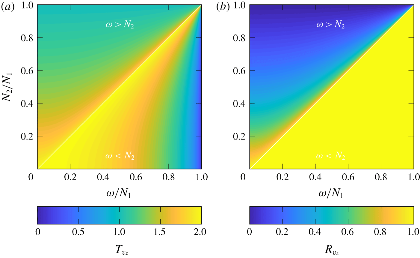
 $2$, given by the dispersion relation (2.4). These coefficients are the same as in a Cartesian geometry for a plane wave beam crossing a density-gradient interface (Mathur & Peacock Reference Mathur and Peacock2009), suggesting that the radial dependence does not affect wave properties at the interface although it still shapes the wave field and the energy distribution. Colour maps of the transmission and reflection coefficient for the vertical velocity,
 $T_{v_{z}}$ and
 $R_{v_{z}}$, are presented in figure 2 as functions of
 $N_{1}/N_{2}$ and
 $\unicode[STIX]{x1D714}/N_{1}$. A maximum of transmission of vertical velocity appears for
 $\unicode[STIX]{x1D714}/N_{1}=N_{2}/N_{1}$, when the wave just becomes evanescent in the lower region. This evanescence transition is clearly identified in the reflection coefficient, showing a total reflection of the wave field for
 $\unicode[STIX]{x1D714}/N_{1}>N_{2}/N_{1}$.
Colour maps of (a) the transmission coefficient  $T_{v_{z}}$ and (b) the reflection coefficient
 $R_{v_{z}}$ in vertical velocity, in the plane
 $(\unicode[STIX]{x1D714}/N_{1},N_{1}/N_{2})$. The Coriolis frequency is set to be
 $f=0$.

2.2.2 Smooth interface
Following the approach of Mathur & Peacock (Reference Mathur and Peacock2009), the propagation of the wave across a physical smooth interface of a finite-width transition region  $\unicode[STIX]{x1D6FF}$ is investigated using the buoyancy frequency profile
 $$\begin{eqnarray}N^{2}(z)=\left(\frac{N_{1}^{2}+N_{2}^{2}}{2}\right)+\left(\frac{N_{1}^{2}-N_{2}^{2}}{2}\right)\tanh \left(\frac{z}{\unicode[STIX]{x1D6FF}}\right),\end{eqnarray}$$
for which  $N$ is assumed to be constant far from the transition region and moves continuously from
 $N_{1}$ to
 $N_{2}$ at the interface located at
 $z=0$.
In a similar way to Mathur & Peacock (Reference Mathur and Peacock2009) and Nault & Sutherland (Reference Nault and Sutherland2007), the wave behaviour close to the interface is explored through a numerical approach. As the buoyancy frequency profile only depends on  $z$, the radial part is still described by a first-order Bessel function
 $J_{1}$. We use an ansatz describing the streamfunction as
 $$\begin{eqnarray}\unicode[STIX]{x1D713}(r,z,t)=\unicode[STIX]{x1D719}(z)J_{1}(lr)\text{e}^{\text{i}\unicode[STIX]{x1D714}t},\end{eqnarray}$$
where the vertical dependence is no longer described by an exponential as in (2.3) but by a  $z$-dependent function
 $\unicode[STIX]{x1D719}$. This function is found to satisfy the differential equation
 $$\begin{eqnarray}\unicode[STIX]{x1D719}^{\prime \prime }+\unicode[STIX]{x1D6FE}(z)\unicode[STIX]{x1D719}=0,\quad \text{with}~\unicode[STIX]{x1D6FE}(z)=l^{2}\left(\frac{\unicode[STIX]{x1D714}^{2}-N^{2}(z)}{f^{2}-\unicode[STIX]{x1D714}^{2}}\right),\end{eqnarray}$$
where  $\unicode[STIX]{x1D719}^{\prime \prime }$ stands for the second-order derivative of
 $\unicode[STIX]{x1D719}$, and
 $\unicode[STIX]{x1D6FE}$ is a function of
 $z$ that replaces the
 $m$ wavenumber given in the sharp interface study. Far from the interface, the wave field is expected to behave vertically as a Fourier mode, which implies an asymptotic form
 $$\begin{eqnarray}\tilde{\unicode[STIX]{x1D719}}(z)=\left\{\begin{array}{@{}ll@{}}\unicode[STIX]{x1D719}_{0}^{I}\text{e}^{\text{i}m_{1}z}+\unicode[STIX]{x1D719}_{0}^{R}\text{e}^{-\text{i}m_{1}z},\quad & \text{if}~z=z^{+},\\ \unicode[STIX]{x1D719}_{0}^{T}\text{e}^{\text{i}m_{2}z},\quad & \text{if}~z=z^{-},\end{array}\right.\end{eqnarray}$$
where  $\unicode[STIX]{x1D719}_{0}^{I}$,
 $\unicode[STIX]{x1D719}_{0}^{R}$ and
 $\unicode[STIX]{x1D719}_{0}^{T}$ are constants describing the amplitudes of the incoming, reflected and transmitted waves,
 $m_{1}$ and
 $m_{2}$ are the vertical wavelengths corresponding to the media of buoyancy frequencies
 $N_{1}$ and
 $N_{2}$ defined by (2.4) and
 $z^{+}$ and
 $z^{-}$ are two locations far from the interface respectively above and below it. The asymptotic expression
 $\tilde{\unicode[STIX]{x1D719}}$ can be written as boundary conditions for
 $\unicode[STIX]{x1D719}$:
 $$\begin{eqnarray}\displaystyle & \displaystyle \unicode[STIX]{x1D719}=\tilde{\unicode[STIX]{x1D719}},\quad \text{at }z=z^{+}, & \displaystyle\end{eqnarray}$$
 $$\begin{eqnarray}\displaystyle & \displaystyle \unicode[STIX]{x1D719}^{\prime }=\text{i}m_{2}\tilde{\unicode[STIX]{x1D719}},\quad \text{at }z=z^{-}. & \displaystyle\end{eqnarray}$$
 $z$-dependent function
 $\unicode[STIX]{x1D719}$ and allowing for the computation of the transmission and reflection coefficients.
2.2.3 Weakly viscous correction
As shown by Boury et al. (Reference Boury, Peacock and Odier2019), viscous damping for radial modes has to be considered while using frequencies such as  $\unicode[STIX]{x1D714}/N<0.5$. The weakly viscous correction can be described by assuming that the first-order correction in
 $\unicode[STIX]{x1D700}=\unicode[STIX]{x1D708}l^{2}/\unicode[STIX]{x1D714}$ for a vertical dependence of the streamfunctions as
 $\unicode[STIX]{x1D719}(z)\propto \text{e}^{\text{i}mz}$ takes the form (Boury et al. Reference Boury, Peacock and Odier2019)
 $$\begin{eqnarray}m=m^{(0)}+\text{i}\unicode[STIX]{x1D700}m^{(1)}+O(\unicode[STIX]{x1D700}^{2}),\end{eqnarray}$$
with  $m^{0}$ being the inviscid vertical wavenumber defined by (2.4), and
 $m^{1}$ the correction term:
 $$\begin{eqnarray}\text{i}\unicode[STIX]{x1D700}m^{(1)}=\mp \frac{\text{i}\unicode[STIX]{x1D700}l}{2(1-\unicode[STIX]{x1D6FE}^{2})\unicode[STIX]{x1D6FC}^{3}\sqrt{1-\unicode[STIX]{x1D6FC}^{2}}},\end{eqnarray}$$
where  $\unicode[STIX]{x1D6FC}=\unicode[STIX]{x1D714}/N$ and
 $\unicode[STIX]{x1D6FE}=f/\unicode[STIX]{x1D714}$. Hence, after propagating over a distance
 $z$, the weakly viscous streamfunction
 $\unicode[STIX]{x1D713}_{\unicode[STIX]{x1D708}}$ is written
 $$\begin{eqnarray}\unicode[STIX]{x1D713}_{\unicode[STIX]{x1D708}}(z)=\unicode[STIX]{x1D713}(z)\exp (-\unicode[STIX]{x1D700}m^{(1)}|z|).\end{eqnarray}$$
A more general calculation of the viscous correction, for arbitrary  $z$-dependent stratifications, can be found in Kistovich & Chashechkin (Reference Kistovich and Chashechkin1998).
Using the above expressions, the transmission coefficient can be computed numerically and compared to the inviscid case. The problem is solved as a boundary value problem, using a similar system as proposed before (2.13). Yet, as  $\unicode[STIX]{x1D719}$ is now driven by a fourth-order differential equation (Boury et al. Reference Boury, Peacock and Odier2019), the boundary value problem requires four conditions to be closed
 $$\begin{eqnarray}\displaystyle & \displaystyle \unicode[STIX]{x1D719}=\tilde{\unicode[STIX]{x1D719}},\quad \text{at }z=L, & \displaystyle\end{eqnarray}$$
 $$\begin{eqnarray}\displaystyle & \displaystyle \unicode[STIX]{x1D719}^{\prime \prime }=-(m_{1}^{(0)}+\unicode[STIX]{x1D700}m_{1}^{(1)})^{2}\tilde{\unicode[STIX]{x1D719}},\quad \text{at }z=L, & \displaystyle\end{eqnarray}$$
 $$\begin{eqnarray}\displaystyle & \displaystyle \unicode[STIX]{x1D719}^{\prime }=\text{i}(m_{2}^{(0)}+\unicode[STIX]{x1D700}m_{2}^{(1)})\tilde{\unicode[STIX]{x1D719}},\quad \text{at }z=z^{-}, & \displaystyle\end{eqnarray}$$
 $$\begin{eqnarray}\displaystyle & \displaystyle \unicode[STIX]{x1D719}^{\prime \prime }=-(m_{2}^{(0)}+\unicode[STIX]{x1D700}m_{2}^{(1)})^{2}\tilde{\unicode[STIX]{x1D719}},\quad \text{at }z=z^{-}. & \displaystyle\end{eqnarray}$$
2.3 Transmission of a confined incident wave
2.3.1 Sharp interface
In the previous section, semi-infinite domains were implicitly assumed. Such situations can be found in the atmosphere, as discontinuities in the buoyancy frequency profile are likely to be far from a source of internal waves. In the oceans, however, strong stratifications are often found close to the surface (Boury et al. Reference Boury, Peacock and Odier2019), so the upper layer cannot be modelled by a region that extends vertically without boundaries.
We therefore consider a sharp interface between  $N_{1}$ and
 $N_{2}$ at
 $z=-L$, and an upper rigid boundary (the ocean surface) at
 $z=0$, as presented in figure 1(b). Analytically, this problem can be solved as in the case of a semi-infinite domain, except that the boundary conditions are different because the incoming wave
 $\unicode[STIX]{x1D713}^{I}$ is not known. Instead, the total field at
 $z=-L$ is known and its vertical dependence satisfies:
 $\unicode[STIX]{x1D719}(z=-L)=\unicode[STIX]{x1D719}_{0}=\unicode[STIX]{x1D719}_{0}^{I}\text{e}^{-\text{i}Lm_{1}}+\unicode[STIX]{x1D719}_{0}^{R}\text{e}^{\text{i}Lm_{1}}$. The following transmission coefficients are derived using the same continuity properties at the interface as in the previous section:
 $$\begin{eqnarray}\displaystyle & \displaystyle T_{v_{r}}=\left|\frac{v_{r}^{T}}{v_{r}^{I}}\right|=\left|\left[\cos (Lm_{1})+\text{i}\left(\frac{m_{1}}{m_{2}}\right)\sin (Lm_{1})\right]^{-1}\right|, & \displaystyle\end{eqnarray}$$
 $$\begin{eqnarray}\displaystyle & \displaystyle T_{v_{z}}=\left|\frac{v_{z}^{T}}{v_{z}^{I}}\right|=\left|\left[\cos (Lm_{1})+\text{i}\left(\frac{m_{2}}{m_{1}}\right)\sin (Lm_{1})\right]^{-1}\right| & \displaystyle\end{eqnarray}$$
and
 $$\begin{eqnarray}\displaystyle T_{j}=\left|\left[\cos (2Lm_{1})+\text{i}\left(\frac{m_{1}^{2}+m_{2}^{2}}{2m_{1}m_{2}}\right)\sin (2Lm_{1})\right]^{-1}\right|, & & \displaystyle\end{eqnarray}$$
with
 $$\begin{eqnarray}\displaystyle m_{1}=\pm l\left(\frac{N_{1}^{2}}{\unicode[STIX]{x1D714}^{2}}-1\right)^{1/2}\quad \text{and}\quad m_{2}=\pm l\left(\frac{N_{2}^{2}}{\unicode[STIX]{x1D714}^{2}}-1\right)^{1/2}, & & \displaystyle\end{eqnarray}$$
where the  $v_{r}^{T}$ and
 $v_{z}^{T}$ are the transmitted radial and vertical velocities respectively, and
 $v_{r}^{I}$ and
 $v_{z}^{I}$ are the incoming radial and vertical velocities for the total wave field in the upper region (see figure 1). All velocities are taken at the interface, which means in the limit
 $z\rightarrow -L$. In (2.21) we recall the result from (2.4) in the non-rotating case (
 $f=0$).
Expressions (2.18), (2.19) and (2.20), involve different experimentally tuneable variables: the buoyancy frequencies of the two layers  $N_{1}$ and
 $N_{2}$, the frequency of the wave
 $\unicode[STIX]{x1D714}$, the depth
 $L$ of the interface and the radial wavenumber
 $l$. These parameters can be reduced to three non-dimensionalised parameters:
 $L\times l$,
 $\unicode[STIX]{x1D714}/N_{1}$ and
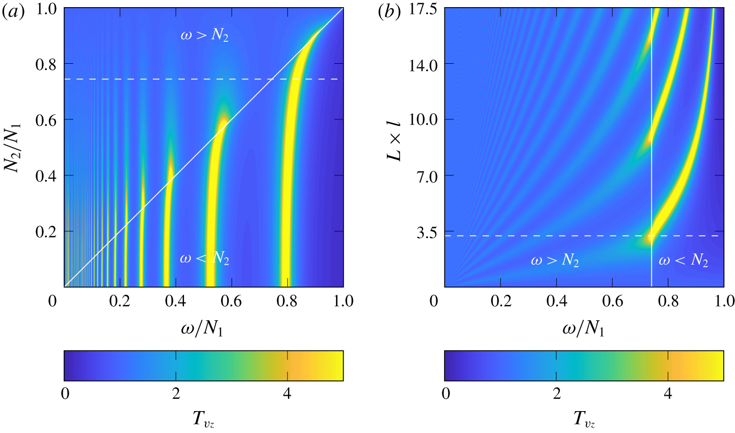
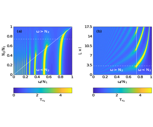
 $N_{2}/N_{1}$. Figure 3 presents colour maps of the transmission coefficient for vertical velocity
 $T_{v_{z}}$, as a function of these different parameters. Clear peaks appear, with large amplitudes due to a constructive interference effect between upwards and downwards propagating waves in the upper layer. Figure 3(a) shows the transmission coefficient as a function of
 $\unicode[STIX]{x1D714}/N_{1}$ and
 $N_{2}/N_{1}$ for a fixed value of
 $L\times l$ (
 $=3.23$). Transmission is generally higher for cases where waves can propagate in both regions (
 $\unicode[STIX]{x1D714}<N_{2}<N_{1}$) and drops off for evanescent frequencies in the lower region (
 $N_{2}<\unicode[STIX]{x1D714}<N_{1}$). Maxima of transmission appear for well-defined values of
 $\unicode[STIX]{x1D714}/N_{1}$ at a given
 $N_{2}/N_{1}$. The curves defining the maxima of transmission are continuous between the evanescent and the propagating regions. Figure 3(b) shows the transmission coefficient as a function of
 $\unicode[STIX]{x1D714}/N_{1}$ and
 $L\times l$ for a fixed value of
 $N_{2}/N_{1}$ (
 $=0.74$). The cutoff between the propagating and evanescent regions is now observed at
 $\unicode[STIX]{x1D714}/N_{1}=N_{1}/N_{2}=0.74$. The resonant interference peaks are expected to be less numerous as
 $N_{2}/N_{1}\rightarrow 1$ or as
 $L\times l\rightarrow 0$. The study of the transmission coefficient in radial velocity
 $T_{v_{r}}$ shows similar behaviour.
Colour maps of the transmission coefficient  $T_{v_{z}}$ as a function of (a)
 $\unicode[STIX]{x1D714}/N_{1}$ and
 $N_{1}/N_{2}$ at a given
 $L\times l=3.23$, and (b)
 $\unicode[STIX]{x1D714}/N_{1}$ and
 $L\times l$ at a given
 $N_{2}/N_{1}=0.74$. Dashed lines show the cuts at (a)
 $N_{2}/N_{1}=0.74$ and (b)
 $L\times l=3.23$. The Coriolis frequency is set to be
 $f=0$.

2.3.2 Smooth interface
As in the freely incoming wave case, these results can be extended to the case of a smooth interface through the same method, simply by changing the boundary condition at the surface,
 $$\begin{eqnarray}\tilde{\unicode[STIX]{x1D719}}(z)=\left\{\begin{array}{@{}ll@{}}\unicode[STIX]{x1D719}_{0},\quad & \text{if}~z=L,\\ \unicode[STIX]{x1D719}_{0}^{T}\text{e}^{\text{i}m_{2}z},\quad & \text{if}~z=z^{-},\end{array}\right.\end{eqnarray}$$
where  $z^{-}$ is a location far from the interface in the lower layer, leading to a new set of boundary conditions for the numerical computation.
2.3.3 Weakly viscous correction
The transmission mechanism involved in the confined configuration is supposed to result from an infinite number of reflections in the upper layer. Such a condition, however, is not truly satisfied in the case of a viscous fluid, as the amplitude of the wave field decreases and vanishes after a finite number of reflections. Once again, the problem is solved numerically after finding the correct boundary conditions, using the first-order development of the vertical wavenumber  $m$ (Boury et al. Reference Boury, Peacock and Odier2019).
3 Experimental apparatus
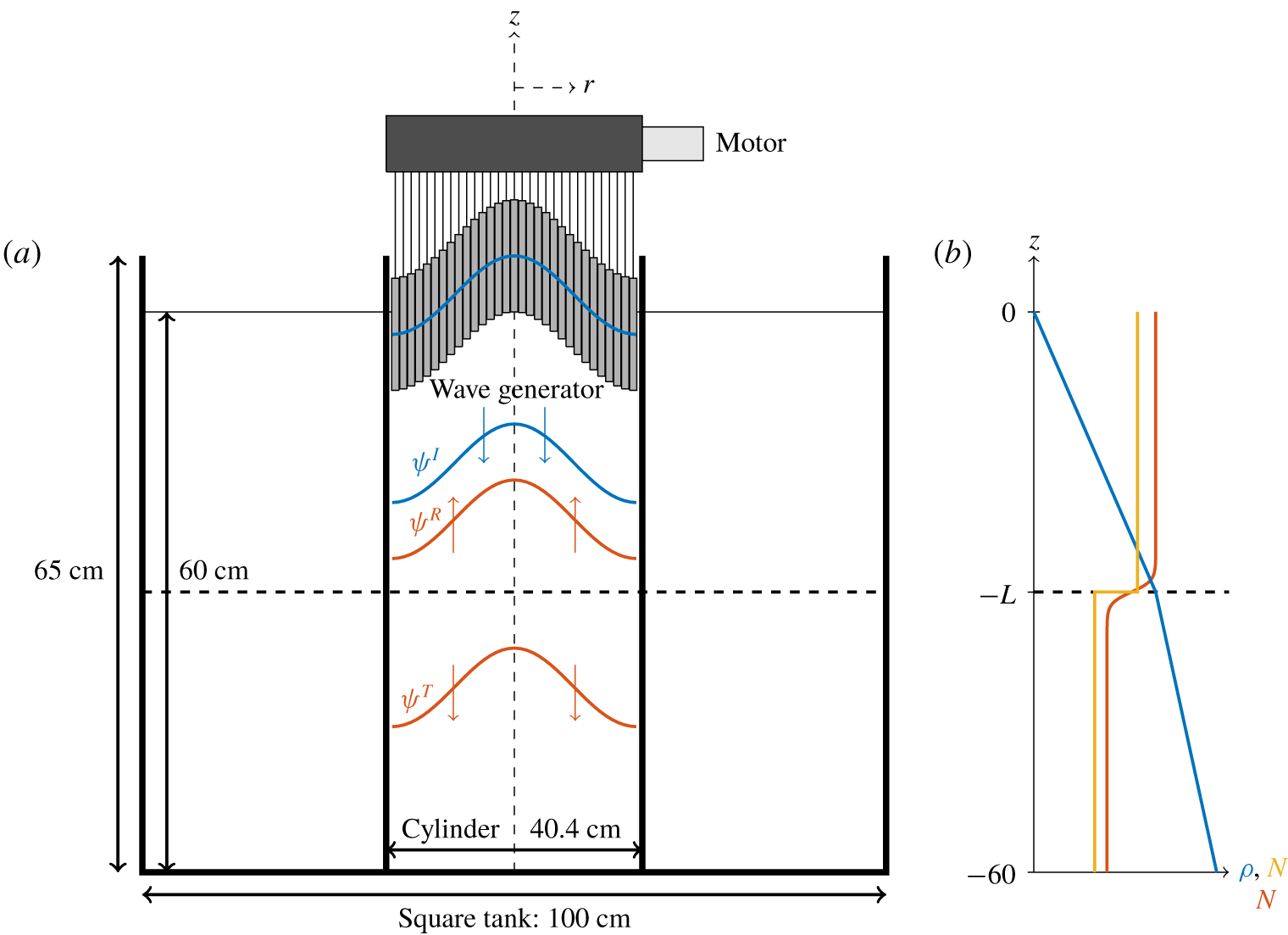
The experimental arrangement described in Boury et al. (Reference Boury, Peacock and Odier2019) is used to investigate the transmission of internal waves across a buoyancy frequency interface. The experiments did not involve rotation ( $f=0$), so the waves were purely internal gravity waves. Note that adding rotation at fixed values of
 $N$,
 $\unicode[STIX]{x1D714}$ and
 $l$, would only change the vertical wavenumber
 $m$ and not the physics involved in the linear theory (see (2.4)). A schematic is presented in figure 4. Experiments were conducted in a cylindrical acrylic tank of diameter 40.4 cm, inserted into a square acrylic tank of
 $100~\text{cm}\times 100~\text{cm}$ horizontal section and 65 cm height. Both were filled with salt-stratified water with the same density profile to avoid optical deformations.
(a) Schematic of the experimental apparatus. (b) Idealised density profile with corresponding sharp and smooth buoyancy frequency profiles.

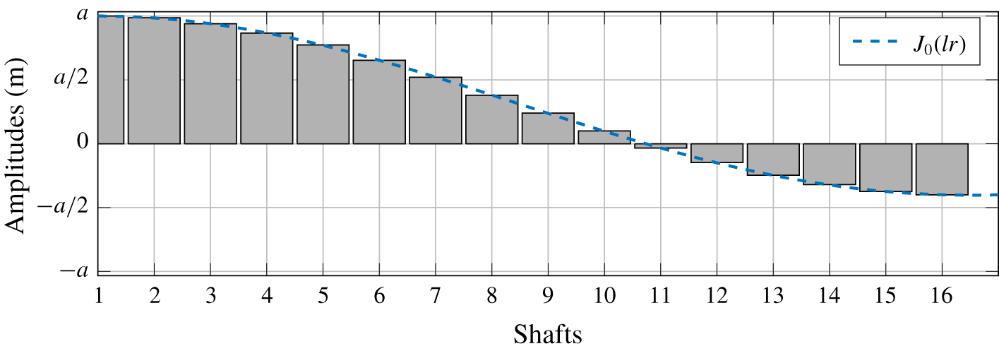
Internal waves are produced using Maurer et al.’s axisymmetric wave generator (Maurer et al. Reference Maurer, Ghaemsaidi, Joubaud, Peacock and Odier2017). This device, adapted from Gostiaux et al.’s planar wave generator (Gostiaux et al. Reference Gostiaux, Didelle, Mercier and Dauxois2006), comprises 16 concentric cylinders moving with customisable eccentricities, enabling us to excite axisymmetric wave patterns. We set its configuration to be a mode 1 profile able to produce pure cylindrical modes shaped as Bessel functions (Boury et al. Reference Boury, Peacock and Odier2019). The profile of the mode 1 configuration, with a radial wavelength of  $l=19~\text{m}^{-1}$, is presented in figure 5. We use a generator amplitude
 $a=2.5~\text{mm}$, which is low enough to limit nonlinear effects (see appendix A).
Configuration of the generator ( $l=19~\text{m}^{-1}$). The amplitude
 $a$ is set to 2.5 mm.

We adapted the double bucket method (Fortuin Reference Fortuin1960; Oster & Yamamoto Reference Oster and Yamamoto1963) to fill the tank with salt-stratified water. In order to obtain bi-linear stratifications, when required we stopped the filling, to change the filling tank density difference by removing salty water and adding fresh water without changing the density in the mixing tank. We then re-started the filling, which gave us a sharp but continuous buoyancy frequency interface at the desired depth. Density and buoyancy frequency profiles were measured using calibrated precision measurement engineering conductivity and temperature probes mounted on a motorised vertical axis. Buoyancy frequencies of each layer are estimated from the mean values of the  $N$ profile, obtained after smoothing the density function
 $\unicode[STIX]{x1D70C}(z)$ and taking its derivative. Errors on the buoyancy frequency are estimated using the standard deviation of this
 $N$ profile and are in most cases approximately 4 % of the estimated
 $N$ value. In our experiments, we decided to use a stronger stratification in the upper layer (
 $N_{1}>N_{2}$), as in the theory, because we wanted to look at transmission when the wave field in the lower layer was either propagating or evanescent.
Experiments were conducted over a period of time up to 40 hours during which the interface becomes less sharp due to diffusive effects (we estimate the width of the interface to increase at a rate of approximately  $1~\text{cm}~\text{day}^{-1}$). Due to the configuration of the apparatus, the stratification could not be measured at different times while running the experiment because the presence of the generator prevented access to the domain of interest by the conductivity probe. As detailed later in the result section, however, we conducted systematic repeated experiments showing that any evolution of the stratification did not impact the experimental results.
Visualisation of the velocity fields was performed using particle image velocimetry (PIV). A vertical laser plane, containing the generator diameter, was created using a 2 W Ti:sapphire laser (at 532 nm) and a cylindrical lens. Hollow glass spheres of  $10~\unicode[STIX]{x03BC}\text{m}$ diameter were added to the salt-stratified fluid for the purpose of visualisation. A camera recorded particle displacements at 1 Hz in the laser plane. The CIVx (correlation imaging velocimetry) algorithm was subsequently used to process the PIV raw images and extract the velocity fields (Fincham & Delerce Reference Fincham and Delerce2000).
4 Results
4.1 Transmission of a free incident wave
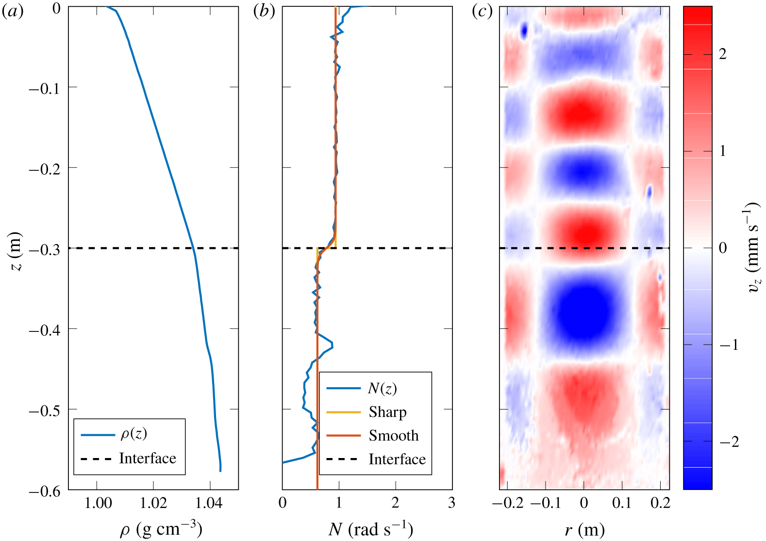
From left to right: (a) density profile  $\unicode[STIX]{x1D70C}(z)$, (b) buoyancy frequency profile
 $N(z)$ and fits (with
 $N_{1}=0.94\pm 0.02~\text{rad}~\text{s}^{-1}$,
 $N_{2}=0.62\pm 0.05~\text{rad}~\text{s}^{-1}$,
 $L=30~\text{cm}$, width
 $\unicode[STIX]{x1D6FF}=1~\text{cm}$) and (c) example of vertical PIV cross-section of the vertical velocity field (
 $\unicode[STIX]{x1D714}/N_{1}\simeq 0.4$). The generator is located at the top (
 $z=0$). The dashed line indicates the interface.

We first quantified the transmission coefficient for the vertical velocity field in the case of a freely incoming wave. To conduct this experiment, a two-layer stratification is used and a range of forcing frequencies are explored. For each frequency, the transmission coefficient is extracted from the PIV data by looking at the vertical velocity below the interface.
Figure 6 presents the stratification used to conduct this study. The first two plots show the density profile  $\unicode[STIX]{x1D70C}(z)$ computed from the measurements of the conductivity/temperature (C/T) probe, and the buoyancy frequency profile
 $N(z)$ subsequently derived. The density curve shows two layers of linear stratification, one from 0 to 30 cm and one from 30 to 60 cm. The buoyancy frequency profile confirms this trend, showing two constant values for the density gradient:
 $N_{1}=0.94\pm 0.02~\text{rad}~\text{s}^{-1}$ and
 $N_{2}=0.62\pm 0.05~\text{rad}~\text{s}^{-1}$. We indicate by a dashed line the interface between these two domains, and by a straight line the top of the tank. Two to three centimetres are missed in the measurements at the bottom of the tank, due to the configuration of the probe. On the buoyancy frequency curve, we fit the
 $N$ profile with our models for a sharp and a smooth interface (2.9) with the same distance
 $L=30~\text{cm}$ from the generator, and a width
 $\unicode[STIX]{x1D6FF}=1~\text{cm}$. No error is given on these lengths because it does not impact the transmission coefficient error, as we will discuss later. A small bump in the stratification is present at 42 cm below the generator: its width on the
 $N$ profile is exaggerated because of the averaging process used to compute the buoyancy frequency and, as can be seen in figure 6(c), it does not affect the velocity field. However, to get the most accurate evaluation of
 $N_{2}$, we used the mean value and the standard deviation in the interval [31; 41] cm. The
 $N_{1}$ profile was estimated in the [3; 28] cm interval.
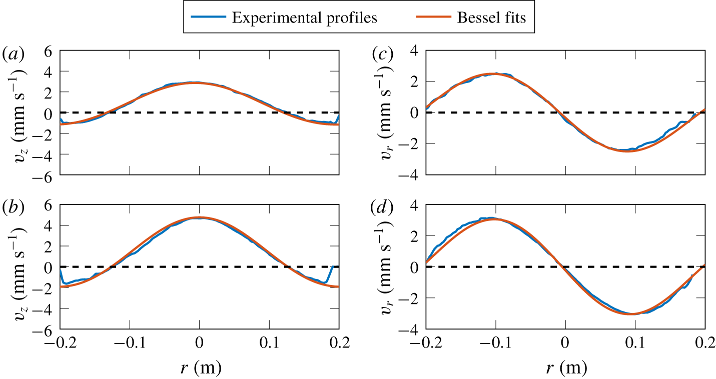
Experimental profiles and fits with Bessel functions: (a) vertical velocity in the upper layer, at  $z\simeq -15~\text{cm}$; (b) vertical velocity in the lower layer, at
 $z\simeq -35~\text{cm}$; (c) radial velocity in the upper layer, at
 $z\simeq -15~\text{cm}$; (d) radial velocity in the lower layer, at
 $z\simeq -35~\text{cm}$. Profiles are taken at random times.

Figure 6(c) presents a PIV snapshot of the vertical velocity field after the wave field crossed the buoyancy frequency interface. The mode $-1$ shape of the generator in a horizontal plane is visible at the top due to a parallax effect. Through the interface, we see that the radial wavelength, given by the horizontal nodes and antinodes of the field, is conserved. The vertical wavenumber, given by the vertical nodes and antinodes (Boury et al. Reference Boury, Peacock and Odier2019), changes when the wave field crosses the interface, and is lower in the bottom layer than in the top one. Such a behaviour is expected, as the vertical wavenumber
 $m$ is fixed by the buoyancy frequency
 $N$ and in our experiment we set
 $N_{2}<N_{1}$.
To ensure that the interface does not affect the modal shape of the field, we present in figure 7 horizontal profiles of the radial and vertical velocity fields in the upper layer and in the lower layer. Without any regard to the amplitude, as the profiles were taken at random times, we see that in both cases the fits with the expected Bessel functions respectively  $J_{0}(lr)$ and
 $J_{1}(lr)$, with
 $l=19~\text{m}^{-1}$, agree well with the experimental profiles.
The transmission properties are investigated using the stratification from figure 6, by producing mode $-1$ wave fields first for increasing frequencies
 $\unicode[STIX]{x1D714}=0.3$ to
 $0.98~\text{rad}~\text{s}^{-1}$ (labelled by
 $\unicode[STIX]{x1D714}_{{\nearrow}}$), then for decreasing frequencies
 $\unicode[STIX]{x1D714}=0.96$ to
 $0.28~\text{rad}~\text{s}^{-1}$ (labelled by
 $\unicode[STIX]{x1D714}_{{\searrow}}$). As no direct measurement of the stratification can be performed inside the cylinder due to the lateral, top and bottom boundaries, this protocol serves as a check that the stratification does not change while running the experiment. Because we only want to investigate the transmission of the wave field, short-time measurements are done with excitations of 100 s, at 20 min intervals each, to ensure that the fluid is initially at rest for each measurement. We measure the amplitude in the lower region, after the wave has crossed the interface. To this extent, the selection procedure described in Boury et al. (Reference Boury, Peacock and Odier2019) is adapted.
We consider the time series obtained by fitting horizontal cuts of vertical velocity for Bessel functions of radial number  $l=19~\text{m}^{-1}$. These cuts are taken at a depth
 $z_{m}$, a few centimetres below the interface. In this time series, we pick three different time windows of one-period width, starting at a time when
 $v_{z}=0$, half-covering each other. The middle time window is chosen to be the last one before the wave reflected at the bottom returns at
 $z=z_{m}$. This returning time,
 $t_{f}$, is determined using the group velocity
 $$\begin{eqnarray}\boldsymbol{v}_{\boldsymbol{g}}=-\frac{ml^{2}N^{2}}{\unicode[STIX]{x1D714}k^{4}}\boldsymbol{e}_{\boldsymbol{z}}\end{eqnarray}$$
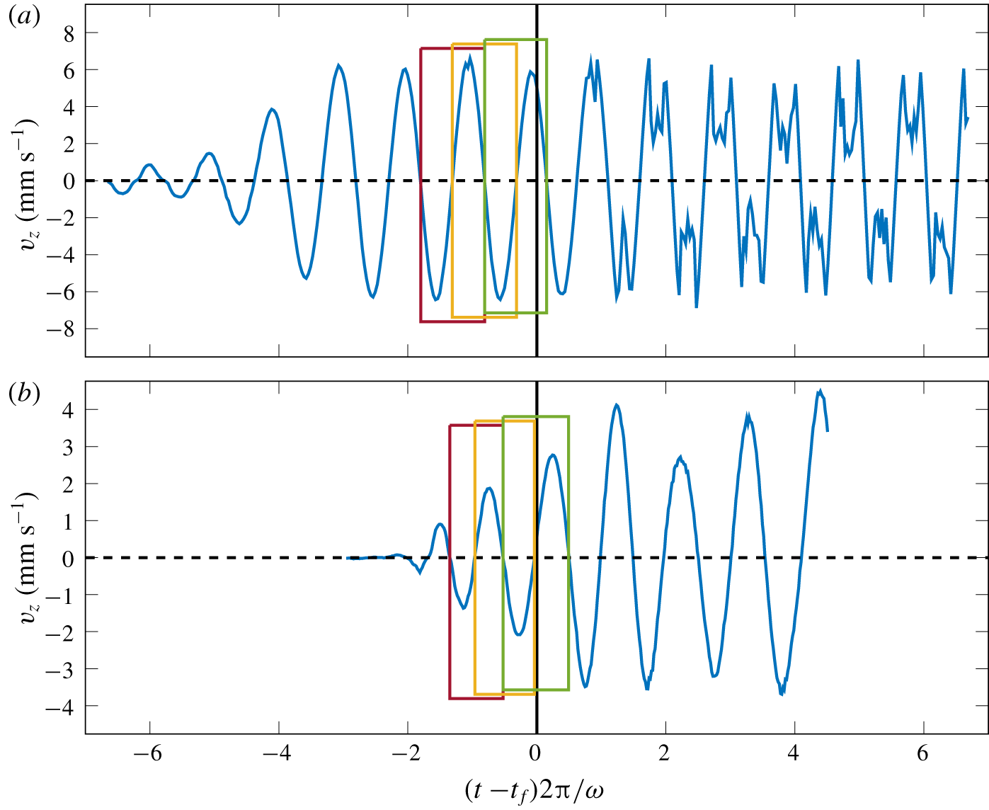
computed in both layers. Figure 8 shows examples of (a) time series at  $\unicode[STIX]{x1D714}/N_{1}=0.89$ and (b) time series at
 $\unicode[STIX]{x1D714}/N_{1}=0.50$, with the three different time windows used to estimate the amplitude in both cases. The wave field in figure 8(a) is evanescent in the lower region, so there is theoretically no reflected wave. In this case, the time
 $t_{f}$ is taken just before seeing nonlinearities. In the measurement region, the temporal evolution of the amplitude is nearly sinusoidal. In figure 8(b), the amplitude is still growing after the returning time. This can be due to the reflected wave, or to a non-fully established wave field.
For each of the three time windows defined, the root-mean-square (r.m.s.) value of the time signal during the chosen time windows is computed. The wave amplitude is then defined as the average of the three values obtained, multiplied by  $\sqrt{2}$ since the signal is fairly sinusoidal. The standard deviation between these three values gives an estimate of the measurement error. The need for such a process is justified by the fact that, for some frequencies, the wave field is not fully developed when reaching the interface (figure 8). Given this situation, measuring the right amplitude is difficult even when the profiles are well fitted by the theoretical Bessel functions.
Time series of the amplitude of the vertical velocity over  $100~\text{s}$, (a) at
 $\unicode[STIX]{x1D714}/N_{1}=0.89$ and (b) at
 $\unicode[STIX]{x1D714}/N_{1}=0.50$. The black solid line indicates the time
 $t_{f}$ used to compute the amplitude. Rectangles show the three periods used to estimate the wave amplitude from the r.m.s.

Direct comparison between the amplitude of the wave field above and under the interface is not possible, because the multiple reflections within the relatively narrow top layer make it infeasible to extract the amplitude of the incident wave alone. However, we have shown in Boury et al. (Reference Boury, Peacock and Odier2019) that, for frequencies above  $\unicode[STIX]{x1D714}/N\simeq 0.3$, the experimental amplitude of an incident mode is well predicted by the generator amplitude
 $a\unicode[STIX]{x1D714}$, corrected with the theoretical viscous damping coefficient
 $$\begin{eqnarray}v_{z,inc}=a\unicode[STIX]{x1D714}\times \exp (-\unicode[STIX]{x1D700}m_{1}^{(1)}L),\end{eqnarray}$$
where  $m_{1}^{(1)}$ is defined in § 2.2.3. Therefore, to estimate the transmission coefficient, we compare the measured transmitted amplitude
 $v_{z,mes}$ to the theoretical incident amplitude
 $v_{z,inc}$:
 $$\begin{eqnarray}T_{v_{z}}=\frac{v_{z,mes}}{v_{z,inc}}=\frac{v_{z,mes}}{a\unicode[STIX]{x1D714}\times \exp (-\unicode[STIX]{x1D700}m_{1}^{(1)}L)}.\end{eqnarray}$$
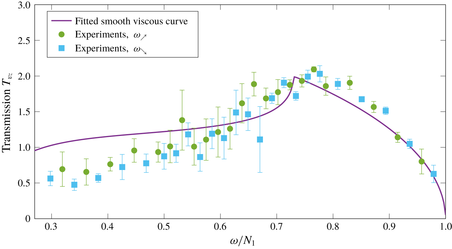
The experimental transmission data points are presented in figure 9. To scale the frequencies as a non-dimensional parameter, we use the mean value of the buoyancy frequency  $N_{1}$. We note that, as the two sets of measurements
 $\unicode[STIX]{x1D714}_{{\nearrow}}$ and
 $\unicode[STIX]{x1D714}_{{\searrow}}$ nicely follow the same trend, the influence of the forcing on the stratification can be considered as negligible. In order to draw comparisons with theoretical predictions, we must first make some considerations on the control parameters. The shape of the theoretical curves is controlled by various parameters: the position of the interface
 $L$, its width
 $\unicode[STIX]{x1D6FF}$ and the buoyancy frequencies of the two layers
 $N_{1}$ and
 $N_{2}$. We studied the impact of these parameters by computing different curves for the smooth interface with a weakly viscous correction using the method explained in §§ 2.2.2 and 2.2.3. We found that the distance
 $L$ mainly controls the viscous damping observed at low frequencies, as the amplitude of the wave is greatly attenuated for
 $\unicode[STIX]{x1D714}/N_{1}<0.5$, as discussed in Boury et al. (Reference Boury, Peacock and Odier2019). The width
 $\unicode[STIX]{x1D6FF}$ changes the height of the peak in the transmission curve, located at
 $\unicode[STIX]{x1D714}/N_{1}=N_{2}/N_{1}$. However, as the interface is really sharp in our experiment (
 $\unicode[STIX]{x1D6FF}=1~\text{cm}$), its impact is negligible. To investigate the influence of the buoyancy frequencies, we looked at the ratio
 $N_{2}/N_{1}$. We found that the transmission curve is very sensitive to a slight change in the buoyancy frequencies, as it shifts the position of the transmission peak and defines the range of frequencies for which the wave is transmitted or fully reflected.
As discussed at the beginning of this section, we measured  $N_{1}=0.94\pm 0.02~\text{rad}~\text{s}^{-1}$ and
 $N_{2}=0.62\pm 0.05~\text{rad}~\text{s}^{-1}$. As a result, we have
 $N_{2}/N_{1}=0.66\pm 0.06$. Due to the fairly large uncertainty on this value, however, we decided to compute numerically the transmission curves for a smooth interface with a weakly viscous correction, leaving the ratio
 $N_{2}/N_{1}$ as a free parameter that we adjust by ensuring that the position of the transmission peak in this curve corresponds to the data. This adjusted curve is shown in figure 9. The resulting fitted value of
 $N_{2}/N_{1}$ is 0.73, which is within the uncertainty of our experimental estimate for this ratio.
We can now discuss how the experimental data points compare with the theory for a smooth interface and weak viscous effects. The general trend is very similar, with an increased transmission as the frequency is increased, until one reaches a maximum of  $T_{v_{z}}=2$ at a frequency close to the buoyancy frequency of the lower layer, as expected since the waves then become evanescent in this region. Then, one observes a sharp decrease of the transmission. Above
 $\unicode[STIX]{x1D714}/N_{1}\simeq 0.5$, which is the region of interest with the maximum of transmission, the experimental data points show good agreement with the theoretical curve. In contrast, in the region
 $0.3<\unicode[STIX]{x1D714}/N_{1}<0.5$, the data points are below the theoretical prediction. We assume that this trend for low values of
 $\unicode[STIX]{x1D714}/N_{1}$ is due to the poor efficiency of the apparatus at these frequencies, because of boundary layer damping effects on the cylinder (Beckebanze et al. Reference Beckebanze, Brouzet, Sibgatullin and Maas2018; Boury et al. Reference Boury, Peacock and Odier2019), which are not taken into account in our weakly viscous model. An order of magnitude of these effects gives, at low frequency, a damping in amplitude of up to a factor 2, relevant to what is observed.
Experimental transmission curve. We fit the experimental data with a theoretical curve computed for a smooth interface with viscosity (straight line).

4.2 Transmission of a confined incident wave
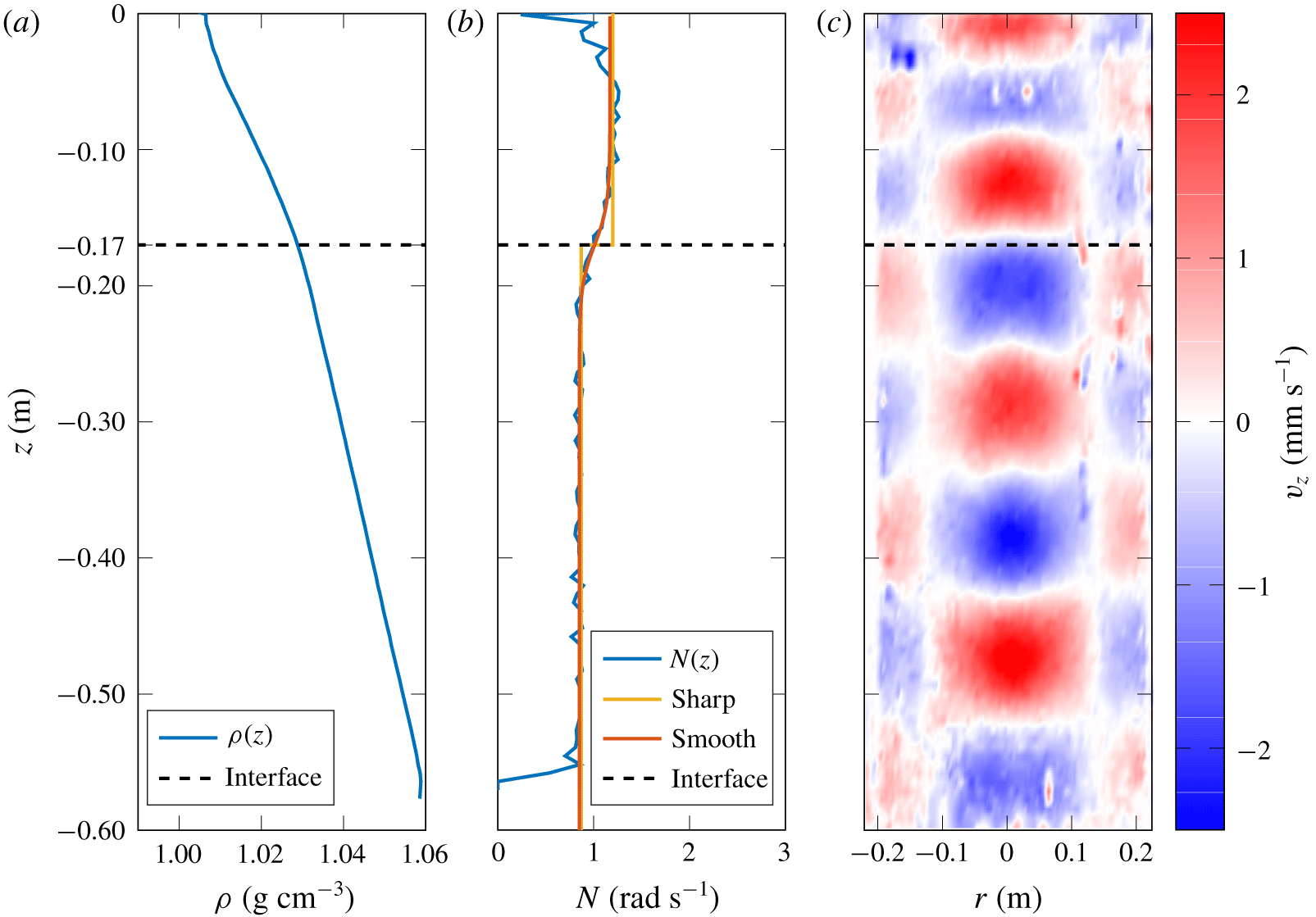
We now focus on the confined wave configuration. Figure 10 shows the experimental stratification used in this study, with (a) the density and (b) the buoyancy frequency profiles, computed as in the previous section. We use a two-layer stratification: the top layer is from 0 to 17 cm, with  $N_{1}=1.17\pm 0.07~\text{rad}~\text{s}^{-1}$, and the bottom layer is from 17 to 60 cm, with
 $N_{2}=0.85\pm 0.03~\text{rad}~\text{s}^{-1}$. A dashed line indicates the location of the interface, and a straight line shows the water surface. The buoyancy frequency profile is fitted with a sharp interface curve and a smooth interface curve, with the same distance
 $L=17~\text{cm}$, and a width
 $\unicode[STIX]{x1D6FF}=3~\text{cm}$ for the smooth interface. We see an important mixed layer at the surface, which is part of the upper layer and we make sure that
 $N_{1}$ is estimated outside this layer. We compute
 $N_{1}$ in the interval [2; 15] cm and
 $N_{2}$ using the interval [22; 53] cm. Figure 10(c) presents an example of a PIV field for the vertical velocity in this experiment. Between the generator, at the surface and the interface, we can see that the wave field has a smaller vertical wavelength than below the interface, consistent with
 $N_{2}<N_{1}$, as in the previous experiment.
From left to right: (a) density profile  $\unicode[STIX]{x1D70C}(z)$, (b) buoyancy frequency profile
 $N(z)$ and fits (with
 $N_{1}=1.17\pm 0.07~\text{rad}~\text{s}^{-1}$,
 $N_{2}=0.85\pm 0.03~\text{rad}~\text{s}^{-1}$,
 $L=17~\text{cm}$, width
 $\unicode[STIX]{x1D6FF}=3~\text{cm}$) and (c) example of vertical PIV cross-section of the vertical velocity field (
 $\unicode[STIX]{x1D714}/N_{1}\simeq 0.36$). The generator is located at the top (
 $z=0$). The dashed line indicates the interface.

Mode $-1$ wave fields for 65 values of frequency from
 $\unicode[STIX]{x1D714}=0.2$ to
 $1.09~\text{rad}~\text{s}^{-1}$ are produced. Given the previous results on transmission in a non-resonant case, we assume that the stratification does not change in our experiment and we only perform the measurements by increasing the frequency. We also use short-time excitations of 100 s at 20 min interval each. Amplitudes are measured below the interface in a similar selection process as before, but the position of the interface closer to the generator allows for several back and forth reflections in the upper layer. Measurements are compared to the theoretical generator amplitude (4.2) to compute the transmission coefficient.
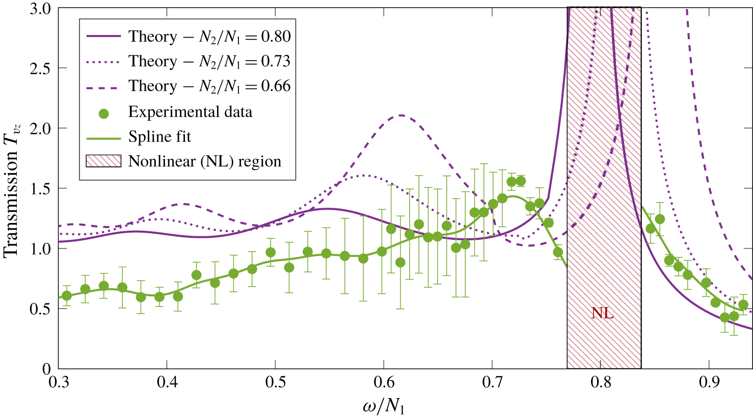
Results are presented in figure 11. Measurements of the transmission coefficient are plotted as a function of  $\unicode[STIX]{x1D714}/N_{1}$, using the mean value of
 $N_{1}$. As in the previous section, we must also investigate the influence of the different parameters
 $L$,
 $\unicode[STIX]{x1D6FF}$,
 $N_{1}$ and
 $N_{2}$, on the theoretical transmission curve for a confined incident wave, a smooth interface and weekly viscous effects obtained following the method described in §§ 2.3.2 and 2.3.3. The length
 $L$ contributes to the peak positions in the propagating region
 $\unicode[STIX]{x1D714}<N_{2}$. The width of the interface
 $\unicode[STIX]{x1D6FF}$ has little impact because the interface is relatively sharp. In contrast, the buoyancy frequencies
 $N_{1}$ and
 $N_{2}$ mainly control the shape of the curve, as they change the position of the peaks, their amplitude as well as the limit between the propagating and evanescent transmissions. Using the C/T probe, we measure
 $N_{1}=1.17\pm 0.07~\text{rad}~\text{s}^{-1}$ and
 $N_{2}=0.85\pm 0.03~\text{rad}~\text{s}^{-1}$, which gives us a ratio
 $N_{2}/N_{1}$ going from 0.8 to 0.66. As a result, several theoretical curves for a smooth interface with viscosity, numerically computed, are presented in figure 11, one for the central value of
 $N_{2}/N_{1}$, namely 0.73, and two others for the extreme values of the ratio, 0.66 and 0.8. It shows that, although the different theoretical curves always present the same trend, with various peaks, the position and height of the peaks can vary a lot by slightly varying the ratio
 $N_{2}/N_{1}$.
Experimental transmission curve for a forced upper layer. Theoretical curves computed for the maximal, mean and minimal values of  $N_{2}/N_{1}$ are plotted. A spline fit (dashed green line) is added to guide the eye on the experimental curve.

Experimental data display the same qualitative behaviour as theoretical predictions. For  $\unicode[STIX]{x1D714}/N_{1}\in [0.17;~0.74]$, the transmission coefficient increases non-monotonically with local extrema. As in the previous section, measurements at low frequencies show a smaller transmission than the expected value, also probably due to boundary layer damping effects (Beckebanze et al. Reference Beckebanze, Brouzet, Sibgatullin and Maas2018; Boury et al. Reference Boury, Peacock and Odier2019). The most significant features, however, occur at higher frequencies and are therefore unaffected by this. For
 $\unicode[STIX]{x1D714}/N_{1}>0.74$ the transmission coefficient is globally decreasing as the waves become evanescent in the lower region. For a given range of frequencies
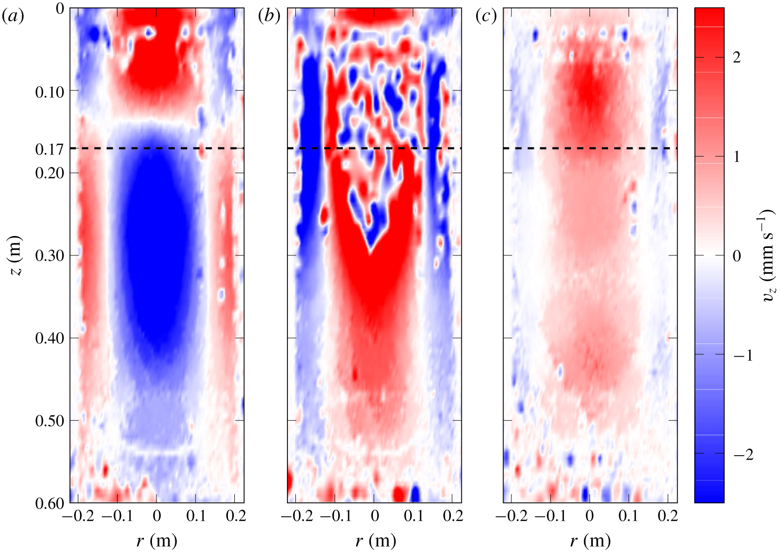
 $\unicode[STIX]{x1D714}/N_{1}\in [0.77;~0.84]$, however, nonlinear effects are triggered and no amplitude can be measured as the wave field is no longer described by our model. This area is indicated by a shaded area in figure 11 and corresponds to the expected resonant interference peak of the theoretical curves. Snapshot examples of the vertical velocity field are given in figure 12 for three different situations after
 $34$ periods of excitation: figure 12(a) shows propagating waves in both layers at
 $\unicode[STIX]{x1D714}/N_{1}=0.7$, while in figures 12(b) and 12(c) waves are evanescent in the lower layer at
 $\unicode[STIX]{x1D714}/N_{1}=0.8$ and
 $\unicode[STIX]{x1D714}/N_{1}=0.9$, respectively. In contrast to the images presented in figures 12(a) and 12(c), the image presented in figure 12(b) shows small-scale disturbances of the wave field resulting from nonlinear effects due to constructive interference in the upper layer, representing the typical behaviour observed within the hatched region identified in figure 11.
Snapshots of the vertical velocity field in three different cases: (a)  $\unicode[STIX]{x1D714}<N_{2}<N_{1}$ and
 $\unicode[STIX]{x1D714}/N_{1}=0.7$; (b)
 $N_{2}<\unicode[STIX]{x1D714}<N_{1}$ and
 $\unicode[STIX]{x1D714}/N_{1}=0.7$; and (c)
 $N_{2}<\unicode[STIX]{x1D714}<N_{1}$ and
 $\unicode[STIX]{x1D714}/N_{1}=0.8$. All pictures are taken at 34 periods of excitation.

5 Application to the ocean: an example
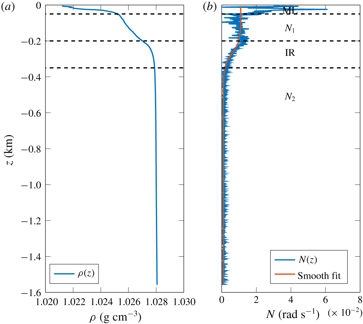
An interesting application of our confined layer studies is to relate our findings to a scenario that has a strong upper ocean stratification overlying a weaker deep ocean stratification. Figure 13 presents an example of density and buoyancy frequency profiles taken at  $159^{\circ }57.111^{\prime }~\text{W}$,
 $73^{\circ }32.439^{\prime }~\text{N}$ during the Stratified Ocean Dynamics of the Arctic research cruise, on the R/V Sikuliaq, in September 2018. A very simple model can be used to describe this stratification at first order: a melting layer (ML) at the surface issued from ice melting with a strong density gradient, and a bi-linear stratification with two buoyancy frequencies
 $N_{1}$ and
 $N_{2}$ below. Using (2.9), such a profile can be fitted with
 $N_{1}\simeq 0.011~\text{rad}~\text{s}^{-1}$ in the upper layer,
 $N_{2}\simeq 0.001~\text{rad}~\text{s}^{-1}$ in the lower layer,
 $L\simeq 250~\text{m}$ from the ML to the centre of the interface region (IR) which has a width
 $\unicode[STIX]{x1D6FF}\simeq 150~\text{m}$. Note that such parameters cannot be obtained in our experiments, due to the dimensions of the apparatus and to the range of buoyancy frequencies we are able to produce (here,
 $N_{1}$ and
 $N_{2}$ are of the same order of magnitude), but the physics involved remains the same.
Example of (a) density profile and (b) buoyancy profile, from in situ measurements. Different layers can be identified between dashed lines, from top to bottom: ML,  $N_{1}$ linear layer (
 $N_{1}$), IR and
 $N_{2}$ linear layer (
 $N_{2}$).

As shown by our study, constructive interference effects may appear and produce a high transmission coefficient value for confined internal waves. These effects, however, arise only when the vertical wavelength  $2\unicode[STIX]{x03C0}/m_{1}$ is larger than the interface width (Mathur & Peacock Reference Mathur and Peacock2009). On the contrary, the interface acts as a smooth density change for the wave and internal waves pass through relatively unaffected. Re-writing equation (2.4) in terms of the radial wavelength
 $2\unicode[STIX]{x03C0}/l$ as
 $$\begin{eqnarray}\frac{2\unicode[STIX]{x03C0}}{m_{1}}=\frac{2\unicode[STIX]{x03C0}}{l}\left(\frac{\unicode[STIX]{x1D714}^{2}-f^{2}}{N_{1}^{2}-\unicode[STIX]{x1D714}^{2}}\right)^{1/2},\end{eqnarray}$$
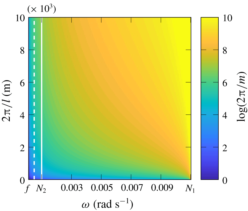
we explore the range of parameters  $(\unicode[STIX]{x1D714};~2\unicode[STIX]{x03C0}/l)$ by plotting the quantity
 $\log (2\unicode[STIX]{x03C0}/m_{1})$ for propagating waves in the upper layer, which means
 $f<\unicode[STIX]{x1D714}<N_{1}$, in figure 14. The Coriolis frequency is set to be
 $f=1.24\times 10^{-4}~\text{rad}~\text{s}^{-1}$, a typical value in this region (Cole et al. Reference Cole, Timmermans, Toole, Krishfield and Thwaites2013).
Logarithmic colour map of the vertical wavelength in the upper layer ( $N_{1}=0.011~\text{rad}~\text{s}^{-1}$) as a function of the frequency
 $\unicode[STIX]{x1D714}$ (from
 $f$ to
 $N_{1}$) and the radial wavelength
 $2\unicode[STIX]{x03C0}/l$. The white solid line represents
 $\unicode[STIX]{x1D714}=N_{2}$, and the white dashed line represents
 $\unicode[STIX]{x1D714}=N_{2}/2$.

Near-inertial wave generation, with frequencies close to  $f$, is found to be easily excited in the Arctic Ocean (Cole et al. Reference Cole, Timmermans, Toole, Krishfield and Thwaites2013), with a small vertical wavelength, as illustrated in figure 14. In this configuration, the factor
 $\unicode[STIX]{x1D714}^{2}-f^{2}$ is of the order of
 $f^{2}$ (
 $10^{-8}~\text{rad}^{2}~\text{s}^{-2}$). Since
 $N_{1}\gg \unicode[STIX]{x1D714}$, the factor
 $N_{1}^{2}-\unicode[STIX]{x1D714}^{2}$ is of the order of
 $N_{1}^{2}$ (
 $10^{-4}~\text{rad}^{2}~\text{s}^{-2}$), yielding
 $l/m_{1}\simeq 10^{-2}$. Hence, to obtain vertical wavelengths of the order of 100 m, the radial wavelength has to be of the order of 10 km, which can be produced by storms of large extent. Higher frequency waves can also be produced (Bell Reference Bell1978; Chini & Leibovich Reference Chini and Leibovich2005; Polton et al. Reference Polton, Smith, MacKinnon and Tejada-Martínez2008), with a frequency of the same order of magnitude as the buoyancy frequency
 $N_{2}$. Hence, the term
 $\unicode[STIX]{x1D714}^{2}-f^{2}$ is of the order of
 $N_{2}^{2}$ (
 $10^{-6}~\text{rad}^{2}~\text{s}^{-2}$), yielding
 $l/m_{1}\simeq 10^{-1}$. As a result, resonant interference waves with vertical wavelength of the order of 100 m can have small radial wavelength (of the order of 1 km).
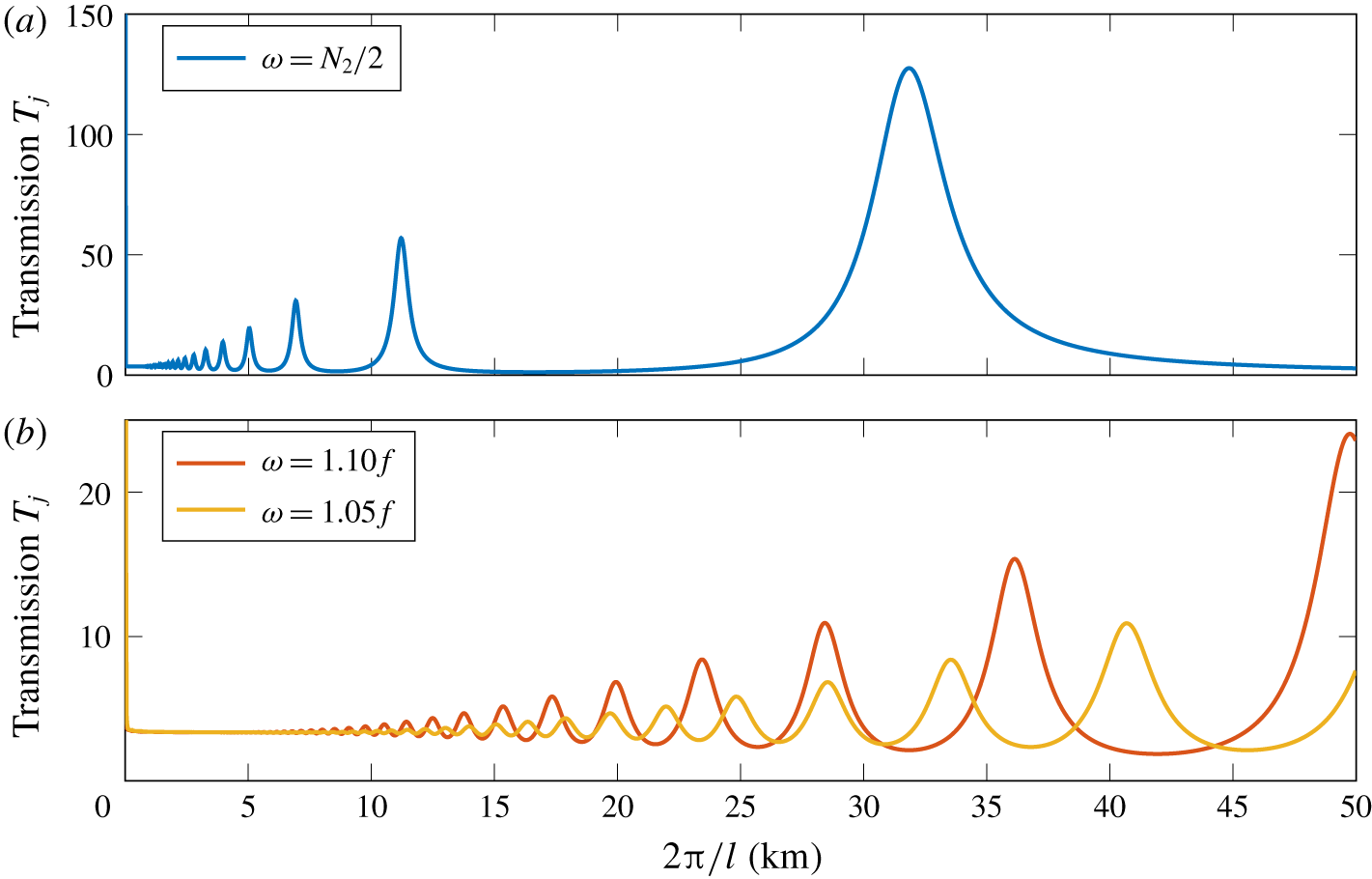
Following the approach of Ghaemsaidi et al. (Reference Ghaemsaidi, Dosser, Rainville and Peacock2016), we present in figure 15 numerical computation of the transmission coefficient for the Arctic stratification (figure 13) for three different frequencies, two of them being near inertial at  $\unicode[STIX]{x1D714}=1.05f$ and
 $\unicode[STIX]{x1D714}=1.1f$, and the third one corresponding to a higher frequency with
 $\unicode[STIX]{x1D714}=N_{2}/2$. A resonant cavity effect, in the sense of constructive interference with sequential peaks of high transmission rate of internal waves, occurs for
 $\unicode[STIX]{x1D714}=N_{2}/2$, for both small and large radial wavelengths. For near-inertial waves, however, the transmission coefficient is almost constant until the vertical wavelength is larger than 10 km, meaning that this enhancement is only relevant for large wavelength storms. In both scenarios the enhancement can be several times, even over an order of magnitude.
Numerical computation of the transmission coefficient as a function of the radial wavelength, for three different frequencies  $1.05f$,
 $1.1f$ and
 $N_{2}/2$, after normalisation by the incoming energy at the surface.

6 Conclusions and discussion
We have presented an experimental study of the propagation of axisymmetric internal wave modes across a buoyancy interface in stratified non-rotating flows. To support our laboratory experiments, we develop a theoretical framework for freely incoming waves and for confined waves, as they represent qualitatively two different scenarios that have relevance to the atmosphere and ocean, respectively.
In this study we find that, despite the additional geometric complexity, with associated features such as an inhomogeneous spatial distribution of energy flux, results for plane waves can be generalised to axisymmetric wave fields. For a free incident wave, we show that the maximum of transmission occurs when the frequency of the wave is equal to the buoyancy frequency of the lower layer. For a confined incident wave, we identify the existence of a constructive interference effect in the upper layer, leading to larger transmission coefficients and potentially nonlinear effects. For both scenarios, theory and experiments show excellent qualitative, and good quantitative, agreement, especially within the range of frequencies containing the resonant interference peaks and the enhanced transmission.
This kind of study can help to shed light on in situ measurements of internal waves signals, for example near-inertial waves in strongly stratified regions such as the Arctic Ocean. Different scenarios can be investigated, such as high frequency internal waves generated by storms at the ocean surface and travelling downwards, or near-inertial waves produced by tides and topography in the deep ocean and travelling upwards. In particular, this latter type of wave can therefore be enhanced through transmission processes and lead to strong signals, although the generation process might be of very low amplitude.
Via a similar mechanism that small-extent staircase stratifications can create selective transmission of internal waves (Ghaemsaidi et al. Reference Ghaemsaidi, Dosser, Rainville and Peacock2016), we show that surface forced nonlinear stratifications can potentially give rise to enhanced transmission to the deep ocean, due to resonant interference effect of internal waves. Nevertheless, for small scale waves of wavelength below 10 km, these effects seem to be limited to high frequencies, while no effect is observed for near-inertial waves. For the latter type of waves, enhanced transmission can however also be observed in the case of very large size disturbances of wavelength above 20 km. We notice that the process involves higher amplification factors as frequency increases, while becoming more selective in terms of wavelength.
These studies could be extended to more complex cases with various layers of different buoyancy frequency, as long as the thickness of the interfaces remains small compared to the vertical wavelength (Nault & Sutherland Reference Nault and Sutherland2007; Ghaemsaidi et al. Reference Ghaemsaidi, Dosser, Rainville and Peacock2016). For a given wave, generated by a storm and observed near the ocean surface, it could help predict the amount of energy that will be carried down towards the deep ocean, as well as the ranges of wavelengths more likely to be transmitted. Such a selection process would lead to a change in the wave features as it travels downwards. Enhanced amplitudes generated by such constructive interference behaviours can also trigger nonlinear effects (Boury et al. Reference Boury, Peacock and Odier2019) producing smaller-scale waves. The mechanisms involved are still to be explained for axisymmetric geometry, and could lead to mixing events, changing the stratification, with subsequent feedback effects on the wave propagation.
Acknowledgements
This work has been partially supported by the ANR through grant ANR-17-CE30-0003 (DisET), ONR Physical Oceanography Grant N000141612450 and by the MIT-France programme. S.B. wants to thank Labex iMust for supporting his research. T.P. thanks ENS de Lyon for travel support funding. The authors also thank R. Supekar for helpful discussions and inputs. This work has been achieved thanks to the resources of PSMN from ENS de Lyon.
Declaration of interests
The authors report no conflict of interest.
Appendix A. A criterion for linearity versus nonlinearity
In this appendix, we use a scale analysis to derive a qualitative criterion allowing us to determine whether the forcing amplitude is low enough to delay the growth of nonlinearities.
In the previous sections, all nonlinear terms in the internal wave equation were neglected and the study only focused on the linear equation. The complete equation, including both linear and nonlinear terms, can be obtained starting from the following set of equations:
 $$\begin{eqnarray}\displaystyle & \displaystyle \unicode[STIX]{x2202}_{t}\unicode[STIX]{x1D6E5}_{h}\unicode[STIX]{x1D713}+{\mathcal{J}}^{\odot }\left(r\unicode[STIX]{x1D713},\frac{\unicode[STIX]{x1D6E5}_{h}\unicode[STIX]{x1D713}}{r}\right)=-\left(\frac{2v_{\unicode[STIX]{x1D703}}}{r}+f\right)\unicode[STIX]{x2202}_{z}v_{\unicode[STIX]{x1D703}}+\unicode[STIX]{x2202}_{r}b, & \displaystyle\end{eqnarray}$$
 $$\begin{eqnarray}\displaystyle & \displaystyle \unicode[STIX]{x2202}_{t}v_{\unicode[STIX]{x1D703}}+\frac{1}{r^{2}}{\mathcal{J}}^{\odot }(r\unicode[STIX]{x1D713},rv_{\unicode[STIX]{x1D703}})=f\unicode[STIX]{x2202}_{z}\unicode[STIX]{x1D713}, & \displaystyle\end{eqnarray}$$
 $$\begin{eqnarray}\displaystyle & \displaystyle \unicode[STIX]{x2202}_{t}b+\frac{1}{r}{\mathcal{J}}^{\odot }(r\unicode[STIX]{x1D713},b)=-N^{2}\frac{1}{r}\unicode[STIX]{x2202}_{r}(r\unicode[STIX]{x1D713}), & \displaystyle\end{eqnarray}$$
coupling the axisymmetric streamfunction  $\unicode[STIX]{x1D713}$ to the azimuthal velocity
 $v_{\unicode[STIX]{x1D703}}$ and the buoyancy field
 $b$. The Laplacian
 $\unicode[STIX]{x1D6E5}_{h}\unicode[STIX]{x1D713}$ is defined by
 $$\begin{eqnarray}\unicode[STIX]{x1D6E5}_{h}\unicode[STIX]{x1D713}={\displaystyle \frac{\unicode[STIX]{x2202}^{2}\unicode[STIX]{x1D713}}{\unicode[STIX]{x2202}z^{2}}}+{\displaystyle \frac{\unicode[STIX]{x2202}}{\unicode[STIX]{x2202}r}}\left(\frac{1}{r}{\displaystyle \frac{\unicode[STIX]{x2202}(r\unicode[STIX]{x1D713})}{\unicode[STIX]{x2202}r}}\right)={\displaystyle \frac{\unicode[STIX]{x2202}^{2}\unicode[STIX]{x1D713}}{\unicode[STIX]{x2202}z^{2}}}+{\displaystyle \frac{\unicode[STIX]{x2202}^{2}\unicode[STIX]{x1D713}}{\unicode[STIX]{x2202}r^{2}}}+\frac{1}{r}{\displaystyle \frac{\unicode[STIX]{x2202}\unicode[STIX]{x1D713}}{\unicode[STIX]{x2202}r}}-\frac{\unicode[STIX]{x1D713}}{r^{2}},\end{eqnarray}$$
and the cylindrical Jacobian  ${\mathcal{J}}^{\odot }$ of two functions
 $f$ and
 $g$ is given by
 $$\begin{eqnarray}{\mathcal{J}}^{\odot }(f,g)={\displaystyle \frac{\unicode[STIX]{x2202}f}{\unicode[STIX]{x2202}r}}{\displaystyle \frac{\unicode[STIX]{x2202}g}{\unicode[STIX]{x2202}z}}-{\displaystyle \frac{\unicode[STIX]{x2202}g}{\unicode[STIX]{x2202}r}}{\displaystyle \frac{\unicode[STIX]{x2202}f}{\unicode[STIX]{x2202}z}}.\end{eqnarray}$$
After some calculus, these equations collapse into
 $$\begin{eqnarray}\unicode[STIX]{x2202}_{t}^{2}\unicode[STIX]{x1D6E5}_{h}\unicode[STIX]{x1D713}+N^{2}\unicode[STIX]{x2202}_{r}\left(\frac{1}{r}\unicode[STIX]{x2202}_{r}(r\unicode[STIX]{x1D713})\right)+f^{2}\unicode[STIX]{x2202}_{z}^{2}\unicode[STIX]{x1D713}={\mathcal{N}}{\mathcal{L}},\end{eqnarray}$$
where  ${\mathcal{N}}{\mathcal{L}}$ denotes the nonlinear terms
 $$\begin{eqnarray}{\mathcal{N}}{\mathcal{L}}=-\unicode[STIX]{x2202}_{t}{\mathcal{J}}^{\odot }\left(r\unicode[STIX]{x1D713},\frac{\unicode[STIX]{x1D6E5}_{h}\unicode[STIX]{x1D713}}{r}\right)-f\unicode[STIX]{x2202}_{z}\frac{1}{r^{2}}{\mathcal{J}}^{\odot }(r\unicode[STIX]{x1D713},rv_{\unicode[STIX]{x1D703}})-\unicode[STIX]{x2202}_{r}\left(\frac{1}{r}{\mathcal{J}}^{\odot }(r\unicode[STIX]{x1D713},b)\right)-\frac{1}{r}\unicode[STIX]{x2202}_{t}\unicode[STIX]{x2202}_{z}v_{\unicode[STIX]{x1D703}}^{2}.\end{eqnarray}$$
Let us now consider a scale analysis. The streamfunction amplitude  $\unicode[STIX]{x1D713}_{0}$ is a relevant scaling to be considered. As all frequencies are of the same order of magnitude,
 $\unicode[STIX]{x1D714}$,
 $N$ and
 $f$, are assumed to have the same scaling in
 $1/T$ with
 $T$ the period of the forcing. Disregarding boundary layer effects, the
 $r$ and
 $z$ derivatives are also assumed to have the same scaling in
 $1/L$, with
 $L$ a given length scale. Under these assumptions, the linear part of the equation scales as
 $$\begin{eqnarray}\frac{\unicode[STIX]{x1D713}_{0}}{T^{2}L^{2}}\end{eqnarray}$$
and all nonlinear terms scale as
 $$\begin{eqnarray}\frac{\unicode[STIX]{x1D713}_{0}^{2}}{TL^{4}}.\end{eqnarray}$$
Nonlinear terms have to be taken into account as soon as both scalings are of the same order of magnitude, but they can be neglected if
 $$\begin{eqnarray}\frac{\unicode[STIX]{x1D713}_{0}}{T^{2}L^{2}}\gg \frac{\unicode[STIX]{x1D713}_{0}^{2}}{TL^{4}},\end{eqnarray}$$
which means
 $$\begin{eqnarray}\frac{L^{2}}{\unicode[STIX]{x1D713}_{0}T}\gg 1.\end{eqnarray}$$
The length scale  $L$ can be set so that
 $L\sim 1/l$,
 $l$ being the radial wavenumber. Given that
 $\unicode[STIX]{x1D713}_{0}$ is the amplitude of the streamfunction, the amplitude of the vertical velocity is
 $\unicode[STIX]{x1D713}_{0}l$ with
 $l$ the radial wavenumber and the amplitude of the vertical displacement is
 $\unicode[STIX]{x1D713}_{0}l/\unicode[STIX]{x1D714}\sim \unicode[STIX]{x1D713}_{0}lT$. Setting
 $a$ to be the amplitude of the wave generator, a criterion stating that nonlinear effects are small is
 $$\begin{eqnarray}a\ll 1/l.\end{eqnarray}$$
In this experiment,  $l=19~\text{m}^{-1}$ and
 $1/l=5~\text{cm}$. The generator amplitude should be one order of magnitude lower to prevent nonlinear effects appearing too early, which means a few millimetres. As we have
 $a=2.5~\text{mm}$, this condition is satisfied.