Individual evolutionary learning with many agents

Jasmina Arifovic; John Ledyard

doi:10.1017/S026988891200015X

Individual evolutionary learning with many agents

Published online by Cambridge University Press: 26 April 2012

Jasmina Arifovic and

John Ledyard

Show author details

Jasmina Arifovic*: Affiliation:
Department of Economics, Simon Fraser University, 8888 University Drive, Burnaby, BC V5A 1S6, Canada; e-mail: arifovic@sfu.ca
John Ledyard*: Affiliation:
Division of Humanities and Social Sciences, California Institute of Technology, 1200 East California Boulevard, MC 228-77, Pasadena, CA 91125, USA; e-mail: jledyard@hss.caltech.edu

Article contents

Abstract
Introduction
Description of the learning algorithm
Procedures and results
Final remarks
Footnotes
References

Rights & Permissions

Abstract

Individual Evolutionary Learning (IEL) is a learning model based on the evolution of a population of strategies of an individual agent. In prior work, IEL has been shown to be consistent with the behavior of human subjects in games with a small number of agents. In this paper, we examine the performance of IEL in games with many agents. We find IEL to be robust to this type of scaling. With the appropriate linear adjustment of the mechanism parameter, the convergence behavior of IEL in games induced by Groves–Ledyard mechanisms in quadratic environments is independent of the number of participants.

Information

Type: Articles
Information: The Knowledge Engineering Review , Volume 27 , Special Issue 2: Agent-Based Computational Economics , 26 April 2012 , pp. 239 - 254

DOI: https://doi.org/10.1017/S026988891200015X [Opens in a new window]
Copyright: Copyright © Cambridge University Press 2012

1 Introduction

In Arifovic and Ledyard (Reference Arifovic and Ledyard2011), we study Individual Evolutionary Learning (IEL), a behavioral learning model that is applicable to repeated games with large strategy spaces, including the continuum. In that paper, we used IEL in the games generated by Groves–Ledyard (GL) mechanisms in a quadratic environment. The GL mechanism solves the free-rider problem for public goods. Agents send messages that determine the size of the public good. Agents are taxed, based on the messages they send and on the difference between their message and the average of the other agents’ messages. The mechanism is balanced and efficient. That is, the mechanism collects exactly the taxes needed to pay for the amount of the public good produced and, at the Nash Equilibrium messages, the allocation implied by the public good choice and the taxes is Pareto-optimal. One distinctive feature of the GL mechanisms is a punishment parameter, γ. As this parameter is increased, it creates stronger incentives for each agent to match the average message of the other agents. The particular value of γ does not affect the static properties of the mechanism. It is balanced and efficient for all positive values of γ.

However, dynamic properties, such as the time to converge to Nash Equilibrium in repeated play, do depend on the particular value. Time to converge is very important if these mechanisms are to be used in practice. The welfare (utility or payoff) of the agents is higher the closer to Pareto-optimal allocations they are. Since Nash Equilibria are Pareto-optimal, the faster the agents converge to Nash Equilibrium, the better off they will be over time. Standard theories of dynamics, based on best-reply dynamics and strategic complementarities, suggest that, for these games, there is a number such that if γ is larger than that number then convergence occurs and if γ is smaller then convergence will not occur. Contrary to these standard theories, the prediction from the IEL behavioral model is that the average time to convergence varies smoothly and is U-shaped in γ. We validated these predictions with data from economic experiments with human subjects. However, all of the modeling and experiments were done with five players. Real economies involve many more than that.

In this paper we investigate what happens when the number of players increases. One can imagine many possible conjectures about the effect of numbers on the learning behavior of agents operating in a repeated game context. For example, it is possible that with boundedly rational agents who make mistakes, as occurs in IEL, an increase in numbers could lead to more errors and more erratic behavior by compounding the errors. Alternatively, an increase in numbers could, through the law of large numbers, reduce the variability seen by any one agent, which would enable them to be closer to fully rational behavior.

In this paper we show that if the increase in agents occurs through replication and if the mechanism parameter is normalized for the population size, then the convergence properties of IEL do not depend on the size of the population. That is, let γ be the mechanism parameter, N be the number of agents, and $--><$>T_{c}^{\gamma } <$><$>T_{c}^{\gamma } = f(\gamma /N) <$><!--$ , so that if strategies converge to stage game equilibria in 10 rounds when N = 5 and γ = 50, then strategies will converge in 10 rounds when N = 100 and γ = 1000. Interestingly, the size of the economy does not seem to affect the rate of behavioral learning by IEL.

1.1 Environments, mechanisms, and games

Public-good environments. There are N agents, i∈{1, …, N}. Let z = (X, y ¹, …, y ^N), where X is the amount of the public good and y ⁱ is i's net consumption of the private good. Each agent i begins with an initial endowment of the private good α ⁱ. Agent i's consumption of the private good is α ⁱ + y ⁱ. The per-person cost of production for one unit of the public good is c. The set of feasible allocations is

$--><$$>Z = \left\{ {z = (X,y)|X\,\geqslant{\brvbar}\,0,NcX\, + \,\mathop{\sum}\limits_{i = 1}^N {{{y}^i} } = 0} \right\}\eqno<$$><!--$

Each consumer i has a utility function: $--><$> {{V}^i} (X,{{\alpha }^i} \, + \,{{y}^i} ) = {{A}^i} X\,{\rm{ - }}\,{{B}^i} {{X}^2} \, + \,{{\alpha }^i} \, + \,{{y}^i} <$><!--$ .

We use the notation (N, Z, V) to denote an environment. One allocation of interest in an environment is the one that maximizes the sum of the utilities subject to feasibility. It is easy to see that the X that does this is

$--><$$>\hat{X} = \frac{{\left( {\mathop{\sum}\limits_i {{{A}^i} } } \right)\,{\rm{ - }}\,Nc}}{{2\mathop{\sum}\limits_i {{{B}^i} } }}\eqno<$$><!--$

Groves–Ledyard MechanismsFootnote 2. Begin with a language, a space of messages, M = (−∞, +∞) and m ⁱ∈M can be thought of as i's incremental demand for the public good.

Given a vector of messages m = (m ¹, …, m ^N), the public good produced is

$--><$$>X(m) = \mathop{\sum}\limits_{i = 1}^N {{m}^{_{i} }} \eqno<$$><!--$

The tax to be paid by i is

$--><$$>{{T}^i} (m,\gamma ) = X(m)(c/N)\, + \,(\gamma /2)\left[ {\frac{{N\,{\rm{ - }}\,1}}{N}{{{\left( {{{m}^i} \,{\rm{ - }}\,{{\mu }_{{\rm{ - }}i}}} \right)}}^2} \,{\rm{ - }}\,\sigma _{{{\rm{ - }}i}}^{2} } \right]\eqno<$$><!--$

where γ is an arbitrary free parameter greater than 0, $--><$> {{\mu }_{{\rm{ - }}i}} = {{\mathop{\sum}\nolimits_{h \ne i} {{m}^{_{h} }} } \mathord{\left/ {\vphantom { {(N\,{\rm{ - }}\,1)}}} \right. \kern-\nulldelimiterspace} {(N\,{\rm{ - }}\,1)}} <$><$> \sigma _{{{\rm{ - }}i}}^{2} = \frac{{\mathop{\sum}\nolimits_{h \ne i} {{{({{m}^{_{h} }} \,{\rm{ - }}\,{{\mu }_{{\rm{ - }}i}})}}^2} }}{{N\,{\rm{ - }}\,2}} <$><$> g(m,\gamma ) = (X(m),{{y}^1} (m,\gamma ),\, \ldots, \,{{y}^N} (m,\gamma ))\, =<$><$>(X(m),{\rm{ - }}\,{{T}^1} (m,\gamma ),…,\,{\rm{ - }}{{T}^N} (m,\gamma )) <$><!--$ .

Different values of γ imply different outcome functions and, therefore, different mechanisms. So by letting γ range over values in (0, ∞), one creates an entire class of mechanisms.

Games. An environment and a mechanism combine to create a game, G = {N, H, u}, where N is the number of players, a strategy of i is h ⁱ∈H ⁱ the strategy set of player i, and u ⁱ(h) is the payoff to i if players use h. For the GL mechanism, (M, g(m,γ)), in the public-good environment, (N, Z, V), combining is straightforward. The N players in the game are the N agents in the environment. The strategy set of player i, H ⁱ = M ⁱ. Let $--><$> {{r}^i} (m) = ({{\mu }_{{\rm{ - }}i}}(m),\sigma _{{{\rm{ - }}i}}^{2} (m)) <$><$> {{u}^i} (m) = {{W}^i} ({{m}^i} |{{r}^i} (m),\gamma ) <$><$> X(m) = {{m}^i} \, + \,(N\,{\rm{ - }}\,1){{\mu }_{{\rm{ - }}i}}, <$><!--$

(1)

$--><$$>{{W}^i} ({{m}^i} |{{r}^i} (m),\gamma ) = {{V}^i} ({{m}^i} \, + \,(N\,{\rm{ - }}\,1)r_{1}^{i} (m),{{\alpha }^i} \,{\rm{ - }}\,{{T}^i} ({{m}^i}, {{r}^i} (m),\gamma ))\eqno<$$><!--$

We let G(γ) be the game derived this way. As γ ranges over (0, ∞), a continuum of games is generated. The Nash equilibrium strategy for i in the game G(γ) is h ⁱ(γ) where

(2)

$--><$$>{{\hat{h}}^i} (\gamma ) = \frac{{\hat{X}}}{N}\, + \,\frac{{{{A}^i} \,{\rm{ - }}\,2{{B}^i} \hat{X}\,{\rm{ - }}\,c}}{\gamma }\eqno<$$><!--$

Growing the economy. In this paper we are concerned with what happens as we increase the size of the economy. To keep things comparable as N grows, we consider economies in which larger economies contain replicates of the smaller economies. Let E = (N, Z, V) be an economy. The k-th replicate of E will have kN individuals. If V ⁱ is the utility of one person in E, there will be k people in the k-th replicate with that utility function. We let E(k) = (N(k), V(k), Z(k)) represent the k-th replicate of E.

The level of public good that maximizes the sum of utilities in E(k) is

$--><$$>\hat{X}(k) = \frac{{k\left( {\mathop{\sum}\limits_i {{{A}^i} } } \right)\,{\rm{ - }}\,kNc}}{{2k\mathop{\sum}\limits_i {{{B}^i} } }} = \frac{{\left( {\mathop{\sum}\limits_i {{{A}^i} } } \right)\,{\rm{ - }}\,Nc}}{{2\mathop{\sum}\limits_i {{{B}^i} } }} = \hat{X}\eqno<$$><!--$

That is, the optimal level of public good does not change as we increase the size of the economy. The reason is that we have assumed that the per-capita cost of a unit of the public good is the same in all replicates. If, for example, there was a constant marginal cost for the public good, independent of the size of the economy, then as the economy grew and the aggregate marginal benefit of the public good increased, the optimal level of the public good would increase. With a constant per-capita marginal cost, the marginal per-capita benefit and per-capita cost do not change as the economy grows and so the optimal level of public good does not change.

The equilibrium strategy for i in the game generated by E(k) is

(3)

$--><$$>{{\hat{h}}^i} (\gamma ) = \frac{{\hat{X}}}{{kN}}\, + \,\frac{{{{A}^i} \,{\rm{ - }}\,2{{B}^i} \hat{X}\,{\rm{ - }}\,c}}{\gamma }\eqno<$$><!--$

We will see below that there will be a reason to normalize γ by the size of the economy. That is, we will want to let $--><$> \gamma = k\hat{\gamma } <$><!--$ as the economy grows. In this case, the equilibrium strategy for i in the game generated by E(k) is

(4)

$--><$$>{{\hat{h}}^i} (\gamma ) = (1/k)\left\{ {\frac{{\hat{X}}}{N}\, + \,\frac{{{{A}^i} \,{\rm{ - }}\,2{{B}^i} \hat{X}\,{\rm{ - }}\,c}}{{\hat{\gamma }}}} \right\}\eqno<$$><!--$

so that $--><$> {{\hat{h}}^i} (\gamma ) \rightarrow 0 <$><!--$ as k→∞.

1.2 Prior results

The theoretical equilibrium properties of GL mechanisms are well understood. The tax and allocation rules are specifically designed so that, if the agents follow Nash equilibrium behavior, then the equilibrium outcome of a one-shot game will be a Pareto-optimal allocation. Formally, from (2), if $--><$> \hat{m} <$><$> \mathop{\sum}\nolimits_i {{\hat{m}}^i} = \hat{X}. <$><!--$ In environments with quasi-linear preferences, the Pareto-optimal level of public good is unique and the equilibrium outcome level of the public good is independent of γ. But if one is interested in actually using these mechanisms, it is necessary to understand their dynamics. For example, if one is interested in the ability of the mechanisms to attain optimal levels of utility in repeated situations, then one must ask whether and how fast individuals will converge to the Nash equilibrium, since faster convergence implies higher aggregate welfare.

Theory is mostly silent on the dynamics of GL mechanisms. Three exceptions are papers by Chen and Tang (Reference Chen and Tang1998), Muench and Walker (Reference Muench and Walker1983), and Page and Tassier (Reference Page and Tassier2004), all of which suggest that the parameter γ plays a major role in those dynamics for agents following adaptive strategies. Based on the work of Milgrom and Roberts (Reference Milgrom and Roberts1990) on strategic complementarities, Chen and Tang (Reference Chen and Tang1998) derive a sufficient condition for quadratic preferences, $--><$> \gamma /N\,\geqslant\,2{{B}^i} <$><$> \gamma /N\,\geqslant\,[(N\,{\rm{ - }}\,2)/(N\,{\rm{ - }}\,1)]{{B}^i} <$><!--$ for all i. However, neither the strategic complementarity nor the dominant-diagonal condition provide any insight into how the speed of convergence might depend on γ. Such knowledge is particularly important for practical implementations.

Muench and Walker (Reference Muench and Walker1983) examined the dynamics of GL mechanisms in large economies under best-response behavior. They found that if γ were fixed as N grew, then there was a $--><$> \hat{k} <$><$> k\, \gt \,\hat{k} <$><$> \gamma (k) = kN\hat{\gamma } <$><$> \hat{\gamma }\,\geqslant\,{\max }_i \,{{B}^i} <$><$> \gamma (k)/N(k) = \hat{\gamma }\,\geqslant\,(kN\,{\rm{ - }}\,2))/(kN\,{\rm{ - }}\,1)\max \,{{B}^i} <$><$> {{m}^i} = {{\mu }_{{\rm{ - }}i}}. <$><!--$ So if there are any cognitive costs, the agents will have little incentive to move to the optimal equilibrium.

Page and Tassier (Reference Page and Tassier2004) report on a number of simulations with Q-learningFootnote 7 in the Chen-Tang (Reference Chen and Tang1998) environments. For the Chen-Tang parameters, the strategic-complements condition for convergence is that γ ⩾ 80 and the Gabay–Moulin condition is that γ ⩾ 30. In Q-learning, agents respond with a weighted average of q on their last period message and (1−q) on their best response. Interestingly Page and Tassier report (Reference Page and Tassier2004: 318): ‘For γ greater than 12 the agents converge for any level of q’. That is, they also find convergence for a wider range of γ than covered by the sufficient conditions. They also report that ‘For γ = 1, q needs to be greater than ∼0.55 to ensure convergence’. But neither their paper nor any of the others provides any guidance as to the rate of convergence.

In Arifovic and Ledyard (Reference Arifovic and Ledyard2011), our goal was to identify a behavioral learning model that was consistent with the behavior observed in the economic experiments with human subjects. We used two sets of experimental results from the GL environments: a set reported by Chen and Tang (Reference Chen and Tang1998), and a set that we generated in July 2007. In our experiments, we followed Chen and Tang's design. Thus, in the simulations and the analysis of our behavioral model, we only considered groups of size N = 5. In our simulations, IEL exhibited behavior consistent with humans but at odds with the theoretical predictions. There were three main findings. (1) There is convergence to Nash equilibrium messages of the stage game for all of the values of γ that we simulated, including γ = 1 and convergence is fast for a much larger set of the values of γ than that predicted by either the strategic-complementarity condition or the dominant-diagonal condition. (2) The time to first convergence is smooth and U-shaped in γ with the minimum average convergence time occurring at around γ = 50. (3) Convergence is stable in the sense that once the model first nears the equilibrium, it remains in its neighborhood.

This of course leaves open the question as to whether these findings with IEL would survive scaling up to larger groups. We turn to that now.

2 Description of the learning algorithm

Our algorithm, Individual Evolutionary Learning (IEL) is based on the evolutionary paradigm that successful strategies thrive and increase in frequency over time and that there is occasional experimentation. This paradigm has been usually associated with models of social learning, where agents learn by imitating and adopting strategies of more successful agentsFootnote 8. However, in IEL the evolution of strategies takes place at the level of the individual agent, who has a collection of remembered strategies that is updated over timeFootnote 9.

2.1 Individual evolutionary learning

An environment and a mechanism combine to form a game which can be turned into a repeated game. The repeated game has a stage game G and a number of rounds, T. The idea is that G will be played for T rounds. In G = {N, H, u, r}, N is the number of subjects, H ⁱ is the strategy space of i, u ⁱ(h ⁱ, …, h ^N) is i's payoff if the joint strategy choice is h, and r ⁱ(h_t) describes the information reported to subject i at the end of round t. In round t, each subject chooses $--><$> h_{t}^{i} \, \in \,{{H}^i} . <$><$> (h_{1}^{i}, h_{2}^{i}, \, \ldots, \,h_{R}^{i} ) <$><!--$ is made, given what i knows at each round t Footnote 10.

The primary variables of our behavioral model are a finite set of remembered strategies for each agent i at each round t, $--><$> {\rm{\rTheta }}_{t}^{i} \subset {{H}^i} <$><$> \pi _{t}^{i} <$><$> {\rm{\rTheta }}_{t}^{i} <$><$> {\rm{\rTheta }}_{t}^{i} <$><$> \theta _{{j,t}}^{i} <$><$> {\rm{\rTheta }}_{t}^{i} <$><$> \pi _{t}^{i} <$><$> {\rm{\rTheta }}_{t}^{i} <$><$> h_{t}^{i} = \theta _{{j,t}}^{i} <$><$> ({\rm{\rTheta }}_{t}^{i}, \pi _{t}^{i} ) <$><$> H_{{t + 1}}^{i} <$><$> \pi _{{t\, + \,1}}^{i} <$><!--$ . The updating is performed in the following way:

First, experimentation takes place. It introduces new alternatives and, this way, the new alternatives enter into the collection and that diversity is maintained. For each j = 1, …, J, with probabilityFootnote 12ρ, a new contribution is selected at random from H ⁱ and replaces $--><$> \theta _{{j,t}}^{i} . <$><$> \theta _{{j,t}}^{i} <$><!--$ that is to be replaced by a new alternative. The standard deviation is set to 1.

Secondly, imitation takes place. It increases the frequencies of the alternatives that would have been good choices in previous rounds. It allows potentially better paying strategies to replace those that might pay less. How do we define the measure of ‘potentially better paying strategies’? We let $--><$> {{u}^i} (\theta _{{jt}}^{i} |{{r}^i} ({{h}_t})) <$><$> {{u}^i} ({{\theta }_j}|r_{t}^{i} ) <$><$> \theta _{{j,t\, + \,1}}^{i} <$><$> {\rm{\rTheta }}_{t}^{i} <$><$> \theta _{{k,t}}^{i} <$><$> \theta _{{l,t}}^{i} . <$><!--$ Then

$--><$$>\theta _{{j,t\, + \,1}}^{i} = \left\{ {\matrix{ {\theta _{{k,t}}^{i} } \hfill \cr {\theta _{{l,t}}^{i} } \hfill }}\right\}\,if\,\left\{ {\matrix{ {{{u}^i} (\theta _{{k,t}}^{i} |\mu _{t}^{i} )\,\geqslant\,{{u}^i} (\theta _{{l,t}}^{i} |r_{t}^{i} )} \hfill \cr {{{u}^i} (\theta _{{k,t}}^{i} |\mu _{t}^{i} )\, \lt \,{{u}^i} (\theta _{{l,t}}^{i} |r_{t}^{i} )} \hfill } }\right\}\eqno<$$><!--$

Imitation for t + 1 favors alternatives with a lot of copies at t and alternatives that would have paid well at t, had they been used. So it is a process with a form of averaging over past periods. If the actual contributions of others have provided a favorable situation for an alternative $--><$> \theta _{{j,t}}^{i} <$><$> {\rm{\rTheta }}_{t}^{i} <$><$> {\rm{\rTheta }}_{t}^{i} <$><!--$ become more homogeneous as most alternatives become copies of the best-performing alternative.

Third, selection occurs. Each contribution has the following probability of being selectedFootnote 13:

$--><$$>\pi _{{k,t\, + \,1}}^{i} = \frac{{{{u}^i} (\theta _{{k,t\, + \,1}}^{i} |r_{t}^{i} )\, + \,{\epsilon}_{{t\, + \,1}}^{i} }}{{\mathop{\sum}\limits_{j = 1}^J {({{u}^i} (\theta _{{j,t\, + \,1}}^{i} |r_{t}^{i} )\, + \,{\epsilon}_{{t\, + \,1}}^{i} )} }}\eqno<$$><!--$

for all i∈{1, …, N} and k∈{1, …, J} and whereFootnote 14

$--><$$>{\epsilon}_{{j,t\, + \,1}}^{i} = {\rm{mi}}{{{\rm{n}}}_{\theta \in {\rm{\rTheta }}_{{t\, + \,1}}^{i} }}\{ 0,{{u}^i} (\theta |r_{t}^{i} )\} \eqno<$$><!--$

This completes the description of how IEL transitions from $--><$> ({\rm{\rTheta }}_{t}^{i}, \pi _{t}^{i} ) <$><$> {\rm{\rTheta }}_{{t\, + \,1}}^{i}, \pi _{{t\, + \,1}}^{i} ), <$><$> r_{t}^{i} <$><!--$ .

The only feature remaining to be specified is the initialization process––how $--><$> ({\rm{\rTheta }}_{0}^{i}, \pi _{0}^{i} ) <$><$> {\rm{\rTheta }}_{0}^{i} <$><!--$ , of J messages using a uniform distribution on H ⁱ. After that, we start the first period of the game. At t = 1, one of the alternatives that becomes an actual message is chosen randomly from the uniform distribution in {1, …, J}.

We created modified initialization to try to capture the phenomenon that an agent, who thinks hard about the problem before beginning of the play, might be able to eliminate a lot of guessing and focus on productive strategies out of the box. We took an approach to this that is often referred to as level 1 of a cognitive hierarchyFootnote 15, where the individual assumes all others are behaving randomly while that individual optimizes against that randomness. In the modified initialization, the first stage is the same as with random initialization, that is, for each i, J messages are chosen from the uniform distribution over H ⁱ. Second, for each j we draw, again randomly, 100 pairs of values of r_−jk. The payoff of message j is then calculated as $--><$> {{\upsilon}_j} = (1/100)\mathop{\sum}\nolimits_k {{u}^i} (\theta _{j}^{i} |{{r}_{{\rm{ - }}jk}}) <$><$> \theta _{j}^{i} <$><$> {\rm{\rTheta }}_{0}^{i} <$><!--$ . Finally, we select the actual message as above in selection.

At first glance one might suspect that our modified initialization is equivalent to just moving ahead one round from random initialization. But that is not quite right. It would be true if we just drew one pair of values of r_−jk. However, modified initialization essentially computes the best reply to the initial expected value of r_−jk instead of to a particular realization. This means that if the equilibrium value of r_−jk is near its initial expected value, then modified initialization will speed up convergence. However, if the equilibrium value of r_−jk is a ways away from its initial expected value, modified initialization may delay convergence. We expand on this idea more in Section 3.3 under ‘The impact of the modified initialization’.

As reported in Arifovic and Ledyard (Reference Arifovic and Ledyard2011), with N = 5, IEL with modified initialization is somewhat faster in terms of convergence times. IEL with random initialization matched the data from Chan and Tang's experiments better, while the modified initialization matched the data from our own experiments betterFootnote 16.

3 Procedures and results

3.1 The basics

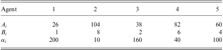
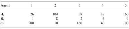
The environment. In Arifovic and Ledyard (Reference Arifovic and Ledyard2011) we used the utility functions and cost of production in Chen and Tang (Reference Chen and Tang1998) in order to compare our results to those generated with humans. The per-person cost, c, of producing a unit of the public good, which determines Z, is set to 20 and the utility parameters are given in Table 1. We consider a basic environment E with N = 5. We also consider E(10) with N = 50 and E(20) with N = 100.

Table 1

Utility parameters

The behavioral model. We used the IEL model described in the previous section. For the runs reported in this section, we set the memory capacity J = 200 and Θⁱ = [−4,6]Footnote 17. We set the rate of experimentation ρ = 0.033. Forgone utility $--><$> {{u}^i} = {{W}^i} ({{m}^i} |{{r}^i} (m),\gamma ) <$><!--$ from Equation (1). We consider both random and modified initialization.

The mechanisms. Our goal is to investigate the pattern of convergence times over a range of values of γ that includes the cut points associated with the dominant-diagonal and strategic-complementarity conditions. For our model with N = 5, the dominant-diagonal condition is satisfied for γ ⩾ 30, and the strategic-complementarity condition is satisfied for γ ⩾ 80. Thus, for N = 5, we picked γ = 10, 30, 50, 80, 100, 180, and 260.

The sufficient condition generated by a strategic-complements sufficiency condition for convergence of best-reply algorithms requires that γ be scaled linearly in N. This is also true for the dominant-diagonal condition for convergence of best-reply algorithms. Thus, for N = 50 (k = 10) and N = 100 (k = 20) we chose values of γ so that the ratio γ/k remained constantFootnote 18.

The simulations. For each mechanism, γ, we conducted R = 1000 runs. Each run, r, was terminated 100 periods after a convergence criterion was fulfilledFootnote 19. For the analysis of the behavior observed in the simulations reported in this paper, we adopt the same convergence criteria that we used in Arifovic and Ledyard (Reference Arifovic and Ledyard2011). This allows us to compare the results of simulations with ‘small’ and ‘large’ N.

Our convergence criterion is defined in terms of how close all agents’ messages are to the equilibrium messages. This convergence criterion is fulfilled when the difference between the equilibrium value and the value of the selected message of each agent is less than or equal, in absolute terms, to a positive number d; that is, when $--><$> |m_{t}^{i} \,{\rm{ - }}\,{{m}^{ie}} | \,\leqslant \,0.1 <$><!--$ for all i. In our simulations, we set d = 0.1.

3.2 Performance measures

Because we are interested in whether and how fast these mechanisms converge to the equilibrium, we use two measures of performance: (1) the time of first passage through equilibrium and (2) an index of equilibrium stability.

Time of convergence. In Arifovic and Ledyard (Reference Arifovic and Ledyard2011) the time of convergence is defined in the following way. The period when the convergence criterion is first fulfilled is called the time of the first passage through equilibrium, T ^γ,r for run r and given γ. The average time of the first passage through equilibrium for R runs, $--><$> {{\bar{T}}^\gamma }, <$><!--$ is given by:

$--><$$>\bar{T}_{c}^{\gamma } = \frac{{\mathop{\sum}\limits_{r = 1}^R {{{T}^{\gamma, r}} } }}{R}\eqno<$$><!--$

We denote the standard deviation from this value, across the R runs, by $--><$> {{\sigma }_{{{T}^\gamma } }} <$><!--$ .

Stability of convergence. In addition to recording the time when our convergence criterion is first fulfilled, we also want to find out how stable it is (as in Arifovic & Ledyard, Reference Arifovic and Ledyard2011). In other words, is the convergence criterion satisfied by accident and agents have heterogenous collections of messages, or do the collections converge towards the values of the equilibrium messages? The measure that we use (see Arifovic & Ledyard, Reference Arifovic and Ledyard2011) is based on the individual's action sets––the set of strategies from which the agents choose their messages. We call this the index of equilibrium stability in strategies S ^s. It measures the percentage of all possible choices that are close to that agent's equilibrium message.

$--><$$>{{S}^s} = \frac{{\mathop{\sum}\limits_{t = {{T}^{\gamma, r}} \, + \,1}^{{{T}^{\gamma, r}} \, + \,100} {\mathop{\sum}\limits_{i = 1}^N {\mathop{\sum}\limits_{j = 1}^J {S_{{j,t}}^{i} } } } }}{{NJ}}\eqno<$$><!--$

where $--><$> S_{{j,t}}^{i} <$><$> |a_{{j,t}}^{i} \,{\rm{ - }}\,{{m}^{ie}} |\leqslant d <$><!--$ and otherwise equals 0.

3.3 Results

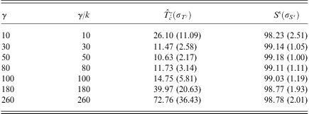
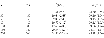
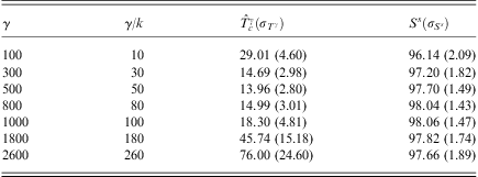
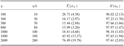
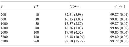
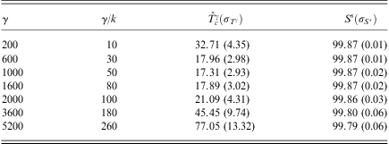
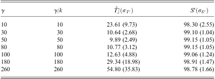
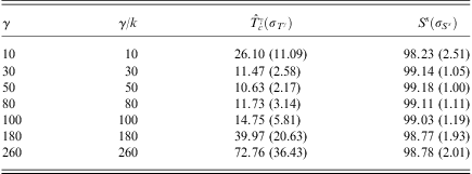
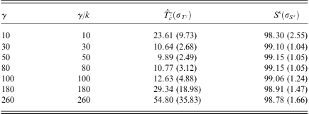
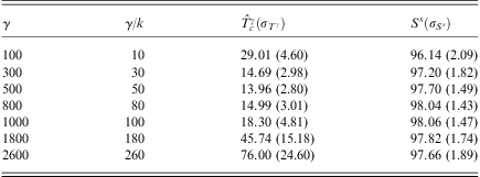
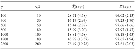
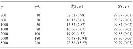
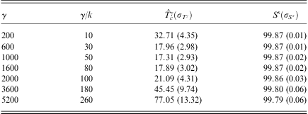
Convergence times.Tables 2–7 and Figure 1 show that increases in the number of agents do not affect the dynamics of IEL in GL games. The U-shaped feature of convergence time is preserved across 10- and 20-times increases in the number of agents. The factor γ/N = 50 remains the value that results in the minimum time to convergence.

Table 2

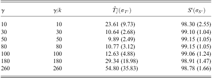
Time to convergence, N = 5, k = 1: random initialization, ρ = 0.033

Figure 1

Convergence times for different N

Overall, the times of convergence slightly increase with 10- and 20-fold increases in the number of agents. With random initialization, for each γ/k value, $--><$> \bar{T}_{c}^{\gamma } <$><!--$ increases by three to four periods as we move from N = 5 (Table 2) to N = 50 (Table 4), and then another few periods when we go from N = 50 to N = 100 (Table 6). The factor γ/N = 50 remains the value that results in the minimum time to convergence for both N = 50 and N = 100. Modified initialization results in faster convergence for N = 50 (see Table 3). However, for N = 50 and N = 100 the times of convergence are almost the same as for random initialization (see Tables 5 and 7). Figure 1 plots times to convergence for all of our values of N and for both random and modified initializations. The figure illustrates nicely how all of the U-shaped curves associated with different N's and initialization procedures are close to each other, reaching the minimum value at γ/N = 50.

Table 3

Time to convergence, N = 5, k = 1: modified initialization, ρ = 0.033

Table 4

Time to convergence, N = 50, k = 10: random initialization, ρ = 0.033

Table 5

Modified initialization, ρ = 0.033: time to convergence, N = 50, k = 10

Table 6

Time to convergence, N = 100, k = 20: random initialization, ρ = 0.033

Table 7

Time to convergence, N = 100, k = 20: modified initialization, ρ = 0.033

It is perhaps understandable that for low values of γ/K, especially below 30, the time to converge will be higher than for values between 30 and 80 since best-reply dynamics are unstable (due primarily to overreactions) and so a period of averaging is necessary to get convergence. But this does not explain the fact that $--><$> \bar{T}_{c}^{\gamma } <$><!--$ increases for high values of γ/k. As γ/k grows, there is stronger pressure for all agents to coordinate on a common value, typically not the equilibrium one, in order to minimize the difference between their own and average contribution of others. Once the coordination takes place, strategies that participated in this receive relatively high payoffs and are then copied, increasing in frequency. So, collections of strategies become homogenized. At that point, experimentation is required in order to introduce strategies close to the equilibrium ones that will get the mechanism out of the non-equilibrium outcome. However, given the circumstances, it takes time for the required experimentation to succeed. Most new values that deviate from the strategy everyone has coordinated on will most likely receive lower forgone payoffs and, thus, disappear from the collections. The larger that γ/k is, the more important this effect becomes, increasing the time to converge to equilibrium.

The values of the standard deviation of the time to converge, $--><$> {{\sigma }_{{{T}^\gamma } }} <$><$> \bar{T}_{c}^{\gamma } <$><!--$ ) and then start increasing, reaching high values for the two largest γ/k values, 180 and 260. This pattern is shared by both random and modified initialization. The standard deviations are smaller for the modified initialization than for the random initialization. The explanation for this is that all the simulations with modified initialization start out with collections of strategies that are more similar across different runs, and, thus, are likely to have more similar dynamics, and a tighter distribution of convergence times. The standard deviations decrease as N increases, a variation on the law of large numbers.

Stability. Once the IEL reaches an equilibrium, there is a high degree of stability. For all of the simulations, our measure of stability is above 96%. Again, one can notice, for N = 5 and N = 50 a slightly U-shaped pattern, with stability increasing as γ/k reaches 50, and slightly decreasing after that. Simulations with N = 100 have stability values close to 100% for all values of γ/k and for both types of initialization.

The invariance in scale. As long as we adjust γ(k) so that γ(k)/k is constant, the dynamics of IEL in GL mechanisms seem to be invariant in k. Why might this be so? We have two thoughts on this.

First, consider the standard theoretical convergence criteria based on the second-derivatives of the utility functions. Let $--><$> N = k\hat{N},\gamma = k\hat{\gamma } <$><$> \hat{\delta } = N/K = \hat{\gamma }/\hat{N} <$><$> \gamma /N\,\geqslant\,2{{B}^i} <$><$> \hat{\gamma }/\hat{N}\,\geqslant\,2{{B}^i} <$><$> \hat{\gamma }/\hat{N}\,\geqslant\,\frac{{k\hat{N}\,{\rm{ - }}\,2}}{{k\hat{N}\,{\rm{ - }}\,1}}B <$><$> \hat{\gamma }/\hat{N}\,\geqslant\,B <$><!--$ , which is also scale independent.

Second, consider the utility payoff to any agent. It is symmetric around the best reply. Since IEL is picking messages that are on average in proportion to utility, then IEL is picking randomly around best reply. So on average IEL will be picking the best reply. Let us see what that means as k→∞. For quadratic utility functions, the best reply is $--><$> m = \frac{{{\rm{ - }}(A\,{\rm{ - }}\,c)\, + \,[(\gamma /N)\, + \,2B](N\,{\rm{ - }}\,1)\mu }}{{(\gamma /N)[(N\,{\rm{ - }}\,1)\,{\rm{ - }}\,2NB]}} <$><$> m = \left[ {{\rm{ - }}\frac{1}{{N\,{\rm{ - }}\,1}}({{A}^i} \,{\rm{ - }}\,c)\, + \,(\hat{\delta }\, + \,2B)\mu } \right]/\left[ {\hat{\delta }(1\,{\rm{ - }}\,2(\frac{{k\hat{N}}}{{k\hat{N}\,{\rm{ - }}\,1}})B)} \right] <$><$> m = {\rm{ - }}\phi \, + \,\psi \mu <$><$> \phi = {\rm{ - }}(A\,{\rm{ - }}\,c)/[k\hat{N}\hat{\delta }(1\,{\rm{ - }}\,2B)] <$><$> \psi = [\hat{\delta }\, + \,2B]/[\hat{\delta }(1\,{\rm{ - }}\,2B)] <$><$> k{{\mu }_{t{\rm{ - }}1}} = \frac{k}{{k\hat{N}\,{\rm{ - }}\,1}}({{\hat{x}}_{t{\rm{ - }}1}}\,{\rm{ - }}\,{{m}_{t{\rm{ - }}1}})\, \rightarrow \,{{x}_{t{\rm{ - }}1}} <$><$> km_{t}^{i} \, \rightarrow \,\frac{{A\,{\rm{ - }}\,c}}{{\left( {{{\hat{\delta }} \mathord{\left/ {\vphantom {{\hat{\delta }} {\hat{N}}}} \right. \kern-\nulldelimiterspace} {\hat{N}}}} \right)(1\,{\rm{ - }}\,2B)}} + \left[ {\frac{{\hat{\delta }\, + \,2B}}{{\hat{\delta }(1\,{\rm{ - }}\,2B)}}} \right]{{x}_{t{\rm{ - }}1}} = {{\phi }^i} \, + \,{{\psi }^i} {{x}_{t{\rm{ - }}1}} <$><$> {{x}_t} = \left[ {\mathop{\sum}\nolimits_{i = 1}^{\hat{n}} {{\phi }^i} } \right]\, + \,\left[ {\mathop{\sum}\nolimits_{i = 1}^{\hat{n}} {{\psi }^i} } \right]{{x}_{t{\rm{ - }}1}} <$><$> \hat{\delta } <$><!--$ constant.

The impact of the modified initialization. Based on our work with N = 5, we expected the modified initialization to lead to faster times of convergence. But, instead, for N = 50 and N = 100 the convergence times are pretty much the same for random and modified initializations. There is an explanation for this.

As described in the previous section, we start the modified initialization by randomly drawing J rules for each agent i. Then for each rule j, we randomly draw 100 values of μ_−jk in [−4,6] and 100 values of $--><$> \sigma _{{{\rm{ - }}jk}}^{2} <$><$> \upsilon_{j}^{i} = (1/100)\mathop{\sum}\nolimits_k {{u}^i} (\theta _{j}^{i} |{{r}_{{\rm{ - }}jk}}) <$><$> \sigma _{{{\rm{ - }}i}}^{2} <$><$> \sigma _{{{\rm{ - }}i}}^{2} <$><!--$ does not matter at all, and only the expected value of μ_−i = l plays a role. So (with some randomness) our initialization essentially computes the best response to μ_−i = 1. So the closer the expected value of μ_−i is to its equilibrium value, the faster convergence will be.

The precise calculation of the equilibrium value of μ_−i is

$--><$$>{{\mu }_{{\rm{ - }}i}} = \frac{{\hat{X}\,{\rm{ - }}\,{{{\hat{m}}}^i} }}{{N\,{\rm{ - }}\,1}} = \frac{1}{{5k}}\left\{ {\hat{X}\,{\rm{ - }}\,\frac{1}{{\hat{\gamma }(5k\,{\rm{ - }}\,1)}}\left[ {{{A}^i} \,{\rm{ - }}\,2{{B}^i} \hat{X}\,{\rm{ - }}\,c} \right]} \right\}\eqno<$$><!--$

For N = 5 and γ = 10, the equilibrium values of μ_−i are 1.1, 0.9, 1.05, 0.95, and 1. Fixing N, as γ/k grows, the equilibrium value of μ_−i goes to $--><$> \hat{X}/N <$><$> \gamma = k\hat{\gamma } <$><!--$ , as k grows the equilibrium values of μ_−i go to zero. This means that the expected value of μ_−i drawn in the initialization is moving further away from its equilibrium value. For k = 10, N = 50, and γ/k = 50, the equilibrium values of μ_−i are near 0.1, and for k = 20 they are near 0.05. That is, they are approximately 1/k of the value for N = 5. So the advantage that modified initialization has for N = 5 is seriously eroded as k grows.

This intuition also helps explain why the variance of convergence times is lower for modified than for random. Modified starts out at about the same place each time, whereas random starts from many different places. On average they take the same time (since, on average, random also starts at μ_−i = 1) but sometimes random is closer and sometimes it is not.

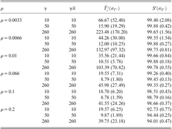
The impact of an increase in the rate of experimentation. We conducted a set of simulations with random initialization and a rate of experimentation for ρ = 0.066. The higher rate of experimentation, twice as high as in our baseline simulations, resulted in somewhat faster convergence times. On average, for each γ/k, convergence is by three to four periods faster compared with the simulations with ρ = 0.033. We illustrate the results, for N = 5 and random initialization in Table 7. It is interesting to note that relatively high rate of experimentation does not introduce disruption that might slow down or prevent convergence. Instead, it speeds things up. The reason for this is the fact that new values generated via experimentation are not played out right away. They first have to prove, in terms of forgone payoffs, that they might be worthwhile candidates. If they do so, then, through imitation, they increase in frequency and thus increase their chances to be selected as actual messages. Otherwise, new values with relatively low forgone payoffs quickly disappear from the collections (See Table 8 for times to convergence for $--><$>\rho = 0.066<$><!--$ ).

Table 8

Time to convergence, N = 5, k = 1: random initialization, ρ = 0.066

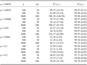
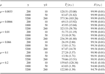
Variation in the rate of experimentation. The behavior observed in case of a twice-as-high rate of experimentation as our baseline case, for N = 5, made us curious about the robustness of our large N system with respect to a wide range of rates of experimentation. Thus, in addition, we simulated the system for the following values of ρ: 0.0033, 0.0066, 0.01, 0.066, 0.1, and 0.2. Again, we used the same values of γ/k equal to 10, 30, 50, 80, 100, 180, and 260. We report the results (which are the averages over R = 1000 runs in Tables 9 (for N = 5), Table 10 (for N = 50), and Table 11 (for N = 100)). For brevity, we report the results for γ/k = 10, 50 and 260 only. Our results show that the U-shaped pattern of behavior is preserved regardless of the rate of experimentation. They also show that very low rates, such as 0.0033 and 0.0066, result in slower convergence. However, there is a difference between the two. The rate of ρ = 0.0033 results in the highest average times of convergence. These averages decrease almost in half for ρ = 0.0066.

Table 9

Different rates of experimentation, time to convergence, N = 5, k = 1

Table 10

Different rates of experimentation, time to convergence, N = 5, k = 10

Table 11

Different rates of experimentation, time to convergence, N = 100, k = 20

For N = 5, higher rates of experimentation of 0.1 and 0.2 do not have much of an impact on the times to convergence compared with our baseline case. In addition, for N = 50 and N = 100, the higher rates of experimentation of ρ = 0.066 and 0.1 do not have much impact on the average times to convergence compared with the baseline case with ρ = 0.033. However, a high rate of experimentation, ρ = 0.2, results in somewhat higher values of the average times to convergence. The effects of this high rate of experimentation are stronger in case of N = 100. Note that the qualitative features of the behavior are still preserved even when the collection of strategies undergo this fairly large experimentation, with 20% turnover in each time period. Finally, it is worthwhile to note that a relatively high rate of experimentation of 0.2 still does not affect the stability once the convergence occurs. For all N the stability goes down by few percentage points, but remains well above 90%.

3.4 Comparison with other models of learning

A number of models of individual learning have been developed over the past decade. (For an excellent overview, see Camerer, Reference Camerer2003). Much of the research has been done in the context of one-shot games with small strategy spaces such as 2-by-2 or 3-by-3 games. The performance of the models has generally been evaluated by using standard econometric methods (maximum likelihood or grid search) to fit the models to experimental data. Two of the most frequently used models from this strand of literature are the Reinforcement Learning (RL) (Erev & Roth, Reference Erev and Roth1998) and the Experience-Weighted Attraction (EWA) Learning (Camerer & Ho, Reference Camerer and Ho1999).

The implementation of both algorithms requires either that all possible players’ strategies are enumerated, that is, explicitly represented in the collection, or that the strategy space is discretized. In RL, strategies that achieve higher returns when used are reinforced and played with a higher probability. In EWA, each strategy has an attraction based on the possible payoff it might have earned had it been played in the past. Strategies with higher attractions have higher probabilities of being selected. One of the primary differences between RL and EWA is the latter's use of hypothetical computations to quickly evaluate all strategies. RL only uses actual payoffs and thus can only evaluate strategies that have actually been played.

What is common to RL and EWA on one hand, and IEL on the other, is that all of them update the collections of their strategies in such a way that the frequencies of those that have performed well increase over time. The choice of a particular strategy as the actual strategy that a player uses in a given period is probabilistic, and the strategies’ selection probabilities depend positively on their past performance.

The differences between IEL, on one hand, and RL and EWA on the other, stem from the way that the strategy sets (collections) are determined and updated. IEL starts out with a set of randomly generated strategies (messages). It brings in new strategies to be tried via experimentation. The way experimentation is implemented allows IEL, unlike RL and EWA, to handle large strategy spaces well. For example, in the GL mechanism, each agent has a continuum of possible messages. In order to apply models such as RL and EWA, the continuum must be discretized. However, discretization causes problems when there are very fine differences in equilibrium values between different mechanisms. IEL handles that problem well. It does start out with randomly chosen sets of alternatives for each agent, but due to directed experimentation there is a sufficiently high probability that any important omitted messages, such as the Nash Equilibrium messages, will be added to the set.

IEL adds a new dimension to RL and EWA by allowing agents to vary their active strategy set in response to experience. What has been ‘learned’ by an agent at any time is summarized not in attraction weights but in the set of active strategies. Strategies that have been or would have been successful will have more copies in the active strategy set. If a strategy has a lot of copies in the active set, it will be chosen with a higher probability. The primary difference between IEL and RL and EWA seems to be that IEL discards strategies that aren't potentially profitable and thus does not waste time or lose payoffs re-testing unprofitable options. (See Arifovic and Ledyard (Reference Arifovic and Ledyard2004) for the comparison of the performance of RL, EWA, and IEL in the GL mechanisms. Also, see Arifovic and Ledyard (Reference Arifovic and Ledyard2009) for comparison of the performance of IEL and EWA in a voluntary contribution mechanism.)

4 Final remarks

In Arifovic and Ledyard (Reference Arifovic and Ledyard2011), we investigated IEL's behavior in a class of games with a small number of agents. The number of agents in that setup was equal to five in order to match the design and the number of human subjects who participated in the laboratory experiments. Both IEL simulations and experiments were conducted for a number of different values of the free parameter of the model. Our results showed that IEL successfully captures and predicts the behavior observed in the experiments with human subjects. We have also successfully applied our behavioral model in the context of the call markets where the IEL model generates the same types of price volatility and efficiencies as those generated in our experiments with human subjects (Arifovic & Ledyard, Reference Arifovic and Ledyard2011), and to the voluntary provision of public goods environment where our model matches the patterns of behavior of the average contribution over time from a number of different human subjects experiments (Arifovic & Ledyard, Reference Arifovic and Ledyard2011). This collection of results suggests that we can use our behavioral model as a computer testbed to study a number of mechanism design issues such as out-of-equilibrium behavior, speed of convergence, efficiency, price volatility, and the stability of equilibria.

Thus, in this paper, we used this methodology to investigate what happens with GL mechanisms in linear public-good environments when the number of agents, N, becomes large. Testbeds of this scale are not easily implemented in the controlled laboratory setting with human subjects. Our findings are interesting. The main features of the behavior observed with the small number of agents are preserved when γ is scaled by the multiplicative factor k. For a given γ/k, the average times to convergence are similar. Further, the U-shaped pattern arising from variations in the value of γ/k is preserved. This result is robust to implementation of a wide range, low and high, of rates of experimentation. The advantage of IEL over other models of individual learning, such as RL and EWA Learning is that it can handle large strategy spaces well.

Acknowledgments

We thank Olena Kostyshyna for her very able research assistance. We also thank an anonymous referee for very helpful comments.

Footnotes

¹ These will be defined more precisely later.

² This section is intended mainly as a reminder to the reader of the formal structure of the problem. For more details, see Groves and Ledyard (Reference Groves and Ledyard1977) or Chen and Plott (Reference Chen and Plott1996).

³ Adaptive learning is defined in Milgrom and Roberts (Reference Milgrom and Roberts1990) and includes best response, fictitious play, Bayesian Learning, and others. The sufficient condition for convergence under adaptive learning is $--><$>{{\partial }^2} {{V}^{_{i} }} /\partial {{m}^{_{i} }} \partial {{m}^{_{j} }} \,\geqslant \,0 <$><!--$ .

⁴ We thank Paul Healy for the Gabay–Moulin reference. See Healy (Reference Healy2006) for a use of the theorem in the context of public good mechanism design. The diagonal condition is satisfied if $--><$> |{{\partial }^2} {{W}^{_{i} }} /\partial {{m}^{_{i} }} {{m}^{_{i} }} | \gt \,\mathop{\sum}\nolimits_{i \ne j} |{{\partial }^2} {{W}^{_{i} }} /\partial {{m}^{_{i} }} {{m}^{_{j} }} | <$><!--$ .

⁵ This follows from the Gabay–Moulin condition since the left-hand side of the inequality goes to zero as $--><$> N \rightarrow 0 <$><!--$ , while the right-hand side is bounded away from zero.

⁶ It can be shown that $--><$>{\ lim }_{k \rightarrow \infty } \,{{u}^i} (\hat{m}(kN\hat{\gamma }))\,{\rm{ - }}\,{{u}^i} (\hat{m}(kN\hat{\gamma })/{{\mu }_{{\rm{ - }}i}}) = 0 <$><!--$ .

⁷ See Watkins (Reference Watkins1989).

⁸ A number of applications in economics use the genetic algorithm (developed by Holland, Reference Holland1970, Reference Holland1974) to implement this idea. For example, see Arifovic (Reference Arifovic1996), Miller (Reference Miller1996), Marks (Reference Marks1998), Vriend (Reference Vriend2000), Lux and Schonstein (Reference Lux and Schornstein2005), etc.

⁹ Our approach follows most closely Arifovic (Reference Arifovic1994), but there have been a number of other individual learning applications, for example, Marimon et al. (1990), Vriend (Reference Vriend2000), Lux and Hommes (Reference Hommes and Lux2008).

¹⁰ Since we use the identical algorithm that we used for our simulations with N = 5, our description closely follows the behavioral model presented in Arifovic and Ledyard (Reference Arifovic and Ledyard2011).

¹¹ J is a free parameter of IEL. In this paper we set J = 200.

¹² ρ is a free parameter of the behavioral model. In this paper we set ρ = 0.033, exactly the same number we have used in our other IEL papers.

¹³ An alternative selection model is the probabilistic choice function $--><$>\pi ({{\theta }^k} ) = {{{{e}^{\lambda {{u}^i} ({{\theta }^k} )}} }}/{{\mathop{\sum}\nolimits_j {{e}^{\lambda {{u}^i} ({{\theta }^k} )}} }} <$><!--$ . We have found (see e.g. Arifovic & Ledyard, Reference Arifovic and Ledyard2011) that the behavior predicted changes very little with this model from our proportional selection rule, for all λ. This is because the set A tends to become homogeneous fairly fast, at which point the selection rule is irrelevant.

¹⁴ This implies that if there are negative forgone utilities in a set, payoffs are normalized by adding a constant to each payoff that is, in absolute value, equal to the lowest payoff in the set.

¹⁵ See Camerer and Chong (Reference Camerer and Chong2004).

¹⁶ Our subjects were given a ‘what-if’ calculator that they could use prior and during the beginning of an experiment. Chen and Tang's subjects did not have access to such a tool.

¹⁷ This was the range of values used in the both the Arifovic–Ledyard and Chen-Tang experiments.

¹⁸ It is worth pointing out that we use our learning algorithm to ‘locate’ equilibria. This is different from for solving for an evolutionary stable equilibrium, where one takes an existing equilibrium and asks whether it is stable with respect to best-response dynamics. We thank our anonymous referee for this remark.

¹⁹ The maximum number of periods for each run was set at t_max = 1000. If the convergence criterion is not fulfilled by that time, a run is terminated. All of our runs, for all γ's and N's converged within 1000 periods.

References

Arifovic, J. 1994. Genetic algorithm learning and the cobweb model. Journal of Economic Dynamics and Control 18, 3–28.CrossRef Google Scholar

Arifovic, J. 1996. The behavior of the exchange rate in the genetic algorithm and experimental economies. Journal of Political Economy 104, 510–541.CrossRef Google Scholar

Arifovic, J., Ledyard, J. 2004. Scaling up learning models in public good games. Journal of Public Economic Theory 6, 205–238.CrossRef Google Scholar

Arifovic, J., Ledyard, J. 2009. Individual Evolutioanry Learning and the Voluntary Contributions Mechanisms. manuscript.Google Scholar

Arifovic, J., Ledyard, J. 2011. A behavioral model for mechanism design: Individual Evolutionary Learning. Journal of Economic Behavior and Organization 78, 374–395.CrossRef Google Scholar

Camerer, C., Ho, T. 1999. Experience weighted attraction learning in normal form games. Econometrica 67, 827–873.CrossRef Google Scholar

Camerer, C. F. 2003. Behavioral Game Theory: Experiments in Strategic Interaction. Princeton University Press.Google Scholar

Camerer, C., Chong, J. 2004. A cognitive hierarchy model of games. The Quarterly Journal of Economics 119, 861–898.CrossRef Google Scholar

Chen, Y., Plott, C. 1996. The Groves–Ledyard mechanism: an experimental study of institutional design. Journal of Public Economics 59, 335–364.CrossRef Google Scholar

Chen, Y., Tang, F. 1998. Learning and incentive compatible mechanisms for public goods provision: an experimental study. Journal of Political Economy 106, 633–662.CrossRef Google Scholar

Erev, I., Roth, A. 1998. Predicting how people play games: reinforcement learning in experimental games with unique, mixed strategy equilibria. American Economic Review 80, 848–881.Google Scholar

Gabay, D., Moulin, H. 1980. On the uniquencess and stability of Nash equilibria in noncooperative games. In Appliced Stochastic Control in Econometrics and Management Science, Bensoussan, A., Kleindorfer, P.S., & Tapiero, C.S. (eds), North-Holland, Amsterdam, pp. 271–293.Google Scholar

Groves, T., Ledyard, J. 1977. Optimal allocation of public goods: a solution to the ‘Free Rider’ problem. Econometrica 45, 783–809.CrossRef Google Scholar

Healy, P. 2006. Learning dynamics for mechanism design: an experimental comparison of public goods mechanisms. Journal of Economics Theory 129, 114–149.CrossRef Google Scholar

Holland, J.H. 1970. Robust algorithms for adaptation set in a general formal frameowork. Proceedings of the IEEE Symposium on Adaptive Processes, Decision and Control 17, 51–55.Google Scholar

Holland, J. H. 1974. Adaptation in Natural and Artificial Systems. University of Michigan Press.Google Scholar

Hommes, C., Lux, T. 2008. Individual Learning, Heterogeneity and Aggregate Behavior in Cobweb Experiments. Manuscript.Google Scholar

Lux, T., Schornstein, S. 2005. Genetic learning as an explanation of stylized facts of foreign exchange markets. International Journal of Mathematical Economics 41, 169–196.CrossRef Google Scholar

Marimon, R., McGrattan, E., Sargent, T.J. 1990. Money as a medium of exchange in an economy with artificially intelligent agents. Journal of Economic Dynamics and Control 14, 329–373.CrossRef Google Scholar

Marks, R. E. 1998. Evolved perception and behavior in oligopolies. Journal of Economic Dynamics and Control 22, 1209–1233.CrossRef Google Scholar

Milgrom, P., Roberts, J. 1990. Rationalizability, learning, and equilibrium in games with strategic complementarities. Econometrica 58, 1255–1277.CrossRef Google Scholar

Miller, J. 1996. The coevolution of automata in the repeated prisonner's dilemma. Journal of Economic Behavior and Organization 29, 87–112.CrossRef Google Scholar

Muench, T., Walker, M. 1983. Are Groves–Ledyard equilibria attainable? The Review of Economic Studies 50, 393–396.CrossRef Google Scholar

Page, S., Tassier, T. 2004. Equilibrium selection and stability for the Groves–Ledyard mechanism. Journal of Public Economic Theory 6, 311–335.CrossRef Google Scholar

Vriend, N. 2000. An illustration of the essential difference between individual and social learning and its consequences for computational analyses. Journal of Economic Dynamics and Control 24, 1–19.CrossRef Google Scholar

Watkins, C. 1989. Learning from Delayed Rewards. University of Cambridge.Google Scholar