The Formation of Large Villages

According to Schlanger and Craig, before AD 500 “there were no large settlements—settlements reaching the 75–100 person threshold” anywhere in the Southwest/Northwest (Reference Schlanger, Craig, Young and Herr2012:199). Over the next five centuries, villages of several hundred people appeared. In AD 700, for example, the largest Hohokam villages may have had “a peak momentary population between 400 and 600” (Craig et al. Reference Craig, Wallace, Lindemann, Young and Herr2012:50). In the late 800s the population of one of those villages, the Grewe site, may have approached 1,000 people (Craig Reference Craig and Craig1999:146). Larger villages also formed in the northern Southwest/Northwest (e.g., Varien et al. Reference Varien, Ortman, Kohler, Glowacki and Johnson2007; Wilshusen and Ortman Reference Wilshusen and Ortman1999) but did not last. Whether transitory or long-lived, the newly emerged larger villages were exceptions in landscapes dominated by small residential sites (e.g., Young and Herr Reference Young and Herr2012). In some cases, clusters of habitations indicate communities of perhaps 200 to 300 individuals—the equivalent of small villages but often with wide spacing between households.

After AD 1000, the Puebloans in the northern part of the region built increasingly large villages that usually consisted of tightly packed, apartment-like dwellings; as Rautman (Reference Rautman2000) puts it, aggregation was accompanied by “nucleation.” Hill and colleagues (Reference Hill, Clark, Doelle and Lyons2004) and Mills, Peeples, and colleagues (Reference Mills, Peeples, Haas, Borck, Clark and Roberts2015) refer to the process as “community coalescence” to highlight social aspects of village formation including the amalgamation of disparate groups. By whatever name, the process began before AD 1300 but accelerated afterward. In the case of the Puebloans,

We can gain a sense of usual village size (as opposed to maximum size) from Ortman's (Reference Ortman and Spielmann1998) data on 136 sites from the Puebloan region, occupied both before and after AD 1300. For the Pueblo III period (AD 1150–1300), Ortman documents 4,217 structures at 97 sites, with a mean of 43 structures per site. For the Pueblo IV period (AD 1300–1540), he documents 16,941 structures in 29 sites, or 584 structures per site. If the number of structures is a proxy for population, the average Pueblo IV village in Ortman's sample held more than 10 times the population of Pueblo III villages.

Although Hohokam villages in southern Arizona were less nucleated than their Puebloan counterparts, settlements of 1,000 or more persons were common in the Phoenix Basin after AD 1250, and aggregation occurred at a smaller scale in adjacent valleys and basins (Hill et al. Reference Hill, Wilcox, Doelle and Robinson2012). The process is apparent even in smaller drainages such as the northern San Pedro Valley, where the roughly 1,200 inhabitants lived in numerous farmsteads and hamlets in the 1100s and early 1200s and then moved into a dozen walled villages in the late 1200s (Clark and Lyons Reference Clark and Lyons2012; Hill et al. Reference Hill, Clark, Doelle and Lyons2004:Figure 7).

Lifeways, Territorial Abandonment, and Population Loss

The lifeways involving large nucleated settlements were also embraced by the Mimbres, Casas Grandes, Jornada Mogollon, the Prescott Branch, and the Fremont culture. Today's Pueblo Indian villages occur in far fewer places. When the Spanish arrived they noted the ruins of former villages in areas that were no longer permanently occupied.

In southern Arizona, the 1300s were characterized by large villages, territorial contraction, and a “retreat from interstitial areas” (Abbott et al. Reference Abbott, Breternitz, Robinson and Abbott2003:5), opening up buffer zones between settlement clusters (Wilcox et al. Reference Wilcox, Robertson, Wood, Rice and LeBlanc2001). Demographic decline began during the early 1300s, continued into the early 1400s, and was more dramatic than that experienced in the Puebloan world (Hill et al. Reference Hill, Clark, Doelle and Lyons2004:Figure 4). At least some groups returned to living in pit houses before becoming archaeologically invisible (or nearly so) by AD 1450 (e.g., Chenault Reference Chenault, Doyel, Fish and Fish2000; Craig Reference Craig2011; Marshall Reference Marshall2009).

The dramatic shrinkage in regional occupation is a key unresolved issue in Southwest/Northwest archaeology. Early efforts to explain that shrinkage focused on single causes, but it is now clear that the contraction of settlement was a complex process that took centuries and ended only in modern times. Specific factors such as climate change or warfare played a role at a local scale, and population decrease at that scale can be seen as part of “ordinary” demographic ebb and flow (e.g., Hill et al. Reference Hill, Lyons, Clark and Doelle2015; Schwindt et al. Reference Schwindt, Kyle Bocinsky, Ortman, Glowacki, Varien and Kohler2016). The issue is not local abandonments per se but the progressive emptying of the regional landscape: after AD 1300, most depopulated areas were not recolonized. Following Dorigo and Tobler (Reference Dorigo and Tobler1983), archaeologists suspect the existence of “pull” factors—drawing people to certain areas and keeping them there—as well as of “push” factors that made areas less desirable or untenable (e.g., Cameron Reference Cameron1995; Glowacki Reference Glowacki2015).

Eight decades ago, Harold Colton argued that “the population of Northern Arizona increased seven fold between 600 A.D. and 1100 A.D. . . . During the next eight hundred years . . . the population decreased. This decrease was equal to the previous gain” (Reference Colton1936:343). Nonetheless, migration (e.g., Cameron Reference Cameron1995; Kunitz and Euler Reference Kunitz and Euler1972:3–7; Spielmann Reference Spielmann1998) boosted some local populations at the expense of others, so it was not clear that instances of local depopulation meant a drop in total population. As more data became available, however, suspicions were confirmed that a substantial population drop began before the introduction of Old World diseases (Dean et al. Reference Dean, Doelle, Orcutt and Gumerman1994; Doelle Reference Doelle and Dean2000).

Any lingering doubts were diminished by the Coalescent Communities Database (CCD), a collaborative project whose goal was to identify sites, estimate total room counts, and establish occupation spans for all settlements in the Southwest/Northwest with more than 12 rooms and dated between AD 1200 and 1500 (Hill et al. Reference Hill, Clark, Doelle and Lyons2004; Hill et al. Reference Hill, Wilcox, Doelle and Robinson2012; Wilcox et al. Reference Wilcox, Doelle, Brett Hill and Holmlund2003). While numerous demographic shifts (including migrations) are indicated by population density contour maps generated from the CCD (Hill et al. Reference Hill, Clark, Doelle and Lyons2004:Figure 3), two panregional trends are evident: population concentration from AD 1250–1300 onward and population decline that began between AD 1300 and 1350 and continued to European contact (Hill et al. Reference Hill, Clark, Doelle and Lyons2004:Figures 2, 4). The severity of the decline indicated by architectural reconstructions is still a contested issue, especially in the southern Southwest, where surviving groups dispersed into small pit house settlements in the late 1300s (Chenault Reference Chenault, Doyel, Fish and Fish2000). However, nearly all of the well-documented late settlements were depopulated during the 1400s, before the arrival of Europeans (e.g., Craig Reference Craig2011; Marshall Reference Marshall2009).

The Southwest Social Networks (SWSN) project then added existing ceramic and obsidian sourcing data to the portion of the CCD west of the Continental Divide, in order to examine regional social networks (Mills, Clark, et al. Reference Mills, Clark, Peeples, Haas, Roberts, Hill, Huntley, Borck, Breiger, Clauset and Shackley2015; Mills, Peeples, et al. Reference Mills, Peeples, Haas, Borck, Clark and Roberts2015). While the SWSN added many sites to the CCD and adjusted population estimates for specific areas (Hill et al. Reference Hill, Wilcox, Doelle and Robinson2012), the two basic trends—population concentration followed by decline—were unchanged. Combined with other projects that take into account longer time spans and other data sources (e.g., Dean et al. Reference Dean, Doelle, Orcutt and Gumerman1994; Doelle Reference Doelle and Dean2000; Kohler and Reese Reference Kohler and Reese2014), the CCD and SWSN demonstrate that the Southwest/Northwest experienced “more than one thousand years of sustained population growth, a brief stasis, and beginning in the early 1300s, a striking decline in overall population” (Clark et al. Reference Clark, Brett Hill and Lyons2003:1).

At first, the Rio Grande region appears to be an exception; due to immigration beginning in the 1200s, the Spanish found a large cluster of Pueblo villages. But a more detailed look suggests that it, too, suffered precontact population loss. In the Tewa Basin, “the overall population . . . declined gradually between the middle decades of the 1400s and 1600” (Ortman Reference Ortman2016:113). And as Barrett remarks, “The explorers’ reports reveal that some parts of the Rio Grande Pueblo Region were uninhabited even though archaeological evidence establishes the existence of substantial settlement in these areas not many decades earlier” (Reference Barrett2002:49).

The Neolithic Demographic Transition

The best context for this essay is the Neolithic Demographic Transition (NDT), proposed by Jean-Pierre Bocquet-Appel (Reference Bocquet-Appel2002) based on skeletal data from Europe and North Africa. As the Neolithic lifeway spread across the region, farming led to an increase in the birth rate and thus in population. After several centuries mortality also increased, returning the growth rate to modest levels and completing the NDT (Bocquet-Appel Reference Bocquet-Appel2002, Reference Brew2008).

The NDT has since been detected elsewhere (Bocquet-Appel and Bar-Yosef Reference Bocquet-Appel and Bar-Yosef2008), confirming the utility of the concept but also showing that it played out in different places in different ways (e.g., Lesure et al. Reference Lesure, Martin, Bishop, Jackson and Chykerda2014; Schlanger and Craig Reference Schlanger, Craig, Young and Herr2012). Kohler and colleagues (Reference Kohler, Glaude, Bocquet-Appel and Kemp2008) applied the concept in a collaborative effort known as the Village Ecodynamics Project, focused on southwest Colorado and northern New Mexico. There, the regional crude birth rate reached and maintained a high level between AD 500 and 1300. After that, the crude birth rate declined rapidly across the Southwest.

By AD 800 the estimated population of the Southwest/Northwest was about 50,000; by AD 1200 it had doubled (Hill et al. Reference Hill, Clark, Doelle and Lyons2004:Figure 2; Hill et al. Reference Hill, Wilcox, Doelle and Robinson2012). During those years the average annual population growth, relative to the year before, was 0.17%. In AD 1325 the Southwest/Northwest population peaked at about 160,000; over the previous 125 years, average annual population growth was 0.38%, roughly double the rate of increase for the period before. Between AD 1325 and 1550 (the final period before significant exposure to European diseases), the regional population declined to about 75,000, an average annual population decrease of 0.34%. Comparing the rates before and after AD 1325, the end of the regional NDT involved a shift in the annual rate of population change of −0.71%.

These population estimates can no doubt be refined. However, they show that we do not need catastrophes to explain regional population decline after AD 1325. Instead we can look to processes such as those implicated in the NDT.

Village Formation and Disease

Bocquet-Appel (Reference Bocquet-Appel2002:647) has argued that the substantial increase in mortality at the end of the NDT was due to zoonoses and the clustering of individuals into villages. The concept that Neolithic village life could be unhealthy is an old one but receives little attention—no doubt because it is difficult to find direct archaeological evidence of disease (see Fink Reference Fink and Breternitz1991:75–77). Past considerations of epidemics among Native Americans usually began with the introduction of European pathogens, whose impacts can be estimated from written records (e.g., Barrett Reference Barrett2002; Ramenofsky Reference Ramenofsky1987; Reff Reference Reff1991). Nonetheless, we cannot discount precolumbian epidemics simply because it is difficult to identify them.

So far there is no evidence that Old World pathogens leaked to the New World before the Columbian exchange. There is no shortage of New World Alternatives, albeit the list varies from source to source (e.g., Aufderheide and Rodríguez-Martín Reference Aufderheide and Rodríguez-Martín1998; Martin and Goodman Reference Martin and Goodman2002). Dysentery and diarrhea (many authors use the two terms interchangeably) are a special concern. Susan Kent remarks,

In examining the ancient Hohokam of southern Arizona, many of whom depended heavily on irrigation canals for domestic water as well as agriculture, Michael Fink (Reference Fink and Breternitz1991) pointed to contaminated water as a source of disease. His (Reference Fink and Breternitz1991:Tables 5.1–5.3) lists of diseases possibly spread in canal and reservoir water include eight caused by bacteria, five caused by viruses, and five caused by intestinal worms. Fink's point was made just as forcefully, if less systematically, by Harold Colton:

As Kunitz and Euler (Reference Kunitz and Euler1972) discuss, Colton's attempts to link disease and depopulation were met with skepticism (e.g., Brew Reference Brew1946:299). Echoing earlier critiques, readers may ask whether those diseases were in place from the beginning. If so, wouldn't they have prevented populations from growing in the first place?

The answer to such objections lies in the medically established concept of “emerging infectious diseases,” or EIDs (e.g., Metcalf and Lessler Reference Metcalf and Lessler2017). Such diseases can be caused by a new pathogen, but “most emerging infections appear to be caused by pathogens already present in the environment, brought out of obscurity or given a selective advantage by changing conditions” (Morse Reference Morse1995:9). The “changing conditions” usually consist of human actions and the consequences of those actions (Engering et al. Reference Engering, Hogerwerf and Slingenbergh2013). By drawing on the mathematics of epidemiology, we can show how the formation of large villages could have triggered EIDs and thus depopulation. In turn, demographic ebb and flow across the regional landscape would have been disrupted because the surviving population was insufficient to recolonize areas after temporary local setbacks such as resource depletion or crop failures. With spatial shifts now involving more ebb than flow, and as long as large villages were the preferred mode of settlement, the result would be geographic contraction.

The next sections of this essay show that EIDs are a plausible cause of the observed late prehistoric demographic collapse in the Southwest/Northwest because they could have been triggered by aggregation into large villages and by the connections among those villages.

Approach

Users of mathematical models must decide whether the goal is (1) to replicate documented trajectories or (2) to gain insights. In the former case, models can become fairly elaborate as the creators match target events with increasing accuracy and detail (e.g., Kohler et al. Reference Kohler, Glaude, Bocquet-Appel and Kemp2008). This essay pursues the latter goal. If the epidemiological models are kept simple, those not previously exposed to them will find it easier to follow our arguments. The simulations were written in the R programming language (R Core Team 2017), which can be executed using (RStudio Team 2017), both downloadable for free; the code is preserved in tDAR: The Digital Archaeological Record (Phillips et al. Reference Phillips, Wearing and Clark2017) so that readers can replicate or modify our results.

Transmission processes in epidemics can be density-dependent or frequency-dependent (Keeling and Rohani Reference Keeling and Rohani2008). In the former approach, the intensity of human contact increases with the size of the community; in the latter approach it does not. Epidemiologists often model the spread of disease among hundreds of thousands or millions of people, and in those cases a frequency-dependent approach makes sense, but late prehistoric villages in the Southwest/Northwest probably never exceeded about 3,000 individuals. Moreover, villagers lacked preventive measures inspired by a germ theory of disease. At such population levels, and given such behavior, density-dependent models are appropriate.

Epidemiological models can be deterministic or stochastic. Deterministic models are useful for purposes of illustration and also indicate what we can expect on average. Because stochastic effects become less important with large populations, deterministic models can work well for modern studies. Nonetheless, deterministic models fail to capture two small-scale effects of interest here: the local extinction of pathogens and their failure to be transmitted among subgroups within a population.

Some models examine how demography (including birth and death) affects epidemics. Adding demography can help explain the long-term history of a specific disease. In most of our approximations, however, the goal is to model processes corresponding to a disease spreading through a village or villages over months rather than generations.

Finally, epidemiologists define various families of disease processes, using a paradigm that divides the population into subclasses according to infection status. Two basic processes are known as SIR (for Susceptible-Infectious-Recovered with immunity) and SIS (for Susceptible-Infectious-Susceptible). We chose to use both SIR and SIS models, as each is a model that corresponds to a different group of potentially relevant pathogens (see Keeling and Rohani Reference Keeling and Rohani2008:16–26, 39).

A Zero-Order Approximation Using an SIR Model

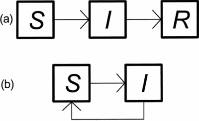
We begin by modeling diseases where recovery conveys immunity—measles is a good example. The simplest SIR model corresponds to Figure 1a. The entire population (N) is equal to the sum of susceptible (S), infectious (I), and recovered (R) individuals; individuals pass from one class to the next as shown by the arrows. The associated set of differential equations representing the rate of change in each class is given by

(1a) $$\begin{equation} \frac{{dS}}{{dt}} = - \beta SI\\ \end{equation}$$

(1b) $$\begin{equation} \frac{{dI}}{{dt}} = \beta SI - \gamma I\\ \end{equation}$$

(1c) $$\begin{equation} \frac{{dR}}{{dt}} = \gamma I \end{equation}$$

Figure 1.

(a) Simple Susceptible-Infectious-Recovered with immunity (SIR) model and (b) simple Susceptible-Infectious-Susceptible (SIS) model.

The parameter β represents a rate of disease transmission, while γ represents a rate of recovery. Both parameters are positive, so negative effects (such as the decrease of susceptible individuals in the first equation) are indicated with minus signs. The equations can be restated in plain language; following epidemiological usage, we refer to persons susceptible to infection as “susceptibles,” infectious persons as “infectives,” and recovered persons as “recovereds.” At any given moment,

1. 1a. The number of susceptibles (S) decreases at the rate at which susceptibles become infectives.

2. 1b. The number of infectives (I) increases at the rate at which susceptibles become infectives and decreases at the rate at which infectives recover from infection.

3. 1c. The number of recovereds (R) increases at the rate at which infectives recover from infection.

The second formula can be rewritten:

(2) $$\begin{equation} \frac{{dI}}{{dt}} = I(\beta S - \gamma ) = I\beta \left( {S - \frac{\gamma }{\beta }} \right) \end{equation}$$

From this, and if the population is normalized to 1,Footnote ¹ we can calculate a threshold value for the spread of infectious disease. If the initial fraction of susceptibles (S[0]) is less than γ/β, then dI/dt < 0, meaning that the number of infectious individuals is decreasing rather than increasing—and the disease is dying out rather than spreading. The reciprocal of γ/β “is called the basic reproductive ratio (universally represented by the symbol R ₀) and is one of the most important quantities in epidemiology” (Keeling and Rohani Reference Keeling and Rohani2008:20).

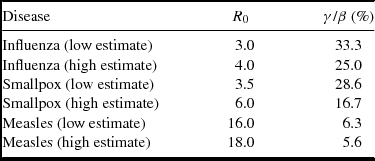
Table 1 presents estimates of R ₀ (pronounced “R-zero”) for several diseases, along with their reciprocals γ/β for a population normalized to 1. Thus, for example, smallpox cannot switch from an isolated outbreak to an epidemic (in a deterministic model) unless the susceptible portion of the population exceeds about 29%. After an epidemic begins, the number of susceptible individuals eventually declines to below γ/β, and the epidemic dies out. As disease-induced immunity wanes, or as recovered individuals die from other causes and are replaced through new births, the fraction of susceptible individuals creeps back up until an epidemic again occurs. Such long-term patterns are addressed in more complex SIR models than the one presented here.

Table 1.

Estimates of R ₀ for Selected Diseases.

Note: R ₀ = average number of secondary cases arising from an average primary case in an entirely susceptible population; γ/β = 1/R ₀, the minimum initial fraction of a population (here expressed as a percentage) that must be susceptible to a disease for an infection to spread.

Source: Keeling and Rohani Reference Keeling and Rohani2008:Table 2.1.

Stochastic Threshold Effect Based on Population Size

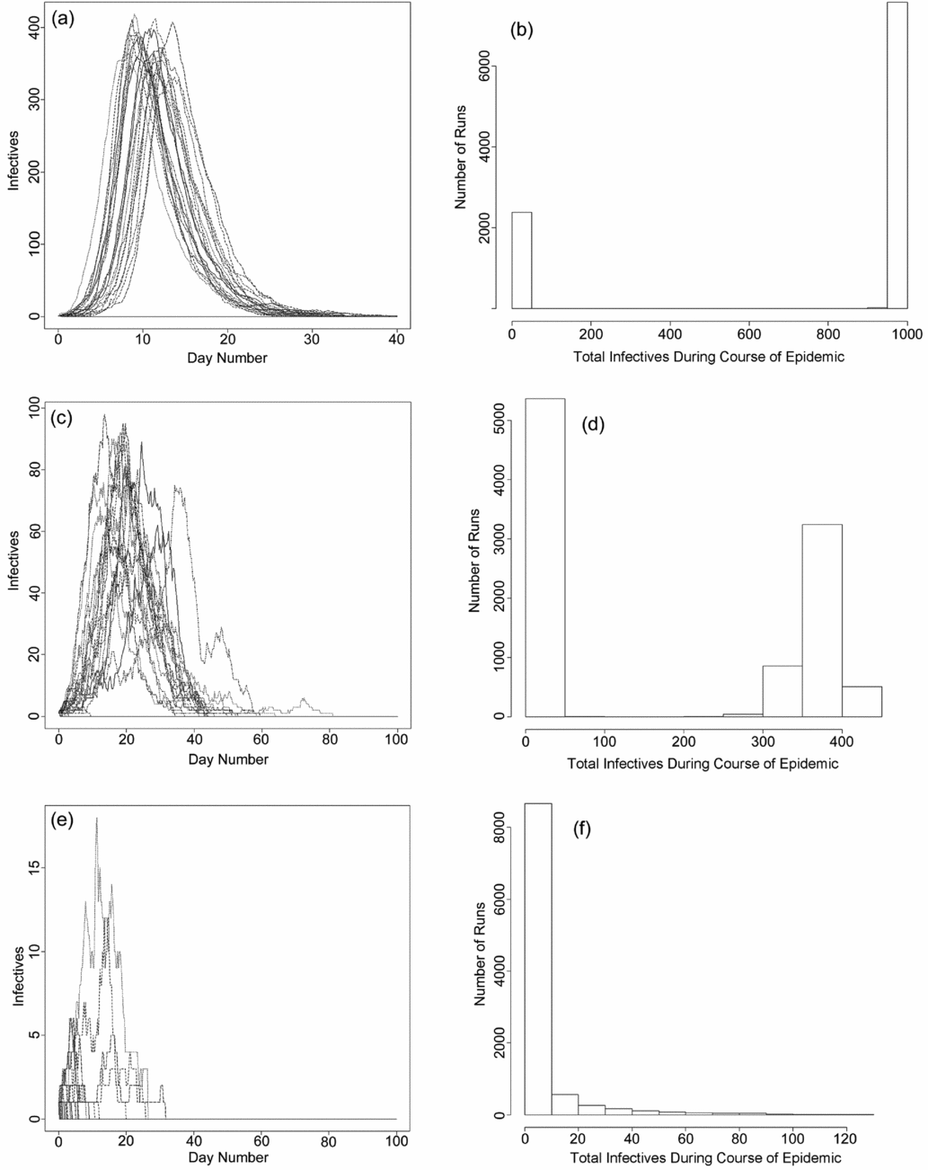
Program 1 (Phillips et al. Reference Phillips, Wearing and Clark2017) provides the code for a simple SIR model of disease among 1,000 susceptibles (a common village size for the Southwest/Northwest after AD 1300). The community also includes one infective (to introduce the disease) and no recovereds. The model assumes that infection and recovery are stochastic processes (as opposed to the deterministic approach indicated by Equation 1), that R ₀ = 3.5, and that, on average, infectives recover after three days. Figure 2a shows 30 runs of the model, yielding fairly similar results: about one-third of the village consists of infectives at the peak of an epidemic.Footnote ²

Figure 2.

Simple, stochastic Susceptible-Infectious-Recovered (SIR) model of epidemics in communities of 1,000, 500, and 250 initial susceptibles. (a) Based on 30 runs of the model, one-third of the community of 1,000 is infectious at the epidemic's peak. Each line represents one run of the model; the small number of runs allows readers to see individual runs. (b) Based on 10,000 runs, in most cases the epidemic sweeps through the village. (c) Based on 30 runs, fewer than one in five persons in a community of 500 are sick at the peak of an epidemic. (d) Based on 10,000 runs, communities of 500 escape the epidemic far more often than communities of 1,000. (e) Based on 30 runs, during epidemics fewer than one in 10 individuals in a community of 250 are sick at the peak of the epidemic. (f) Based on 10,000 runs, epidemic “fizzles” are the usual outcome.

The data for 10,000 runs indicate that, on average, 74.0% of the initial susceptibles fall ill across all runs. In most cases, 90.0% or more of the population has been infectious by the end of the epidemic (Figure 2b). This outcome reflects a situation where initially no one is immune to the disease—corresponding to, say, the arrival of smallpox in an area never exposed to it. Even so, due to the chance nature of transmission, in 23.9% of the runs the epidemic infected no more than 5.0% of the population (in 18.7% of the runs, no one was newly infected). Theory based on branching processes has shown that if a single infective is introduced into a fully susceptible population, the probability of an epidemic is about 1 − 1/R ₀, about 71.4% in this case (see Whittle Reference Whittle1955).

Halving the number of initial susceptibles, S(0), to 500 and lengthening the runs to 100 days, while leaving other parameters and initial states unchanged, increases the time required for epidemics to die out, and the epidemic “spike” becomes less consistent from run to run. Now, at the peak of an epidemic, one-fifth or less of the village consists of infectives (Figure 2c). For 10,000 runs at S(0) = 500, an average of 34.7% of initial susceptibles become infectives over the course of the runs. Moreover, 53.4% of the runs resulted in fewer than 5.0% of the initial susceptibles becoming infectives, and 33.7% of the runs resulted in no new infections (Figure 2d).

Reducing S(0) to 250 (about the size of many larger villages before AD 1200) produces epidemics that usually peak with less than 10.0% of a village being infectives (Figure 2e). For 10,000 runs over 100 days, an average of 0.6% of the initial susceptibles became ill by the end of the runs. Also, 88.2% of the runs resulted in an epidemic that affected less than 5.0% of the total population, and 51.2% of the runs resulted in no new infectives. These dramatic reductions were accompanied by a qualitative change in the distribution of total infectives (Figure 2f). Instead of a distribution split between the “fizzled-out” and pervasive epidemics, we have a rapid tailing off of the size of only minor outbreaks.

The values of S(0) used in these runs are relevant to regional demography. If we assume that every village is half susceptibles and half recovereds (the latter due to prior epidemics), villages at the upper end of the Southwest/Northwest size range could easily contain 500 to 1,000 susceptibles, while earlier settlements would have contained 100 or fewer susceptibles. In the large villages, stochastic effects would allow villages to “dodge the bullet” on rare occasions, but most of the time epidemics, once introduced, would sweep through the village. In contrast, we can expect small villages to have escaped epidemics on a regular basis. The pathogen need not change; household-level human behavior need not change. EIDs could be triggered by aggregation alone.

A Zero-Order Approximation Using an SIS Model

In a Susceptible-Infectious-Susceptible model, one does not gain immunity from prior infection; recovered individuals cycle back into the susceptible pool. Dysentery is a good example. The simplest SIS model corresponds to Figure 1b, where the entire population consists of either susceptibles or infectives (N = S + I). The system of differential equations is even simpler than for the SIR model:

(3a) $$\begin{equation} \frac{{dS}}{{dt}} = - \beta SI + \gamma I\\ \end{equation}$$

(3b) $$\begin{equation} \frac{{dI}}{{dt}} = \beta SI - \gamma I \end{equation}$$

(4) $$\begin{eqnarray} \frac{{dI}}{{dt}} &=& \beta (1 - I)I - \gamma I = \beta I\left( {1 - I - \frac{\gamma }{\beta }} \right)\nonumber\\ &=& \beta I\left( {1 - I - \frac{1}{{{R_0}}}} \right) \end{eqnarray}$$

We can find values of I at which the number of infectives is not changing with time by setting the rate of change, dI/dt, to zero. Because all the parameters are positive,

(5) $$\begin{eqnarray} \frac{{dI}}{{dt}} &=& \beta I\left( {1 - I - \frac{1}{{{R_0}}}} \right)\nonumber\\ &=& 0 \Rightarrow I = 0,\,\,\,1 - I - \frac{1}{{{R_0}}} = 0 \end{eqnarray}$$

The first option (I _endemic = 0) means that no one is infectious. The second option can be rewritten as

(6) $$\begin{equation} {I_{endemic}} = 1 - \frac{1}{{{R_0}}} \end{equation}$$

Moreover, because S = 1 − I, we also know that

(7) $$\begin{equation} {S_{endemic}} = \frac{1}{{{R_0}}} \end{equation}$$

We now have two conditions under which the rate of infection does not change. Unlike in the simple SIR model where epidemics eventually die out, if R ₀ > 1, the simple SIS model (with infection present) trends to an equilibrium state of S = S _endemic, I = I _endemic, where the disease persists indefinitely (Keeling and Rohani Reference Keeling and Rohani2008:39).

Stochastic Threshold Effect Due to Population Size

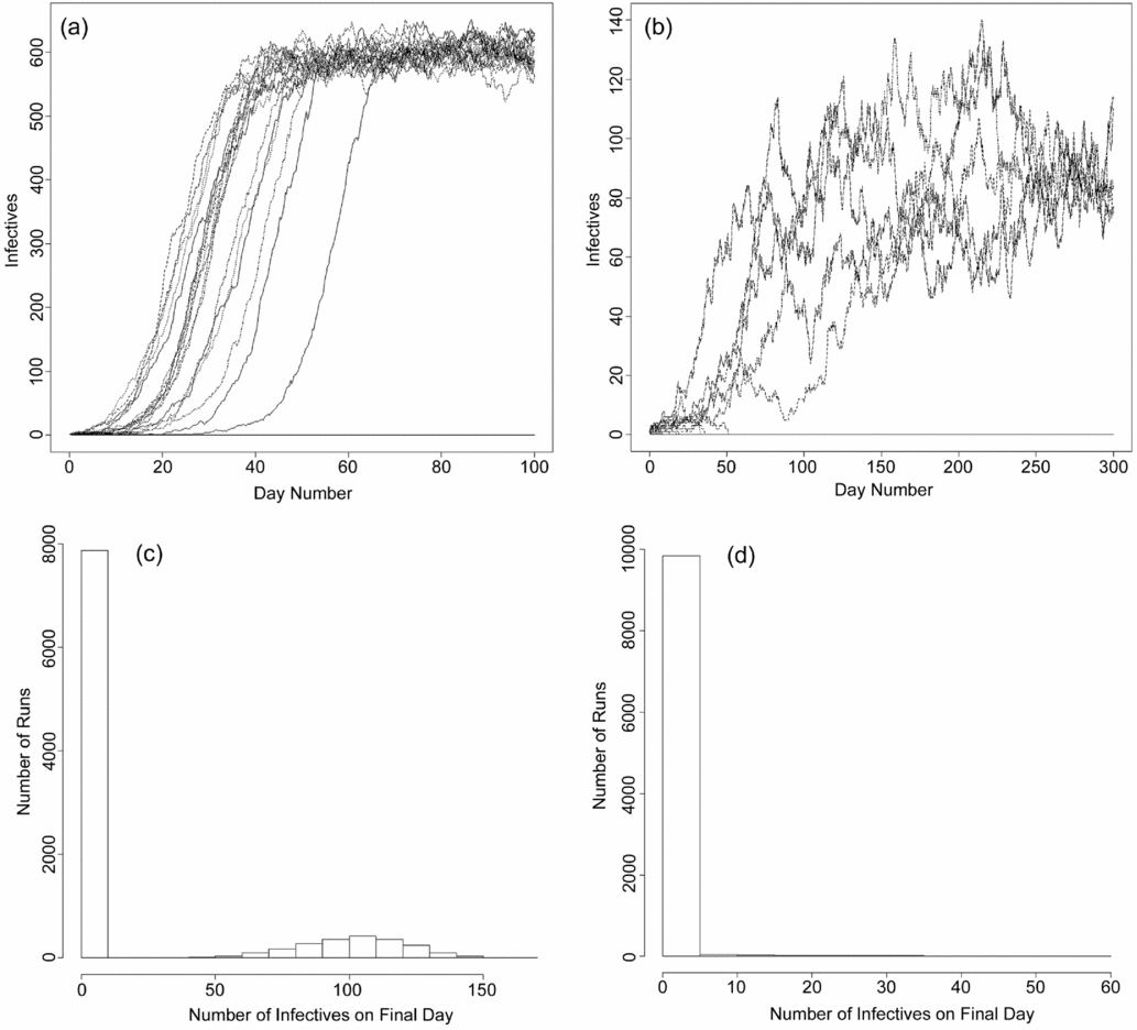
The code for a stochastic SIS model is included as Program 2 (Phillips et al. Reference Phillips, Wearing and Clark2017). Again, the population is 1,000. In this case the disease is less infectious (R ₀ = 2.5), but the mean duration of infection is seven days.Footnote ³ As with the SIR model, both infection and recovery are simulated as stochastic processes. For S(0) = 1,000, in most runs the disease tends to become endemic with infectives making up roughly 60% of the population (Figure 3a). However, 38.9% of 10,000 runs result in disease-free populations.

Figure 3.

Simple, stochastic Susceptible-Infectious-Susceptible (SIS) model of epidemics in communities of 1,000, 500, and 400 initial susceptibles. (a) Results of 30 runs for a community of 1,000 initial susceptibles. When infection spread it stabilized at about 60% of the population. (b) For S(0) = 500, when the disease took hold, only about 20% of the population was affected. (c) In most of the 10,000 runs for S(0) = 500, the disease does not take hold. (d) In 10,000 runs for S(0) = 400, the disease almost always fails to become endemic, and in the exceptions, the level of infection is very low.

For S(0) = 500, the trend through time is less consistent (Figure 3b). For 10,000 runs, 78.7% of the population are disease-free after 300 days (Figure 3c). In 10,000 runs with S(0) lowered to 400 (Figure 3d), 98.9% of the population are disease-free after 300 days. In 0.6% of the runs the disease is still present and infecting more than 5.0% of the population.

Again, we see the effect of aggregation. When the modeled populations are small, the pathogen either does not take hold or affects a modest fraction of the population. When the modeled populations grow, the same pathogen routinely becomes embedded in communities, often infecting a large proportion of each population.

A First-Order Approximation SIR Model with Demography

In the next two sections, slightly more complicated models step away from purely illustrative examples toward regional prehistoric reality. In the first model we examine the regional demographic trends for the SWSN study area: an estimated increase from 100,000 to 160,000 between AD 1200 and 1325, followed by a decline to 75,000 by AD 1550. We provide this model in response to a specific question, posed to help us build our argument: If the study area was sufficiently connected to be treated as a single population, for an SIR-type disease, what R ₀ would account for the documented decline? Because of the large population size, we used a frequency-dependent model. We sought only the expected (average) outcome, so for the first time we simulated a deterministic model. The corresponding differential equations are

(8a) $$\begin{equation} \frac{{dS}}{{dt}} = (\mu + \delta )N - \beta S\frac{I}{N} - \mu S\\ \end{equation}$$

(8b) $$\begin{equation} \frac{{dI}}{{dt}} = \beta S\frac{I}{N} - (\gamma + \mu + \nu )I\\ \end{equation}$$

(8c) $$\begin{equation} \frac{{dR}}{{dt}} = \gamma I - \mu R, \end{equation}$$

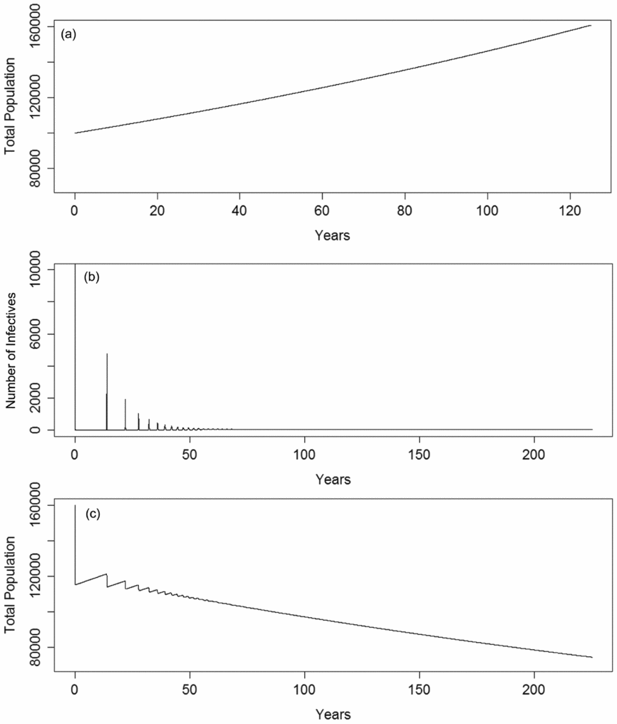
The computer model (Program 3; Phillips et al. Reference Phillips, Wearing and Clark2017) was run repeatedly, and the parameters β, γ, and ν were adjusted until a decline approximating the target was achieved. Figure 4a represents a run in the disease-free state where I(0) = 0. The initial population N(0) consisted of 100,000 susceptibles and no recovered and immune individuals. This run merely confirms that absent the added mortality from epidemic disease, the total population increased as expected. In Figure 4b the initial population N(0) included 160,000 susceptibles, no recovered and immune, and one infectious individual. The initial epidemic shrank the population by 28%, at which point the lowered proportion of susceptibles caused the epidemic to die out. Population regrowth increased the ratio of susceptibles to recovereds, and the disease rebounded. The cycle repeated, while overall population declined (Figure 4c).

Figure 4.

Results of two runs of the Susceptible-Infectious-Recovered (SIR) model with demography. (a) Absent the disease, over 125 years the population increases from 100,000 to 160,801. (b) After the initial outbreak, smaller outbreaks occur on a periodic basis. (c) During the 225 years after the initial outbreak, the population declines from 160,001 to 74,489.

The parameters leading to these results include μ = 0.02 per year, corresponding to 20 births or deaths per 1,000 individuals per year, while δ = 0.0038 (the estimated average annual rate of increase between AD 1200 and 1325). Also, β = 1.35 per day, γ = 1/7 per day, and ν = 1/18 per day. For this model,

(9) $$\begin{equation} {R_0} = \frac{\beta }{{\gamma + \mu + \nu }} \approx 6.8, \end{equation}$$

a value slightly beyond high-end estimates for smallpox and well below low-end estimates for measles (Table 1). The final parameters further indicate that, on average, about 28% of infected individuals die—well within historical ranges for mortality due to infection (Centers for Disease Control and Prevention 2017; World Health Organization 2017a, 2017b).

If the computer model had required an R ₀ or other parameter outside the known ranges for infectious diseases, in order to achieve the observed drop in prehistoric population, we could immediately rule out infectious disease as a leading cause of the known decline (hence the utility of asking the question at the start of this section). The results point the other way, however: a single EID of the SIR type, with realistic parameters, could account for the entirety of the observed decline, if the region consisted of a single population. Nonetheless, we reject that tentative conclusion, for reasons explored in the next section.

A First-Order Approximation Based on a Southwest/Northwest Metapopulation

Suppose that an infection is present in Village 1 and that one resident of Village 2 visits one person in Village 1. Will the visitor contract the disease and take those germs back to Village 2?

The answer quickly takes shape as a probability. Suppose that when the visitor arrives in Village 1, one-quarter of the residents are infectious. Suppose also that close contact leads to infection half of the time. Even given that extremely high infection rate, the probability that the visitor will be infected in Village 1 is 0.25 × 0.5 = 0.125, or only one in eight! Of course, more between-village visits and increased contact during each visit will increase the odds of the disease spreading, but the implication is clear. When a population is distributed in two villages, part of that population is buffered from the spread of infectious disease.

In epidemiological parlance a system of interacting villages constitutes a metapopulation. In turn, those villages are subpopulations, “each of which has independent dynamics, together with limited interactions between the subpopulations” (Keeling and Rohani Reference Keeling and Rohani2008:237; see also Hanski and Gaggiotti Reference Hanski and Gaggiotti2004; Hanski and Gilpin Reference Hanski and Gilpin1991, Reference Hanski and Gilpin1997). In a deterministic model with two interacting subpopulations, an epidemic in one always spreads to the other. In contrast, in a stochastic model it is possible for the epidemic to fail to spread (Keeling and Rohani Reference Keeling and Rohani2008:239–240; Park et al. Reference Park, Gubbins and Gilligan2002).

The final simulations in this essay present a stochastic SIS model of disease spread among subpopulations (which we refer to as villages) constituting one metapopulation. The model includes the same SIS dynamic as before: in village i of m villages, susceptibles become infectives at a certain rate and recover and return to susceptible status at a different rate. In this case, however, an added factor F_i alters the rate at which susceptibles become infectives, based on the intensity of interaction among villages. The differential equations for the deterministic version of the model are

(10a) $$\begin{equation} \frac{{d{S_i}}}{{dt}} = - \beta {S_i}{I_i} - {F_i}{S_i} + \gamma {I_i}\\ \end{equation}$$

(10b) $$\begin{equation} \frac{{d{I_i}}}{{dt}} = \beta {S_i}{I_i} + {F_i}{S_i} - \gamma {I_i}, \end{equation}$$

(11) $$\begin{equation} {F_i} = \sum\nolimits_{j = 1}^m {f(} {I_j}),\,\,j \ne i, \end{equation}$$

where f is the rate at which susceptibles in village i contract the disease from infectives of a different village j.

The next task is to define f. To simplify this task we assume that only susceptibles travel between villages (infectives, being ill, stay home) and that patterns of visitation are uniform. Only day visits occur (so that the number of individuals in each village subpopulation is unaltered by visits). We let V equal the total number of visits to other villages by each healthy (susceptible) individual per day. Given m villages in all, the rate of visitation to each other village is V/(m − 1) visits per other village per susceptible person per day. Once a visitor reaches another village, consistent with a density-dependent approach we assume that the visitor is exposed to all infectives in the host village (by drinking from its contaminated water supply, for example). Thus, the rate of infection for visitors to village j is βI_j per visitor per day. Combining the rate of visitation per other village and the rate of infection for visitors, we have

(12) $$\begin{equation} f({I_j}) = \left( {\frac{{V\beta }}{{m - 1}}} \right){I_j} \end{equation}$$

per other village per person per day.

As in the zero-order SIS model, the target R ₀ = 2.5, and the mean time of infection is seven days. Program 4 (Phillips, Wearing, and Clark Reference Phillips, Wearing and Clark2017) allows users to select the number of villages, but we always used 10 per run. The total population of each village was set at 1,000. The simulations were for 180 days; the model was designed with an eye to gastrointestinal diseases spread by contaminated water, so we were interested in what might happen in a single warm season.

The computer model incorporates additional simplifying assumptions. The total population was static (no births or deaths), and each subpopulation consisted of the same number of initial susceptibles. The rates of infection and recovery were uniform across the subpopulations. The infection always began in the first subpopulation called up by the program; that village began with five infectives (a number that minimizes premature epidemic die-outs due to the stochastic nature of transmission).

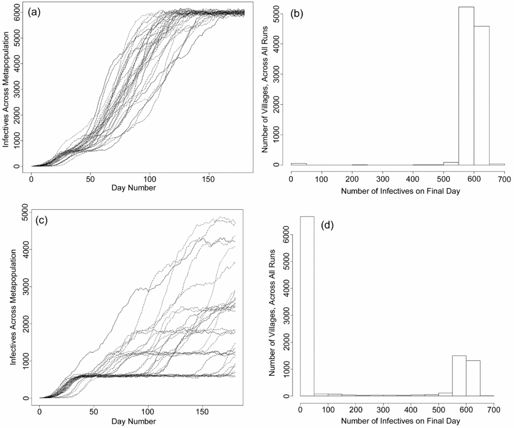
The simulations began with conditions chosen to ensure the spread of disease beyond the initially infected village; from there we reduced the amount of intervillage interaction and observed the effect. We began with one out of every 1,000 susceptible individuals (an average of one healthy person per village) visiting one other village each day (V = 0.001). A typical outcome is shown in Figure 5a, which is for 30 simulations. In run after run, the disease became endemic, actively infecting about 60% of the total population. In a series of 1,000 runs (Figure 5b), only 0.5% of the 10,000 modeled villages were uninfected after 180 days.

Figure 5.

Metapopulation model. All runs are for 10 villages (subpopulations), each with 1,000 initial susceptibles. (a) Results of 30 runs with V = 0.001 (one healthy person per village visits one other village each day). (b) Results of 1,000 runs with V = 0.001. On the final day of the run, the disease is actively affecting about 60% of the population of most villages. (c) Results of 30 runs with V = 0.0001 (one healthy person per village visits one other village every 10 days). (d) Results of 1,000 runs with V = 0.0001. On the final day of the run, most villages have few or no instances of the disease.

Reducing the frequency of visits to one every other day, per 1,000 susceptibles (V = 0.0005), results in a similar rate of endemic infection—but in 1,000 runs, 2.1% of the villages were uninfected after 180 days. For one visit every third day, 12.6% of the villages were uninfected. As the rate of visitation continued to drop, the number of uninfected villages steadily rose, and for the rest, after 180 days the rate of infection could be much less than the roughly 60% obtained earlier (Figure 5c–d).

The model indicates that if contact among subpopulations is low enough, in the short run disease is unlikely to spread throughout the metapopulation. The model also provides a first guess as to what “low enough” means. If, for example, we assume that on average one susceptible in 1,000 visited some other large village no more than once a month (V = 1/[9 × 10⁴]), in the short run an outbreak of an EID in the first village probably led to outbreaks in another village less than one in seven times. Admittedly, rates of visitation might have been high within clusters of villages, but between such clusters the rates of visitation may have been low enough to hinder the spread of disease.

Thus, we are not inclined to attribute the post–AD 1325 population decline to a single devastating pandemic similar to the Black Plague. Instead, the division of the Southwest/Northwest metapopulation into numerous subpopulations (villages and clusters of villages) should have fostered a slower, spottier infection process involving instances of local depopulation at different times. This outcome is, of course, the pattern of Southwest/Northwest demographic retrenchment as we now understand it.Footnote ⁴