1. Introduction
While India is still a developing country, carbon emission reductions in this country are needed in order to achieve ambitious global climate targets. Furthermore, realizing the relatively cheap abatement options in India helps to minimize global mitigation costs. In 2008, India ranked third in terms of absolute emissions after China and the US (if Europe is not taken as one entity) (World Bank, 2012). If rapid economic growth in India continues, emissions will rise further in the next decades unless climate policy counteracts this trend.
That India is still a developing country is reflected in its per capita income of only US$1,410 and 32.8 per cent of the population living on less than $PPP1.25 per day in 2010; per capita emissions of 1.5 t CO2 in 2008 were only one-third of the world average (World Bank, 2012). Not surprisingly, India's primary goal is to develop its economy and to reduce poverty. Yet in the Copenhagen Accord India pledged to reduce emissions per unit of GDP by 20 per cent to 25 per cent in 2020 relative to 2005. This reduction is voluntary and not legally binding (GOI, 2010a). Also, the targeted carbon intensity will possibly be reached even without new policy measures (Tavoni, Reference Tavoni2010; den Elzen et al., Reference den Elzen, Hof, Beltran, Grassi, Roelfsema, van Ruijven, van Vliet and van Vuuren2011; GOI, 2011). In addition, India also aims to implement more specific measures, stated, for example, in the Jawaharlal Nehru National Solar Mission, which targets 20 GW of solar electricity generation capacity by 2022 (GOI, 2010b).
Since mitigation efforts are costly and could conflict with the need for development, most global climate regime proposals include measures to at least partly compensate India for its mitigation costs. In particular, many emission trading proposals include surplus allowances that India can sell on an international carbon market (see, for example, van Ruijven et al., Reference van Ruijven, Weitzel, den Elzen, Hof, van Vuuren, Peterson and Narita2012). Assessments of the resulting costs for India are mostly carried out with the help of global models and indicate that India would either gain or face only little economic cost when joining an international climate regime (see van Ruijven et al., Reference van Ruijven, Weitzel, den Elzen, Hof, van Vuuren, Peterson and Narita2012, for an overview). Global models are useful because climate change is a global problem and only global models can analyze where abatement is most efficient. However, global models typically only represent the Indian economy in a highly aggregated way and furthermore often reduce the cost estimates for India to a single aggregate figure such as impact on GDP or welfare. There is, for example, no information on the distributional or regional impacts of climate policy.
Single-country models are used as well to assess the effects of climate policy measures for India. Many of these assessments are by energy system models focusing on the energy system (see, for example, Shukla and Dhar, Reference Shukla and Dhar2011). The models include various renewable energy technologies and a portfolio of specific policies such as urban planning and transport infrastructure (Shukla et al., Reference Shukla, Dhar and Mahapatra2008). Computable general equilibrium (CGE) models, in contrast, are able to include the economy-wide repercussions resulting from climate policy. Early applications include Fisher-Vanden et al. (Reference Fisher-Vanden, Shukla, Edmonds, Kim and Pitcher1997) who compare the cost of stabilizing Indian emissions unilaterally with the costs in a global regime, and Bussolo and O'Connor (Reference Bussolo and O'Connor2001) who assess the impacts of climate policy on four different Indian regions, taking into account the ancillary benefits of CO2 reduction. Besides disaggregated sub-regions, single-country CGE models can include different household types. This allows the determination of the distributional effects of climate change policies. Energy policies in India have a history of containing goals of social policies (e.g., subsidized fuels), albeit they are not always successful in fulfilling these goals (Rao, Reference Rao2012). Yet distributional impacts of any carbon abatement policy for India would be under scrutiny, especially with respect to its impact on the poorest.
The distributional effects of climate policies have been in focus before. Boccanfuso et al. (Reference Boccanfuso, Estache and Savard2011) present an overview of intra-country distributional impacts. The studies on industrialized countries are inconclusive as to whether the overall effects are regressive (e.g., Jorgenson et al., Reference Jorgenson, Slesnick, Wilcoxen, Goettle and Ho2011) or progressive (e.g., Oladosu and Rose, Reference Oladosu and Rose2007; Rausch et al., Reference Rausch, Metcalf, Reilly and Paltsev2010). There are fewer studies for developing countries. For Indonesia, Yusuf and Resosudarmo (Reference Yusuf and Resosudarmo2007) find carbon taxes to be progressive for rural households but neutral to progressive for urban households. For China, Boyce et al. (Reference Boyce, Riddle and Brenner2005) find that carbon taxes would be progressive, while according to Liang and Wei (Reference Liang and Wei2012) they would widen the rural–urban income gap without transfers to rural households. For the Philippines, Corong (Reference Corong2008) finds that higher skilled workers have higher welfare gains when carbon tax revenues are used to reduce income taxes. In general, the progressivity of a carbon tax depends on the design of revenue recycling, the differing carbon intensity of consumption, and changing demand for factor endowments of different households. For India, two papers analyze the impact of climate policy on poverty. Murthy et al. (Reference Murthy, Panda and Parikh2007) find that a decrease in per capita income leads to an increase in poverty. Ojha (Reference Ojha2009) finds an increase of poverty which cannot be eliminated but significantly reduced if tax revenue is transferred to poor household groups.
In single-country CGE models, India is usually modeled as a small open economy; that is, it is implicitly assumed that national climate policy is carried out in the absence of climate policy abroad and has no effect on world markets. Global models, however, are able to simulate international carbon markets and repercussions on international energy markets. In this paper we want to bring together both types of models to overcome the shortcomings of the existing analyses which are either very aggregated or ignore international repercussions. We do so by soft-linking the multi-region CGE model DART to a one-country CGE model for India, in order to take advantage of the specific capabilities of both types of models. In particular, we analyze on the one hand the distribution and allocation effects of international climate policy regimes for India in more detail, while on the other hand we account for two important implications of a global regime, namely the impact of international transfer payments and price repercussions on international markets.
As mentioned above, financial transfers are seen as a means to compensate for mitigation costs. In some cases these financial flows can be substantial and can influence exchange rates and thus the competitiveness of countries. This issue was first debated between Keynes and Ohlin in 1929, but has also been applied to climate change regimes (McKibbin et al., Reference McKibbin, Shackleton and Wilcoxen1999a, Reference McKibbin, Ross and Shackleton1999b). The multi-regional, perfect foresight model of McKibbin et al. includes a rather sophisticated representation of international financial flows based on returns to investment and trade in carbon permits. While there is no explicit modeling of exchange rates in DART, the national model captures some of the exchange rate movements.
Concerning price repercussions on international markets, ambitious climate policy has the effect that carbon intensive products become (relatively) more expensive, and that fossil fuels are demanded less. Countries that are net importers of fossil fuels – such as India – can thus benefit from lower energy prices (net of carbon prices) through improved terms of trade. CGE models are able to capture these repercussions as the interplay between markets is taken into account. This fuel price effect is acknowledged in global models (e.g., Böhringer and Rutherford, Reference Böhringer and Rutherford2002) but to our knowledge not in any national model study for India. We thus pass on variations in international fuel prices from the global model to the national model so that the changes in the terms of trade are accounted for. The national model then shows which types of agents in the economy profit from this effect.
Since a considerable share of the Indian population still lives below the poverty line, the impact on poor household groups is of particular importance. We thus focus on the distributional impacts of climate policy and analyze how carbon pricing, (international) transfer payments and international price repercussions affect different household groups. Compared to earlier studies mentioned above, we extend the simulation horizon to 2050 and incorporate current climate policy (Copenhagen pledges) into the analysis. By using harmonized models, there is greater consistency when feeding global data such as prices for CO2 or energy into the national model. With such a soft-link of the two models we aim in particular to shed light on the following research questions: how do insights from a national model change when taking into account the fact that the rest of the world is also engaging in climate policy and causing changes on international markets? How robust are the results from the national model when changing the outside world? How does the more detailed analysis of the national model compare to the international broad picture?
The paper is structured as follows. Sections 2 and 3 describe the models and the policy scenarios, respectively. Focusing on the distributive effects for different household types as mentioned above, section 4 presents and discusses the results. Section 5 concludes.
2. Model description
In this study, two CGE models are used. While DART is a multi-regional model of the entire world economy, IEG-CGE is a national model of the Indian economy. Both models are multi-sectoral, recursive-dynamic models solving for a sequence of static one-period equilibria for future time periods. The time horizon of this study is 2050.
DART (Klepper et al., Reference Klepper, Peterson and Springer2003; Weitzel et al., Reference Weitzel, Hübler and Peterson2012a) is based on the GTAP 7 data set (Narayanan and Walmsley, Reference Narayanan and Walmsley2008) with the base year 2004, aggregated to 12 sectors and 13 regions including India (see Weitzel et al., Reference Weitzel, Ghosh, Peterson and Pradhan2012b). Based on bottom-up information, the electricity sector is split into conventional generation and new generation technologies from four renewable sources (wind, solar, biomass and hydro); additionally electricity generation with carbon capture and storage (CCS) from gas and coal is introduced as a latent technology (Weitzel, Reference Weitzel2010). Electricity from different generation technologies is assumed to be a perfect substitute; each technology has a convex cost function and exhibits learning.
IEG-CGE (Pradhan and Ghosh, Reference Pradhan and Ghosh2012a, Reference Pradhan and Ghosh2012b) consists of 18 sectors rather similar to the DART sectors (see Weitzel et al., Reference Weitzel, Ghosh, Peterson and Pradhan2012b). The main data source is a social accounting matrix (SAM) for India (for 2003–2004) developed by Ojha (Reference Ojha, Pal, Pohit and Roy2009) that decomposes the electricity sector into hydro, nuclear and nonhydro-electricity. For this study the nonhydro sector was further disaggregated into thermal and wind/solar electricity. In addition, a sector that uses CCS technology (coal) to produce electricity was created. It is less efficient than the thermal electricity sector and produces emission-free coal-based electricity.
Producer behavior in both models is derived from cost minimization for a given output or equivalent profit maximization. All industry sectors are assumed to operate in perfectly competitive markets and at constant returns to scale. A multi-level nested separable constant elasticity of substitution (CES) function describes the technological possibilities (Weitzel et al., Reference Weitzel, Ghosh, Peterson and Pradhan2012b describe the CES nesting). Primary factors include labor and capital and in DART also land. Factor markets are assumed to be perfectly competitive and there is full employment of all factors which are sectorally mobile, but in DART regionally immobile.
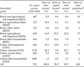
Households maximize utility subject to income and prices. Household demand is modeled through the Linear Expenditure System (LES) that first satisfies basic needs. The remaining consumption good is a composite of an energy and a non-energy aggregate. Household income comprises factor income and transfers from the government and the rest of the world. Households also save a fixed part of their incomes and pay taxes to the government. In DART, there is one representative agent (RA) in each region; households in IEG-CGE are classified into five rural and four urban categories (see table 1).Footnote 1 Two rural and one urban household types with low per capita income are characterized by a lack of capital income and can be considered as poor. Richer households have a higher expenditure share for services; the share of energy expenditure is slightly higher for poor households (see the online appendix available at http://journals.cambridge.org/EDE). This difference in preferences is captured in the calibration of the LES. When households become richer, the share of services in their expenditure increases.
Economic indicators for the different household groups in the base year (2004)

Notes: Calculations from SAM. Households marked with an asterisk are considered as poor in this study. a Household factor income shares based on Pradhan and Roy (Reference Pradhan and Roy2003). b Population shares from Sundaram and Tendulkar (Reference Sundaram and Tendulkar2003). c Remaining capital income goes to public and private enterprises, government, and rest of the world. Exchange rate assumed to be 44 Rupees per US dollar.
Both models follow an investment-driven closure, i.e., aggregate investment is fixed. In DART, only households save at a fixed exogenous rate. In IEG-CGE, aggregate savings is the sum of household, government, corporate and foreign savings and adjusts to satisfy the saving–investment balance. Foreign savings are assumed to be fixed while the real exchange rate is flexible. Government expenditure for consumption of goods and services, transfers to households and enterprises is fixed. Government savings are determined residually.
In DART, all regions are linked by the bidirectional trade flows of all commodities except the investment good and in both models domestic and foreign commodities are imperfect (Armington) substitutes. They are also distinguished by the country of origin in DART. There is no direct balance of trade constraint; only at the global level does trade have to be balanced.
In DART, the major exogenous, regionally different driving factors of the model dynamics are growth in population, labor productivity and human capital. Rather similarly, IEG-CGE assumes exogenous growth rates for total factor productivity (TFP), the labor force, government consumption expenditure and aggregate investment. In both models, capital accumulation is driven by exogenous depreciation and savings rates. To capture future increases in energy efficiency, we assume an autonomous energy efficiency improvement of 1 per cent per year (0.1 per cent in the electricity sector) in DART and 1.5 per cent in IEG-CGE. In both models GDP growth is calibrated by adjusting factor productivities. In DART, global CO2 emissions are calibrated by adjusting the elasticities of fossil fuel supply. In IEG-CGE, exogenous drivers for CO2 emissions are fossil fuels prices and energy efficiency improvement.
3. Scenarios
3.1. Baseline scenario [BAU]
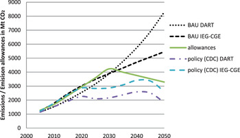
The models were harmonized with respect to GDP and population (i.e., labor force) projections. The GDP path follows the reference scenario of the OECD Environmental Outlook (OECD, 2012). Population projections are based on the medium variant of UN World Population Prospects (UNDESA, 2011). Global population is projected to increase to 9.5 billion people in 2050, with 1.6 billion in India. Energy use and therefore CO2 emissions differ between the models (see Johansson et al., in press, for a detailed comparison on energy use). In DART, global emissions reach 54 Gt CO2, with India contributing 8.3 Gt. In IEG-CGE, baseline emissions are only 5.5 Gt in 2050. As figure 1 shows, emissions in IEG-CGE are growing faster than in DART in the near future, while emissions in DART are higher after 2030. Both models project little change in the carbon intensity in the baseline; a higher improvement in the energy intensity in IEG-CGE explains the difference in CO2 emissions.
Indian emissions under the BAU and policy scenarios in DART and IEG-CGE

3.2. Climate policy scenarios
It is not possible to implement a dynamically efficient climate policy in a recursive-dynamic model. We therefore adopt a ‘standards and prices approach’ (Baumol and Oates, Reference Baumol and Oates1971), i.e., take an exogenous emission path and determine the minimal cost to achieve this path. The emission path incorporates the Copenhagen pledges until 2020. After 2020, it is derived from intertemporal optimization with the target of avoiding a global temperature rise of more than two degrees compared to pre-industrial times with 50 per cent probability (see Johansson et al., in press, for a discussion of the pathway). In the basic climate policy scenario, global energy-related emissions peak in 2020 at a level of 34 Gt CO2 and are subsequently reduced to 17.6 Gt in 2050. Compared to baseline emissions, this is a reduction of 67 per cent, or 17 per cent below 1990 emissions. Global harmonization of marginal abatement cost is reached via global emission trading. We hold global emissions constant in all policy scenarios; that is, there are no efficiency gains or losses from changing the temporal emission dynamics dimension between scenarios in order to avoid confounding welfare effects.
To derive a first best policy outcome, a forward-looking model would be necessary. Babiker et al. (Reference Babiker, Gurgel, Paltsev and Reilly2009) compare a recursive-dynamic to a forward-looking model and conclude that while forward-looking dynamics have preferable theoretic properties, the simulation differences in the energy sector were relatively small. Macroeconomic costs were lower in the forward-looking model because of consumption smoothing. However, the forward-looking dynamics forced the modelers to simplify the technological detail to achieve computational feasibility. Our aim is not to find the cost minimal pathway for emission reductions, but we are interested in the differences between several scenarios that all incorporate the Copenhagen pledges. These pledges are not dynamically efficient because they were set politically. For our purpose a recursive-dynamic model is therefore justified.
For India, CO2 emission reductions in the policy scenarios are determined endogenously. In DART, they are the result of equalizing marginal abatement costs globally. In the national model, CO2 prices are taken from DART and imposed as a domestic carbon tax. For the simplest scenario, this is the only model link. Fisher-Vanden et al. (Reference Fisher-Vanden, Shukla, Edmonds, Kim and Pitcher1997) and Shukla et al. (Reference Shukla, Dhar and Mahapatra2008) also use this methodology; however, our study is potentially more consistent because the global and the national model are harmonized to some degree. Due to differences in abatement potential and costs in the two models, the policy pathways turn out to be somewhat different. Both models stay near the baseline close to 2020, followed by a longer stabilizing period. After 2020, effort has to be increased in order to reach the overall reduction target. This leads to a higher global CO2 price which also slows Indian CO2 emissions. Emissions in both models peak in the 2040s and decline towards 2050. Abatement potential becomes increasingly scarce, especially after 2040, which leads to high CO2 prices of 441 US$2004 in 2050, compared to 146 US$2004 in 2040 (see table A1 in the online appendix or Johansson et al., in press, for the entire path). Compared to the baseline, both models show improvement in both carbon and energy intensity.
3.2.1. Revenue allocation
How revenues from domestic carbon taxes are used is important because they can potentially bring about a double dividend.Footnote 2 There is also a discussion of an additional third dividend in terms of reduced poverty (see, for example, van Heerden et al., Reference van Heerden, Gerlagh, Blignaut, Horridge, Hess, Mabugu and Mabugu2006, who also briefly review the relevant literature). We distinguish between three different uses of revenue:
-
• [all] Revenues are transferred to all households groups based on their population share. This is closest to the assumption of the DART model where one RA receives all revenues. This scenario is equivalent to an equal per capita allocation of emission rights for all Indian households.
-
• [poor] Revenues are transferred only to the poor household groups based on the respective population shares of RH2, RH3 and UH3.
-
• [gov] Instead of making lump-sum payments to households, the revenues are used for government investments. This leads to crowding-out and lower savings from other agents.
3.2.2. International transfers
To account for the different development status of countries, many regime proposals include a transfer of funds. We model a common-but-differentiated-convergence (CDC) regime (Höhne et al., Reference Höhne, den Elzen and Weiss2006), which allows emissions of developing countries to peak later than emissions of developed countries. We assume that all countries first fulfill their (high) Copenhagen pledges and subsequently Annex I countries converge to 1.7 t CO2 per capita in 2040, while other countries start their 30-year convergence period between 2020 and 2035 (see Johansson et al., in press, for the detailed assumptions). In this regime, India enters in 2030 and converges in 2060. India's allowances peak at 4.23 Gt in 2030, and amount to 3.29 Gt in 2050 (see also figure 1).
Under the CDC regime, India sells emission allowances on the international carbon market. In the Indian model, international carbon trade is not modeled directly. In addition to the domestic carbon tax (with the carbon prices from DART), capital flows from international carbon trade are calculated from the difference of (exogenous) allowances with (endogenous) actual emissions in the Indian model, multiplied by the (exogenous) carbon price.Footnote 3 The revenues from international carbon trading are allocated in the same way as the revenues from domestic carbon tax (see section 3.2.1). The magnitude of financial flows rises over time, due to the rising CO2 price. When the revenue is expressed as a share of GDP, it reaches 3.2 per cent in DART and 2.1 per cent in IEG-CGE in 2030, and 4.7 per cent in DART and 2.2 per cent in IEG-CGE in 2050, respectively. Revenue in percentage of GDP is lower in 2040 (2.0 per cent in DART and 0.6 per cent in IEG-CGE) due to lower surplus emissions in that year (see also online appendix). Generally, the DART model projects a higher amount of permits sold on the international carbon market than IEG-CGE; hence capital flows are higher. However, each model is internally consistent and the price of carbon is equal in both models.
Because DART is based on data in real values, there is no exchange rate. Allowances are allocated to the RA in the respective regions. Changing the allocation of allowances implies a transfer of income from one region to another. Compared to a scenario where the globally efficient reductions are reached via a harmonized global carbon tax so that there are no financial transfers, the RA in India enjoys a larger endowment of allowances in the CDC scenario which increases national income. This leads in turn to demand changes in India, which are partly fulfilled by domestic production and partly by imports. This means that consumption as well as relative prices rise and therefore Indian trade is affected in DART, not because there is a change in the exchange rate but through the income transfer as such. In IEG-CGE, in all scenarios with capital inflows, demand is increased for the same reasons as explained above. In addition, in IEG-CGE the exchange rate decreases, i.e., the rupee appreciates, as a result of the capital inflow. This leads to higher imports and lower exports.
In order to assess how insights from a national model change when taking into account the fact that the rest of the world is also engaging in climate policy and causing changes on international markets, we run a set of scenarios with IEG-CGE using carbon prices from DART. The scenarios differ in the dimension of the (real) amount of transfers and the usage of carbon revenue. The (real) amount of capital inflow is varied both by different modeling and policy assumptions focusing on commonly made proposals:
-
• [noTr] No international transfers are assumed. This scenario is similar to a globally harmonized carbon tax regime with no compensation payments. The tax rate for the domestic CO2 price in India is taken from the DART model.
-
• [Tr-Rup] Transfers take place and are based on the allowances that India is able to sell on the international carbon market under the CDC regime. Here we denominate the transfers in rupees, i.e., fix the exchange rate for the carbon price at the base year. This excludes the effect of the Indian appreciation; that is, the exchange rate changes are as in the [noTr] scenario in which the exchange rate reacts only to a change in the demand and production structure.
-
• [Tr-$] Recognizing that transfer payments will not be carried out in rupees and can potentially shock the exchange rate, we denominate the carbon price in US$. Due to the resulting appreciation, real transfer payments are smaller than in [Tr-Rup].
3.2.3. Repercussions in international markets
IEG-CGE is a small open economy model, with the underlying assumption that India and the rest of the world do not affect each other through price changes. In the climate policy scenario, there are hence no international repercussions in IEG-CGE. In DART, the main repercussions are twofold: on the one hand, climate policy is carried out globally; hence global world market prices (especially for fossil fuels) change because of the carbon price and a reduced demand for fossil fuels. On the other hand, the Indian economy is affected by the climate policy which is reflected in changing demand patterns, leading to different import and export prices for other goods as well. The latter effect is smaller in terms of price changes and is thus neglected in this study.
In terms of modeling, we pass on relative price changes due to international climate policy from DART to IEG-CGE for each simulation year. In DART, export prices for India result from a transformation function where producers produce for the domestic and the world market. For imports, a nested Armington function is used. In a first stage, a composite of goods from different regions is aggregated, which in a second step is combined with domestic varieties. We pass on prices of this first step composite to IEG-CGE (relative to an Indian price index, which is used as the numéraire in the Indian model). Again, we harmonize prices; quantities in trade volumes are not harmonized and can differ between models.
We differentiate between three scenarios with different extents of passing on price information from DART:
-
• [P-exo] The same exogenous world market prices are assumed for IEG-CGE both in the baseline and the policy scenario. This scenario is standard for most single-country analyses, but fails to account for repercussions on international markets.
-
• [P-fuel] Relative changes in fossil fuel world market prices due to climate policy are passed on from the DART model, i.e., are different between the baseline and policy scenario.
-
• [P-all] Relative world market price changes for all sectors due to climate policy are passed on from the DART model. This also accounts for interconnections through intermediate markets. Since sectoral aggregation differs slightly between the two models, the price changes were mapped to different sectors where appropriate.
With the help of these scenarios we can analyze the distributional impact of international price repercussions, i.e., the impact on different household groups. In combination with the variations concerning capital inflows, we can also derive interactions between price effects and transfer payments.
4. Simulation results
Soft-linking DART to IEG-CGE generally affects all model outcomes of IEG-CGE. For example, CO2 emissions and production of energy-intensive goods rise when lower fossil fuel prices resulting from international climate policy are passed on from DART to CGE-IEG. All sectoral production as well as export and import levels react to the relative changes in input prices. While we discuss some of the relevant reactions in IEG-CGE, as for example the changes in sectoral production levels resulting from different assumptions about the allocation of transfers, our focus is on the welfare and income gap changes for the different household groups in order to assess how different groups are affected by international climate policy. All results are taken from the national CGE model if not stated otherwise. We also briefly discuss the overall welfare changes in IEG-CGE and DART.
4.1. Effects of revenue allocation
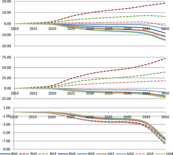
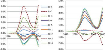
The welfare impacts of our basic climate policy scenario implemented via a (domestic) carbon tax are comparable to previous estimations of single-country CGE models. In our first analysis, we vary the recipients of the tax revenue and there are no international transfers. The resulting welfare losses for different household types relative to the BAU scenario without climate policy are shown in figure 2.Footnote 4 Not surprisingly, the decision of how to use the revenue of a carbon tax is crucial for how the households' welfare is affected. The top part of figure 2 shows welfare losses for a domestic carbon tax with lump-sum payments of the tax revenue to [all] households which is equivalent to equal per capita emission rights. In this case, poor households as defined above (RH2, RH3 and UH3) can gain substantially. Despite the fact that tax revenue remains below 5 per cent of GDP in 2050, gains for the ‘poor’ RH2 group can reach almost 20 per cent. Per capita transfer payments are higher for poorer households relative to their consumption expenditure. Furthermore, the LES consumption framework assumes a higher share of subsistence consumption for poorer households. Equal per capita gains thus lead to higher welfare changes for poor households. On the contrary, richer households are negatively affected. The overall more pronounced effects towards 2050 are due to the high CO2 tax and the lack of abatement possibilities in the models (see also Johansson et al., in press). In this scenario per capita income of poor households reaches 63 per cent of rich households' per capita income in 2050 (compared to only 40 per cent in 2005 or 54 per cent in the [BAU] scenario in 2050). The reduction of the income gap occurs within groups; that is, poor urban (rural) households reduce the gap to rich urban (rural) households. This holds especially for poor rural households who are the households with the lowest per capita income. However, the relative income difference between urban and rural households increases over time both in the [BAU] and the policy scenario.
Welfare impact (% Hicks EV) for different households of domestic climate policy compared to the [BAU] scenario

If tax revenue is exclusively redistributed to the three [poor] household groups, these effects are reinforced. Compared to the other richer households groups, urban salaried households (UH2) are relatively unaffected. Welfare gains for poor rural households reach about 70 per cent in 2050. Towards the middle of the century, the per capita income of rural poor households reaches the level of other rural households.
The picture becomes rather different when government uses the tax revenue for investment by the government ([gov]). Now the effects are rather similar across household types, although poor households as well as UH2 are affected slightly more adversely than other household classes. The main explanation is that richer households reduce saving due to crowding-out and consume more instead. Furthermore, urban households spend a higher share of their income on less carbon intensive services for which the average carbon tax rate is lower. Because the savings rates of richer households are higher, GDP growth is slightly higher than in scenarios with more redistribution and thus the total (weighted) welfare losses are smallest in this scenario. In short, we find that while distributing tax revenue to households is progressive, using tax revenue for government investment is regressive. At the same time, using the revenue for investment decreases overall costs of climate policy.
4.2. Effects of international transfers
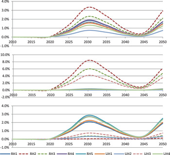
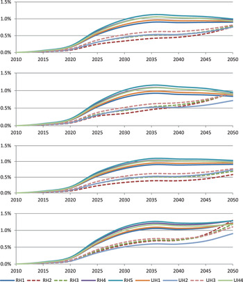
In a second step, we add international financial transfers to the model. This reflects an international regime (CDC) in which India is able to sell allowances on an international carbon market. To start with, we assume that the revenues from selling allowances are paid in lump-sum fashion to the households in addition to the tax payments and that transfers are in US$ ([Tr-$]). In figure 3 we isolate the effect of the additional revenue of international transfers; that is, we are analyzing welfare changes relative to the respective [noTr] scenario. The N-shape of the figures can be explained by the variation of revenues relative to GDP.
Welfare improvement of different households due to international financial transfers [Tr-$] relative to respective [noTr] scenarios under different allocation schemes

When the international transfer payments are distributed on a per capita basis to [all] households, poorer households gain more than richer households for the reason explained in section 4.1. The total welfare gains for poorer households from climate policy get stronger, while richer households can only partly offset their welfare losses from the scenario without international transfers. This effect is even stronger when transfer payments are restricted to [poor] household groups.
When transfer payments are used for government investments ([govt]), poor households profit less from the transfers than rich households, similar to the case when the tax revenue was used for government investments. Household groups with the highest gains from the capital inflow are in this case richer household types (except UH2). Transfers are able to fully offset the losses from CO2 emission reductions shown in figure 2 until the 2030s. Poorer households gain relatively little from the transfers under this scheme. The findings are broadly consistent with Ojha (Reference Ojha2009), who finds that poverty increases without targeted transfers of revenues to the poor. As carbon taxes and thus transfer payments in Ojha (Reference Ojha2009) are lower than in this study, the transfer schemes are not sufficient to fully compensate poor households.
Compared to figure 2, which shows the impacts of different allocations for domestic carbon tax revenue, the effect from the additional transfers from carbon trading is rather small. The magnitude of transfer payments reaches about a quarter of the domestic tax revenue. However, welfare changes induced by the transfer payments are substantially smaller than a quarter of initial gains. This is due to the fact that international transfer payments are paid in foreign currency. Inflow of foreign currency leads to an adjustment of the exchange rate in IEG-CGE, reducing the gains from the transfer payments.
To decompose the total effect shown in figure 3 into a transfer effect and an exchange rate effect, we first compare the welfare changes between a scenario without transfers ([noTr]) and a scenario with payments in rupees based on an exogenous exchange rate ([Tr-Rup]) to single out the transfer effect. We then compare the scenario with payments in rupees ([Tr-Rup]) and in US$ ([Tr-$]) to derive the pure exchange rate effect.
Figure 4 plots the transfer and exchange rate effects for the case where revenues are paid lump sum to all households on a per capita basis. For poor households, the transfer effect is larger than the total effect (cf. figure 3 above). Surprisingly, the transfer effect for richer households is negative despite the fact that all households receive some funds, although for richer households the transfer relative to their expenditure is smaller. The negative welfare effect for the richer households is caused by detrimental price changes as there is a shift towards labor-intensive production which leads to decreasing non-labor income.
Decomposition of the total effect of international payments

The exchange rate effect leads to an additional appreciation and counteracts the transfer effects. Here, richer households gain while poorer households experience welfare losses. This is due to the fact that richer households consume more goods from sectors that have a higher share of imports and poorer households work in sectors with higher export shares. In the absence of an exchange rate adjustment (i.e., when transfer payments are in rupees), the additional demand from transfer receipts leads to quantity changes, while when the transfer payments are denominated in foreign currency, part of the demand shock is absorbed in exchange rate adjustments. The total effect as shown in figure 3 is smaller than the pure transfer effect, as exchange rate adjustments reduce the transfer effect for the (poorer) households.
4.3. Effects of repercussions in international markets
International repercussions of global mitigation policies are also transmitted via price changes on international markets. In particular, fossil fuel demand and therefore also fossil fuel prices net of carbon costs decline under a CO2 cap. Single-country models do not include export and import price changes and therefore lack some important consequences of international climate policy. For DART, it is not possible to exclude the price effect, but the price effect can be separated in the national model. We can also determine the relative importance of fuel prices which show the strongest reaction in the policy scenario compared to the baseline and the price changes of other sectors which stand for the larger share of import and export values. In DART, compared to the [BAU] scenario, import prices for India in 2050 are reduced by 64 per cent for coal, 56 per cent for crude oil, 52 per cent for refined oil and 38 per cent for gas, respectively. Price changes of other sectors remain in the range of ±10 per cent.
Figure 5 presents the welfare changes induced by price changes in global fossil fuel markets for different transfer scenarios. For adjustments in fossil fuel prices only [P-fuel], all households improve their welfare because India is a fossil fuel (net) importer. The income gap between rich and poor households is almost unaffected, yet richer households have relatively higher welfare gains in 2030. Lower fuel prices do not only bring along welfare gains for households with fuel-intensive consumption, but import-intensive consumption in general as the balance of payments constraint is relaxed. This is comparable to the exchange rate effect described in section 4.2 which benefits the richer households.
Welfare changes induced by price changes in global fossil fuel under different transfer scenarios

The gains from fossil fuel price repercussions change for other transfer scenarios. When revenues are distributed to [all] households or used for investments by the government ([gov]), rich households have larger welfare gains than poorer households. When allocating revenues only to [poor] households, at least in the long run the poor households have similar gains to richer households because incomes of poorer households rise due to the transfers and thus consumption patterns change towards those of richer households. International price repercussions thus benefit the poor households more in scenarios in which they already have a higher income.
Without international transfers, the gains from decreased fossil fuel prices are stronger than with international transfers; this holds especially for poorer households. International transfers lead to an appreciation (see section 4.2) which already reduces the cost of (fossil fuel) imports. The reduced world market price due to international climate policy thus has a smaller (additional) impact in the presence of international transfers.
Despite the fact that the trade volume of non-fossil fuel sectors is large for India, price changes in the remaining sectors have only a small impact. Welfare changes between [P-fuel] and [P-all] remain below 0.15 per cent throughout the whole modeling period and there is no clear pattern as to which household type benefits most.Footnote 5 This is because the transfer payments lead to higher incomes for the poor households which shift the consumption patterns towards some goods that can now be imported more cheaply.
4.4. Overall welfare effects
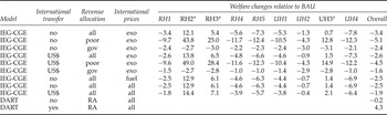
Table 2 provides information on the welfare changes for different scenarios and household types. This reconfirms that different households with different types of factor income and different consumption preferences can be affected very differently by the climate policy induced price changes and transfers. Only when revenues are used for investment purposes are welfare losses relatively equal between households, even though this policy is slightly regressive. International transfers make this pattern even more pronounced; however, they play a smaller role compared to the distribution of the domestic carbon tax revenue.
Changes in accumulated and discounted welfare in selected scenarios

Notes: ‘Overall’ refers to a weighted average (weight by household consumption expenditure) for IEG-CGE and of the representative agent (RA) for DART. Household types marked with an asterisk are considered as poor. See also table A2 in the online appendix for the relative importance of the different variations on overall and poor households' welfare.
As expected, India as a net energy importer benefits from lower fossil fuel prices which reduce the adverse welfare effects. Price changes in other sectors have virtually no additional welfare effect. The welfare gains of price changes are larger under a scenario without transfers because, as discussed above, the exchange rate appreciation caused by transfer payments reduces the benefits of the fuel price effect.
Our results indicate that poor households are most affected by the distribution of revenues. Poor households gain (relative to the BAU) in all scenarios where revenues are allocated to all or poor households. International transfers or taking into account international price repercussions is less important for determining distributive consequences. A decline in the income gap between richer and poorer households comes, however, at the cost of a lower GDP growth rate leading to higher overall welfare losses.
Table 2 also contains welfare changes in DART for two scenarios (with and without international transfers). The most comparable scenarios in IEG-CGE contain transfers to all households and price repercussions in all sectors. Welfare losses in DART are smaller compared to IEG-CGE. With transfers, Indian welfare even increases in DART. Different underlying economic structures and different assumptions about elasticities imply cheaper abatement options in DART than in IEG-CGE. As a consequence, the gains from international transfers are larger in DART because of the larger amount of surplus emissions in DART. Different assumptions on the exchange rate adjustment also contribute to the differences, as in IEG-CGE international transfers lead to an appreciation with reduced welfare gains.
5. Conclusion
For ambitious global climate policies, it is necessary to include India in a global climate regime. There is, however, a fear that this comes at the cost of lower economic growth and that poor households would suffer in particular. Traditional impact analysis of climate mitigation in India has been carried out with single-country models which lack international repercussions or with global models which are highly aggregated for India. This paper shows that both classes of models give an incomplete picture. Soft-linking these two model types can give a more detailed and accurate view for India. The soft-link here is established by harmonizing the models with respect to GDP and population and by passing on price information.
In the global model with only one RA, distributional effects are missing. For India, such effects are crucial for policy makers when assessing the impacts of climate mitigation policy. As the national model shows, welfare effects can differ significantly for different household types so that average welfare numbers are of little use. In addition, redistribution of revenue from a carbon tax and international transfers to poorer households – which cannot be captured in the global model – does benefit the poorer households but comes at the cost of overall higher GDP and welfare losses. The analysis also shows that accounting for international transfers often ignored in national models indeed reduces negative welfare effects for India. Income distribution is furthermore affected by international price repercussions which are also normally not accounted for in national models. By passing on price changes from the global to the national model we show that poor household groups benefit least from lower international fossil fuel prices and also have higher welfare losses when revenues are used for investment which is most efficient in terms of GDP or overall welfare losses. This does not mean that revenues need to be allocated to poor households exclusively; transfers to all households on a per capita basis already make poor households better off than the baseline and reduce the income gap between rich and poor households.
We also see that the rather small negative or even positive welfare effects of international climate policy have to be treated with care. Even though the differences in our model analyses partly stem from different implicit abatement costs, neglecting the exchange rate adjustments and overall welfare effects of different revenue recycling could lead to overly optimistic results in the global model.
While the model soft-linking allows a more detailed view of the distributional effects of international climate policy in India and allows identification of the relative importance of the different channels, the overall consistency of the two models is clearly limited and our scenarios are necessarily highly stylized. For example, other use of the revenues such as financing clean energy or other ‘green technologies’ would be possible but cannot be analyzed in our modeling framework. Also, because of urbanization and industrialization, the household types will probably not correspond to the initial occupation categories in the long run. If interpreted in a more general way as household types of different income levels (derived from different endowment ratios) and different consumption preferences, the results still indicate how rich and poor households are affected under different policy options.
Furthermore, a more complete coupling which could include a further harmonization of the baseline scenarios and potentially also feedback from the Indian model to the global model is challenging for two independently developed models with their own focusses and underlying assumptions. Only a fully integrated model, which could be achieved by splitting the input data of the global model for India, would lead to complete consistency. Such a model would, however, require significant data work. Even though this was beyond the scope of this paper, our results show that it might be worth the effort.
Supplementary materials and methods
The supplementary material referred to in this paper can be found online at journals.cambridge.org/EDE/.