


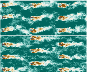



1. Introduction
Tidal stream energy is being developed rapidly as a promising complement to intermittent wind and solar energy, owing to the high predictability of tides (Adcock et al. Reference Adcock, Draper, Willden and Vogel2021). To ensure tidal energy is successfully embedded into the future net-zero carbon energy mix, we need to understand the flow physics driving the efficiency of tidal turbine arrays when deployed at a large scale. Due to the confined flow environment in which these turbines operate, we cannot simply infer tidal array hydrodynamics from existing knowledge of wind farm aerodynamics (Nishino & Dunstan Reference Nishino and Dunstan2020; Porté-Agel, Bastankhah & Shamsoddin Reference Porté-Agel, Bastankhah and Shamsoddin2020). For instance, relatively shallow waters may restrict the ability of turbine wakes to expand vertically, potentially affecting the recovery of wakes in a large array. Effects of vertical mixing between turbine wakes and the atmospheric flow aloft, known to play a key role in large wind farms (Cal et al. Reference Cal, Lebrón, Castillo, Kang and Meneveau2010; Camp & Cal Reference Camp and Cal2016; Bossuyt, Meneveau & Meyers Reference Bossuyt, Meneveau and Meyers2017), are also absent in tidal arrays.
Future tidal arrays will comprise multiple rows of turbines, whose design requires us to consider an appropriate spacing between turbines as well as their impact on the tidal channel flow dynamics. These micro- (turbine-to-turbine) and macro-scale (array-to-tidal channel) interactions need to be considered when designing tidal arrays in order to find the optimal trade-off between energy extraction and minimal changes to the tidal flow (De Dominicis, Wolf & O'Hara Reference De Dominicis, Wolf and O'Hara2018). Large tidal arrays deployed at a tidal channel would lead to an added resistance to its flow dynamics, which, if too large, can considerably obstruct and modify the overall flow. Therefore, to optimise the design of large tidal arrays, it is required to tune the operating conditions of individual turbines for a given tidal channel (e.g. straight or variable-section), tidal forcing and turbine density (Vennell Reference Vennell2010, Reference Vennell2011; Vennell et al. Reference Vennell, Funke, Draper, Stevens and Divett2015).
At the micro-scale, the power production capability of tidal turbines is driven by turbulent wake mixing and acceleration of bypass flow in-between turbines. In relatively closely packed arrays limiting the negative wake-turbine interactions is often key to minimising power losses (Stallard et al. Reference Stallard, Collings, Feng and Whelan2013). However, local blockage due to a small lateral spacing between devices (as well as a shallow water depth confining the flow) may lead to local flow acceleration that enhances individual turbine power, as observed in experimental tests, e.g. Stallard et al. (Reference Stallard, Collings, Feng and Whelan2013) and Noble et al. (Reference Noble, Draycott, Nambiar, Sellar, Steynor and Kiprakis2020). The effect of local blockage has also been investigated using the linear momentum actuator disc theory (LMADT) for a single lateral row of turbines (Garrett & Cummins Reference Garrett and Cummins2007; Nishino & Willden Reference Nishino and Willden2012, Reference Nishino and Willden2013; Vogel, Houlsby & Willden Reference Vogel, Houlsby and Willden2016; Creed et al. Reference Creed, Draper, Nishino and Borthwick2017) and two rows of turbines (Draper & Nishino Reference Draper and Nishino2014). These studies suggest that two staggered rows of turbines tend to be more efficient than two perfectly aligned (or centred) rows of turbines, but less efficient than a single row of the same total number of turbines with the same array width.
Whilst the above findings are important for the performance of arrays with a small number of rows, future tidal arrays will require turbines to be deployed in several rows to generate a sufficiently large amount of energy, which may cause macro-scale flow interactions between the array and the tidal channel. Vennell (Reference Vennell2010, Reference Vennell2011) combined the LMADT with a simple theoretical tidal channel flow model to analyse how the resistance and lateral spacing of turbines within each row should be tuned for a given number of rows deployed across a given tidal channel, to maximise the total power generation. However, existing theoretical tidal array models based on the LMADT, including the two-row model of Draper & Nishino (Reference Draper and Nishino2014), do not fully account for the complex effect of turbulent wake mixing. The Vennell-type array models assume that the streamwise spacing between rows is large enough for individual turbine wakes to be fully mixed after each row, whereas the two-row model of Draper & Nishino (Reference Draper and Nishino2014) assumes that the two rows are close enough to each other for the effect of wake mixing to be negligible.
In narrow tidal channels or straits turbines in a multi-row array may operate in a fully waked scenario (similar to a perfectly aligned layout) during half of the tidal cycle (e.g. ebb tide), but they may operate in partly waked conditions (akin to staggered layouts) during the other half of the cycle (e.g. flood tide) (Garcia Novo & Kyozuka Reference Garcia Novo and Kyozuka2019). This asymmetry between ebb and flood tide directions further complicates the design of optimal array configurations, requiring us to understand the performance and hydrodynamics of a given array design for various incident flow characteristics. Many existing studies looking into tidal array optimisation have adopted low-fidelity flow models, such as two-dimensional shallow water models (Culley et al. Reference Culley, Funke, Kramer and Piggott2018), analytical wake models, e.g. Gaussian models (Stansby & Stallard Reference Stansby and Stallard2015) and aforementioned theoretical models based on the LMADT (Nishino & Willden Reference Nishino and Willden2013; Draper & Nishino Reference Draper and Nishino2014), while high-fidelity simulations have been restricted to relatively small arrays with a limited number of configurations, due to their large computational expense (Afgan et al. Reference Afgan, McNaughton, Rolfo, Apsley, Stallard and Stansby2013; Chawdhary et al. Reference Chawdhary, Hill, Yang, Guala, Corren, Colby and Sotiropoulos2017; Ouro, Ramírez & Harrold Reference Ouro, Ramírez and Harrold2019c). However, as the performance of tidal devices in arrays is driven by wake-turbine interactions as well as bathymetry-induced turbulence (Stallard et al. Reference Stallard, Collings, Feng and Whelan2013; Ouro & Stoesser Reference Ouro and Stoesser2019), turbulence-resolving approaches such as large-eddy simulation (LES) are valuable to yield reliable hydrodynamics results as well as to build more accurate low-order models that can improve array optimisation tools.
In this paper we investigate the flow characteristics and efficiency of infinitely large tidal arrays with perfectly aligned and staggered configurations, combining predictions from two contrasting approaches: actuator disc theory and LES. An infinitely large array represents an asymptotic case in which the flow passing the turbine rows is fully developed (i.e. flow statistics become identical for all rows). This is similar to large wind farms in which such flow conditions may be attained approximately after 10 to 15 rows, depending on the atmospheric stability conditions (Bossuyt et al. Reference Bossuyt, Meneveau and Meyers2017; Sharma et al. Reference Sharma, Cortina, Margairaz, Parlange and Calaf2018; Porté-Agel et al. Reference Porté-Agel, Bastankhah and Shamsoddin2020). We consider a wide range of streamwise and lateral turbine spacing to understand how the array efficiency can be maximised (from the micro-scale perspective) by balancing the negative impact of turbine wakes impinging downstream turbines and the positive local blockage effects. The paper is structured as follows. In § 2 we introduce an extended theoretical model developed for periodic turbine arrays with perfectly aligned and staggered configurations. Details of the 28 LES runs comprising aligned and staggered layouts are presented in § 3, with results of flow characteristics, hydrodynamic coefficients and turbine loading unsteadiness in § 4. In § 5 we provide further discussion on the comparison between the predictions obtained from the theoretical analysis and LES, followed by main conclusions in § 6.
2. Theoretical analysis
We start with a simple theoretical analysis on the efficiency of an infinitely large array of ideal turbines in a steady, uniform and vertically confined flow. The analysis is based on the work of Draper & Nishino (Reference Draper and Nishino2014), who extended the LMADT for laterally confined flows (Garrett & Cummins Reference Garrett and Cummins2007; Houlsby, Draper & Oldfield Reference Houlsby, Draper and Oldfield2008) to predict an upper limit to the efficiency of two aligned or staggered rows of turbines. This two-row analysis is further extended in this study to investigate an infinite number of aligned or staggered rows of tidal turbines, following the idea of the hybrid inviscid-viscous approach recently proposed by Nishino & Draper (Reference Nishino and Draper2019).
Figure 1 illustrates an example of a periodic staggered array of tidal turbines. The key assumption employed in the hybrid inviscid-viscous approach is that the streamwise extent of the region in which the expansion of the flow through each turbine takes place is much shorter than the distance between each row of turbines. With this assumption, we hypothetically divide the flow field into two types of zones; namely the inviscid flow zones, which are analysed using the LMADT neglecting the effect of viscous (or turbulent) mixing, and the viscous flow zones, which are modelled separately to account for the effect of mixing. This approach is also in line with the results of a recent LES study of flow past a periodic array of actuator discs (West & Lele Reference West and Lele2020) showing that the effects of inviscid and viscous (turbulent) flow processes are dominant, respectively, in the vicinity of the turbines and in the rest of the flow field.
Schematic of the flow past a periodic staggered array of tidal turbines, divided into the hypothetical inviscid (inv.) and viscous (visc.) flow zones. The rectangular region enclosed by the magenta dashed line corresponds to that depicted in figure 2.

Although we refer to this periodic flow problem as an ’infinitely large’ array problem, the analysis presented below is still relevant to finite-size tidal arrays to be built in the future. The key conditions that would need to be satisfied (for the analysis to be directly relevant) are: (i) the number of turbine rows is large enough for the flow through the array to reach (approximately) a ‘fully developed’ state; and (ii) the array occupies the entire width of a given tidal channel so that the incoming flow will not expand laterally to bypass the whole array. For the first condition, the number of rows required could be relatively small for tidal arrays (compared with that for wind farms) as the flow is vertically confined, whereas the second condition means that the number of turbines in each row could also be relatively small if the channel is narrow. Hence, this ‘infinitely large’ array study could be relevant to even medium-sized tidal arrays.
In this study we consider that the mass flow rate through the array is constant and not affected by the resistance caused by the array. In reality, the mass flow rate would be affected by the array if the number of rows is large enough for the array-induced resistance to become non-negligible compared with the natural resistance of the channel. Such a scenario could be studied if the analysis presented below is combined with, for example, a channel-scale momentum balance model (Vennell Reference Vennell2010). The analysis may also be combined with a shallow channel flow model (Creed et al. Reference Creed, Draper, Nishino and Borthwick2017) to study the array performance in a laterally unconfined (or less confined) situation, where the effect of bed friction becomes important as it affects how the incoming flow expands laterally to bypass the whole array. However, these channel-scale effects are outside the scope of the present study, as our main focus here is on the effect of turbine layout on ‘local’ power characteristics of turbines within a fully developed region of an array (i.e. power of turbines for a given mass flow rate).
2.1. Staggered rows of actuator discs
A schematic of the theoretical model for the staggered case is shown in figure 2. Here we consider a straight local flow passage containing only one-half of an actuator disc due to the periodic and symmetric nature of the array as shown in figure 1. The cross-sectional area of the flow passage is  $A/B$, where
 $A$ is the half-disc area and
 $B$ is the area blockage ratio. Although the figure is depicted in a two-dimensional manner, this is still a quasi-one-dimensional flow model as we do not consider any variation of flow quantities (velocity and pressure) over the cross-section of each streamtube in the inviscid zone. Assuming that the flow is incompressible, the average velocity over the cross-section of the entire flow passage,
 $u_{av}$, does not change in the streamwise direction.
Schematic of the quasi-one-dimensional theoretical model for a periodic staggered array of tidal turbines, with examples of how cross-sectional flow patterns may appear in a corresponding three-dimensional flow problem. The three vertical thin black lines in the top and middle drawings indicate the locations of stations 1, 4 and 5. In the middle drawing these thin black lines also indicate the (non-dimensional) cross-sectional average velocity,  $\psi = u_{av}/u_{ref}$, for the superposed plot of
 $u/u_{ref}$ at each station, whereas the thick black lines show example profiles of
 $u/u_{ref}$ at the three stations (calculated for the case with
 $B=0.2$,
 $K=3$ and
 $m=0.7$). Reproduced from Nishino & Draper (Reference Nishino and Draper2019) with modifications.

Following the common notations used in the LMADT (Houlsby et al. Reference Houlsby, Draper and Oldfield2008) we define four stations within the inviscid zone: station 1 is at the inlet of the inviscid zone where the core-flow streamtube (that encompasses the actuator disc) starts to expand, stations 2 and 3 are immediately upstream and downstream of the disc, respectively, and station 4 is at the outlet of the inviscid zone where the pressure is equalised between the core- and bypass-flow streamtubes. In addition, we describe the outlet of the viscous zone as station 5 (which is station 1 for the next row of discs). The pressure at stations 1 to 5 is denoted by  $p_1$ to
 $p_5$, respectively, whereas the velocity is described using the velocity coefficients
 $\alpha$ and
 $\beta$ with subscripts as in figure 2. Each velocity coefficient represents the ratio of the velocity there to a reference velocity,
 $u_{ref}$. In the following we take the core-flow velocity at station 1 as
 $u_{ref}$ (i.e.
 $\alpha _1 = 1$) for convenience.
We now consider the conservation of mass, momentum and energy in the inviscid flow zone in a similar manner to the work of Draper & Nishino (Reference Draper and Nishino2014). First, since the Bernoulli equation must be satisfied to conserve energy in each of the three bypass-flow streamtubes between stations 1 and 4, we obtain
 \begin{gather} p_1-p_4 = \tfrac{1}{2}\rho u_{ref}^{2} \left( \beta_{4a}^{2}-1 \right), \end{gather}
 \begin{gather}p_1-p_4 = \tfrac{1}{2}\rho u_{ref}^{2} \left( \beta_{4b}^{2}-\beta_5^{2} \right), \end{gather}
 \begin{gather}p_1-p_4 = \tfrac{1}{2}\rho u_{ref}^{2} \left( \alpha_8^{2}-\alpha_5^{2} \right), \end{gather}
where  $\rho$ is the fluid density. Substituting (2.2) and (2.3), respectively, into (2.1) gives
 \begin{gather} \beta_{4b} = \left( \beta_{4a}^{2} + \beta_{5}^{2} - 1 \right)^{1/2}, \end{gather}
 \begin{gather}\alpha_{8} = \left( \beta_{4a}^{2} + \alpha_{5}^{2} - 1 \right)^{1/2}. \end{gather}
As the Bernoulli equation must also be satisfied in the upstream part (between stations 1 and 2) and downstream part (between stations 3 and 4) of the core-flow streamtube, we also obtain
 \begin{equation} p_2-p_3 = p_1-p_4 + \tfrac{1}{2}\rho u_{ref}^{2} \left( 1-\alpha_4^{2} \right), \end{equation}
which, together with (2.1), leads to an expression for the half-disc thrust,  $T$, as
 \begin{equation} T = (p_2-p_3)A = \tfrac{1}{2}\rho u_{ref}^{2} A \left( \beta_{4a}^{2} - \alpha_4^{2} \right), \end{equation}
and, thus, an expression for the half-disc power,  $P$, as
 \begin{equation} P = T\alpha_2 u_{ref} = \tfrac{1}{2}\rho u_{ref}^{3} A \alpha_2\left( \beta_{4a}^{2} - \alpha_4^{2} \right). \end{equation}
Hence, to obtain  $P$ for a given
 $\alpha _2$, for example, we need to know how
 $\alpha _4$ and
 $\beta _{4a}$ depend on
 $\alpha _2$. By considering the conservation of mass in the ‘main’ bypass-flow streamtube between station 1 (where the velocity is
 $\beta _5 u_{ref}$) and station 4 (where the velocity is
 $\beta _{4b} u_{ref}$) we obtain
 \begin{equation} \beta_5 u_{ref} A \left(\frac{1}{B} - \frac{\alpha_2}{\alpha_4} - \gamma \right) = \beta_{4b} u_{ref} A \left(\frac{1}{B} - \frac{\alpha_2}{\alpha_4} - \frac{\gamma - \alpha_2}{\beta_{4a}} - \gamma \right), \end{equation}
which leads to
 \begin{equation} \alpha_4 = \frac{\alpha_2}{\dfrac{1}{B} - \dfrac{\beta_{4b}}{\beta_{4a}} \left(\dfrac{\gamma - \alpha_2}{\beta_{4b} - \beta_5} \right) - \gamma}, \end{equation}
where
 \begin{equation} \gamma = \frac{\alpha_2 \alpha_5}{\alpha_4 \alpha_8} \end{equation}
is the area ratio for the wake flow upstream of the disc as depicted in figure 2. Note that this wake originates from the disc located two rows upstream (and its velocity increases from  $\alpha _5 u_{ref}$ to
 $\alpha _8 u_{ref}$ when it passes through the row immediately upstream) due to the staggered configuration. As for
 $\beta _{4a}$, we consider the conservation of momentum for the entire flow passage to obtain
 \begin{align} (p_1 - p_4)\frac{A}{B} - T &= \rho u_{ref}^{2} A \left[ \alpha_2 (\alpha_4 - 1) + (\gamma - \alpha_2)(\beta_{4a} - 1) + \gamma \alpha_8(\alpha_8 - \alpha_5) \vphantom{\left( \frac{1}{B} -\frac{\alpha_2}{\alpha_4} -\gamma \right)}\right.\nonumber\\ &\quad \left.+ \beta_5 \left( \frac{1}{B} - \frac{\alpha_2}{\alpha_4} -\gamma \right) \left( \beta_{4b} - \beta_5 \right)\right], \end{align}
which, together with (2.1) and (2.7), leads to
 \begin{align} & \left( 1-B \right)\beta_{4a}^{2} - 2B \left( \gamma-\alpha_2 \right) \beta_{4a} - 2B \left[ \alpha_2 \alpha_4 - \frac{1}{2}\alpha_4^{2} + \gamma \left( \alpha_8^{2} - \alpha_5 \alpha_8 - 1 \right) \right] \nonumber\\ &\quad -2\beta_5 \left( \beta_{4b} - \beta_5 \right) \left[ 1-B \left( \frac{\alpha_2}{\alpha_4} + \gamma \right) \right] - 1 = 0. \end{align}
The above set of equations for the inviscid zone is not closed as it includes  $\alpha _5$ and
 $\beta _5$, which need to be modelled considering the effect of mixing in the viscous zone. There are several possible ways to model the effect of mixing but here we employ a very simple approach using a single non-dimensional input parameter called the mixing factor,
 $m$, which represents the completeness of mixing in the viscous zone. Specifically, the value of
 $m$ (between 0 and 1) describes how much the velocity of flow at each cross-sectional position returns to the cross-sectional average velocity of the entire flow passage,
 $u_{av}$, as the flow passes through the viscous zone. By applying this to the wake flow of the disc we obtain
 \begin{equation} \alpha_5 = m\psi + \left( 1-m \right) \alpha_4 , \end{equation}
where  $\psi = u_{av}/u_{ref}$ is the non-dimensional cross-sectional average velocity and this can be calculated from the velocity profile at station 1, for example, as
 \begin{equation} \psi = B \left[ \gamma \left( \alpha_8 + 1 \right) + \beta_5 \left( \frac{1}{B} - \frac{\alpha_2}{\alpha_4} - \gamma \right) \right] . \end{equation}
For the bypass flow, however, the difficulty is that the number of flow passages at station 4 does not agree with that at station 1, since the actuator disc creates the additional narrow bypass streamtube that has  $\beta _{4a}$ at station 4. To obtain a closed set of equations for this periodic flow problem within the framework of quasi-one-dimensional modelling, here we assume that the narrow bypass flow immediately outside of the wake is ‘merged’ or fully mixed with the main bypass flow regardless of the value of
 $m$. This assumption seems reasonable since the difference between
 $\beta _{4a}$ and
 $\beta _{4b}$ tends to be small as depicted in figure 2, and eventually leads to
 \begin{equation} \beta_5 = m\psi + \left( 1-m \right) \beta_{4m}, \end{equation}
where  $\beta _{4m}$ is the ‘area-weighted’ average of
 $\beta _{4a}$ and
 $\beta _{4b}$, i.e.
 \begin{equation} \beta_{4m} = \frac{\left( \gamma - \alpha_2 \right) + \beta_5\left(\dfrac{1}{B} - \dfrac{\alpha_2}{\alpha_4} - \gamma \right)}{\dfrac{\left( \gamma - \alpha_2 \right)}{\beta_{4a}} + \dfrac{\beta_5}{\beta_{4b}} \left( \dfrac{1}{B} - \dfrac{\alpha_2}{\alpha_4} - \gamma \right)} . \end{equation}
It should be noted that  $\alpha _9 = m\psi + ( 1-m ) \alpha _8$ is required together with (2.14) to (2.17) to conserve the total mass in the viscous zone, but this is automatically satisfied as we enforce
 $\alpha _9=\alpha _1=1$ in this analysis due to the periodicity of the flow.
Finally, the thrust and power coefficients of the disc are expressed (for a given cross-sectional average velocity of the entire flow,  $u_{av}=\psi u_{ref}$) as
 \begin{gather} C_T = \frac{T}{\dfrac{1}{2}\rho \left( \psi u_{ref} \right)^{2} A} = \frac{\beta_{4a}^{2} - \alpha_4^{2}}{\psi^{2}}, \end{gather}
 \begin{gather}C_P = \frac{P}{\dfrac{1}{2}\rho \left( \psi u_{ref} \right)^{3} A} = \frac{\alpha_2\left( \beta_{4a}^{2} - \alpha_4^{2} \right)}{\psi^{3}}. \end{gather}
For convenience, we also define the resistance coefficient (or local thrust coefficient) of the disc as
 \begin{equation} K = \frac{T}{\dfrac{1}{2}\rho \left( \alpha_2 u_{ref} \right)^{2} A} , \end{equation}
from which and (2.7), we obtain
 \begin{equation} \alpha_2 = \left( \frac{\beta_{4a}^{2} - \alpha_4^{2}}{K} \right)^{1/2} . \end{equation}
In summary, the above theoretical model for an infinite number of staggered rows of identical ideal turbines consists of three non-dimensional input parameters ( $B$,
 $K$,
 $m$), ten non-dimensional unknowns to be determined (
 $\alpha _2$,
 $\alpha _4$,
 $\alpha _5$,
 $\alpha _8$,
 $\beta _{4a}$,
 $\beta _{4b}$,
 $\beta _{4m}$,
 $\beta _5$,
 $\gamma$,
 $\psi$) and a set of ten equations to be solved numerically: (2.4), (2.5), (2.10), (2.11), (2.13), (2.14), (2.15), (2.16), (2.17) and (2.21).
2.2. Aligned rows of actuator discs
Compared with the staggered case, the theoretical model for the aligned case becomes simpler as only two bypass-flow streamtubes (instead of three) need to be considered in the inviscid zone. This is because the wake encounters the disc immediately downstream (instead of two rows downstream). In the following, we again consider the conservation of mass, momentum and energy in the inviscid zone, and the simplified mixing process in the viscous zone, to derive a similar but smaller set of equations for the aligned case.
By applying the Bernoulli equation to the two bypass-flow streamtubes and the core-flow streamtube in the same manner as in the staggered case, we obtain (2.1), (2.2) and (2.6), which lead to (2.4), (2.7) and (2.8) for  $\beta _{4b}$,
 $T$ and
 $P$, respectively. Note that these equations are identical for both aligned and staggered cases, whereas (2.3) and (2.5) are only for the staggered case (since the third bypass-flow streamtube does not exist in the aligned case). Next, from the conservation of mass in the ‘main’ bypass-flow streamtube, we obtain
 \begin{equation} \beta_5 u_{ref} A \left(\frac{1}{B} - \frac{\alpha_2}{\alpha_4} \right) = \beta_{4b} u_{ref} A \left[\frac{1}{B} - \frac{\alpha_2}{\alpha_4} - \frac{1}{\beta_{4a}}\left( \frac{\alpha_2}{\alpha_4}-\alpha_2 \right) \right], \end{equation}
which leads to an expression for  $\alpha _4$ as
 \begin{equation} \alpha_4 = \frac{\alpha_2 \left( 1 + \dfrac{1}{\beta_{4a}} - \dfrac{\beta_5}{\beta_{4b}} \right)}{\dfrac{1}{B}\left( 1 - \dfrac{\beta_5}{\beta_{4b}} \right) + \dfrac{\alpha_2}{\beta_{4a}} }. \end{equation}
For  $\beta _{4a}$, we consider the conservation of momentum for the entire flow to obtain
 \begin{align} & (p_1 - p_4)\frac{A}{B} - T \nonumber\\ &\quad = \rho u_{ref}^{2} A \left[ \alpha_2 (\alpha_4 - 1) + \left( \frac{\alpha_2}{\alpha_4} - \alpha_2 \right)(\beta_{4a} - 1) + \beta_5 \left( \frac{1}{B} - \frac{\alpha_2}{\alpha_4} \right) \left( \beta_{4b} - \beta_5 \right) \right] , \end{align}
which, together with (2.1) and (2.7), leads to
 \begin{align} & \left( 1-B \right)\beta_{4a}^{2} - 2B \left( \frac{\alpha_2}{\alpha_4}-\alpha_2 \right) \beta_{4a} - 2B \left( \alpha_2 \alpha_4 - \frac{1}{2}\alpha_4^{2} - \frac{\alpha_2}{\alpha_4} \right) \nonumber\\ &\quad -2\beta_5 \left( \beta_{4b} - \beta_5 \right) \left( 1-B \frac{\alpha_2}{\alpha_4} \right) - 1 = 0. \end{align}
For  $\beta _5$, we need to consider the effect of mixing in the viscous zone. By employing the same approach as in the staggered case, we obtain (2.16) for the aligned case as well. Note, however, that
 $\psi$ and
 $\beta _{4m}$ are different for the aligned case, which are
 \begin{equation} \psi = B \left[ \frac{\alpha_2}{\alpha_4} + \beta_5 \left( \frac{1}{B} - \frac{\alpha_2}{\alpha_4} \right) \right] , \end{equation}
and
 \begin{equation} \beta_{4m} = \frac{\left( \dfrac{\alpha_2}{\alpha_4} - \alpha_2 \right) + \beta_5 \left( \dfrac{1}{B} - \dfrac{\alpha_2}{\alpha_4} \right)}{\dfrac{1}{\beta_{4a}} \left( \dfrac{\alpha_2}{\alpha_4} - \alpha_2 \right) + \dfrac{\beta_5}{\beta_{4b}} \left( \dfrac{1}{B} - \dfrac{\alpha_2}{\alpha_4} \right)} . \end{equation}
We also need (2.14) together with the above equations to conserve the total mass in the viscous zone, but this is automatically satisfied since here we enforce  $\alpha _5=\alpha _1=1$ due to the periodicity of the flow. Finally,
 $C_T$,
 $C_P$ and
 $K$ are all defined as in the staggered case, yielding the same equations (2.18) to (2.20) and, thus, (2.21) for
 $\alpha _2$.
In summary, the theoretical model for the aligned case consists of three non-dimensional input parameters ( $B$,
 $K$,
 $m$), seven non-dimensional unknowns (
 $\alpha _2$,
 $\alpha _4$,
 $\beta _{4a}$,
 $\beta _{4b}$,
 $\beta _{4m}$,
 $\beta _5$,
 $\psi$) and a set of seven equations to be solved numerically: (2.4), (2.16), (2.21), (2.23), (2.25), (2.26) and (2.27).
2.3. Example solutions
Here we present some example solutions of the above theoretical model, first for the aligned case and then for the staggered case. As this is a three-parameter ( $B$–
 $K$–
 $m$) problem, we start with fixing the disc resistance coefficient,
 $K$, at its optimal value for the complete mixing case, i.e.
 $m=1$. When
 $m=1$, our problem (for both aligned and staggered cases) reduces to the two-parameter (
 $B$–
 $K$) problem of Garrett & Cummins (Reference Garrett and Cummins2007) (hereafter referred to as GC07); hence, this optimal value for
 $m=1$ is known to be
 $K=2(1+B)^{3}/(1-B)^{2}$, which we refer to as
 $K_\mathrm {GC07}$.
Figure 3 shows how the performance of aligned rows of such ‘suboptimal’ actuator discs (with  $K=K_\mathrm {GC07}$) changes with
 $m$, at two different blockage ratios,
 $B=0.05$ and
 $0.2$. As can be expected intuitively, the power coefficient
 $C_P$ of aligned discs decreases monotonically as the mixing factor
 $m$ decreases (regardless of the blockage ratio). This agrees with the common observation that the power of aligned rows of turbines tends to decrease as we reduce the streamwise spacing between the rows, noting that the mixing tends to be less complete (i.e.
 $m$ tends to be small) when the spacing is small.
Theoretical prediction of the effect of mixing on the performance of aligned rows of actuator discs at two different blockage ratios: (a)  $B=0.05$ and (b)
 $B=0.2$. The disc resistance coefficient is fixed at the optimal value for the case with complete mixing (
 $m=1$), i.e.
 $K=2(1+B)^{3}/(1-B)^{2}$.

We also present in figure 3 the values of  $\alpha _2(\beta _{4a}^{2}-\alpha _4^{2})$ and
 $1/\psi ^{3}$, to explain why
 $C_P$ decreases as
 $m$ decreases. As can be seen from (2.19),
 $C_P$ is equivalent to the product of these two values; the former is a different power coefficient defined using the velocity upstream of the disc (
 $u_{ref}$) instead of the cross-sectional average velocity (
 $u_{av}$), and the latter represents the effect of the difference between
 $u_{ref}$ and
 $u_{av}$. Here we can see that the value of
 $\alpha _2(\beta _{4a}^{2}-\alpha _4^{2})$ actually increases as
 $m$ decreases. This is essentially because the local blockage effect is enhanced (or the ‘effective’ blockage ratio increases) when the upstream core flow is slower than the upstream bypass flow (Draper et al. Reference Draper, Nishino, Adcock and Taylor2016). This enhancement of the local blockage effect caused by the incomplete wake mixing of the upstream disc, however, is not strong enough to compensate for the ‘loss’ of power possessed by the upstream core flow compared with the ‘original’ power possessed by the cross-sectionally averaged flow (i.e. the increase rate of
 $\alpha _2(\beta _{4a}^{2}-\alpha _4^{2})$ is smaller than the decrease rate of
 $1/\psi ^{3}$); therefore,
 $C_P$ eventually decreases as
 $m$ decreases.
Although the above analysis was for ‘suboptimal’ discs with  $K=K_\mathrm {GC07}$, the same relationship between
 $C_P$ and
 $m$ is generally found for aligned discs with any given
 $K$ values. Figures 4(a) and 4(b) show
 $C_P$ vs
 $K$ curves for five different
 $m$ values, again at
 $B=0.05$ and
 $0.2$, respectively, demonstrating the trend. It can also be seen that the optimal
 $K$ value (to maximise
 $C_P$) tends to decrease as
 $m$ decreases, although the
 $C_P$ obtained at
 $K=K_\mathrm {GC07}$ is still close to the maximum
 $C_P$ for a given
 $m$ (especially when the blockage ratio is high). Figure 4(c) shows how the maximum
 $C_P$, or
 $C_{P{max}}$, changes with
 $m$. As can be expected, for aligned rows of actuator discs,
 $C_{P{max}}$ also decreases monotonically as
 $m$ decreases. Figure 5 shows
 $C_P$ vs
 $C_T$ curves for the same five different
 $m$ values as in figures 4(a) and 4(b), again at
 $B=0.05$ and
 $0.2$. The same trend can be confirmed here as well.
Theoretical  $C_P$ vs
 $K$ for the aligned case at (a)
 $B=0.05$ and (b)
 $B=0.2$; and (c) the maximum
 $C_P$ obtained by varying
 $K$ for a given set of
 $B$ and
 $m$.

Theoretical  $C_P$ vs
 $C_T$ for the aligned case at (a)
 $B=0.05$ and (b)
 $B=0.2$.

Next, we focus on staggered rows of actuator discs. Similarly to the aligned case, we start with the performance of ‘suboptimal’ discs with  $K=K_\mathrm {GC07}$, which is shown in figures 6(a) and 6(b) for
 $B=0.05$ and
 $0.2$, respectively. At
 $B=0.05$, the value of
 $1/\psi ^{3}$ slightly increases (meaning that the upstream core-flow velocity becomes slightly higher than the cross-sectional average velocity) as
 $m$ decreases from 1 to about 0.95, and then decreases as
 $m$ further decreases. In contrast, the value of
 $\alpha _2(\beta _{4a}^{2}-\alpha _4^{2})$ first decreases slightly and then increases as
 $m$ decreases from 1; this is again due to changes in the ‘effective’ blockage ratio, i.e. the local blockage effect is enhanced (or diminished) when the upstream core flow is surrounded by a faster (or slower) bypass flow. However, the increase (or decrease) rate of
 $\alpha _2(\beta _{4a}^{2}-\alpha _4^{2})$ tends to be smaller than the decrease (or increase) rate of
 $1/\psi ^{3}$, and, hence,
 $C_P$ follows the trend of
 $1/\psi ^{3}$, i.e.
 $C_P$ slightly increases first and then decreases as
 $m$ decreases from 1. This initial increase in
 $1/\psi ^{3}$ (and, thus, in
 $C_P$) is more clearly seen at
 $B=0.2$, demonstrating that the beneficial effect of the staggered layout (allowing the velocity upstream of the disc to become higher than the cross-sectional average velocity) is enhanced at a higher blockage ratio.
Theoretical prediction of the performance of staggered rows of actuator discs: the effect of mixing at (a)  $B=0.05$ and (b)
 $B=0.2$; and (c) comparison of
 $C_P$ vs
 $B$ between the complete mixing case (
 $m=1$) and optimal mixing case (
 $m=m_{C_P}$). Plotted together are
 $m_{C_P}$ and
 $m_{\psi }$, which are the values of
 $m$ to maximise
 $C_P$ and to minimise
 $\psi$, respectively. The disc resistance coefficient is fixed at the optimal value for
 $m=1$, i.e.
 $K=2(1+B)^{3}/(1-B)^{2}$.

Figure 6(c) compares  $C_P$ vs
 $B$ curves for the complete mixing case (
 $m=1$) and for the ‘optimal mixing’ case (
 $m=m_{C_P}$, where
 $m_{C_P}$ is the value of
 $m$ that maximises
 $C_P$), again for staggered rows of ‘suboptimal’ discs (
 $K=K_\mathrm {GC07}$). Also plotted together are
 $m_{C_P}$ and
 $m_{\psi }$, the latter of which represents the value of
 $m$ that minimises
 $\psi$ (and, thus, maximises
 $1/\psi ^{3}$). It can be seen how the increase in
 $C_P$ due to the beneficial effect of the staggered layout is enhanced, and how the optimal level of mixing decreases, as we increase the blockage ratio. It is also worth noting that the difference between
 $m_{C_P}$ and
 $m_{\psi }$ is small, especially at low blockage ratios. This reflects the dominant influence of
 $1/\psi ^{3}$ on
 $C_P$ as described earlier in figures 6(a) and 6(b).
The  $C_P$ values presented above are for ‘suboptimal’ discs (with
 $K=K_\mathrm {GC07}$) and can therefore be increased further by adjusting
 $K$ for a given
 $m$ (or for a given streamwise distance between the rows). However, this additional increase in
 $C_P$ achieved by varying
 $K$ is rather small for the staggered case. Figures 7(a) and 7(b) show
 $C_P$ vs
 $K$ curves for five different
 $m$ values, again at
 $B=0.05$ and
 $0.2$, respectively. When
 $B$ is small,
 $K_\mathrm {GC07}$ tends to be already close to the optimal
 $K$ value for a given
 $m$; hence, the benefit of further adjusting
 $K$ is small. When
 $B$ is large,
 $K_\mathrm {GC07}$ is not so close to the optimal
 $K$ for a given
 $m$, but the
 $C_P$ vs
 $K$ curve tends to have a flatter peak; hence again, the additional gain in
 $C_P$ by adjusting
 $K$ is small. Figure 7(c) shows the maximum
 $C_P$ (achieved by adjusting
 $K$) vs
 $m$ curves for five different blockage ratios. The curves for
 $B=0.05$ and
 $0.2$ are in fact very similar to the
 $C_P$ vs
 $m$ curves for
 $K=K_\mathrm {GC07}$ plotted earlier in figures 6(a) and 6(b). At
 $B=0.2$, for example, the highest
 $C_P$ value achieved with
 $K=K_\mathrm {GC07}$ is only 1.1 % lower than that achieved by optimising
 $K$. The impact of
 $m$ on
 $C_P$ can also be confirmed from the
 $C_P$ vs
 $C_T$ curves in figure 8, plotted for the same sets of
 $m$ and
 $B$ as in figures 7(a) and 7(b).
Theoretical  $C_P$ vs
 $K$ for the staggered case at (a)
 $B=0.05$ and (b)
 $B=0.2$; and (c) the maximum
 $C_P$ obtained by varying
 $K$ for a given set of
 $B$ and
 $m$.

Theoretical  $C_P$ vs
 $C_T$ for the staggered case at (a)
 $B=0.05$ and (b)
 $B=0.2$.

In summary, these example solutions of the simple three-parameter ( $B$–
 $K$–
 $m$) theoretical model suggest the following. (i) For an infinitely large staggered array of tidal turbines, there is an optimal streamwise turbine spacing (for a given cross-sectional blockage ratio or a given lateral turbine spacing) to maximise the power of each turbine relative to the power of cross-sectional average flow. This is an outcome of the combined effects of local blockage and wake mixing, i.e. this optimum exists because the local flow velocity upstream of each disc can become higher than the cross-sectional average velocity (and this does help to increase the relative power despite reducing the ‘effective’ blockage ratio) when the streamwise turbine spacing is reasonably (not excessively) large for the wake mixing behind each disc to be largely (but not entirely) completed. (ii) The optimal turbine resistance to maximise this relative power also depends on both lateral and streamwise turbine spacing, but the optimal value for a single row, namely
 $K=2(1+B)^{3}/(1-B)^{2}$, is expected to yield close to the maximum relative power. (iii) For an infinitely large aligned array of tidal turbines, however, this relative power is maximised simply when the streamwise turbine spacing is large enough for the wake mixing to be entirely completed; hence, the optimal turbine resistance becomes identical to that for a single row.
Finally, it should be remembered that, in a real tidal array to be built in the future, the cross-sectional average velocity (which was considered as a fixed parameter in the above analysis) would depend on how the flow resistance caused by the entire array alters the natural tidal channel-scale momentum balance (see, e.g. Vennell Reference Vennell2012; Vennell et al. Reference Vennell, Funke, Draper, Stevens and Divett2015; Gupta & Young Reference Gupta and Young2017). As the additional resistance caused by the array would reduce the mass flow rate through the array, the turbine resistance required to maximise the power for a given ‘natural’ mass flow rate (observed in the ‘natural’ channel without the array) would be lower than the optimal resistance discussed above. It should also be noted that, in the real world, tidal currents are oscillatory and, thus, it would be beneficial to vary the turbine resistance during the tidal cycle (Vennell & Adcock Reference Vennell and Adcock2014).
3. Large-eddy simulation set-up
The theoretical model presented above has been developed on the assumption that the flow around each turbine is inviscid and steady. However, real turbine wakes are unsteady with coherent flow structures developed at a rotor level (e.g. tip vortices) and further downstream (e.g. wake meandering). Thus, we now investigate how the theoretical predictions of the performance of infinitely large tidal arrays compare to high-fidelity numerical predictions using LES. We adopt the well-validated in-house LES code digital offshore farms simulator (DOFAS) in which turbine blades are represented using an actuator line method (ALM) (Ouro et al. Reference Ouro, Ramírez and Harrold2019c) and the flow solver is fully parallelised using the message passing interface (MPI), providing a great computational scalability and performance (Ouro et al. Reference Ouro, Fraga, Lopez-Novoa and Stoesser2019a). Details of the flow solver are provided in Appendix A.
We intentionally set the flow conditions to be as similar as possible to the conditions considered in the theoretical analysis, whilst ensuring that the physical dimensions of the turbines are close to those found in real tidal stream turbines. The 1 MW DeepGen IV tidal stream turbine design from the ReDAPT project is adopted, and the details of the blade hydrodynamic data used in the ALM are available in Scarlett et al. (Reference Scarlett, Sellar, van den Bremer and Viola2019). The turbines have a diameter ( $D$) of 12 m, rotating at a constant speed that corresponds to a tip-speed ratio of 4.0 (which is known to be optimal for the case of single-turbine operation), and include 10 m long (
 $0.8D$) nacelles. For convenience, we set the cross-sectional average velocity
 $U_0$ to 2.0 m s
 $^{-1}$ and consider this as our reference velocity, which yields a rotational speed of
 $\varOmega = 1.35$ rad s
 $^{-1}$ and a full-revolution period of
 $T = 4.724$ s.
The computational domain is 432 m long ( $L$), 144 m wide (
 $W$) and 24 m high (
 $H$), equivalent to
 $36D \times 12D \times 2D$, which is close to
 $6{\rm \pi} H \times 2{\rm \pi} H \times H$ commonly used in turbulent channel flow simulations. Turbines are vertically centred at mid-water depth, i.e.
 $z=H/2$, to reduce vertical asymmetry effects that may complicate the comparison between LMADT and LES. The corresponding Froude number (Fr
 $=U_0/\sqrt {gH}$, with
 $g$ denoting the gravitational acceleration) is equal to 0.13, which, together with the given rotor size relative to the water depth, is deemed small enough to ignore any water surface deformation in this study (Houlsby & Vogel Reference Houlsby and Vogel2017; Yan et al. Reference Yan, Deng, Korobenko, Bazilevs and Vogel2017). A fixed time step
 ${\rm \Delta} t$ is set to 0.045 s together with a uniform spatial resolution
 ${\rm \Delta} x$ equal to 0.25 m, yielding a total of 48 mesh elements across the rotor diameter which is similar to the resolution adopted in other LES-ALM studies, e.g. Churchfield, Li & Moriarty (Reference Churchfield, Li and Moriarty2013), Foti et al. (Reference Foti, Yang, Shen and Sotiropoulos2019) and Yang & Sotiropoulos (Reference Yang and Sotiropoulos2019b). Hence, the domain is divided into
 $1692\times 576\times 96$ grid cells over the three spatial directions with a total of about
 $93.5\times 10^{6}$ elements. Simulations are run using 864 processors on three high-performance computing facilities, namely Supercomputing Wales, GW4 Isambard and ARCHER.
In the present LES we represent infinite turbine arrays by imposing periodic boundary conditions in the streamwise and transverse directions. The flow is driven by the streamwise pressure gradient term  $\varPi _1$ that enforces the mass flux across the entire domain to be constant, providing the cross-sectional averaged velocity is equal to
 $U_0$. Fixing the bulk velocity enables a direct comparison between the LES and the theoretical analysis in § 2, unlike fixing
 $\varPi _1$ that would vary
 $U_0$ as in previous infinitely large wind farm simulations (Calaf, Meneveau & Meyers Reference Calaf, Meneveau and Meyers2010; Yang, Kang & Sotiropoulos Reference Yang, Kang and Sotiropoulos2012; Stevens, Gayme & Meneveau Reference Stevens, Gayme and Meneveau2014). Note that, to simulate a real large tidal array, both of the bulk velocity and
 $\varPi _1$ would need to vary depending on the macro-scale momentum balance over the entire tidal channel, which is outside the scope of the present study. Shear-free rigid-lid conditions are adopted at the top boundary to represent a free surface, whilst the bottom shear stress is calculated using wall functions for a hydrodynamically smooth wall, similarly to Kang, Yang & Sotiropoulos (Reference Kang, Yang and Sotiropoulos2014). A representation of the computational domain is presented in figure 9 together with instantaneous flow structures visualised using Q-criterion isosurfaces for one of the configurations studied.
Dimensions of the computational domain and instantaneous flow structures generated in the ST- $9\times 6$ case, visualised using isosurfaces of the Q-criterion.

An initial precursor simulation was performed for over 60 eddy turnover time units ( $t_e$), corresponding to nearly 27 flow-through (
 $FT = L / U_0$), in order to generate fully developed turbulent flow conditions to be used as an initial flow field for each array simulation. We perform 28 infinitely large array simulations, whose details are presented in table 1 providing values of normalised streamwise and transverse separation between turbines (
 $S_x/D$,
 $S_y/D$), local blockage ratio
 $B$ (relating the turbine's projected area to the open-channel cross-section and number of turbines per row (
 $n_y$), i.e.
 $B = n_y {\rm \pi}D^{2} /4 H W$), physical simulated time in terms of flow-through time and the number of computed turbine revolutions. Also presented in this table are the results of the thrust coefficient (
 $C_T$) and power coefficient (
 $C_P$) obtained from averaging the values for all the turbines simulated in each case, their relative difference (
 ${\rm \Delta} C_T$,
 ${\rm \Delta} C_P$) with the AL-
 $36\times 12$ configuration as a reference case (a single turbine is considered), and the resistance coefficient (
 $K$) calculated using the velocity at the rotor (
 $U_D$). As we adopt the ALM, the value of
 $U_D$ is estimated as the rotor-averaged velocity integrated two grid cells upstream of the turbine rotors and excluding the area occupied by the nacelles. The arrays adopted in the LES are perfectly aligned and staggered layouts, labelled as AL and ST followed by the device spacing, e.g. the case ST-
 $9\times 6$ corresponds to a staggered array with
 $S_x/D = 9$ and
 $S_y/D = 6$ as in figure 9.
Details of the LES cases with streamwise and spanwise spacing ( $S_x/D$,
 $S_y/D$), local blockage ratio (
 $B$), simulated physical time in terms of flow-through (
 $FT$) times, number of revolutions, hydrodynamic coefficients (
 $C_T$ and
 $C_P$) with their variation compared with the reference case AL-
 $36\times 12$, resistance coefficient (
 $K$), velocity at the rotor (
 $U_D/U_0$), and ‘overall’ friction coefficient (
 $C_f$).

In our simulations the streamwise forces from the turbines (thrust) and the bed surface friction contribute to the overall resistance to the periodic mean flow, which is quantified from the time-averaged streamwise pressure gradient in terms of the friction velocity, i.e.  $u^{*}= \sqrt {\langle \varPi _1 \rangle H}$, (Yang et al. Reference Yang, Kang and Sotiropoulos2012). In table 1 we report the resulting ‘overall’ friction coefficient (
 $C_f = 2u_*^{2}/U_0^{2}$) as this corresponds to the one often used in shallow water models for representing the flow resistance due to tidal turbines and bottom surface stress. Our results indicate that the overall resistance increases approximately linearly with the number of turbines deployed, regardless of whether the turbines are aligned or staggered. In the precursor simulation the friction velocity only accounts for the temporal and spatially averaged bed friction, yielding a value of
 $C_{f}=0.0009$.
4. Large-eddy simulation results
First, we focus on the array layouts with  $S_x/D = 9$ in order to elucidate how the flow field varies with
 $S_y/D$. The time-averaged and instantaneous velocity fields are presented in § 4.1, followed by some turbulence statistics in § 4.2. We then present the wake-centreline velocities for all 28 cases in § 4.3 to analyse the effects of both
 $S_x/D$ and
 $S_y/D$ on the wake recovery, and finally in § 4.4 the variations of the power and thrust coefficients are presented and compared with the theoretical predictions. Hereafter, the time-averaged value of any variable is denoted as
 $\langle \cdot \rangle$ and the instantaneous fluctuation value is represented as
 $(\cdot )'$ obtained following the Reynolds decomposition.
4.1. Streamwise velocity field
We present in figure 10 contours of the normalised time-averaged streamwise velocity ( $\langle u \rangle /U_0$) comparing aligned and staggered layouts with the same streamwise spacing of
 $S_x/D=9$ and lateral spacing of
 $S_y/D = 6$, 4 and 3. For aligned arrays, reducing the lateral separation between devices in the same row leads to an increased local blockage that induces larger flow acceleration in the bypass flow between them, which is well observed for AL-
 $9\times 3$ with the bypass-flow velocity being approximately 20 % higher than the bulk velocity. In perfectly staggered arrays the wake generated behind each turbine is mostly recovered when reaching the following row at a downstream distance of
 $S_x$. Then, due to the lateral blockage caused by the turbines located on both sides, the mostly recovered wake accelerates further and then impinges the turbine located in the next row, i.e. at 2
 $S_x$ downstream of the turbine that originally generated the wake. For layouts with low lateral blockage, i.e.
 $S_y/D = 6$ and 4, there is a wider lateral spread of the wakes, which is well observed in figure 10 for the aligned cases. However, in staggered configurations this lateral wake expansion appears limited compared with their aligned counterparts.
Contours of time-averaged streamwise velocity  $\langle u \rangle /U_0$ at hub height for aligned and staggered cases with
 $S_x/D = 9$ and lateral spacing
 $S_y/D = 6$ (a,b), 4 (c,d) and 3 (e,f).

The different spreading rates of the time-averaged turbine wakes are partly explained by their instantaneous behaviour. In figure 11 we present contours of instantaneous streamwise velocities ( $u/U_0$) for the previous cases shown in figure 10 with
 $S_x/D = 9$ and changing
 $S_y$, which reveals a pronounced meandering nature of the wakes with large oscillation amplitudes (Foti et al. Reference Foti, Yang, Shen and Sotiropoulos2019). In both aligned and staggered configurations, the wake meandering is influenced by the lateral distance between turbines in each row, i.e. reducing
 $S_y$ leads to a smaller meandering amplitude. This trend seems clearer in the staggered cases, e.g. the wake meandering almost disappears in the staggered cases with
 $S_y/D=4$ and
 $S_y/D=3$, explaining the narrow time-averaged wakes shown earlier in figure 10. This is presumably because, in the aligned cases, the flow going through the lateral gaps between turbines creates high-speed streaks, resulting in a larger velocity difference between the wake (core) and surrounding (bypass) flows (Stevens et al. Reference Stevens, Gayme and Meneveau2014). Consequently, there is a stronger instability in the shear layer of turbine wakes that enhances the wake meandering (Yang & Sotiropoulos Reference Yang and Sotiropoulos2019a) more in aligned arrays compared with their staggered counterparts. It is worth noting that the vertical confinement and shorter lateral spacing (commonly expected for future tidal arrays) both lead to a larger velocity difference in aligned arrays. Hence, tidal turbine wakes in a large array could be more sensitive to their arrangement than wind turbine wakes in a large wind farm.
Contours of instantaneous streamwise velocity  $u/U_0$ at hub height for aligned and staggered cases with
 $S_x/D = 9$ and lateral spacing
 $S_y/D = 6$ (a,b), 4 (c,d) and 3 (e,f). Same legend as 10.

4.2. Turbulence statistics
We further analyse the flow field in figures 12 and 13 with contours of turbulence intensity in the streamwise ( $\sigma _u/U_0$, with
 $\sigma _u = \langle u'u' \rangle ^{0.5}$) and transverse directions (
 $\sigma _v/U_0$, with
 $\sigma _v = \langle v'v' \rangle ^{0.5}$), again for the cases with
 $S_x/D = 9$. These second-order statistics indicate that having turbines in an aligned layout leads to a notably stronger flow unsteadiness both inside and outside the wake of each turbine compared with the staggered cases. This agrees with the earlier observation that the wake meandering is stronger in the aligned cases. In the near-wake region, in which tip vortices are still coherent and maintain a shear layer between the core flow and the bypass flow (Ouro et al. Reference Ouro, Ramírez and Harrold2019c), both streamwise and spanwise turbulence intensities are substantially higher in the aligned cases than in the staggered cases. Low turbulence intensity regions in the staggered cases are evident in the flow bypassing each turbine, coinciding with the regions in which the wake of an upstream turbine is almost fully recovered as shown earlier in figures 10 and 11. The results also show that increasing the blockage ratio
 $B$ (or reducing the distance
 $S_y$ between turbines in the same row) reduces the turbulence intensity irrespective of the overall turbine arrangement, as a consequence of constraining the formation of high-momentum streaks and, thus, meandering motion.
Contours of streamwise turbulence intensity ( $\sigma _u/U_0$) at hub height for aligned and staggered cases with
 $S_x/D = 9$ and lateral spacing
 $S_y/D = 6$ (a,b), 4 (c,d) and 3 (e,f).

Contours of spanwise turbulence intensity ( $\sigma _v/U_0$) at hub height for aligned and staggered cases with
 $S_x/D = 9$ and lateral spacing
 $S_y/D = 6$ (a,b), 4 (c,d) and 3 (e,f).

As can be expected from the above results, the resulting unsteady meandering wake also notably affects the distribution of turbulent momentum exchange, which is described in figure 14 with contours of the Reynolds shear stress ( $-\langle u'v' \rangle /U_0^{2}$) at hub height. For each array layout, narrowing the lateral spacing reduces the magnitude of Reynolds shear stress, indicating that there is a lower level of momentum exchange between the wakes and the surrounding bypass flows. Staggered layouts consistently attain lower magnitudes of shear stresses compared with the aligned layouts irrespective of the number of turbines deployed.
Contours of Reynolds shear stress ( $-\langle u'v' \rangle /U_0^{2}$) obtained at hub height for aligned and staggered cases with
 $S_x/D = 9$ and lateral spacing
 $S_y/D = 6$ (a,b), 4 (c,d) and 3 (e,f).

4.3. Centreline velocities
Next, we quantitatively compare the mean streamwise velocity ( $\langle u \rangle /U_0$) distribution along the wake centreline in figure 15 for every configuration simulated (see table 1). Note that, for
 $S_x/D = 18$, 9 and 6, we plot the velocity distribution over two rows of turbines, including as a shaded area the location of the intermediate row of turbines. When the streamwise spacing is relatively small (
 $S_x/D = 9$ and 6), the values of
 $\langle u \rangle /U_0$ behind the turbine nacelles increase faster for the lower lateral blockage cases, i.e.
 $S_y/D = 6$ and 12. This quicker wake recovery in the lower blockage cases results from a larger entrainment of ambient flow into the wake, which can be enhanced by a stronger meandering behaviour as seen in the distribution of Reynolds shear stresses in figure 14.
Distribution of time-averaged streamwise velocities ( $\langle u\rangle /U_0$) along the wake centreline at the hub height for aligned (a,b,d,f) and staggered (c,e,g) configurations with
 $S_x/D = 36$ (a), 18 (b,c), 9 (d,e) and 6 (f,g), and
 $S_y/D = 12$ (black), 6 (blue), 4 (green) and 3 (orange).

Although lower blockage ratios (or larger  $S_y/D$ values) tend to result in higher wake recovery rates in the near-wake region, this trend does not hold in the far-wake region. In the aligned cases with
 $S_x/D = 18$, the values of
 $\langle u\rangle /U_0$ are slightly over unity shortly upstream of the turbines for configurations with
 $S_y/D \leq 6$, whereas for
 $S_y/D = 12$, the wake velocity is not fully recovered to the bulk velocity value despite the high wake recovery rate in the near-wake region. Further decreasing
 $S_x/D$ to 9 in aligned cases reduces the amount of wake recovery for every
 $S_y/D$, resulting in
 $\langle u\rangle /U_0$ of about 0.9 to 0.95 at one rotor-diameter upstream of the turbines (i.e. at
 $x/D = 8$ and 17). It is clearly seen that the wakes in the cases with a higher blockage (AL-
 $9\times 4$ and AL-
 $9\times 3$) have a lower recovery rate in the near-wake region but a higher recovery rate in the far-wake region. The same trend can be observed in the cases with
 $S_x/D = 6$ in which the streamwise velocities upstream of the turbines are even lower due to the lack of space for the wake to recover. Overall, for aligned arrays, we may conclude that
 $S_x/D$ is the main design parameter that determines how much the wake recovers before approaching the turbine downstream, with
 $S_y/D$ contributing to a lower extent by changing the turbulent wake characteristics.
In staggered arrays with  $S_x/D = 18$, the centreline mean velocity notably increases at around
 $x/D \approx 18$ due to the local blockage caused by the turbines in the intermediate second row. Such flow acceleration is more noticeable when the lateral spacing
 $S_y/D$ is small, e.g. for ST-
 $18\times 3$ and ST-
 $18\times 4$, the maximum velocity is about 1.1
 $U_0$ whereas, for ST-
 $18\times 6$ or ST-
 $18\times 12$, it is approx. 1.02
 $U_0$. This agrees qualitatively with the theoretical analysis presented earlier in § 2.3, i.e. the local flow velocity upstream of each turbine may exceed the cross-sectional average velocity in staggered arrays. Reducing the streamwise spacing
 $S_x/D$ makes this additional local flow acceleration less noticeable, but the rate at which the wake velocity recovers still varies with
 $S_y/D$, being higher for the larger blockage cases with
 $S_y/D = 4$ and 3. Another distinct feature of time-averaged wakes in staggered arrays is that after passing through the streamwise location of the second row (i.e.
 $x \geq S_x$) the centreline mean velocity remains fairly constant until about two rotor-diameters upstream of the next turbine.
Finally, comparing aligned and staggered cases for a given streamwise spacing, we can confirm that the velocity recovery rate in the near-wake region is higher in the former configuration, due to stronger turbulent mixing enhanced by the wake meandering as shown earlier.
4.4. Array efficiency
As the impact of array layout and turbine spacing on the flow field has been confirmed, we now focus on the thrust and power coefficients of turbines to analyse their efficiency in the simulated infinitely large tidal arrays. For each configuration, time-averaged hydrodynamic coefficients are further averaged for all turbines comprising the array, and the results are presented in figure 16 with error bars indicating the standard deviation of array-averaged values. For aligned layouts with a given  $S_y/D$, both thrust and power coefficients tend to have their maximum values at the largest streamwise spacing of
 $S_x/D = 36$, but the results at
 $S_x/D = 18$ are similar as this streamwise spacing is still large enough for the wakes to almost fully recover. However, when
 $S_x/D$ is further reduced, both
 $C_T$ and
 $C_P$ drop considerably in line with the decrease in the mean streamwise velocity upstream of each turbine (Ali et al. Reference Ali, Hamilton, DeLucia and Cal2018), as shown earlier in figure 15. In contrast, the performance of turbines in staggered configurations appears less sensitive to
 $S_x/D$.
Results of  $C_T$ (a–d) and
 $C_P$ (e–h) obtained from the LES for the aligned (
 $\square$) and staggered (
 $\bigcirc$) layouts.

Comparing arrays with a large lateral spacing ( $S_y/D = 12$), staggered configurations consistently provide higher
 $C_T$ and
 $C_P$ values than the aligned counterparts, with larger differences attained at shorter streamwise spacing. For cases with
 $S_y/D = 6$ and 4, staggered configurations still tend to provide higher
 $C_T$ and
 $C_P$ than the aligned counterparts, although the differences are negligibly small at
 $S_x/D = 18$. Further reducing the lateral spacing to
 $S_y/D = 3$ leads to higher
 $C_T$ in the aligned case than in the staggered case at
 $S_x/D = 18$, but again
 $C_P$ values are consistently higher in the staggered cases. These results suggest that, as expected from earlier wind farm studies, staggered configurations are in general more efficient than the aligned counterparts (Tian, Ozbay & Hu Reference Tian, Ozbay and Hu2018).
4.5. Turbine loading unsteadiness
Next, we analyse the temporal fluctuations of thrust and power from their root-mean-square (r.m.s.) values. The results averaged over all turbines comprising the array are presented in figure 17, which shows that decreasing  $S_x/D$ leads to an increase in the fluctuations of both thrust and power, as expected from an enhanced unsteadiness of the approaching flow. Adopting a large lateral spacing also increases the load fluctuations in comparison to cases with the same streamwise spacing and a smaller lateral spacing. This is in line with the strength of wake oscillations increasing with
 $S_y/D$, as shown earlier in figure 11. It is also worth noting that turbines in aligned configurations tend to have larger load variations than the staggered counterparts, especially when decreasing
 $S_x/D$. These results suggest that staggered configurations not only enhance the array's efficiency (i.e. mean power coefficient) but can also reduce the load fluctuations and, thus, the long-term fatigue damage of turbine rotors.
Results of root-mean-squared temporal fluctuations of  $C_T$ (a) and
 $C_P$ (b) obtained from the LES of the considered array layouts.

To further link the fluctuation of turbine forces with the wake meandering, we present in figure 18 the power spectral density of the power signal from a single turbine comparing the same sets of staggered and aligned layouts discussed earlier in figures 10 to 14. The spectra show distinct peaks at the blade passing frequency  $f_p=3f_0$, where
 $f_0=\varOmega /(2{\rm \pi} )$ is the rotational frequency, and its harmonics (6
 $f_0$ and 9
 $f_0$) which indicate turbine-induced high-frequency changes in the power generation (Ouro et al. Reference Ouro, Ramírez and Harrold2019c). Wake meandering is, however, a low-frequency phenomenon that is identified by the peaks in these spectra at
 $f_{wm} = 0.08f_0$, i.e. its undulating motion has a period of about 12 times that of the turbines’ rotation. These peaks are well observed in the aligned cases irrespective of
 $S_y$, whilst in the staggered cases the signal at those low frequencies reduces with lower
 $S_y$ and, for
 $S_y/D = 4$ and 3, the peak due to the wake meandering disappears. This agrees well with our earlier observation of the disappearance of wake meandering from the instantaneous velocity fields presented in figure 11.
Power spectral density of the instantaneous power signal from a single turbine. Comparison between aligned (red line) and staggered (black line) configurations with  $S_x/D = 9$ and
 $S_y/D = 6$ (a), 4 (b) and 3 (c). Frequencies are normalised by the rotational frequency
 $f_0$. Here
 $f_{wm}$ denotes the wake meandering frequency and
 $f_p$ is the blade passing frequency.

The power spectra from the aligned cases appear to follow a  $-7/3$ decay after the peak at
 $f_{wm}$ irrespective of
 $S_y$, and this is also observed for the staggered array with
 $S_y/D = 6$. Narrowing the lateral spacing for the ST-
 $9\times 4$ and ST-
 $9\times 3$ cases leads to three major changes: a progressive transition in the decay slope from
 $-7/3$ to
 $-5/3$, a decrease in the energy associated to the low-frequency (inertial) range, and the absence of a distinct peak at
 $f_{wm}$. Earlier studies with tidal turbines reported a slope of
 $-5/3$ from the spectrum of the power output signal (e.g. Deskos et al. Reference Deskos, Payne, Gaurier and Graham2020) resulting from the ambient turbulence governing the power fluctuation. However, our power spectra in figure 18 suggest that low-frequency changes in the power output of turbines in a large tidal array could be strongly affected by the wake meandering, depending on the turbine spacing and array layout. The Strouhal number (
 $St=f_{wm}D/U_0$) associated with the wake meandering frequency is found to be approximately 0.11, which is similar to the values reported for wind turbines, e.g. 0.15 obtained by Foti et al. (Reference Foti, Yang, Guala and Sotiropoulos2016).
The observed variability in the decay slope for different array layouts is presumably because the dynamics of flow through a large tidal array is mostly driven by the turbine-induced changes (unlike wind farms, where low-frequency dynamics are also impacted by large-scale flow structures in the atmospheric boundary layer; see, e.g. Stevens, Gayme & Meneveau Reference Stevens, Gayme and Meneveau2016; Bossuyt et al. Reference Bossuyt, Meneveau and Meyers2017). Further investigations into these spectra for cases with irregular turbine layouts and lower vertical confinements (larger water depths) would be helpful in future studies.
5. Discussion
The layout of turbines in a large tidal array has important implications to its power generation capability. This is because the flow through a large array is characterised by complex wake-turbine interactions involving the effects of local blockage and wake mixing, both of which are functions of the layout of turbines. In this study we aimed to understand the impact of turbine layout for infinitely large tidal arrays, using a new theoretical model based on the LMADT and high-fidelity LES-ALM, focusing on how the array efficiency changes depending on the turbine resistance, local blockage ratio within each row of turbines ( $B$ in the theoretical analysis, which is a function of
 $S_y$ in the LES, i.e.
 $B \propto S_y$) and the completeness of wake mixing between each row (
 $m$ in the theoretical analysis, which is a function of
 $S_x$ in the LES, i.e.
 $m \propto S_x$). It should be borne in mind that the theoretical model allows us to predict overall trends and upper bound estimates of the array efficiency with almost negligible computational cost, whereas the LES-ALM allows us to resolve the details of a complex turbulent flow field within the array but at a high computational expense. Thus, these are two highly contrasting approaches to this fluid flow problem.
Before comparing and further discussing the theoretical and LES-ALM results, we emphasise two key differences between these two approaches. (i) In the LES-ALM the operating point of turbines (i.e. rotational speed) is kept constant for all cases, resulting in slightly different  $K$ values as presented in table 1. No further tuning of the rotational speed to obtain a constant
 $K$ (to match the theoretical analysis) is performed due to the high computational cost that would be required for it. Alternatively, a fairer comparison with the theoretical analysis could be made using LES with an actuator disc model (ADM), but we adopted an ALM in this study as it allows a more realistic representation of the turbulent flow field within the array. Thus, consideration needs to be taken when comparing the theoretical results for a constant
 $K$ value with scattered LES results with slightly different
 $K$ values. (ii) The current theoretical model does not provide an explicit relationship between the mixing factor
 $m$ and the array configuration, whereas the LES-ALM automatically predicts the wake recovery rate for a given configuration by resolving the turbulent flow field. To make a direct comparison, here the mixing factor in the theoretical analysis is assumed to be
 $m = 1 - (S_x/D)^{-1}$, which is arguably the simplest model to relate
 $m$ to
 $S_x/D$ without knowing any detailed characteristics of turbine wake mixing for a given array configuration a priori.
We now compare array efficiency predictions between the theoretical analysis (assuming  $K = 2$) and LES-ALM in figure 19. Since the theoretical
 $C_P$ values are for ideal turbines (or actuator discs) and they are not directly comparable to
 $C_P$ values for real rotors, here we normalise
 $C_P$ with a reference power coefficient
 $C_{P_{ref}}$, which is defined for the theoretical analysis and LES-ALM separately. For the LES-ALM,
 $C_{P_{ref}}$ is the power coefficient obtained for the sparsest array (AL-
 $36\times 12$), in which turbine-to-turbine interactions are deemed negligible, whereas for the theoretical analysis, this is the power coefficient for
 $B=0.033$,
 $K=2$ and
 $m=1$. Hence,
 $C_P/C_{P_{ref}}$ plotted in figure 19 represents the change rate of
 $C_P$ due to the effect of different turbine layouts. Overall, there is a qualitative agreement in
 $C_P/C_{P_{ref}}$ between the two approaches. In aligned arrays the efficiency monotonically decreases with
 $S_x/D$ (except when
 $1 - (S_x/D)^{-1}$ is close to unity and
 $S_y/D \leq 6$) as turbines increasingly operate in the wake of upstream turbines. The rate of decrease in
 $C_P/C_{P_{ref}}$ is different between the theoretical and LES results, largely due to the simple relationship between
 $m$ and
 $S_x/D$ assumed to make this comparison. It is therefore expected that the agreement would improve if the relationship between
 $m$ and
 $S_x/D$ is modelled appropriately in future work, e.g. using LES-computed wake-centreline velocities for a wider range of array configurations. For staggered arrays, again the theoretical predictions agree qualitatively with the LES, showing that
 $C_P/C_{P_{ref}}$ is insensitive to the streamwise spacing at least within the range of conditions considered here. However, the effect of lateral spacing
 $S_y/D$ is slightly overpredicted by the theoretical model compared with the LES.
Comparison of normalised power coefficient ( $C_P$/
 $C_{P_{ref}}$) predicted with the theory (assuming
 $K=2$ and
 $m = 1 - (S_x/D)^{-1}$) and computed from the LES.

The above comparison of  $C_P/C_{P_{ref}}$ suggests that the new theoretical tidal array model is promising as it seems to capture the combined effects of local blockage and wake mixing qualitatively correctly, despite not accounting for some key transient flow phenomena, such as blade tip vortices and wake meandering, which are well captured in the LES-ALM. As the efficiency of turbines in a large array is determined mainly by the time-averaged flow field within the array, further improvements of the theoretical model could be made in future studies using LES. In particular, further results of LES-ALM for a wider range of parameters would allow us to empirically model the mixing factor
 $m$ as a function of both
 $S_x/D$ and
 $S_y/D$, where it would be important to account for the dependency of wake meandering and other transient flow phenomena (that collectively determine the wake recovery rate) on the layout of turbines. It should be remembered, however, that the efficiency of real tidal arrays would depend not only on micro-scale flow interactions within the array, namely the turbine-to-turbine interactions studied here, but also on macro-scale flow interactions outside the array (Vennell Reference Vennell2012; Vennell et al. Reference Vennell, Funke, Draper, Stevens and Divett2015; Gupta & Young Reference Gupta and Young2017).
6. Conclusions
This paper has investigated the performance of tidal stream turbines in an infinitely large array, using two different approaches: a quasi-one-dimensional theoretical model based on the LMADT, and LES with an ALM (LES-ALM). Two different types of turbine layouts were considered in this study, i.e. perfectly aligned and staggered layouts. For the LES-ALM, 28 different arrays with various streamwise ( $6 \leq S_x/D \leq 36$) and lateral (
 $3 \leq S_y/D \leq 12$) turbine spacing were considered. For the theoretical analysis, a hybrid inviscid-viscous approach was employed to model an infinitely large array using only three input parameters, namely the local blockage ratio
 $B$, disc resistance coefficient
 $K$ and wake mixing factor
 $m$.
Our LES results have shown that the lateral spacing has a pronounced effect on the characteristics of wake meandering. In particular, the amplitude of wake meandering is found to decrease as  $S_y/D$ is reduced, whilst its frequency is found to be independent of the spacing adopted. The main consequence of this change in wake dynamics is that a lower amplitude of wake meandering means there is less entrainment of momentum from the surrounding bypass flow into the wake and, thus, a lower wake recovery rate. However, this negative effect of small lateral spacing on the wake recovery rate is observed mainly in the near-wake region only, and the completeness of wake recovery (i.e. how much the wake velocity is recovered before the wake approaches the next turbine) tends to depend more on the streamwise spacing, especially for aligned arrays. We have also confirmed from our LES results that, in staggered arrays, the wake experiences an additional acceleration when it passes through the laterally shifted row of turbines immediately downstream. This additional acceleration is due to the effect of local blockage, which is enhanced when the lateral spacing is small. When
 $S_y/D$ is sufficiently small, the centreline wake velocity is found to even exceed the bulk velocity, resulting in a high power of turbines for a fixed bulk velocity.
Resolving the turbulent flow field with LES has also allowed us to study the temporal fluctuations of turbine loads in a large tidal array, showing that these are approximately twice larger in aligned arrays than in staggered arrays for a given turbine spacing. The power spectral density distribution of the turbine power signal is found to follow a  $-7/3$ slope for the aligned arrays with a peak at the wake meandering frequency, whilst this progressively changes to a
 $-5/3$ slope in the staggered arrays as the lateral spacing is reduced and the wake meandering effects disappear.
Whilst the LES results have revealed the complexity of turbulent flow phenomena that collectively determine the performance of turbines in a large tidal array, the simple theoretical model has captured the basic trend of turbine performance in both aligned and staggered arrays qualitatively correctly. In particular, the theoretical model suggests that there is an optimal streamwise spacing to maximise the performance of turbines (or the power of turbines for a fixed bulk velocity) in a large staggered array. This optimum exists because the local flow velocity upstream of each turbine can exceed the bulk velocity only when the streamwise spacing is reasonably (not excessively) large and, thus, the mixing is largely (not entirely) completed within that streamwise distance. However, both theoretical and LES results show that, at least within the range of conditions tested, the effect of streamwise spacing is less than that of lateral spacing, i.e. the performance of turbines in staggered arrays depends more on  $S_y/D$ than on
 $S_x/D$. We have also observed some quantitative differences between the theoretical predictions and the LES. One of the main causes of differences is that, to make a comparison between the two approaches, we have assumed a simple relationship between the mixing factor
 $m$ (representing the completeness of mixing after each row of turbines) and the streamwise spacing between rows. Further LES results for a wider range of parameters would be helpful in future studies to develop an empirical model of
 $m$ as a function of both streamwise and lateral spacing.
The results obtained in this study will help understand and improve the performance of tidal turbines in future large tidal arrays. It should be borne in mind, however, that the performance of real tidal arrays may depend not only on micro-scale (turbine-to-turbine) flow interactions within the array but also on macro-scale flow interactions between the array and tidal channel flow, the latter of which was outside the scope of this study.
Acknowledgements
The first author would like to acknowledge the support of the Supercomputing Wales project, which is partially funded by the European Regional Development Fund (ERDF) via the Welsh Government, and the Isambard project funded by the EPSRC (EP/P020224/1), the GW4 alliance, the Met Office, Cray and Arm. This work also used the ARCHER UK National Supercomputing Service (http://www.archer.ac.uk). The second author would like to thank Dr S. Draper for useful discussions on LMADT.
Funding
This research has been partially funded by the UK's Engineering and Physical Sciences Research Council (EPSRC) (grant number EP/R51150X/1).
Declaration of interests
The authors report no conflict of interest.
Appendix A. Large-eddy simulation code DOFAS
We used the DOFAS (Ouro et al. Reference Ouro, Ramírez and Harrold2019c), an in-house LES code fully parallelised with MPI that also features a hybrid MPI/OpenMP scheme to maximise its computational performance (Ouro et al. Reference Ouro, Fraga, Lopez-Novoa and Stoesser2019a). In DOFAS the spatial domain is divided into rectangular sub-domains and discretised using Cartesian grids with a staggered storage of velocities, i.e. velocity components are computed at the cell faces whilst pressure and scalar values are calculated at the cell centres. This scheme allows an even subdivision of the computational region into sub-domains to effectively perform the simulations. The governing equations resolved in DOFAS are the incompressible spatially filtered Navier–Stokes equations,
 \begin{gather} \frac{\partial u_i}{\partial x_i} = 0, \end{gather}
 \begin{gather}\frac{\partial u_i}{\partial t} + u_j \frac{\partial u_i}{\partial x_j} ={-}\frac{1}{\rho} \frac{\partial p}{\partial x_i} + (\nu + \nu_t) \frac{\partial^{2} u_i}{\partial x_j^{2}} + f_t + \varPi_i, \end{gather}
where  $u_i = (u,v,w)^\textrm {T}$ is the vector of spatially filtered velocities, the coordinates vector is
 $x_i = (x,y,z)^\textrm {T}$,
 $\rho$ denotes the fluid density,
 $p$ is the relative pressure,
 $\nu$ is the kinematic viscosity of the fluid, and
 $f_t$ is a source term resulting from the ALM and immersed boundary forcing used for the representation of turbine rotors and nacelles, respectively. Here
 $\varPi _i$ is a source term representing the driving pressure gradient responsible for keeping a constant flow rate when periodic boundary conditions are used in the streamwise direction. The eddy-viscosity
 $\nu _t$ is calculated using the wall-adapting local eddy-viscosity sub-grid scale model from Nicoud & Ducros (Reference Nicoud and Ducros1999).
The velocity field is spatially discretised using a fourth-order central differences scheme. Simulations are advanced in time using a fractional step method, with a three-step low-storage Runge–Kutta scheme to obtain the non-solenoidal velocity field by explicitly computing the convection and diffusion terms, which is then corrected after the Poisson pressure equation is solved using an efficient multigrid solver (Cevheri, McSherry & Stoesser Reference Cevheri, McSherry and Stoesser2016).
For the representation of solid bodies, DOFAS adopts a discrete direct-forcing immersed boundary method (IBM) with pointwise interpolating delta functions, which has been validated in studies including tidal turbines (Ouro et al. Reference Ouro, Harrold, Stoesser and Bromley2017a; Ouro & Stoesser Reference Ouro and Stoesser2019), geophysical flows (Ouro et al. Reference Ouro, Wilson, Evans and Angeloudis2017b), rough open-channel flows (Stoesser Reference Stoesser2010; Bomminayuni & Stoesser Reference Bomminayuni and Stoesser2011; Nikora et al. Reference Nikora, Stoesser, Cameron, Stewart, Papadopoulos, Ouro, McSherry, Zampiron, Marusic and Falconer2019) and fluid–structure interaction (Kara, Stoesser & McSherry Reference Kara, Stoesser and McSherry2015; Ouro, Muhawenimana & Wilson Reference Ouro, Muhawenimana and Wilson2019b). In the present work the IBM is adopted to represent the turbine nacelles, using the  $\phi _4$ delta function for the interpolation procedures. Turbine rotors are represented using an actuator line model validated in Ouro et al. (Reference Ouro, Ramírez and Harrold2019c) which discretises the blades into a set of
 $N_L$ points, evenly spaced as a function of the mesh resolution. The ALM has been proven to provide an adequate description of the wake dynamics for wind and tidal turbines (Breton et al. Reference Breton, Sumner, Sorensen, Hansen, Sarmast and Ivanell2017).
In this study we set turbine rotors to have a constant rotational speed,  $\varOmega$, and use prescribed lift and drag coefficients of hydrofoils tabulated for a range of angles-of-attack to obtain the lift and drag forces at every point comprising the turbine blades. From the drag and lift forces we calculate the thrust force
 $T$ and torque
 $Q$, and, thus, determine the generated power
 $P=Q \varOmega$. Eventually, the coefficients of thrust (
 $C_T$) and power (
 $C_P$) are computed as
 \begin{gather} C_T = \frac{T}{\dfrac{1}{2}\rho{\rm \pi} (D/2)^{2} U_0^{2}}, \end{gather}
 \begin{gather}C_P = \frac{P}{\dfrac{1}{2}\rho{\rm \pi} (D/2)^{2} U_0^{3}}. \end{gather}
After the computation of the hydrodynamic force from ALM at each time step, the force exerted from every Lagrangian point comprising the turbine rotors (as well as the force computed from IBM for nacelles) is transferred back to the fluid grid to correct the Eulerian velocity field. This interpolation procedure is performed using an isotropic Gaussian projection (Shen, Sørensen & Mikkelsen Reference Shen, Sørensen and Mikkelsen2005),
 \begin{equation} f_{L_{ALM}} (x_i) = \frac{1}{\varepsilon^{3} {\rm \pi}^{3/2}} \exp\left( - \frac{r_L^{2}}{\varepsilon^{2}} \right), \end{equation}
where  $r_L$ denotes the radial distance between the marker
 $L$ and the considered cell face
 $i$, and
 $\varepsilon$ is the interpolation stencil set to 3.0
 ${\rm \Delta} x_i$. A Prandtl-type tip-loss correction is adopted to correct the ALM forcing near the blade tip as a function of the number of blades and the tip-speed ratio (Shen et al. Reference Shen, Sørensen and Mikkelsen2005).


 Open access

