


1. Introduction
Capacitive power transfer (CPT) is an emerging solution to wirelessly transfer power based on electric field coupling. It has the advantages over inductive power transfer (IPT), such as the ability to transfer power through metal barriers, low electromagnetic interference, and low power losses [Reference Liu1, Reference Wilson, Robertson, Zwi and Dawson2]. The CPT technology has been widely used in short distance and low power applications, such as integrated circuits [Reference Culurciello and Andreou3], biomedical devices [Reference Sodagar and Amiri4, Reference Jegadeesan, Agarwal, Guo, Yen and Thakor5], and mobile devices [Reference Mostafa, Muharam and Hattori6, Reference Hu, Liu and Li7]. Moreover, it can transfer power up to kilowatt-level and be used in high power applications, such as synchronous machines [Reference Ludois, Reed and Hanson8–Reference Ludois and Reed10] and electric vehicles [Reference Lu, Zhang, Hofmann and Mi11–Reference Lu, Zhang and Mi14].
For low-power CPT systems, Liu et al., [Reference Liu, Hu and Nair15–Reference Liu, Hu and Budhia19] studied the coupling mechanism [Reference Liu, Hu and Nair15], steady-state analysis [Reference Liu and Hu16], power flow control [Reference Liu and Hu17], two-dimensional alignment analysis [Reference Liu, Hu, Nair and Covic18], and generalized coupling modeling [Reference Liu, Hu and Budhia19] of the CPT system. Huang et al., [Reference Huang, Hu and Swain20–Reference Huang and Hu23] studied some compensation networks for improving the performance of the CPT system [Reference Huang, Hu and Swain20 Reference Huang, Hu, Swain and Su21], the accurate steady-state modeling for the CPT system with cross-coupling [Reference Huang, Hu, Swain and Su22], and the definition of the mutual coupling of CPT [Reference Huang and Hu23]. Huang et al., [Reference Huang, Hu, Swain and Dai24 Reference Huang, Hu, Swain, Kim and Ren25] also compared two types of high-frequency converters for CPT and made an overview of CPT.
For high-power CPT systems, Lu et al., [Reference Lu, Zhang, Hofmann and Mi11] proposed a double-sided LCLC compensated CPT system to transfer 2.4 kW with 90.8% efficiency through an air gap distance of 150 mm. They proposed a stacked structure of four plates to save space in the electric vehicle charging application, and the system achieved 1.88 kW output power with an efficiency of 85.87% through a 150 mm air gap [Reference Zhang, Lu, Hofmann, Liu and Mi12]. In [Reference Lu, Zhang and Mi14], vehicle chassis and the earth ground are used to replace two plates in a conventional four-plate CPT system, and only two external plates are required for electric vehicle charging. The team also proposed a double-sided LC compensated CPT system with both constant-voltage and constant-current modes, which is similar to the IPT series–series-compensated system [Reference Lu, Zhang, Hofmann and Mi26].
All the aforementioned CPT systems require four metal plates to form electric coupling and to provide a power flow path. Two plates are used in the primary side as a power transmitter and the other two plates are used in the secondary as a power receiver. Theoretically, any two of four plates can be chosen as the primary power transmitters, and the other two would become the secondary power receivers. Hence, different physical connections of the transmitter and receiver plates will lead to different coupling configurations. The current research studies focus on increasing CPT power density by improving compensation topologies and inverter designs. However, more fundamental studies need to be conducted to gain a better understanding of the mechanism of CPT power delivery and their corresponding characteristics.
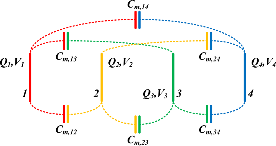
Motivated by that, this paper investigates possible coupling configurations of a four-plate CPT system and their system characteristics. Two of these four plates will serve as the primary power transmitter and the other two will be the secondary power receivers. The plates will be placed in parallel to each other with an equal distance. For instance, in Fig. 1, Plate 1 and Plate 2 can be used in the transmitting side, while Plate 3 and Plate 4 are on the receiving side. A mathematical model is established to describe the relationship among the plates in a 4 × 4 mutual capacitance matrix form. Each coupling configuration will be identified and analysed in detail and described in a general form. The electric field distributions of the coupling configurations will be simulated in ANSYS Maxwell. A practical CPT system will be built to verify theoretical modeling and analysis. To eliminate other factors (e.g. plate size, plate material, etc.) that may affect the results, four identical plates are used.
Block diagram of four parallelly and equidistantly placed identical metal plates.

The main contributions of this paper can be summarized as follows. The paper studies possible configurations and their corresponding system characteristics for a four-plate CPT system. It helps the researchers to gain a better understanding of the CPT power delivery mechanism. The findings can be used to predict the system performance in terms of load power, load voltage, and input impedance and to guide practical designs.
The rest of this paper is organized as follows: in “Mutual capacitance matrix of four parallely and equidistantly placed metal plates”, the mutual capacitance matrix is introduced to describe the CPT system with four parallelly and equidistantly placed metal plates. In “Coupling configurations under different connections of source and load”, mathematical expressions are derived in detail for different coupling configurations. Then a generalized expression is used to describe and predict the system performance. In “Electric field distribution analysis”, the electric field distribution analysis of the coupling configurations is presented. In “Experimental study”, a practical CPT system with four parallelly and equidistantly placed metal plates is established. With the numerical experiment results, it verifies the modeling of each coupling configuration. Finally, the conclusion is drawn in “Conclusion”.
2. Mutual capacitance matrix of four parallely and equidistantly placed metal plates
A four-plate CPT system can be simplified as four metal plates connecting with an AC voltage source and a load, regardless of the types of power converters and compensation networks used in a four-plate CPT system. The four plates can be arbitrarily placed in space. In this paper, four identical plates are placed parallelly to each other with the same spacing to simplify the following analysis and modeling.
In Fig. 1, the plates are labelled from left to right as Plate 1, Plate 2, Plate 3, and Plate 4. The quantity of electric charge on each plate is Q 1, Q 2, Q 3, and Q 4, respectively. The electric potential of each plate is V 1, V 2, V 3, and V 4. There would be six mutual capacitances existing in a four-plate CPT system, which are defined as C m,12, C m,13, C m,14, C m,23, C m,24, and C m,34, respectively. For example, C m,12 indicates how many charges on Plate 1 are contributed by the potential difference between Plates 1 and 2. The self-capacitance of each plate C m,11, C m,22, C m,33, and C m,44 is ignored in this paper because the distance between any two plates is much smaller than the distance between one plate and the reference at infinity.
Hence, the mutual capacitance matrix of these four parallelly and equidistantly placed identical metal plates can be described as follows:
 $$\left[ {\matrix{ {Q_1} \cr {Q_2} \cr {Q_3} \cr {Q_4} \cr}} \right] = \left[ {\matrix{ {C_{m,1}} & {-C_{m,12}} & {-C_{m,13}} & {-C_{m,14}} \cr {-C_{m,12}} & {C_{m,2}} & {-C_{m,23}} & {-C_{m,24}} \cr {-C_{m,13}} & {-C_{m,23}} & {C_{m,3}} & {-C_{m,34}} \cr {-C_{m,14}} & {-C_{m,24}} & {-C_{m,34}} & {C_{m,4}} \cr}} \right]\left[ {\matrix{ {V_1} \cr {V_2} \cr {V_3} \cr {V_4} \cr}} \right]$$
where
 $$\eqalign{C_{m,1} = &\;C_{m,11} + C_{m,12} + C_{m,13} + C_{m,14}\approx C_{m,12} + C_{m,13} + C_{m,14} \cr C_{m,2} = &\;C_{m,12} + C_{m,22} + C_{m,23} + C_{m,24}\approx C_{m,12} + C_{m,23} + C_{m,24} \cr C_{m,3} = &\;C_{m,13} + C_{m,23} + C_{m,33} + C_{m,34}\approx C_{m,13} + C_{m,23} + C_{m,34} \cr C_{m,4} = &\;C_{m,14} + C_{m,24} + C_{m,34} + C_{m,44}\approx C_{m,14} + C_{m,24} + C_{m,34}} $$
The above 4 × 4 matrix shows more degrees of freedom and technical possibilities for a four-plate CPT system. The voltage source can be applied between any two of the four plates, and the load can be connected to the other two plates. Accordingly, a four-plate CPT system will have different coupling configurations when different connections of voltage source and load are chosen.
It should be noted that this mathematical model is not limited to identical plates. These four plates can be of different sizes and be made of different materials. In practice, the plates on the receiving side can be more compact due to the space limitation. The mutual capacitance matrix equation is still valid regardless of the variations of plate sizes and plate materials. As this paper investigates different coupling configurations of a four-plate CPT system and their corresponding characteristics, the plates are assumed to be identical for a fair comparison.
3. Coupling configurations under different connections of source and load
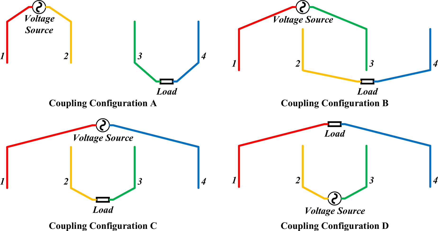
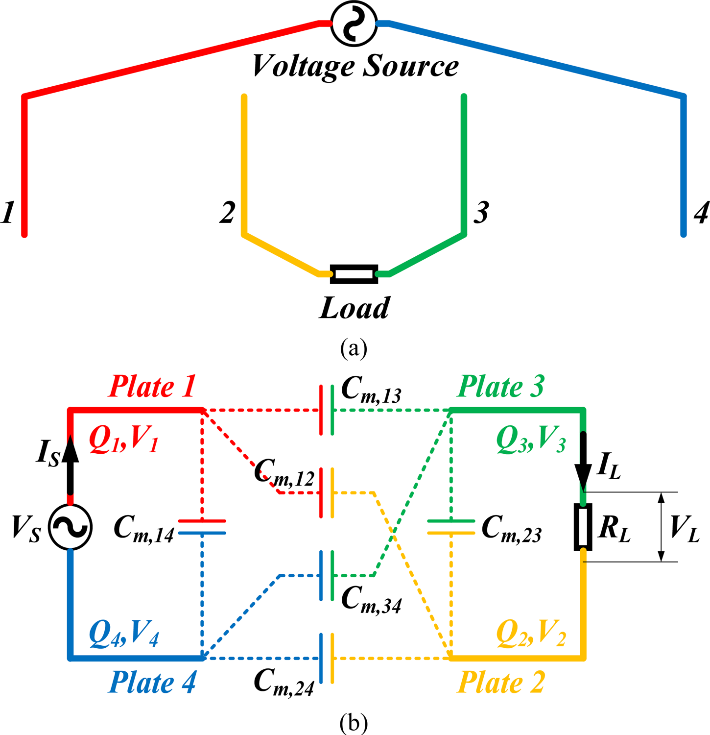
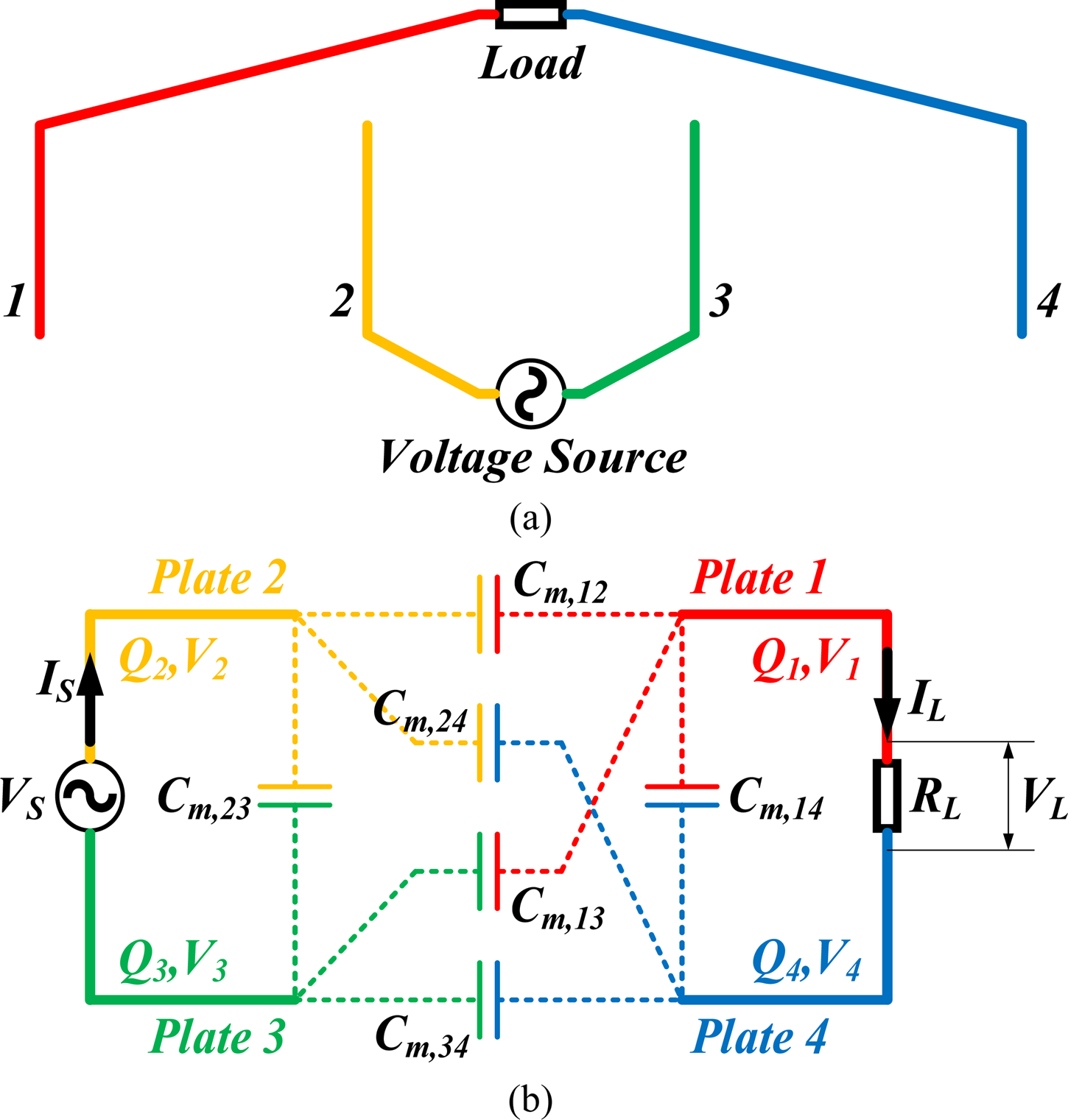
According to the geometry of four parallelly and equidistantly placed plates, there exists six different connections of the voltage source, the load, and four plates including (A) voltage source is connected between Plates 1 and 2, the load is between Plates 3 and 4; (B) voltage source is connected between Plates 1 and 3, load is between Plates 2 and 4; (C) voltage source is connected between Plates 1 and 4, load is between Plates 2 and 3; (D) voltage source is connected between Plates 2 and 3, load is between Plates 1 and 4; (E) voltage source is connected between Plates 2 and 4, load is between Plates 1 and 3; and (F) voltage source is connected between Plates 3 and 4, load is between Plates 1 and 2. Due to the symmetry of the mutual capacitance matrix of these four plates, (A) and (B) are the symmetric connections of (D) and (E). Hence, only (A), (B), (C), and (D) are analysed below in detail. In Fig. 2, an overview of these four possible coupling configurations is presented. In the following analysis, assume that the source voltage, current, and angular frequency are V S, I S, and ω, respectively, and the voltage and current of the load R L are V L and I L, respectively.
Overview of four possible coupling configurations.

3.1. Coupling configuration A: voltage source between Plates 1 and 2, load between Plates 3 and 4
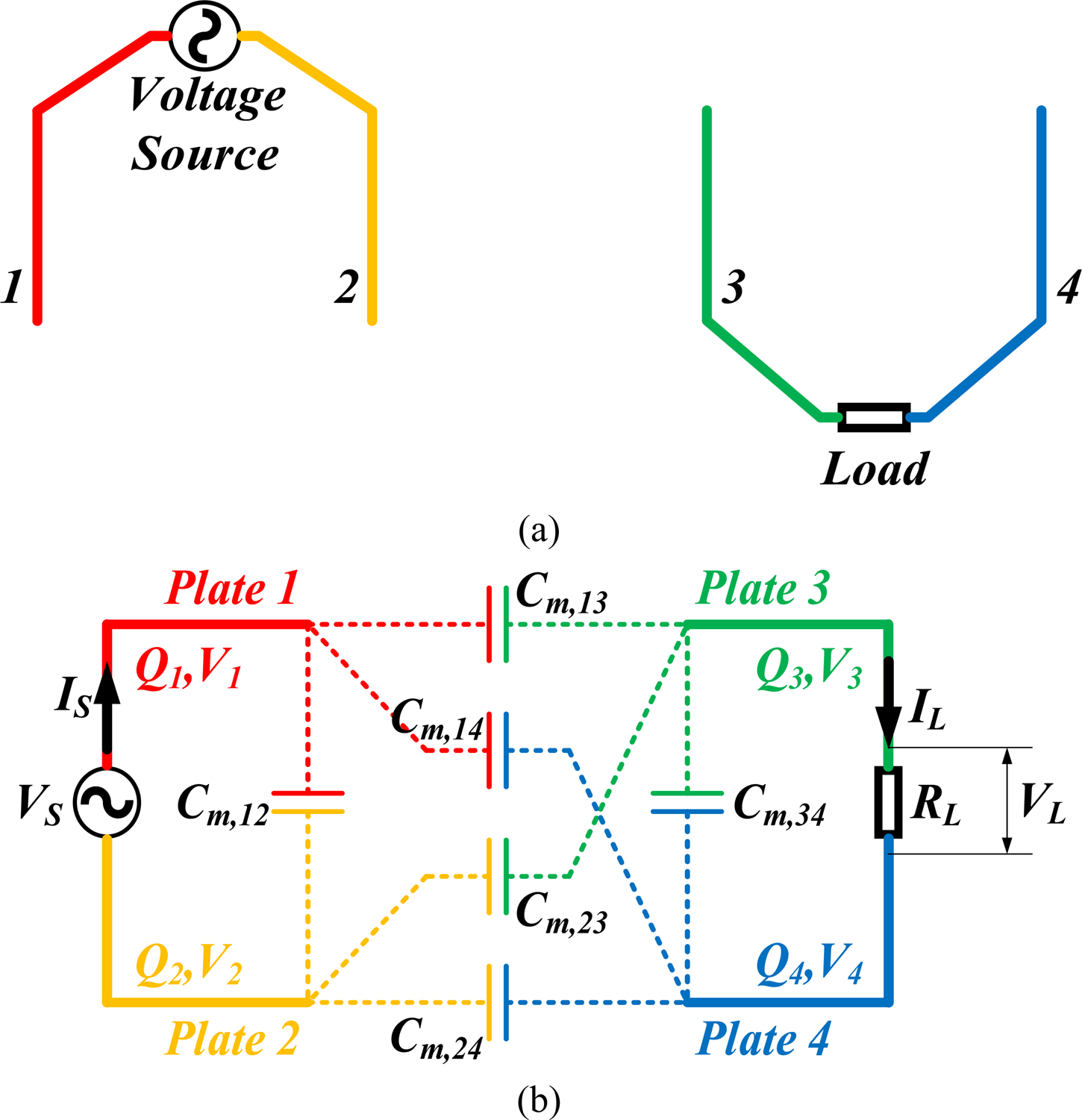
When the voltage source is applied between Plates 1 and 2 and the load is connected between Plates 3 and 4, the four-plate system transfers power by Coupling Configuration A as shown in Fig. 3.
(a) Physical connection and (b) equivalent circuit of Coupling Configuration A.

Let V 2 = 0, V s = V 1, V L = V 3 − V 4. According to Kirchhoff's current law, (1) can be reduced to the following matrix:
 $$\eqalign{\left[ {\matrix{ {Q_1} \cr {Q_2} \cr {Q_3} \cr {Q_4} \cr}} \right] & = \left[ {\matrix{ {I_S/j\omega} \cr {-I_S/j\omega} \cr {-I_L/j\omega} \cr {I_L/j\omega} \cr}} \right] \cr & = \left[ {\matrix{ {C_{m,1}} & {-C_{m,12}} & {-C_{m,13}} & {-C_{m,14}} \cr {-C_{m,12}} & {C_{m,2}} & {-C_{m,23}} & {-C_{m,24}} \cr {-C_{m,13}} & {-C_{m,23}} & {C_{m,3}} & {-C_{m,34}} \cr {-C_{m,14}} & {-C_{m,24}} & {-C_{m,34}} & {C_{m,4}} \cr}} \right]\left[ {\matrix{ {V_S} \cr 0 \cr {V_3} \cr {V_4} \cr}} \right]}$$
From the first two lines in (2), the relationship between V S, I S, and V L can be expressed as:
 $$\eqalign{ V_S &= \displaystyle{{I_S} \over {\,j\omega }} \cdot \displaystyle{{C_{m,13} + C_{m,14} + C_{m,23} + C_{m,24}} \over {C_{m,12}\left( {C_{m,13} + C_{m,14} + C_{m,23} + C_{m,24}} \right) + (C_{m,13} + C_{m,14})(C_{m,23} + C_{m,24})}} \cr & \quad + V_L\cdot \displaystyle{{C_{m,13}C_{m,24}-C_{m,14}C_{m,23}} \over {C_{m,12}\left( {C_{m,13} + C_{m,14} + C_{m,23} + C_{m,24}} \right) + (C_{m,13} + C_{m,14})(C_{m,23} + C_{m,24})}}} $$
Similarly, from the other two lines in (2), the relationship between V L, I L, and V S can be expressed as:
 $$ \eqalign{ V_L &= -\displaystyle{{I_L} \over {\,j\omega}} \cdot \displaystyle{{C_{m,13} + C_{m,14} + C_{m,23} + C_{m,24}} \over {C_{m,34}\lpar {C_{m,13} + C_{m,14} + C_{m,23} + C_{m,24}} \rpar + (C_{m,13} + C_{m,23})(C_{m,14} + C_{m,24})}} \cr & \quad + V_S\cdot \displaystyle{{C_{m,13}C_{m,24}-C_{m,14}C_{m,23}} \over {C_{m,34}\lpar {C_{m,13} + C_{m,14} + C_{m,23} + C_{m,24}} \rpar + (C_{m,13} + C_{m,23})(C_{m,14} + C_{m,24})}}} $$
(3) and (4) can be rewritten as:
 $$\left\{\eqalign{{I_S} & = {\,j\omega V_S\cdot \left[ {C_{m,12} + \displaystyle{{\left( {C_{m,13} + C_{m,14}} \right)\left( {C_{m,23} + C_{m,24}} \right)} \over {C_{m,13} + C_{m,14} + C_{m,23} + C_{m,24}}}} \right]} \cr & \quad-{\,j\omega V_L\cdot \displaystyle{{C_{m,13}C_{m,24}-C_{m,14}C_{m,23}} \over {C_{m,13} + C_{m,14} + C_{m,23} + C_{m,24}}}} \cr & {I_L} = j\omega V_S\cdot \displaystyle{{C_{m,13}C_{m,24}-C_{m,14}C_{m,23}} \over {C_{m,13} + C_{m,14} + C_{m,23} + C_{m,24}}} \cr &\quad -{\,j\omega V_L\cdot \left[ {C_{m,34} + \displaystyle{{\left( {C_{m,13} + C_{m,23}} \right)\left( {C_{m,14} + C_{m,24}} \right)} \over {C_{m,13} + C_{m,14} + C_{m,23} + C_{m,24}}}} \right]}}\right.$$
Because I L = V L/R L, the input impedance from the source side can be derived from the first equation of (5):
 $$Z_{in} = \displaystyle{1 \over \matrix{\,j\omega \left[ {C_{m,12} + \displaystyle{{\left( {C_{m,13} + C_{m,14}} \right)\left( {C_{m,23} + C_{m,24}} \right)} \over {C_{m,13} + C_{m,14} + C_{m,23} + C_{m,24}}}} \right] + \hfill \cr \displaystyle{{\omega ^2{\left( {\displaystyle{{C_{m,13}C_{m,24}-C_{m,14}C_{m,23}} \over {C_{m,13} + C_{m,14} + C_{m,23} + C_{m,24}}}} \right)}^2} \over {\displaystyle{1 \over {R_L}} + j\omega \left[ {C_{m,34} + \displaystyle{{\left( {C_{m,13} + C_{m,23}} \right)\left( {C_{m,14} + C_{m,24}} \right)} \over {C_{m,13} + C_{m,14} + C_{m,23} + C_{m,24}}}} \right]}} \hfill} }$$
The load voltage can be derived from the second equation of (5):
 $$V_L = \displaystyle{{\,j\omega \displaystyle{{C_{m,13}C_{m,24}-C_{m,14}C_{m,23}} \over {C_{m,13} + C_{m,14} + C_{m,23} + C_{m,24}}}} \over {\displaystyle{1 \over {R_L}} + j\omega \left[ {C_{m,34} + \displaystyle{{\lpar {C_{m,13} + C_{m,23}} \rpar \lpar {C_{m,14} + C_{m,24}} \rpar } \over {C_{m,13} + C_{m,14} + C_{m,23} + C_{m,24}}}} \right]}}V_S$$
Hence, the load power can be expressed as:
 $$P_L = \displaystyle{{\omega ^2{\left( {\displaystyle{{C_{m,13}C_{m,24}-C_{m,14}C_{m,23}} \over {C_{m,13} + C_{m,14} + C_{m,23} + C_{m,24}}}} \right)}^2} \over {{\left( {\displaystyle{1 \over {R_L}}} \right)}^2 + \omega ^2{\left[ {C_{m,34} + \displaystyle{{\lpar {C_{m,13} + C_{m,23}} \rpar \lpar {C_{m,14} + C_{m,24}} \rpar } \over {C_{m,13} + C_{m,14} + C_{m,23} + C_{m,24}}}} \right]}^2}} \cdot \displaystyle{{{\vert {V_S} \vert } ^2} \over {R_L}}$$
3.2. Coupling configuration B: voltage source between Plates 1 and 3, load between Plates 2 and 4
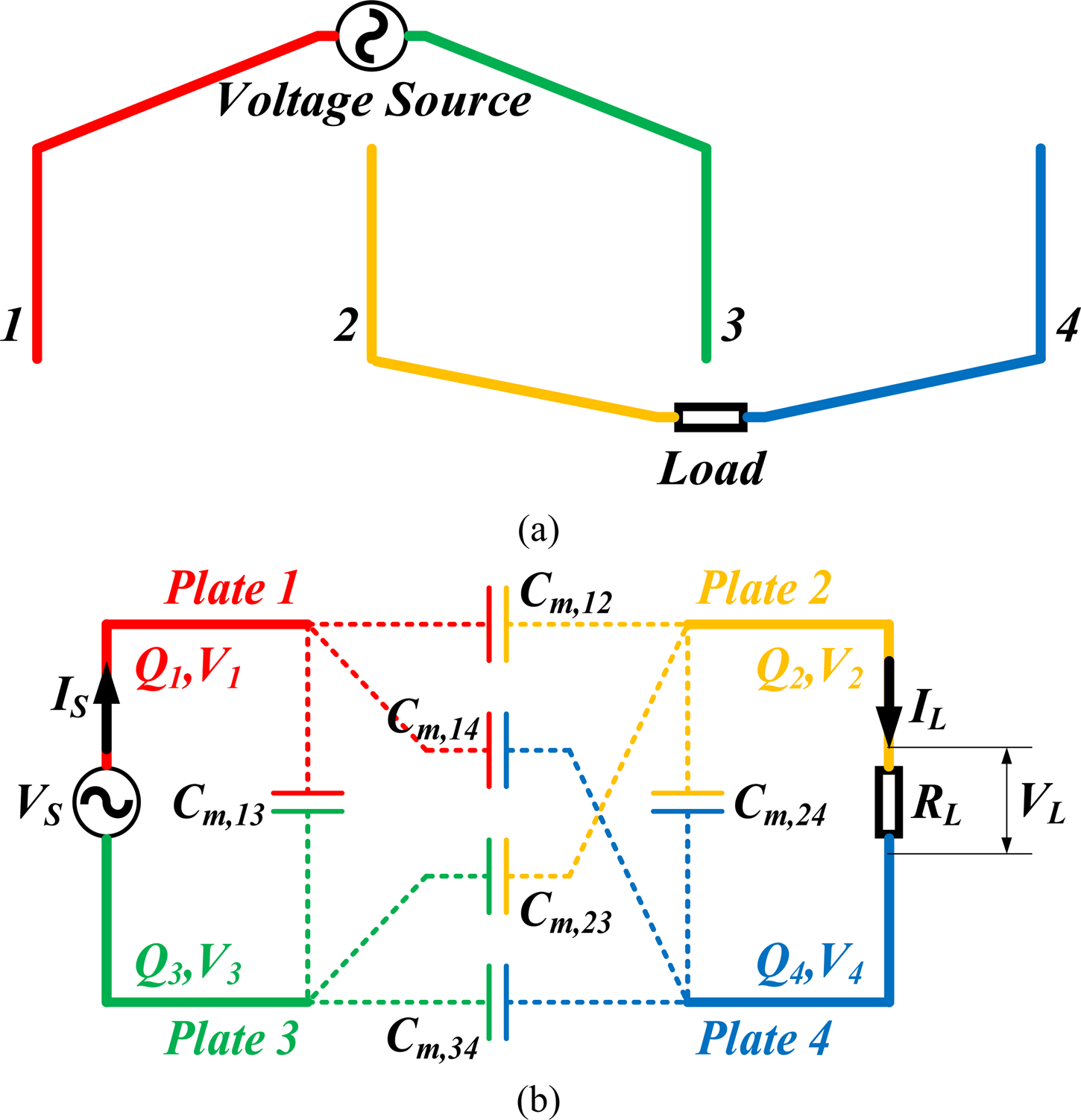
When the voltage source is applied between Plates 1 and 3 and the load is connected between Plates 2 and 4, the four-plate system transfers power by Coupling Configuration B as shown in Fig. 4.
(a) Physical connection and (b) equivalent circuit of Coupling Configuration B.

Similar to the analysis conducted in Coupling Configuration A, the input impedance from the source side in Coupling Configuration B can be expressed as:
 $$Z_{in} = \displaystyle{1 \over \matrix{\,j\omega \left[ {C_{m,13} + \displaystyle{{\left( {C_{m,12} + C_{m,14}} \right)\left( {C_{m,23} + C_{m,34}} \right)} \over {C_{m,12} + C_{m,14} + C_{m,23} + C_{m,34}}}} \right] \hfill \cr + \displaystyle{{\omega ^2{\left( {\displaystyle{{C_{m,12}C_{m,34}-C_{m,14}C_{m,23}} \over {C_{m,12} + C_{m,14} + C_{m,23} + C_{m,34}}}} \right)}^2} \over {\displaystyle{1 \over {R_L}} + j\omega \left[ {C_{m,24} + \displaystyle{{\left( {C_{m,12} + C_{m,23}} \right)\left( {C_{m,14} + C_{m,34}} \right)} \over {C_{m,12} + C_{m,14} + C_{m,23} + C_{m,34}}}} \right]}} \hfill} }$$
The load voltage in Coupling Configuration B can be expressed as:
 $$V_L = \displaystyle{{\,j\omega \displaystyle{{C_{m,12}C_{m,34}-C_{m,14}C_{m,23}} \over {C_{m,12} + C_{m,14} + C_{m,23} + C_{m,34}}}} \over {\displaystyle{1 \over {R_L}} + j\omega \left[ {C_{m,24} + \displaystyle{{\lpar {C_{m,12} + C_{m,23}} \rpar \lpar {C_{m,14} + C_{m,34}} \rpar } \over {C_{m,12} + C_{m,14} + C_{m,23} + C_{m,34}}}} \right]}}V_S$$
The load power in Coupling Configuration B can be expressed as:
 $$\eqalign{P_L & = \displaystyle{{\omega ^2{\left( {\displaystyle{{C_{m,12}C_{m,34}-C_{m,14}C_{m,23}} \over {C_{m,12} + C_{m,14} + C_{m,23} + C_{m,34}}}} \right)}^2} \over {{\left( {\displaystyle{1 \over {R_L}}} \right)}^2 + \omega ^2{\left[ {C_{m,24} + \displaystyle{{\lpar {C_{m,12} + C_{m,23}} \rpar \lpar {C_{m,14} + C_{m,34}} \rpar } \over {C_{m,12} + C_{m,14} + C_{m,23} + C_{m,34}}}} \right]}^2}} \cr & \quad \cdot \displaystyle{{{\vert {V_S} \vert } ^2} \over {R_L}}}$$
3.3. Coupling configuration C: voltage source between Plates 1 and 4, load between Plates 2 and 3
When the voltage source is applied between Plates 1 and 4 and the load is connected between Plates 2 and 3, the four-plate system transfers power by Coupling Configuration C as shown in Fig. 5.
(a) Physical connection and (b) equivalent circuit of Coupling Configuration C.

Similar to the analysis conducted in Coupling Configuration A, the input impedance from the source side in Coupling Configuration C can be expressed as:
 $$Z_{in} = \displaystyle{1 \over \matrix{\,j\omega \left[ {C_{m,14} + \displaystyle{{\left( {C_{m,12} + C_{m,13}} \right)\left( {C_{m,24} + C_{m,34}} \right)} \over {C_{m,12} + C_{m,13} + C_{m,24} + C_{m,34}}}} \right] \hfill \cr + \displaystyle{{\omega ^2{\left( {\displaystyle{{C_{m,13}C_{m,24}-C_{m,12}C_{m,34}} \over {C_{m,12} + C_{m,13} + C_{m,24} + C_{m,34}}}} \right)}^2} \over {\displaystyle{1 \over {R_L}} + j\omega \left[ {C_{m,23} + \displaystyle{{\left( {C_{m,12} + C_{m,24}} \right)\left( {C_{m,13} + C_{m,34}} \right)} \over {C_{m,12} + C_{m,13} + C_{m,24} + C_{m,34}}}} \right]}} \hfill} }$$
The load voltage in Coupling Configuration C can be expressed as:
 $$V_L = \displaystyle{{\,j\omega \displaystyle{{C_{m,13}C_{m,24}-C_{m,12}C_{m,34}} \over {C_{m,12} + C_{m,13} + C_{m,24} + C_{m,34}}}} \over {\displaystyle{1 \over {R_L}} + j\omega \left[ {C_{m,23} + \displaystyle{{\lpar {C_{m,12} + C_{m,24}} \rpar \lpar {C_{m,13} + C_{m,34}} \rpar } \over {C_{m,12} + C_{m,13} + C_{m,24} + C_{m,34}}}} \right]}}V_S$$
The load power in Coupling Configuration C can be expressed as:
 $$\eqalign{P_L &= \displaystyle{{\omega ^2{\left( {\displaystyle{{C_{m,13}C_{m,24}-C_{m,12}C_{m,34}} \over {C_{m,12} + C_{m,13} + C_{m,24} + C_{m,34}}}} \right)}^2} \over {{\left( {\displaystyle{1 \over {R_L}}} \right)}^2 + \omega ^2{\left[ {C_{m,23} + \displaystyle{{\lpar {C_{m,12} + C_{m,24}} \rpar \lpar {C_{m,13} + C_{m,34}} \rpar } \over {C_{m,12} + C_{m,13} + C_{m,24} + C_{m,34}}}} \right]}^2}} \cr &\quad \cdot\displaystyle{{{\vert {V_S} \vert } ^2} \over {R_L}}}$$
3.4. Coupling configuration D: voltage source between Plates 2 and 3, load between Plates 1 and 4
When the voltage source is applied between Plates 2 and 3 and the load is connected between Plates 1 and 4, the four-plate system transfers power by Coupling Configuration D as shown in Fig. 6.
(a) Physical connection and (b) equivalent circuit of Coupling Configuration D.

Similar to the analysis conducted in Coupling Configuration A, the input impedance from the source side in Coupling Configuration D can be expressed as:
 $$Z_{in} = \displaystyle{1 \over \matrix{\,j\omega \left[ {C_{m,23} + \displaystyle{{\left( {C_{m,12} + C_{m,24}} \right)\left( {C_{m,13} + C_{m,34}} \right)} \over {C_{m,12} + C_{m,13} + C_{m,24} + C_{m,34}}}} \right] \hfill \cr + \displaystyle{{\omega ^2{\left( {\displaystyle{{C_{m,12}C_{m,34}-C_{m,13}C_{m,24}} \over {C_{m,12} + C_{m,13} + C_{m,24} + C_{m,34}}}} \right)}^2} \over {\displaystyle{1 \over {R_L}} + j\omega \left[ {C_{m,14} + \displaystyle{{\left( {C_{m,12} + C_{m,13}} \right)\left( {C_{m,24} + C_{m,34}} \right)} \over {C_{m,12} + C_{m,13} + C_{m,24} + C_{m,34}}}} \right]}} \hfill} }$$
The load voltage in Coupling Configuration D can be expressed as:
 $$V_L = \displaystyle{{\,j\omega \displaystyle{{C_{m,12}C_{m,34}-C_{m,13}C_{m,24}} \over {C_{m,12} + C_{m,13} + C_{m,24} + C_{m,34}}}} \over {\displaystyle{1 \over {R_L}} + j\omega \left[ {C_{m,14} + \displaystyle{{\lpar {C_{m,12} + C_{m,13}} \rpar \lpar {C_{m,24} + C_{m,34}} \rpar } \over {C_{m,12} + C_{m,13} + C_{m,24} + C_{m,34}}}} \right]}}V_S$$
The load power in Coupling Configuration D can be expressed as:
 $$\eqalign{P_L & = \displaystyle{{\omega ^2{\left( {\displaystyle{{C_{m,12}C_{m,34}-C_{m,13}C_{m,24}} \over {C_{m,12} + C_{m,13} + C_{m,24} + C_{m,34}}}} \right)}^2} \over {{\left( {\displaystyle{1 \over {R_L}}} \right)}^2 + \omega ^2{\left[ {C_{m,14} + \displaystyle{{\lpar {C_{m,12} + C_{m,13}} \rpar \lpar {C_{m,24} + C_{m,34}} \rpar } \over {C_{m,12} + C_{m,13} + C_{m,24} + C_{m,34}}}} \right]}^2}}\cr & \cdot \displaystyle{{{\vert {V_S} \vert } ^2} \over {R_L}}}$$
3.5. Generalized description of different coupling configurations and mutual capacitance calculation
Once four plates have been placed, the mutual capacitances C m,12, C m,13, C m,14, C m,23, C m,24, and C m,34 are assumed constant. With the above mathematical analysis, the researchers can easily obtain the corresponding input impedance, the load voltage, and the load power of a four-plate system given any of these four coupling configurations in “Coupling configuration A: voltage source between plates 1 and 2, load between plates 3 and 4”, “Coupling configuration B: voltage source between Plates 1 and 3, load between Plates 2 and 4”, “Coupling configuration C: voltage source between Plates 1 and 4, load between Plates 2 and 3”, and “Coupling configuration D: voltage source between Plates 2 and 3, load between Plates 1 and 4”. Then a generalized mathematical description is summarized and explains the mechanism of power delivery in CPT.
Assume that the voltage source is applied between the plates i and j, and the load is connected to the plates k and l, where 1≤i, j, k, l≤4 and they are not equal to each other. Hence, the input impedance, load voltage, and load power of this four-plate system can be expressed as follows:
 $$Z_{in} = \displaystyle{1 \over {\,j\omega C_1 + (\omega ^2C_M^2 /((1/R_L) + j\omega C_2))}}$$
 $$V_L = \displaystyle{{\,j\omega C_M} \over {((1/R_L) + j\omega C_2)}}V_S$$
 $$P_L = \displaystyle{{\omega ^2C_M^2} \over {({(1/R_L)}^2 + \omega ^2C_2^2 )}}\cdot \displaystyle{{{\vert {V_S} \vert } ^2} \over {R_L}}$$
where,
 $$\eqalign{C_1 =\; &C_{m,ij} + \displaystyle{{\lpar {C_{m,ik} + C_{m,il}} \rpar \lpar {C_{m,jk} + C_{m,jl}} \rpar } \over {C_{m,ik} + C_{m,il} + C_{m,jk} + C_{m,jl}}} \cr C_2 =\; &C_{m,kl} + \displaystyle{{\lpar {C_{m,ik} + C_{m,jk}} \rpar \lpar {C_{m,il} + C_{m,jl}} \rpar } \over {C_{m,ik} + C_{m,il} + C_{m,jk} + C_{m,jl}}} \cr C_M =\; &\displaystyle{{C_{m,ik}C_{m,jl}-C_{m,il}C_{m,jk}} \over {C_{m,ik} + C_{m,il} + C_{m,jk} + C_{m,jl}}}} $$
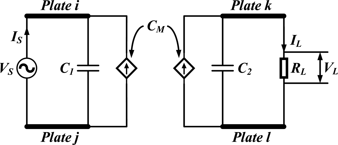
From (18)–(20), the equivalent circuit of the studied four-plate system is shown in Fig. 7. Based on (19) and (20), once the source voltage including amplitude and frequency is determined, power can be transferred by the mutual capacitance between the transmitter and receiver plates C ik, C il, C jk, C jl. The transferred power is also decided by the capacitance between the two receiver plates C kl and the load resistance R L.
The equivalent circuit of the studied four-plate CPT System.

Due to the symmetry of the placement of four plates, let C x = C m,12 = C m,23 = C m,34, C y = C m,13 = C m,24, and C z = C m,14. When no load is connected, the total capacitance between arbitrary two plates can be express as follows based on (6), (9), (12), and (15).
 $$\eqalign{C_{total,12} & = C_x + \displaystyle{{\lpar {C_y + C_z} \rpar \lpar {C_x + C_y} \rpar } \over {C_x + 2C_y + C_z}} \cr & -\displaystyle{{{\left( {\displaystyle{{C_yC_y-C_xC_z} \over {C_x + 2C_y + C_z}}} \right)}^2} \over {C_x + \displaystyle{{\lpar {C_x + C_y} \rpar \lpar {C_y + C_z} \rpar } \over {C_x + 2C_y + C_z}}}}}$$
 $$\eqalign{C_{total,13} & = C_y + \displaystyle{{\lpar {C_x + C_z} \rpar \lpar {C_x + C_x} \rpar } \over {3C_x + C_z}} \cr & -\displaystyle{{{\left( {\displaystyle{{C_xC_x-C_xC_z} \over {3C_x + C_z}}} \right)}^2} \over {C_y + \displaystyle{{\lpar {C_x + C_x} \rpar \lpar {C_x + C_z} \rpar } \over {3C_x + C_z}}}}}$$
 $$\eqalign{C_{total,14} & = C_z + \displaystyle{{\lpar {C_x + C_y} \rpar \lpar {C_x + C_y} \rpar } \over {2C_x + 2C_y}}- \cr & \displaystyle{{{\left( {\displaystyle{{C_yC_y-C_xC_x} \over {2C_x + 2C_y}}} \right)}^2} \over {C_x + \displaystyle{{\lpar {C_x + C_y} \rpar \lpar {C_x + C_y} \rpar } \over {2C_x + 2C_y}}}}}$$
 $$\eqalign{C_{total,23} & = C_x + \displaystyle{{\lpar {C_x + C_y} \rpar \lpar {C_x + C_y} \rpar } \over {2C_x + 2C_y}} \cr & -\displaystyle{{{\left( {\displaystyle{{C_xC_x-C_yC_y} \over {2C_x + 2C_y}}} \right)}^2} \over {C_z + \displaystyle{{\lpar {C_x + C_y} \rpar \lpar {C_x + C_y} \rpar } \over {2C_x + 2C_y}}}}}$$
where C total,12, C total,13, C total,14, and C total,23 mean the total capacitance between the Plates 1 and 2, Plates 1 and 3, Plates 1 and 4, and Plates 2 and 3, respectively. Once the placement of four plates is determined, according to (21)–(24), there are four equations for solving three unknown variables C x, C y, and C z.
It should be noted that equations (21)–(24) are based on the placement of four identical parallelly placed metal plates with the same spacing. If the placement of four plates is asymmetrical or the plates are not identical, six total capacitances C total,12, C total,13, C total,14, C total,23, C total,24, and C total,34 can be obtained by measuring the total capacitance between any two plates. Based on these six total capacitances, C m,12, C m,23, C m,34, C m,23, C m,34, and C m,34 can be respectively solved. The solving process of six mutual capacitances can be easily realized by mathematical calculation software.
4. Electric field distribution analysis
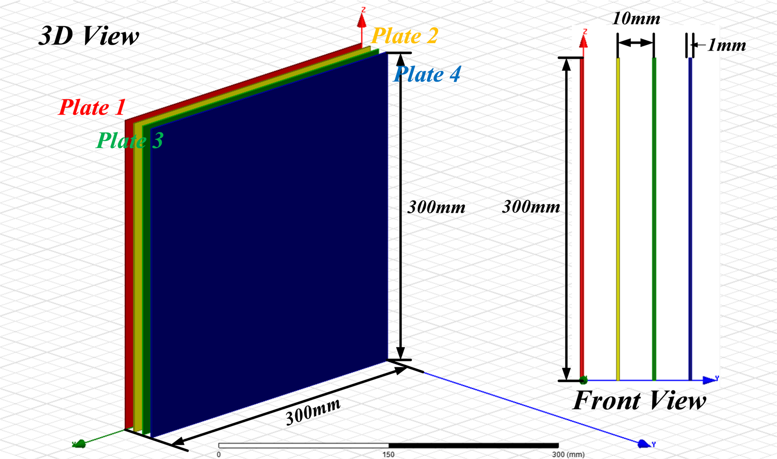
This section will analyse the four-plate CPT system from the angle of the electric field distribution and use the software ANSYS Maxwell to show the electric field coupling among four plates when any two of the four plates are excited by a voltage source and no load is connected to the other two plates. A simulation model consisting of four vertically placed 300 mm × 300 mm square aluminum plates with 10 mm spacing and 1 mm thickness is built as shown in Fig. 8. Four plates are marked red, yellow, green, and blue, representing Plate 1, Plate 2, Plate 3, and Plate 4, respectively. The source voltage is set to be 50 Vrms@1 MHz.
Configuration consisting of four parallelly placed 300 mm × 300 mm square aluminum plates with 10 mm spacing and 1 mm thickness.

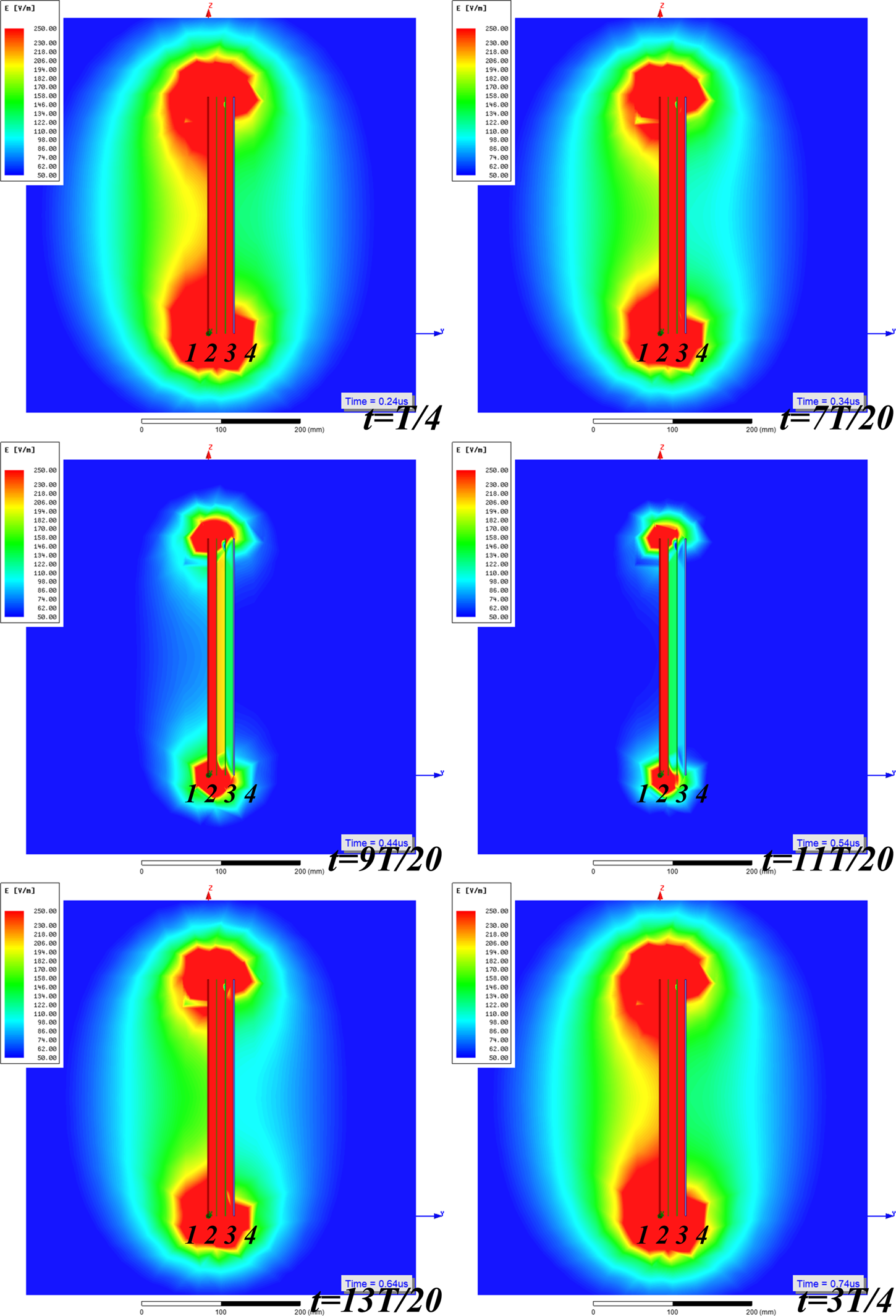
Figure 9 shows the electric field distribution of Coupling Configuration A at different instants of a period, where the source voltage is connected between Plate 1 and Plate 2, and T = 1 µs.
Electric field distribution of Coupling Configuration A at different instants of a period.

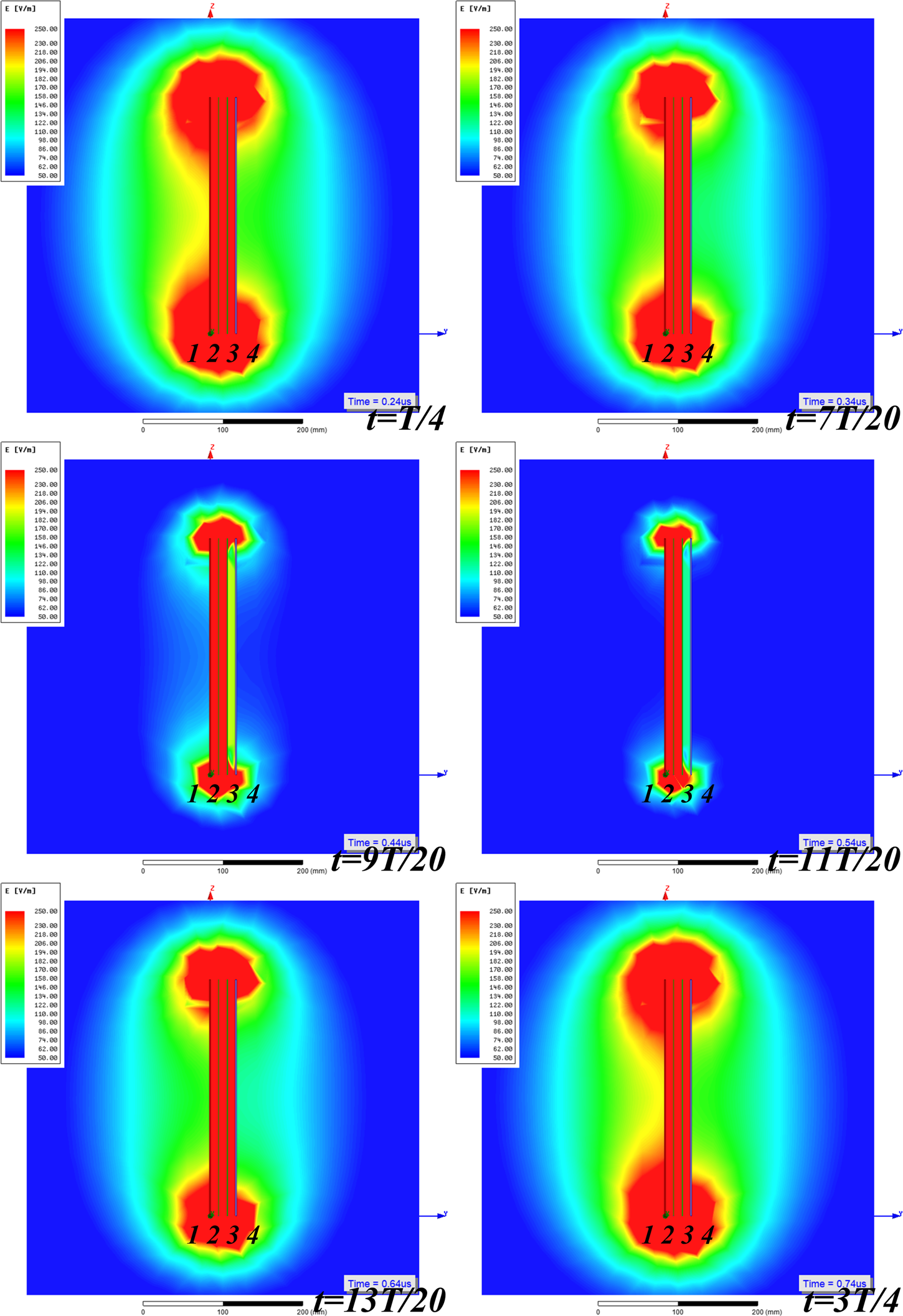
Figure 10 shows the electric field distribution of Coupling Configuration B at different instants of a period, where the source voltage is connected between Plate 1 and Plate 3, and T = 1 µs.
Electric field distribution of Coupling Configuration B at different instants of a period.

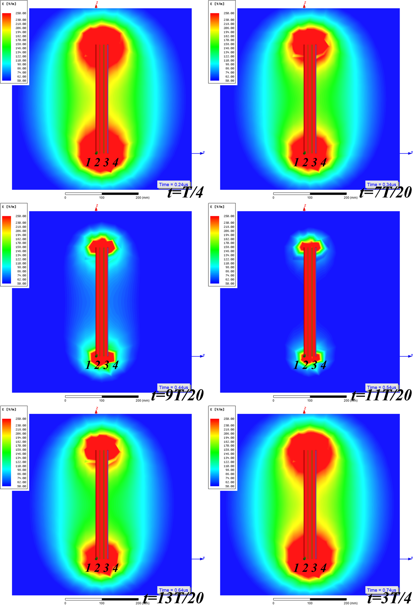
Figure 11 shows the electric field distribution of Coupling Configuration C at different instants of a period, where the source voltage is connected between Plate 1 and Plate 4, and T = 1 µs.
Electric field distribution of Coupling Configuration C at different instants of a period.

Figure 12 shows the electric field distribution of Coupling Configuration D at different instants of a period, where the source voltage is connected between Plate 2 and Plate 3, and T = 1 µs.
Electric field distribution of Coupling Configuration D at different instants of a period.

From Figures 9–12, the results show that complex electric field couplings always exist among four plates regardless of different connection methods. Power can be transferred via these complex electric field couplings. Once the placement of four plates is determined, the mutual capacitance matrix will be constructed and the electric field couplings among four plates under the excitation of the voltage source can be predicted.
From the electric field distribution at the instant t = 9 T/20 or t = 11 T/20 in four coupling configurations, there is a strong electric coupling between the two source plates even when the voltage applied between these two plates is almost zero. The maximum strength of electric coupling or the maximum potential difference occurs at the instant t = T/4 or t = 3 T/4. The strength of this electric coupling varies with time, which will cause a time-varying potential difference between the other two plates.
In this study, it is found that Configuration D has less leakage electric fields than other configurations at all instants. The leakage electric fields in Coupling Configurations A and B are asymmetrical because of the asymmetry of the two source plates. The range of the leakage electric field in Coupling Configuration A is slightly larger than that of Coupling Configuration B. Meanwhile, the leakage electric fields in Coupling Configurations C and D are dumbbell-shaped and symmetrical. The range of the leakage electric field in Coupling Configuration C is obviously larger than that of Coupling Configuration D. The placement of the two non-source plates will affect the electric field distribution even when the source voltage is kept unchanged. This can be useful for designing an electric coupler with a low-leakage electric field in a CPT system.
5. Experimental study
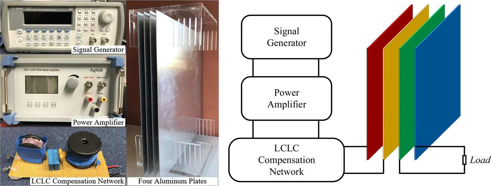
A four-plate CPT system is shown in Fig. 13. The setup composes of a signal generator Agilent 33220A for generating a high-frequency voltage, a wideband power amplifier Agitek ATA-122D for amplifying the output voltage of the signal generator, an LCLC compensation network for further boosting the output voltage of power amplifier, four parallelly placed 300 mm × 300 mm square aluminum plates with 10 mm spacing and 1 mm thickness, and some different loads. In the experiments, two plates are connected to the output of the LCLC compensation network, and the other two plates are connected to the resistor. The voltage applied between two plates is set to be 50 Vrms@1 MHz. It should be noted that the signal generator and the power amplifier are powered by an isolation transformer to avoid connecting any plate directly to the ground, and a battery-powered handheld oscilloscope Keysight U1620A is used in the experiments to reduce the effect of the ground on the measurement results.
A practical CPT system with four parallelly and equidistantly placed metal plates.

The placement of four plates is shown in Fig. 13, hence, the mutual capacitance matrix can be expressed as follows:
 $$C = \left[ {\matrix{ {87.12} & {-84.79} & {-1.04} & {-1.29} \cr {-84.79} & {170.62} & {-84.79} & {-1.04} \cr {-1.04} & {-84.79} & {170.62} & {-84.79} \cr {-1.29} & {-1.04} & {-84.79} & {87.12} \cr}} \right]{\rm pF}$$
It should be noticed that it is not easy to directly measure the mutual capacitance between any two plates when the placement of four plates is determined. However, the mutual capacitance can be obtained by two indirect measurement methods. One method is to set up an identical structure of four plates in the simulation software and calculate the mutual capacitance matrix based on the simulation model. The other method is to measure the total impedance between any two of the four plates by the RLC meter and solve the value of each mutual capacitance by equations (21), (22), (23), and (24). In this paper, the second method is taken to obtain the mutual capacitance between any two plates. C total,12 = 87.04 pF, C total,13 = 44.95 pF, C total,14 = 30.48 pF, hence, C x = 84.79 pF, C y = 1.04 pF, and C z = 1.29 pF. Meanwhile, the placement of these four plates is modeled in Ansys Maxwell, and C m,1 = 89.36 pF, C m,2 = 173.92 pF, C m,3 = 174.45 pF, C m,4 = 91.83 pF, C m,12 = 86.17 pF, C m,13 = 1.36 pF, C m,14 = 1.83 pF, C m,23 = 85.42 pF, C m,24 = 2.33 pF, and C m,34 = 87.67 pF. Considering the difference between the actual plates used in the experiments and the modeled plates in the simulation software, the results of both methods are in good agreement.
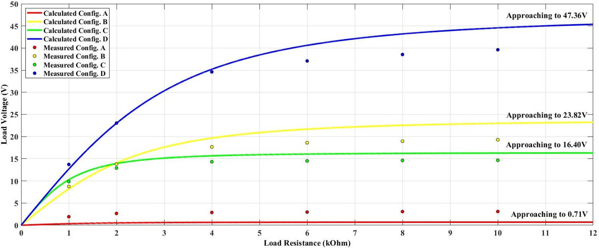
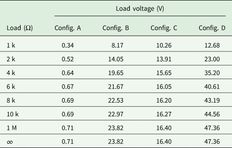
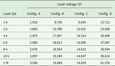
The excitation voltage applied between two source plates is set to 50 Vrms@1 MHz in simulations and experiments. By substituting (25) into (7), (10), (13), and (16), the calculated voltage of the load under different load conditions in Coupling Configurations A, B, C, and D can be obtained, as shown in Table 1. The experiment values of the load voltages are collected in Table 2. The curves of the calculated and measured load voltage against load resistance are then plotted for all configurations in Fig. 14.
Curves of the calculated and measured load voltage against load resistance in four coupling configurations.

Calculated voltage of the load under different load conditions in different coupling configurations

Measured voltage of the load under different load conditions in different coupling configurations

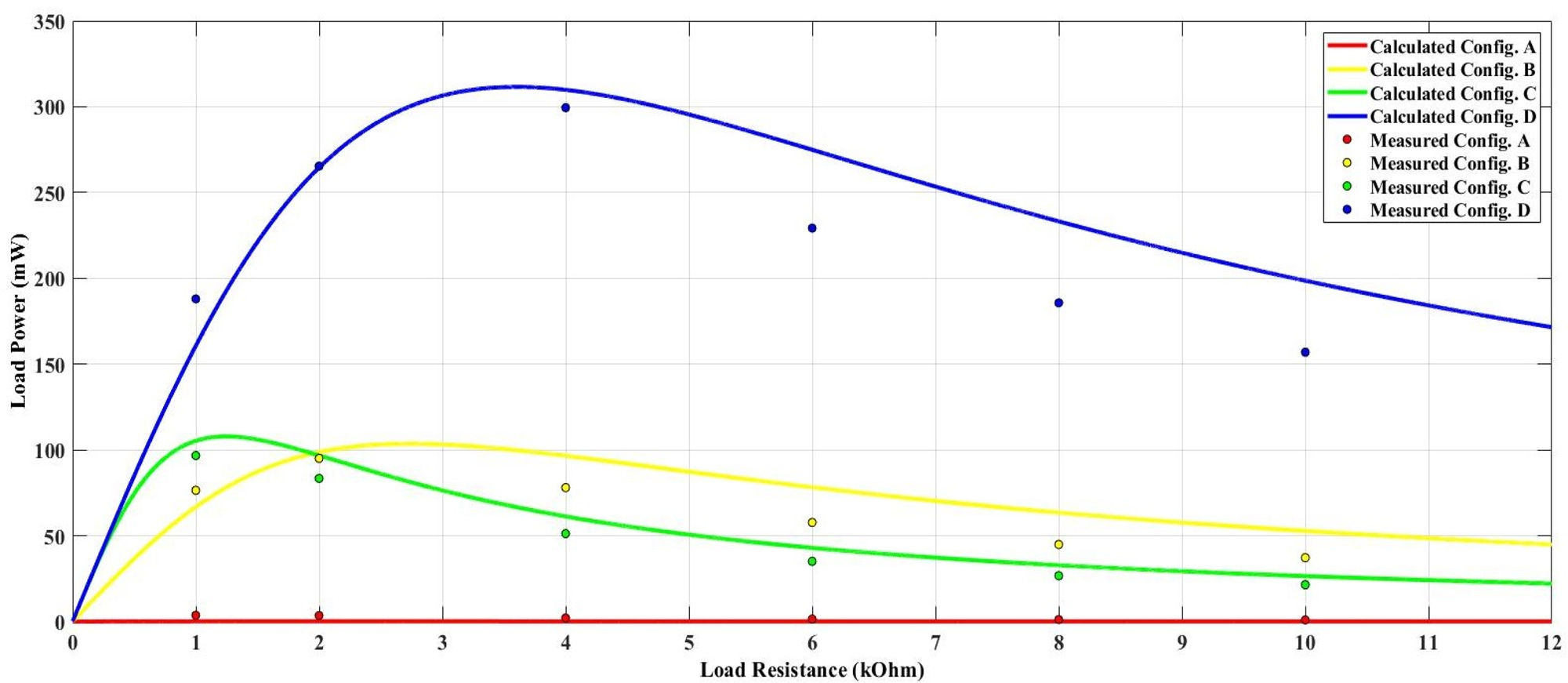
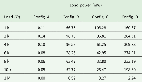
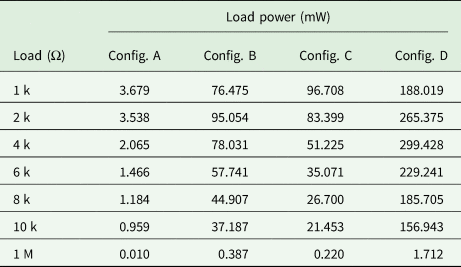
Similarly, by substituting (25) into (8), (11), (14), and (17), the calculated power of the load under different load conditions in Coupling Configurations A, B, C and D can be obtained, as shown in Table 3. Table 4 shows the load power obtained by the measured load voltage under different load conditions. The curves of the calculated and measured load power against load resistance in four coupling configurations are shown in Fig. 15.
Curves of the calculated and measured load power against load resistance in four coupling configurations.

Calculated power of the load under different load conditions in different coupling configurations

Load power obtained by the measured load voltage under different load conditions in different coupling configurations

From the data obtained above, it could be found that Configuration D has the highest load voltage as well as the load power in this setup. However, Configuration A, the most commonly used configuration, has the lowest load voltage and load power. When the load resistance is smaller than 2 kΩ, Configuration C has a higher load voltage and load power. However, the load voltage in Configuration B is larger than that in Configuration C when the load resistance is larger than 2 kΩ.
The discrepancy between theoretical and actual values can be caused by many factors. As the experiment is conducted under 1 MHz, the results can be easily affected by the surroundings and experiment equipment. For example, the probes can bring in external capacitance to the system when conducting measurements. Even with the differential probes, the small capacitance introduced can change the original capacitance matrix. Other factors like connection cables, plate misalignment, plate quality, etc. can also affect accuracy. In the case of Configuration A, the load voltage and power are inherently small, and the relative error caused by the mutual capacitance variations is even larger than them. For example, the voltage across a 1 MΩ resistor of Configuration A increases to 2.5 V when the values of C m,13, C m,24, and C m,14 in (25) are just increased by 5 pF. These voltage variations will be squared and cause higher load power variations.
In practise, Configuration A is most commonly used for its flexibility and freedom. However, in this study, it could be found that Configuration A has the lowest power transfer density. When the application has limited space and fixed plate distance (e.g. synchronous machines [Reference Ludois, Reed and Hanson8–Reference Ludois and Reed10], rotary CPT system [Reference Liu, Hu and Nair27, Reference Zang, Lu, Nguang and Sun28]), Configuration D can be applied to transfer maximum power.
6. Conclusion
In this paper, it studies possible coupling configurations of a four-plate CPT system. By changing the connections of the source and load, the four-plate CPT can have different power transfer capabilities and electric field distribution. A mathematical model based on a 4 × 4 mutual capacitance matrix for a simplified placement of four parallelly and equidistantly placed metal plates has been established. Four different coupling configurations have been identified and analysed in detail and described in a general form. The electric field distributions of the coupling configurations have been simulated in ANSYS Maxwell. A practical system consisting of four parallelly placed 300 mm × 300 mm aluminum plates with 10 mm spacing, a 50 Vrms@1 MHz voltage source, and different loads has been built. The experimental results have shown that the measured output voltage and power under the four coupling configurations are in good agreement with the theoretical results. It has found that the voltage gain is the highest when the two inner plates are chosen as the primary power transmitters, and this coupling configuration also has the lowest leakage electric field. The findings from this paper can be used to guide the design of four-plate CPT systems in some specific scenarios.
Acknowledgement
This work was supported in part by Hunan Provincial Science and Technology Department under Grant 2018TP1001, in part by the National Key R&D Program of China under Grant 2018YFB0606005, and in part by the China Scholarship Council under Grant 201706370068.
 Qi Zhu was born in Anhui Province, China, in 1993. He received the B.S. degree in electrical engineering and automation from Central South University, Changsha, China, in 2014, where he is currently working toward the Ph.D. degree in electrical engineering. From December 2017 till now, he is a joint Ph.D. student founded by China Scholarship Council at the University of Auckland, Auckland, New Zealand. His main research interest is wireless power transfer, including both inductive power transfer and capacitive power transfer.
 Shaoge Zang received the B.E. (with first class honors) in Electrical and Computer Engineering from the University of Auckland, in 2018. He is currently pursuing the Ph.D. degree in Electrical and Computer Engineering at the University of Auckland. His research interest includes inductive power transfer, capacitive power transfer, and the controller design for wireless power transfer application.
 Lixiang Jackie Zou received the B.E. (Hons.) and M.E. (Hons.) degrees from the Electrical and Computer Department, University of Auckland, Auckland, New Zealand, in 2009 and 2012, respectively. She is currently working towards the Ph.D. degree in the Electrical and Computer Department, University of Auckland. Her current research interests include inductive power transfer, capacitive power transfer, and electromagnetic field analysis.
 Guanguan Zhang received the B.S. degree and the Ph.D. degree in automation and power electronics and power transmission from Central South University, Changsha, China, in 2012 and 2018, respectively. From December 2016 to December 2017, she was a joint Ph.D. student supported by the China Scholarship Council with the Department of Energy Technology, Aalborg University, Aalborg, Denmark, where she focused on the reliability analysis of the wind power system. She is currently a Postdoctoral Research Fellow at the School of Information Science and Engineering, Shandong University, Jinan, China. Her research interests include matrix converter, motor control, and high frequency converter.
 Mei Su was born in Hunan, China, in 1967. She received the B.S. degree in Automation, in 1989, M.S. and Ph.D. degrees in electric engineering, in 1992 and 2005 respectively, all from the School of Automation, Central South University. Since 2006, she has been a Professor with the School of Automation, Central South University. Her research interests include matrix converter, adjustable speed drives, and wind energy conversion system.
 Aiguo Patrick Hu received the B.E. and M.E. degrees from Xian JiaoTong University, Xian, China, in 1985 and 1988, respectively, and the Ph.D. degree from the University of Auckland, Auckland, New Zealand, in 2001, He was a Lecturer, a Director of China Italy Cooperative Technical Training Center, Xian, and the General Manager of a technical development company. Funded by Asian2000 Foundation, he was with the National University of Singapore for a semester as an exchange Postdoctoral Research Fellow. He is currently in the Department of Electrical and Computer Engineering, University of Auckland, and also the Head of Research of PowerbyProxi, Ltd. He holds 15 patents in wireless/contactless power transfer and microcomputer control technologies, published more than 200 peer-reviewed journal and conference papers, authored a monograph on wireless inductive power transfer technology, and contributed four book chapters.