1 Introduction
Electrostatic fields have been used to spray liquids since the 17th century (Gilbert Reference Gilbert1600). In the most typical configuration, the liquid is injected at flow rates in the range
 $1~\unicode[STIX]{x03BC}\text{l}$
–10 ml through a metallic capillary hundreds of microns in diameter, where an electric potential of the order of kilovolts is imposed with respect to a grounded electrode located some millimetres downstream of the capillary. Among the varied electrospray regimes (Jaworek & Krupa Reference Jaworek and Krupa1999), the steady cone-jet mode has attracted most attention because of its applicability in fields like analytical chemistry (Yamashita & Fenn Reference Yamashita and Fenn1984; Banerjee & Mazumdar Reference Banerjee and Mazumdar2012), food industry (Xie et al.
Reference Xie, Jiang, Davoodi, Srinivasan and Wang2015), material technologies (Jaworek Reference Jaworek2007) and aerospace engineering (Huberman et al.
Reference Huberman, Beynon, Cohen, Goldin, Kidd and Zafran1968; Gamero-Castaño & Hruby Reference Gamero-Castaño and Hruby2001). In this mode, the meniscus adopts a stable quasi-conical shape whose apex steadily ejects a thin jet. This jet eventually breaks up into droplets due to capillary forces (Rayleigh Reference Rayleigh1878), which gives rise to a charged mist.
The steady cone-jet mode of electrospraying is the result of delicate balances among the electrohydrodynamic forces driving and opposing to the flow in the critical cone-jet transition region. This region is defined as that where the conduction and surface convection contributions to the electric current are of the same order of magnitude (Gañán-Calvo Reference Gañán-Calvo1999). It does not necessarily coincide with the electric relaxation zone considered by Fernandez de la Mora & Loscertales (Reference Fernandez de la Mora and Loscertales1994) where, by definition, the fluid particle residence time becomes of the order of the electric relaxation time. The balances mentioned above and, therefore, the cone-jet mode, only occur within a relatively narrow window of the operational parameters, i.e. only for appropriate values of the feeding capillary diameter, injected flow rate, electric field intensity and liquid conductivity, permittivity and viscosity.
The injected flow rate plays a fundamental role in the steady cone-jet mode stability (Cloupeau & Prunet-Foch Reference Cloupeau and Prunet-Foch1989). For a given applied voltage, if the flow rate exceeds a critical value, the cone jet develops an oscillating or pulsatile regime caused either by the high level of charge carried by the jet or by the inability of the latter to evacuate the injected volume of liquid. If the flow rate falls below its minimum value, the equilibrium between the forces driving and opposing the liquid ejection breaks up in the cone-jet transition region (Gañán-Calvo, Rebollo-Muñoz & Montanero Reference Gañán-Calvo, Rebollo-Muñoz and Montanero2013).
The diameter of the jet emitted in the cone-jet mode, and thus the size of the droplets resulting from its capillary break-up, decreases as the injected flow rate decreases (Cloupeau & Prunet-Foch Reference Cloupeau and Prunet-Foch1989). Close to the minimum flow rate stability limit, a relatively monodisperse stream of droplets is produced with their minimum size. This stability limit reduces the applicability of electrospraying in analytical chemistry, whose standards of sensitivity and discrimination are continuously increasing. It is also important for thruster systems, which operate at or near minimum flow rate conditions. Therefore, understanding the origin of the minimum flow rate stability limit is of great relevance at both fundamental and practical levels.
Gañán-Calvo et al. (Reference Gañán-Calvo, Rebollo-Muñoz and Montanero2013) rationalized previous and their own experimental results for the minimum flow rate of the steady cone-jet mode in terms of the balance between the forces affecting the flow in the critical cone-jet transitional region. For very viscous liquids, that region spans a length scale comparable to the nozzle diameter, and the minimum flow rate can also be affected by that diameter (Scheideler & Chena Reference Scheideler and Chena2014). Cherney (Reference Cherney1999) studied the structure of Taylor cone jets in the limit of low flow rates by matching the solutions to the asymptotic equations in the meniscus, jet and surrounding gas regions. Higuera (Reference Higuera2010, Reference Higuera2017) pointed out the critical role played by the electric shear (tangential) stresses in driving the liquid into the jet. These stresses arise in front of the cone-jet transition region for apolar liquids, and become dominant in a leading region of the jet for large polarity (Higuera Reference Higuera2017). Numerical simulations for very viscous liquids also show hysteresis at the minimum flow rate (Higuera Reference Higuera2010).
A rigorous stability analysis of the steady cone-jet mode involves the calculation of its linear global eigenmodes from an appropriate theoretical model (Theofilis Reference Theofilis2011). If all the eigenvalues are in the stable complex half-plane, the corresponding base flow is asymptotically stable. Assuming that the operator associated with the linearized model is normal, asymptotic stability implies linear stability (Schmid Reference Schmid2007). In this case, any initial small-amplitude perturbation will decay monotonically in time, i.e. not only in the asymptotic regime dominated by the most unstable mode, but also during the system’s short-term response when the excited modes collaborate with each other. On the contrary, the growth of small-amplitude perturbations in linearly unstable base flows can lead to two possible scenarios: (i) self-sustained oscillations of the entire system if the nonlinear terms of the hydrodynamic equations manage to stabilize those perturbations, and (ii) intermittent emission of droplets/threads if perturbations grow without bound, pinching the jet’s free surface next to or in the liquid source. This latter scenario is observed in the electrospraying experiments below the minimum flow rate limit.
The Taylor–Melcher leaky dielectric model (Saville Reference Saville1997) essentially relies on a twofold approximation: (i) the transport of free charges driven by the electric field across the bulk obeys the ohmic model, and (ii) the volumetric density of net free charge is negligible. This model has been successfully used to study the evolution of capillary systems with sizes much larger than the Debye layer thickness, and on time scales much longer than the electric relaxation time (Yan, Farouk & Ko Reference Yan, Farouk and Ko2003; Higuera Reference Higuera2010; Herrada et al. Reference Herrada, López-Herrera, Gañán-Calvo, Vega, Montanero and Popinet2012; Rahmanpour, Ebrahimi & Pourrajabian Reference Rahmanpour, Ebrahimi and Pourrajabian2017). In particular, Higuera (Reference Higuera2010) and Herrada et al. (Reference Herrada, López-Herrera, Gañán-Calvo, Vega, Montanero and Popinet2012) have calculated numerically the base flow of the cone-jet mode from the leaky dielectric model in the Stokes limit and for arbitrary viscosities, respectively. The free surface contour and current intensity satisfactorily agreed with experimental results far from the minimum flow rate stability limit (Herrada et al. Reference Herrada, López-Herrera, Gañán-Calvo, Vega, Montanero and Popinet2012). In these studies, the base flow was implicitly assumed to be stable if the numerical method converged to a proper solution. To the best of our knowledge, the asymptotic global stability analysis of that base flow has not as yet been conducted. This probably constitutes the major contribution of the present study.
In this work, we will analyse both numerically and experimentally the steady cone-jet mode of electrospraying at flow rates close to its minimum value. The axisymmetric eigenmodes of the corresponding base flows will be calculated from the leaky dielectric model to examine the system’s asymptotic stability. The comparison with experimental data will show that this procedure allows one to predict the cone-jet mode instability for a wide range of both the relative permittivity and electrohydrodynamic Reynolds number. We will investigate the physical mechanisms responsible for the breakdown of the steady cone-jet mode, and will quantify superficial charge relaxation effects. The numerical results will show that polarization and viscous forces oppose the driving electric shear stress at small flow rates for large relative permittivity and small Reynolds numbers, respectively. Images acquired at
 $5\times 10^{6}$
frames per second will allow us to describe the formation of droplets from the break-up of low-conductivity jets emitted at the minimum flow rate stability limit. The coalescence of two consecutive proto-droplets gives rise to bimodal droplet size distributions.
The paper is organized as follows. We formulate the problem, review the general scaling laws of electrospray, and discuss the charge relaxation phenomenon in § 2. The leaky dielectric model and the numerical method used to solve it are described in § 3. The experimental method is presented in § 4. We devote § 5 to showing both the numerical and experimental results. The paper closes in § 6 with some concluding remarks.
2 The cone-jet mode of electrospray
2.1 Formulation
The parameters which essentially characterize the steady cone-jet mode are the issued rate of flow
 $Q$
, the liquid properties (density
 $\unicode[STIX]{x1D70C}$
, viscosity
 $\unicode[STIX]{x1D707}$
, surface tension
 $\unicode[STIX]{x1D6FE}$
, electrical conductivity
 $K$
and electrical permittivity
 $\unicode[STIX]{x1D700}_{i}$
) and the outer environment properties. If the outer environment is either vacuum or a gas, its dynamical effect on the system can be neglected, and the only parameter characterizing its influence is its electrical permittivity
 $\unicode[STIX]{x1D700}_{o}$
. There is a narrow interval of applied voltage
 $V$
within which the steady cone-jet mode can be established. One typically selects that quantity within that interval so that the apparent semiangle of the conical meniscus is approximately that of Taylor’s solution, i.e.
 $49^{\circ }$
(Taylor Reference Taylor1964). Therefore, the applied voltage
 $V$
is not regarded as an independent variable.
In the steady cone-jet mode, conduction gives way to a dominant charge convection over the liquid surface within the so-called cone-jet transition region (Gañán-Calvo Reference Gañán-Calvo1999), whose size is typically much smaller than that of the electrospray device. Due to its local character, the device geometrical features and associated lengths play a secondary role in electrospray. On this condition, one defines the characteristic radial length
 $d_{o}=[\unicode[STIX]{x1D6FE}\unicode[STIX]{x1D700}_{o}^{2}/(\unicode[STIX]{x1D70C}K^{2})]^{1/3}$
, axial velocity
 $v_{o}=[\unicode[STIX]{x1D6FE}K/(\unicode[STIX]{x1D70C}\unicode[STIX]{x1D700}_{o})]^{1/3}$
, electric field
 $E_{o}=(\unicode[STIX]{x1D6FE}^{2}\unicode[STIX]{x1D70C}K^{2}/\unicode[STIX]{x1D700}_{o}^{5})^{1/6}$
and current intensity
 $I_{o}=\unicode[STIX]{x1D6FE}\unicode[STIX]{x1D70C}^{-1/2}\unicode[STIX]{x1D700}_{o}^{1/2}$
in terms of the electrodynamic properties of the fluids exclusively.
Three governing parameters can be formed with the first three characteristic quantities introduced above: the relative permittivity
 $\unicode[STIX]{x1D6FD}=\unicode[STIX]{x1D700}_{i}/\unicode[STIX]{x1D700}_{o}$
, the electrohydrodynamic Reynolds number
 $\unicode[STIX]{x1D6FF}_{\unicode[STIX]{x1D707}}=\unicode[STIX]{x1D70C}v_{o}d_{o}/\unicode[STIX]{x1D707}=[\unicode[STIX]{x1D6FE}^{2}\unicode[STIX]{x1D70C}\unicode[STIX]{x1D700}_{o}/(\unicode[STIX]{x1D707}^{3}K)]^{1/3}$
and the relative flow rate
 $Q_{r}=Q/Q_{o}$
, where
 $Q_{o}=v_{o}d_{o}^{2}=\unicode[STIX]{x1D6FE}\unicode[STIX]{x1D700}_{o}/(\unicode[STIX]{x1D70C}K)$
. The Buckingham
 $\unicode[STIX]{x03C0}$
theorem (Barenblatt Reference Barenblatt2003) shows that any dimensionless number describing the steady cone-jet mode behaviour must be a function of those governing parameters. In particular,
 $Q_{r\,min}=Q_{r\,min}(\unicode[STIX]{x1D6FD},\unicode[STIX]{x1D6FF}_{\unicode[STIX]{x1D707}})$
, where
 $Q_{r\,min}=Q_{\,min}/Q_{o}$
and
 $Q_{\,min}$
is the minimum flow rate.
When the radial and/or axial dimension of the cone-jet transition region commensurate with the Taylor meniscus size, the latter may affect some features of the cone-jet mode. In this case, one defines the diameter ratio
 $\unicode[STIX]{x1D6EC}=2R_{i}/d_{o}=2[\unicode[STIX]{x1D70C}K^{2}R_{i}^{3}/(\unicode[STIX]{x1D6FE}\unicode[STIX]{x1D700}_{o}^{2})]^{1/3}$
, where
 $R_{i}$
is the radius of the triple contact line anchored at the feeding capillary end. For
 $\unicode[STIX]{x1D6EC}\lesssim 10^{2}$
, the cone-jet mode stability can be influenced by the feeding capillary size (Scheideler & Chena Reference Scheideler and Chena2014). For instance, it is well known that feeding capillaries stabilize the cone-jet mode of electrospray in nanoelectrospray (Carlier et al.
Reference Carlier, Arscott, Camart, Cren-Olivé and Gac2005; Yuill et al.
Reference Yuill, Ray, Saand, Hieftje and Baker2013).
2.2 Scaling laws
Some useful scaling laws can be straightforwardly obtained from the balance equations valid for the steady cone-jet mode operating sufficiently far away from the minimum flow rate stability limit. The tangential component
 $E_{t}$
of the electric field in the cone-jet transition region is essentially determined by the Taylor cone (Gañán-Calvo, Barrero & Pantano Reference Gañán-Calvo, Barrero and Pantano1993; Gañán-Calvo Reference Gañán-Calvo1999; Fernández de la Mora Reference Fernández de la Mora2007), i.e.
 $$\begin{eqnarray}E_{t}\simeq \left(\frac{\unicode[STIX]{x1D6FE}}{\unicode[STIX]{x1D700}_{o}L}\right)^{1/2},\end{eqnarray}$$
where
 $L$
is the length of that region. The energy consumed by surface tension and dissipated by both viscosity and Joule effect in the cone-jet transition region is at most comparable with the increase of kinetic energy in that region (Gamero-Castaño Reference Gamero-Castaño2010). Therefore, the power
 $I\unicode[STIX]{x0394}V$
(
 $I\sim Kd_{j}^{2}E_{t}$
,
 $\unicode[STIX]{x0394}V\sim E_{t}L$
) supplied by the electric field to the fluid system is essentially converted into kinetic energy,
 $Kd_{j}^{2}E_{t}(E_{t}L)\sim \unicode[STIX]{x1D70C}v_{j}^{2}Q$
, where
 $I$
,
 $d_{j}$
and
 $v_{j}\sim Q/d_{j}^{2}$
are the current intensity and jet diameter and velocity, respectively. Taking into account these expressions, those quantities scale as
 $$\begin{eqnarray}d_{j}\sim d_{o}Q_{r}^{1/2}\quad \text{and}\quad v_{j}\sim v_{o}.\end{eqnarray}$$
Conduction gives way to charge surface convection in the cone-jet transition region,
 $Kd_{j}^{2}E_{t}\sim \unicode[STIX]{x1D700}_{o}E_{n}^{o}v_{j}d_{j}$
. Here, we have taken into account that
 $E_{n}^{o}-\unicode[STIX]{x1D6FD}E_{n}^{i}\sim E_{n}^{o}$
(see § 2.3), where
 $E_{n}^{o}$
and
 $E_{n}^{i}$
are the outer and inner normal components of the electric field at the free surface, respectively. Interestingly, equations (2.1) and (2.2) allow one to re-write the balance between the two charge transport mechanisms as
 $$\begin{eqnarray}\unicode[STIX]{x1D70C}Q^{2}d_{j}^{-4}\sim L\unicode[STIX]{x1D700}_{o}E_{n}^{o}E_{t}/d_{j}.\end{eqnarray}$$
This means that the jet’s kinetic energy essentially comes from the work done by the electric shear stress
 $\unicode[STIX]{x1D700}_{o}E_{n}^{o}E_{t}$
(Gañán-Calvo Reference Gañán-Calvo1999). This stress acts over the free surface of the cone-jet transition region, whose area scales as
 $Ld_{j}$
. Either of the above two relationships for the balance between the two charge transport mechanisms leads to
 $$\begin{eqnarray}E_{t}\sim E_{n}^{o}Q_{r}^{-1/2}.\end{eqnarray}$$
One concludes that
 $E_{t}\ll E_{n}^{o}$
because
 $Q_{r}\gg 1$
in most steady cone-jet mode realizations.
For small and moderate polarity, experiments show that (Gañán-Calvo Reference Gañán-Calvo1999)
 $$\begin{eqnarray}I\sim I_{o}Q_{r}^{1/2}.\end{eqnarray}$$
Taking into account that
 $I\sim \unicode[STIX]{x1D700}_{o}E_{n}^{o}v_{j}d_{j}$
in the cone-jet transition region, one gets that
 $$\begin{eqnarray}E_{n}^{o}\sim I_{o}(\unicode[STIX]{x1D700}_{o}d_{o}v_{o})^{-1}=E_{o}.\end{eqnarray}$$
Finally, equation (2.3) shows that the axial characteristic length
 $L$
scales as
 $$\begin{eqnarray}L\sim d_{o}Q_{r}\sim d_{j}Q_{r}^{1/2}.\end{eqnarray}$$
According to the above scaling analysis,
 $v_{j}$
and
 $E_{n}^{o}$
are intrinsic properties of the liquid, while
 $d_{j}$
,
 $E_{t}$
,
 $I$
and
 $L$
depend on the injected flow rate as well. In addition, the work done by the electric shear stress
 $\unicode[STIX]{x1D700}_{o}E_{n}^{o}E_{t}$
in the cone-jet transition region is commensurate with that conducted by the so-called electrostatic suction
 $\unicode[STIX]{x1D700}(E_{n}^{o})^{2}$
despite the fact that
 $E_{t}\ll E_{n}^{o}$
. The reason lies in the disparity between the areas of the surfaces where those stresses are applied. While the shear stress acts over the lateral surface of the slender cone-jet transition region, the electrostatic suction pushes the liquid across the jet cross-section. The ratio
 $Ld_{j}/d_{j}^{2}$
of the former to the later scales as
 $Q_{r}^{1/2}$
.
The scaling law (2.2) differs from that derived by Fernandez de la Mora & Loscertales (Reference Fernandez de la Mora and Loscertales1994) who assumed that the flow corresponds to a spherically symmetric sink in a region of the cone tip with size of the order of
 $d_{j}$
, and that the electric relaxation time is of the same order of magnitude as that of the fluid particle residence time in that region.
The above scaling laws apply for flow rates sufficiently larger than those leading to instability. Our simulations will show that they are qualitatively valid close to the minimum flow rate stability limit too, even when viscous effects are important. However, there will be a significant deviation between the above scaling law for the current intensity and the simulation result in the case of a very polar liquid. In fact, Gañán-Calvo (Reference Gañán-Calvo2004) proposed an alternative scaling for this case with good accord with experiments.
As mentioned above, dimensional analysis shows that
 $Q_{r\,min}=Q_{r\,min}(\unicode[STIX]{x1D6FD},\unicode[STIX]{x1D6FF}_{\unicode[STIX]{x1D707}})$
as long as the stability of the cone-jet mode essentially relies on the local flow arising in the cone-jet transition region. It is natural to hypothesize that
 $Q_{r\,min}$
depends essentially on
 $\unicode[STIX]{x1D6FD}$
(
 $\unicode[STIX]{x1D6FF}_{\unicode[STIX]{x1D707}}$
) for
 $\unicode[STIX]{x1D6FD}\gg \unicode[STIX]{x1D6FF}_{\unicode[STIX]{x1D707}}^{-1}$
(
 $\unicode[STIX]{x1D6FD}\ll \unicode[STIX]{x1D6FF}_{\unicode[STIX]{x1D707}}^{-1}$
). Experimental results are consistent with the simple scaling laws
 $Q_{r\,min}\sim \unicode[STIX]{x1D6FD}$
and
 $Q_{r\,min}\sim \unicode[STIX]{x1D6FF}_{\unicode[STIX]{x1D707}}^{-1}$
for the polar and viscous limits, respectively. This agreement can be explained in terms of the forces opposing the liquid ejection in those limits (Gañán-Calvo et al.
Reference Gañán-Calvo, Rebollo-Muñoz and Montanero2013). The scaling law
 $Q_{r\,min}\sim \unicode[STIX]{x1D6FD}$
coincides with that proposed by Fernandez de la Mora & Loscertales (Reference Fernandez de la Mora and Loscertales1994) and Higuera (Reference Higuera2017). However, the scaling laws derived by Higuera (Reference Higuera2017) for small
 $\unicode[STIX]{x1D6FF}_{\unicode[STIX]{x1D707}}$
differ from
 $Q_{r\,min}\sim \unicode[STIX]{x1D6FF}_{\unicode[STIX]{x1D707}}^{-1}$
.
2.3 Charge relaxation
The theoretical studies on the steady cone-jet mode of electrospraying have assumed that the liquid exhibits a uniform electrical conductivity
 $K$
(the ohmic conduction model) (Higuera Reference Higuera2003, Reference Higuera2010; Fernández de la Mora Reference Fernández de la Mora2007; Gamero-Castaño Reference Gamero-Castaño2010; Herrada et al.
Reference Herrada, López-Herrera, Gañán-Calvo, Vega, Montanero and Popinet2012). In fact, the inclusion of electrokinetic effects to account for variations of this property is expected not to lead to significantly different results (Saville Reference Saville1997). In addition, the steady cone-jet mode of electrospraying only occurs if the electric relaxation time
 $t_{e}=\unicode[STIX]{x1D700}_{i}/K$
is at most comparable to the residence time
 $t_{r}\sim v_{j}/L$
of the fluid particle in the cone-jet transition region (Gañán-Calvo et al.
Reference Gañán-Calvo, Rebollo-Muñoz and Montanero2013). In this case, net free charge accumulates onto the free surface, and the electrostatic mass force becomes negligible as compared to those resulting from the Maxwell stresses at that surface. The combination of this model for charge transport/distribution with the Navier–Stokes equations for the fluid motion is commonly referred to as the leaky dielectric model (Melcher & Taylor Reference Melcher and Taylor1969; Saville Reference Saville1997).
The surface charge conservation equation in its Lagrangian formulation can be derived as follows. Consider the electric current
 $I_{s}=2\unicode[STIX]{x03C0}Fv_{s}\unicode[STIX]{x1D70E}$
convected by an annular free surface element of radius
 $F(s)$
. Here,
 $s$
and
 $v_{s}$
are the intrinsic coordinate and velocity along the free surface, respectively, while
 $\unicode[STIX]{x1D70E}=\unicode[STIX]{x1D700}_{o}(E_{n}^{o}-\unicode[STIX]{x1D6FD}E_{n}^{i})$
is the surface charge density. The (electrostatic) surface current
 $I_{se}(s)=2\unicode[STIX]{x03C0}Fv_{s}\unicode[STIX]{x1D700}_{o}E_{n}^{o}$
is the value for zero inner electric field. Neglecting both conduction and diffusion of electrical charges over the free surface in the cone-jet transition region, the surface charge conservation equation reads
 $\text{d}I_{s}=2\unicode[STIX]{x03C0}FKE_{n}^{i}\,\text{d}s$
, where
 $\text{d}I_{s}$
stands for the increment along
 $\text{d}s$
of the current convected by the surface element. Taking into account that
 $\text{d}s=v_{s}\,\text{d}t$
, the temporal integration of that conservation equation leads to the linear relaxation relationship (Fernandez de la Mora & Loscertales Reference Fernandez de la Mora and Loscertales1994)
 $$\begin{eqnarray}t_{e}\frac{\text{d}I_{s}}{\text{d}t}=-(I_{s}(t)-I_{se}(s(t))).\end{eqnarray}$$
This equation is not sufficient to calculate
 $I_{s}(t)$
, but shows how the convected current
 $I_{s}$
tries to adapt to the local electrostatic value
 $I_{se}$
while travelling along the free surface. The speed at which this adaptation takes places is inversely proportional to the electric relaxation time
 $t_{e}$
. Therefore, the latter must be compared with the residence time
 $t_{r}$
of the surface element in the cone-jet transition region to determine to what extent that adaptation takes place. For
 $t_{e}\gg t_{r}$
,
 $I_{s}$
would remain constant (the surface current would ‘freeze’ (Fernández de la Mora Reference Fernández de la Mora2007)) throughout the surface element motion. As mentioned above, this situation does not occur in any stable electrospraying realization. For
 $t_{e}\ll t_{r}$
, the current transported by the surface element relaxes to its local electrostatic value almost instantaneously and, therefore,
 $I_{s}(s)\simeq I_{se}(s)$
(
 $\unicode[STIX]{x1D6FD}E_{n}^{i}\ll E_{n}^{o}$
). One cannot predict a priori whether significant inner normal electric fields will arise in the cone-jet transition region in the intermediate case
 $t_{e}\sim t_{r}$
. In this work, we will calculate the ratios
 $t_{e}/t_{r}$
and
 $\unicode[STIX]{x1D6FD}E_{n}^{i}/E_{n}^{o}$
from the numerical solution of the leaky dielectric model to analyse quantitatively this aspect of the problem.
3 The leaky dielectric model and numerical method
In this section, we present the equations defining the leaky dielectric model and describe the numerical method used to calculate both the base flows and their linear stability. Figure 1 represents the geometrical and electrical configurations considered in the simulations. The red rectangle corresponds to the computational domain. A cylindrical capillary is held at a constant voltage
 $V$
. The capillary is brought face to face up close to a planar grounded electrode located at a distance
 $H^{\prime }$
. A liquid of density
 $\unicode[STIX]{x1D70C}$
, viscosity
 $\unicode[STIX]{x1D707}$
, electrical conductivity
 $K$
and permittivity
 $\unicode[STIX]{x1D700}_{i}$
is injected through the capillary at a constant flow rate
 $Q$
. The flow is fully developed inside the capillary, so that there is a parabolic Hagen–Poiseuille velocity profile upstream at a distance
 $L_{n}$
from the capillary’s exit. The triple contact line anchors at a distance
 $R_{i}$
from the capillary axis. The ambient medium is a perfect dielectric gas of permittivity
 $\unicode[STIX]{x1D700}_{o}$
equal to that of the vacuum. The gas dynamic effects are neglected. The gas–liquid surface tension is
 $\unicode[STIX]{x1D6FE}$
. The gravitational Bond number takes sufficiently small values for the gravity effects to be negligible. In this section, all the quantities are made dimensionless with the triple contact line radius
 $R_{i}$
, the liquid density
 $\unicode[STIX]{x1D70C}$
, the surface tension
 $\unicode[STIX]{x1D6FE}$
and the applied voltage
 $V$
, which yields the characteristic time, velocity, pressure and electric field scales
 $t_{c}=(\unicode[STIX]{x1D70C}R_{i}^{3}/\unicode[STIX]{x1D6FE})^{1/2}$
,
 $v_{c}=R_{i}/t_{c}$
,
 $p_{c}=\unicode[STIX]{x1D6FE}/R_{i}$
and
 $E_{c}=V/R_{i}$
, respectively.
Sketch of the problem’s formulation. The rectangle (red online) denotes the limits of the computational domain.

3.1 Governing equations
The axisymmetric and incompressible Navier–Stokes equations are
 $$\begin{eqnarray}\displaystyle & \displaystyle (ru)_{r}+rw_{z}=0, & \displaystyle\end{eqnarray}$$
 $$\begin{eqnarray}\displaystyle & \displaystyle \frac{\unicode[STIX]{x2202}u}{\unicode[STIX]{x2202}t}+uu_{r}+wu_{z}=-p_{r}+Oh[u_{rr}+(u/r)_{r}+u_{zz}], & \displaystyle\end{eqnarray}$$
 $$\begin{eqnarray}\displaystyle & \displaystyle \frac{\unicode[STIX]{x2202}w}{\unicode[STIX]{x2202}t}+uw_{r}+ww_{z}=-p_{z}+Oh[w_{rr}+w_{r}/r+w_{zz}], & \displaystyle\end{eqnarray}$$
where
 $t$
is the time,
 $r/z$
is the radial/axial coordinate,
 $u/w$
is the radial/axial velocity component,
 $p$
is the pressure field and
 $Oh=\unicode[STIX]{x1D707}(\unicode[STIX]{x1D70C}\unicode[STIX]{x1D6FE}R_{i})^{-1/2}$
is the Ohnesorge number. The subscripts
 $r$
and
 $z$
here and henceforth denote the partial derivatives with respect to the corresponding spatial variables. The electric potentials
 $\unicode[STIX]{x1D719}^{i}$
and
 $\unicode[STIX]{x1D719}^{o}$
in both the inner (liquid) and outer (gas) domains obey the Laplace equation
 $$\begin{eqnarray}\displaystyle \unicode[STIX]{x1D719}_{zz}^{i,o}+\unicode[STIX]{x1D719}_{rr}^{i,o}+\unicode[STIX]{x1D719}_{r}^{i,o}/r & = & \displaystyle 0.\end{eqnarray}$$
The boundary conditions at the free surface
 $r=F(z,t)$
are:
 $$\begin{eqnarray}\frac{\unicode[STIX]{x2202}F}{\unicode[STIX]{x2202}t}+F_{z}w-u=0,\end{eqnarray}$$
 $$\begin{eqnarray}\displaystyle & & \displaystyle \displaystyle p+\frac{FF_{zz}-1-F_{z}^{2}}{F(1+F_{z}^{2})^{3/2}}-\frac{2Oh[u_{r}-F_{z}(w_{r}+u_{z})+F_{z}^{2}w_{z}]}{1+F_{z}^{2}}\nonumber\\ \displaystyle & & \displaystyle \displaystyle \quad =\frac{\unicode[STIX]{x1D712}}{2}\left[(E_{n}^{o})^{2}-\unicode[STIX]{x1D6FD}(E_{n}^{i})^{2}\right]+\unicode[STIX]{x1D712}\frac{\unicode[STIX]{x1D6FD}-1}{2}(E_{t})^{2},\end{eqnarray}$$
 $$\begin{eqnarray}Oh\frac{(1-F_{z}^{2})(w_{r}+u_{z})+2F_{z}(u_{r}-w_{z})}{(1+F_{z}^{2})^{1/2}}=\unicode[STIX]{x1D712}\unicode[STIX]{x1D70E}E_{t},\end{eqnarray}$$
where
 $\unicode[STIX]{x1D712}=\unicode[STIX]{x1D700}_{o}V^{2}/(R_{i}\unicode[STIX]{x1D6FE})$
is the electric Bond number. Equation (3.5) is the kinematic compatibility condition, while (3.6) and (3.7) express the balance of normal and tangential stresses on the two sides of the free surface, respectively. The right-hand sides of these equations are the Maxwell stresses resulting from both the accumulation of free electric charges at the interface and the jump of permittivity across this surface.
The electrical field at the free surface and the surface charge density are calculated as
 $$\begin{eqnarray}E_{n}^{i}=\frac{F_{z}\unicode[STIX]{x1D719}_{z}^{i}-\unicode[STIX]{x1D719}_{r}^{i}}{\sqrt{1+F_{z}^{2}}},\quad E_{n}^{o}=\frac{F_{z}\unicode[STIX]{x1D719}_{z}^{o}-\unicode[STIX]{x1D719}_{r}^{o}}{\sqrt{1+F_{z}^{2}}},\end{eqnarray}$$
 $$\begin{eqnarray}E_{t}=\frac{-F_{z}\unicode[STIX]{x1D719}_{r}^{o}+\unicode[STIX]{x1D719}_{z}^{o}}{\sqrt{1+F_{z}^{2}}}=\frac{-F_{z}\unicode[STIX]{x1D719}_{r}^{i}+\unicode[STIX]{x1D719}_{z}^{i}}{\sqrt{1+F_{z}^{2}}},\end{eqnarray}$$
 $$\begin{eqnarray}\unicode[STIX]{x1D70E}=\unicode[STIX]{x1D712}(E_{n}^{o}-\unicode[STIX]{x1D6FD}E_{n}^{i}).\end{eqnarray}$$
It must be noted that the continuity of the electric potential across the free surface,
 $\unicode[STIX]{x1D719}^{i}=\unicode[STIX]{x1D719}^{o}$
, has been considered in (3.9).
The free surface equations are completed by imposing the surface charge conservation at
 $r=F(z)$
,
 $$\begin{eqnarray}\frac{\unicode[STIX]{x2202}\unicode[STIX]{x1D70E}}{\unicode[STIX]{x2202}t}+\unicode[STIX]{x1D735}_{\boldsymbol{s}}\boldsymbol{\cdot }(\unicode[STIX]{x1D70E}\boldsymbol{v})=\unicode[STIX]{x1D6FC}\unicode[STIX]{x1D712}E_{n}^{i},\end{eqnarray}$$
where
 $\unicode[STIX]{x1D735}_{\boldsymbol{s}}$
is the tangential intrinsic gradient along the free surface, and
 $\unicode[STIX]{x1D6FC}=K\left[\unicode[STIX]{x1D70C}R_{i}^{3}/(\unicode[STIX]{x1D6FE}\unicode[STIX]{x1D700}_{o}^{2})\right]^{1/2}$
is the dimensionless electrical conductivity.
As mentioned above, the Hagen–Poiseuille velocity profile is prescribed at the entrance of the liquid domain
 $z=0$
:
 $$\begin{eqnarray}u=0,\quad w=2{\mathcal{Q}}(1-r^{2}),\end{eqnarray}$$
where
 ${\mathcal{Q}}=Q/(\unicode[STIX]{x03C0}R_{i}^{2}v_{c})$
. At the capillary wall, we fix the electric potential and impose no-slip boundary conditions, i.e.
 $$\begin{eqnarray}\unicode[STIX]{x1D719}^{i}=\unicode[STIX]{x1D719}^{e}=1\quad \text{and}\quad u=w=0.\end{eqnarray}$$
The triple contact line is anchored at the end of the capillary:
 $$\begin{eqnarray}F=1\quad \text{at}\quad z=L_{n}.\end{eqnarray}$$
The standard regularity conditions
 $$\begin{eqnarray}\unicode[STIX]{x1D719}_{r}^{i}=u=w_{r}=0\end{eqnarray}$$
are prescribed on the symmetry axis, and the outflow conditions
 $$\begin{eqnarray}u_{z}=w_{z}=F_{z}=\unicode[STIX]{x1D70E}_{z}=0\end{eqnarray}$$
are considered at the right-hand end
 $z_{e}=H+L_{n}$
of the computational domain.
The analytical solution for the far-field electric potential (Gañán-Calvo et al. Reference Gañán-Calvo, Lasheras, Dávila and Barrero1994),
 $$\begin{eqnarray}\unicode[STIX]{x1D719}_{1}(r^{\prime },z^{\prime })=\frac{-K_{v}}{\log (4H^{\prime })}\log \left\{\frac{[{r^{\prime }}^{2}+(1-z^{\prime })^{2}]^{1/2}+(1-z^{\prime })}{[{r^{\prime }}^{2}+(1+z^{\prime })^{2}]^{1/2}+(1+z^{\prime })}\right\}\!,\end{eqnarray}$$
is imposed at the boundary
 $r=R_{e}$
. Here,
 $r^{\prime }$
and
 $z^{\prime }$
are cylindrical coordinates with origin at the intersection between the symmetry axis and the grounded planar electrode (see figure 1), while
 $K_{v}$
is a dimensionless constant which depends on
 $H^{\prime }$
. A logarithmic drop of voltage
 $$\begin{eqnarray}\unicode[STIX]{x1D719}_{2}=1-[1-\unicode[STIX]{x1D719}_{1}(r_{e},z_{e}^{^{\prime }})]\log r/\log R_{e},\quad z_{e}^{^{\prime }}\equiv H^{\prime }+L_{n},\end{eqnarray}$$
is applied at the boundary
 $z=0$
and
 $1<r<R_{e}$
. Finally, the condition
 $$\begin{eqnarray}\unicode[STIX]{x1D719}_{z}=(\unicode[STIX]{x1D719}_{1})_{z}\end{eqnarray}$$
is imposed at the right-hand end
 $z=z_{e}$
of both the liquid and gas computational domains.
The governing equations are formulated in terms of the dimensionless numbers
 $\{Oh,\unicode[STIX]{x1D712},\unicode[STIX]{x1D6FD},\unicode[STIX]{x1D6FC},{\mathcal{Q}}\}$
and those characterizing the rest of boundary conditions. The former can be combined to decouple the dimensionless numbers
 $\{\unicode[STIX]{x1D6FD},\unicode[STIX]{x1D6FF}_{\unicode[STIX]{x1D707}},Q_{r}\}$
defined in § 1 from the rest of parameters; specifically,
 $\unicode[STIX]{x1D6FF}_{\unicode[STIX]{x1D707}}=\unicode[STIX]{x1D6FC}^{-1/3}Oh^{1/2}$
and
 $Q_{r}=\unicode[STIX]{x03C0}\,\unicode[STIX]{x1D6FC}\,{\mathcal{Q}}$
. As explained in § 1, the influence of the geometrical parameters can be neglected if one takes into account both the locality of the jet emission phenomenon and the secondary role of the electrical potential. In particular, the results are not expected to depend on the length
 $H$
of the computational domain for sufficiently large values of this parameter. We set
 $H=12$
and verified that neither the base flow nor its eigenmodes significantly varied when that parameter was considerably increased. In addition, the length of the feeding capillary was
 $L_{n}=1.5$
, the distance between the two electrodes was
 $H^{\prime }=20$
, and the radial distance of the outer boundary from the symmetry axis was
 $R_{e}=6$
.
The base flow of the steady cone-jet mode is calculated as the solution of the above equations eliminating the partial derivatives of the unknowns with respect to time. The simulation allows one to calculate the total intensity
 $I$
as the sum of the contributions due to the bulk conduction
 $I_{b}$
and surface convection
 $I_{s}$
. These contributions can be calculated at any axial position
 $z$
along the cone-jet as
 $$\begin{eqnarray}I_{b}(z)=2\unicode[STIX]{x03C0}\unicode[STIX]{x1D6FC}\unicode[STIX]{x1D712}\int _{0}^{F(z)}E_{z}^{i}(r,z)r\,\text{d}r,\quad I_{s}(z)=2\unicode[STIX]{x03C0}F(z)\unicode[STIX]{x1D70E}(z)v_{s}(z),\end{eqnarray}$$
where
 $E_{z}^{i}$
is the axial component of the inner electric field. The free surface position and electric intensity have been calculated and compared with experimental data for 1-octanol, showing good agreement (Herrada et al.
Reference Herrada, López-Herrera, Gañán-Calvo, Vega, Montanero and Popinet2012).
To calculate the linear axisymmetric global modes, one assumes the temporal dependence
 $$\begin{eqnarray}U(r,z;t)=U_{0}(r,z)+\unicode[STIX]{x1D716}\unicode[STIX]{x1D6FF}U(r,z)\,\text{e}^{-\text{i}\unicode[STIX]{x1D714}t}\quad (\unicode[STIX]{x1D716}\ll 1).\end{eqnarray}$$
Here,
 $U(r,z;t)$
represents any hydrodynamic quantity,
 $U_{0}(r,z)$
and
 $\unicode[STIX]{x1D6FF}U(r,z)$
stand for the base (steady) solution and the spatial dependence of the eigenmode, respectively, while
 $\unicode[STIX]{x1D714}=\unicode[STIX]{x1D714}_{r}+\text{i}\unicode[STIX]{x1D714}_{i}$
is the eigenfrequency. Both the eigenfrequencies and the corresponding eigenmodes are calculated as a function of the governing parameters. The dominant eigenmode is that with the largest growth factor
 $\unicode[STIX]{x1D714}_{i}$
. If that growth factor is positive, the base flow is asymptotically unstable (Theofilis Reference Theofilis2011).
3.2 Numerical method
In order to calculate both the base flows and the corresponding eigenmodes, we apply the boundary fitted method. The inner (liquid) and outer domains are mapped onto two quadrangular domains through a coordinate transformation. The hydrodynamic equations are discretized in the radial direction with 10 and 101 Chebyshev spectral collocation points (Khorrami, Malik & Ash Reference Khorrami, Malik and Ash1989) in the inner and outer domains, respectively. In the axial direction, we use fourth-order finite differences with 500 equally spaced points. Figure 2 shows the grid used in the simulations. We conducted simulations for different mesh sizes to ensure that the results did not depend on that choice. For the sake of illustration, the symbols in figure 9 show the results when the number of collocation points in the radial direction was doubled. Details of the numerical procedure can be found elsewhere (Herrada & Montanero Reference Herrada and Montanero2016).
Details of the grid used in the simulations. Only a portion of the jet section is included in the right-hand inset due to the large magnification used.

One of the main characteristics of this procedure is that the elements of the Jacobian
 ${\mathcal{J}}^{(p,q)}$
of the discretized system of equations
 ${\mathcal{J}}^{(p,q)}U_{0}^{(q)}={\mathcal{F}}^{(p)}$
for the base flow unknowns
 $U_{0}^{(q)}$
(
 $q=1,2,\ldots ,n\times N$
stands for the values of the
 $n$
unknowns at the
 $N$
grid points) are computed via standard symbolic software at the outset, before running the simulation. The resulting functions are evaluated numerically over the Newton–Raphson iterations, which reduces considerably the required CPU time. In each of those iterations, we first evaluate the Jacobian
 ${\mathcal{J}}_{0}^{(p,q)}={\mathcal{J}}^{(p,q)}(U_{0}^{(q)})$
for the updated value of
 $U_{0}^{(q)}$
, and then calculate the inverse matrix
 ${\mathcal{J}}_{0}^{-1(q,p)}$
with any algorithm which takes advantage of the high sparsity of the matrix. The correction vector is obtained as
 $\unicode[STIX]{x1D6FF}\widehat{U}_{0}^{(q)}=-{\mathcal{J}}_{0}^{-1(q,p)}{\mathcal{F}}^{(p)}$
, where the functions
 ${\mathcal{F}}^{(p)}$
are evaluated at the corresponding grid point in the previous iteration.
The above numerical procedure can be easily adapted to solve the eigenvalue problem which determines the linear global modes of the system. The spatial dependence of the linear perturbation
 $\unicode[STIX]{x1D6FF}U^{(q)}$
is the solution to the generalized eigenvalue problem
 ${\mathcal{J}}_{0}^{(p,q)}\unicode[STIX]{x1D6FF}U^{(q)}=\text{i}\unicode[STIX]{x1D714}{\mathcal{Q}}_{0}^{(p,q)}\unicode[STIX]{x1D6FF}U^{(q)}$
, where
 ${\mathcal{J}}_{0}^{(p,q)}$
is the Jacobian of the system evaluated with the base solution
 $U_{0}^{(q)}$
, and
 ${\mathcal{Q}}_{0}^{(p,q)}$
accounts for the temporal dependence of the problem. As explained by Herrada & Montanero (Reference Herrada and Montanero2016), this matrix is calculated with essentially the same procedure as that for
 ${\mathcal{J}}_{0}^{(p,q)}$
. Therefore, the numerical algorithm developed for the base flow problem can also be applied to the linear stability analysis.
4 Experimental method
The experimental set-up is shown schematically in figure 3. A liquid was injected at a constant flow rate
 $Q$
by a syringe pump (Harvard Apparatus PHD 4400) connected to a stepping motor through a cylindrical capillary (A). In most of the experiments, the capillary was approximately
 $105~(110)~\unicode[STIX]{x03BC}\text{m}$
in inner (outer) radius, and was located at a distance of 1 mm from a metallic plate. Some experiments were conducted with capillaries of different sizes and for several capillary-to-plate distances to examine the effect of these parameters on the cone-jet mode stability. The plate had an orifice (B) of
 $200~\unicode[STIX]{x03BC}\text{m}$
in diameter in front of the capillary. The plate covered the upper face of a metallic cubic cell (C). We used a high-precision orientation system (D) and a translation stage (E) to ensure the correct alignment of these elements, and to set the capillary-to-orifice distance. An electric potential
 $V$
was applied to the end of the feeding capillary through a DC high voltage power supply (Bertan 205B-10R) (F), and the cubic cell was used as ground electrode. A prescribed negative gauge pressure (approximately 10 mbar) was applied in the cubic cell by using a suction pump to produce an air stream coflowing with the jet. Both the liquid jet and the coaxial air stream crossed the plate orifice, which prevented liquid accumulation on the metallic plate. In this way, all the electric charges were collected in the cubic cell. The electric current transported by the liquid jet was measured using a picoammeter (Keithley model 6485) (G) connected to the cell. Because the full scale of typical electric current measurements was in the nanoampere range, special care was taken with electrical shielding and grounding. The properties of the working liquids are displayed in table 1.
Experimental set-up: (A) capillary, (B) plate with orifice, (C) suction cell, (D) orientation systems, (E) translation stage, (F) high voltage power supply, (G) picoammeter, (H) camera, (I) optical lenses, (J) triaxial translation stage, (K) optical fibre connected to a laser source and (L) anti-vibration isolation system.

Properties of the working liquids.

Digital images of the liquid jets and drops were acquired at
 $5\times 10^{6}$
frames per second with an exposure time of 100 ns using a ultra-high-speed camera (Kirana-5M) (H) equipped with optical lenses (an Optem HR 10X magnification zoom-objective and an Optem Zoom 70XL set of lenses) (I). The magnification was adjusted in each experiment within the range 0.417–
 $676~\text{nm}~\text{pixel}^{-1}$
. The camera could be displaced both horizontally and vertically using a triaxial translation stage (J) to focus the liquid meniscus. The fluid configuration was illuminated from the back by infrared light provided by an optical fibre (K) connected to a laser source (SI-LUX 640) synchronized with the camera. To check that the fluid configuration was axisymmetric, we also acquired images of the liquid meniscus using an auxiliary CCD camera (not shown in figure 3) with an optical axis perpendicular to that of the main camera. All these elements were mounted on an optical table with a pneumatic anti-vibration isolation system (L) to damp the vibrations coming from the building.
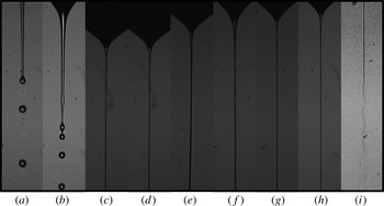
Images of the emitted jet at the minimum flow rate: (a) 1-decanol,
 $Q=0.4~\text{ml}~\text{h}^{-1}$
,
 $V=1740~\text{V}$
,
 $d_{j}=6.6~\unicode[STIX]{x03BC}\text{m}$
; (b) 1-octanol,
 $Q=0.5~\text{ml}~\text{h}^{-1}$
,
 $V=1600~\text{V}$
,
 $d_{j}=7.5~\unicode[STIX]{x03BC}\text{m}$
; (c) 3-
 $\text{ETG}+\text{LiCl}$
0.00005M,
 $Q=0.09~\text{ml}~\text{h}^{-1}$
,
 $V=2158~\text{V}$
,
 $d_{j}=1.7~\unicode[STIX]{x03BC}\text{m}$
; (d) 3-
 $\text{ETG}+\text{LiCl}$
0.0001M,
 $Q=0.09~\text{ml}~\text{h}^{-1}$
,
 $V=2231~\text{V}$
,
 $d_{j}=2.0~\unicode[STIX]{x03BC}\text{m}$
; (e) 3-
 $\text{ETG}+\text{LiCl}$
0.0005M,
 $Q=0.1~\text{ml}~\text{h}^{-1}$
,
 $V=2277~\text{V}$
,
 $d_{j}=1.7~\unicode[STIX]{x03BC}\text{m}$
; (f) 3-
 $\text{ETG}+\text{LiCl}$
0.001M,
 $Q=0.2~\text{ml}~\text{h}^{-1}$
,
 $V=2400~\text{V}$
,
 $d_{j}=2.5~\unicode[STIX]{x03BC}\text{m}$
; (g) 3-
 $\text{ETG}+\text{LiCl}$
0.002M,
 $Q=0.1~\text{ml}~\text{h}^{-1}$
,
 $V=2400~\text{V}$
,
 $d_{j}=1.7~\unicode[STIX]{x03BC}\text{m}$
; (h) 3-
 $\text{ETG}+\text{LiCl}$
0.005M,
 $Q=0.08~\text{ml}~\text{h}^{-1}$
,
 $V=2441~\text{V}$
,
 $d_{j}=1.3~\unicode[STIX]{x03BC}\text{m}$
; (i) 3-
 $\text{ETG}+\text{LiCl}$
0.007M,
 $Q=0.06~\text{ml}~\text{h}^{-1}$
,
 $V=2283~\text{V}$
,
 $d_{j}=1.7~\unicode[STIX]{x03BC}\text{m}$
. In all the cases, the inner diameter of the feeding capillary was 210
 $\unicode[STIX]{x03BC}\text{m}$
. The images show only a small portion of the liquid meniscus.

In the experiments, the liquid flow rate was reduced in steps of
 $0.1~\text{ml}~\text{h}^{-1}$
. For each flow rate, the electric potential was adjusted so that the apparent semiangle of the conical meniscus was approximately
 $49^{\circ }$
. This process was repeated until the steady cone-jet mode could not be established. The flow rate of the last steady cone-jet mode was taken as the minimum flow rate. Figure 4 shows images of the emitted jet at the minimum flow rate for all the working liquids. As will be shown in § 5.2, whipping was observed in all the experiments with
 $\text{ETG}+\text{LiCl}$
0.007M. In the rest of the cases, that jet instability did not occur.
5 Results
5.1 Numerical results
In the first part of this section, we present the simulation results obtained for two representative configurations among those examined experimentally in this work: 3-
 $\text{ETG}+\text{LiCl}$
0.0005M with
 $R_{i}=105~\unicode[STIX]{x03BC}\text{m}$
and 1-octanol with
 $R_{i}=550~\unicode[STIX]{x03BC}\text{m}$
. Then, we study the superficial charge relaxation in all the electrospraying realizations considered in this work. This section closes with some results for the viscosity- and polarity-dominated configurations. In all the cases, we will present results for flow rates very close to its corresponding minimum value. As will be shown in § 5.2, the applied voltages were selected for the minimum flow rates predicted from the linear stability analysis to coincide with those determined experimentally (when available).
Figure 5 shows the base flows calculated for
 $\unicode[STIX]{x1D6FD}=23.7$
,
 $\unicode[STIX]{x1D6FF}_{\unicode[STIX]{x1D707}}=0.174$
and
 $Q_{r}=7.74$
(3-
 $\text{ETG}+\text{LiCl}$
0.0005M), and
 $\unicode[STIX]{x1D6FD}=10$
,
 $\unicode[STIX]{x1D6FF}_{\unicode[STIX]{x1D707}}=2.29$
and
 $Q_{r}=2.98$
(1-octanol). In the former case, the viscous stresses arrange the flow towards the meniscus tip, which prevents the formation of recirculation cells. These cells arise in the latter case due to the accumulation of momentum at the cone apex, which increases the stagnation pressure there, and pushes back the liquid along the meniscus symmetry axis. This is a common behaviour in tip streaming (Tseng & Prosperetti Reference Tseng and Prosperetti2015) close to the minimum flow rate stability limit (Vega et al.
Reference Vega, Montanero, Herrada and Gañán-Calvo2010). The ratios between the jet and capillary diameters are 0.00434 and 0.0117 for 3-
 $\text{ETG}+\text{LiCl}$
0.0005M and 1-octanol, respectively and, therefore, the local character of the jet emission can be assumed. As will be shown in § 5.2, these values are consistent with those predicted by the scaling law (2.2). The equipotential lines show that the drop of voltage across the Taylor meniscus is negligible as compared to that taking place in the cone-jet transition region. A significant tangential electric field survives downstream far away from the meniscus. The fact that the equipotential lines become almost parallel to the jet’s free surface indicates that
 $E_{n}^{o}\gg E_{t}$
on that surface.
Base flows for (a)
 $\unicode[STIX]{x1D6FD}=23.7$
,
 $\unicode[STIX]{x1D6FF}_{\unicode[STIX]{x1D707}}=0.174$
and
 $Q_{r}=7.74$
, and (b)
 $\unicode[STIX]{x1D6FD}=10$
,
 $\unicode[STIX]{x1D6FF}_{\unicode[STIX]{x1D707}}=2.29$
and
 $Q_{r}=2.98$
. The lines in the inner and outer domains correspond to the streamlines and equipotential lines, respectively.

It is sometimes implicitly assumed that a base flow is stable if the numerical algorithm used to calculate it converges to a physically meaningful solution. In fact, this occurs with our method and capillary systems like liquid bridges (Vega et al.
Reference Vega, Montanero, Herrada and Ferrera2014), and seems quite reasonable in general if the algorithm is a time marching method. However, this assumption is not valid for our numerical procedure and the electrospray realizations analysed in this work. Figure 6 shows the eight eigenvalues with the larger growth factors
 $\unicode[STIX]{x1D714}_{i}$
characterizing the linear stability of the two base flows described above (open symbols). As can be observed, the spectrum of eigenvalues remains in the stable half-plane. On the contrary, the dominant eigenvalue crosses the boundary
 $\unicode[STIX]{x1D714}_{i}=0$
for
 $Q_{r}=6.0$
and 2.32 in the 3-
 $\text{ETG}+\text{LiCl}$
0.0005M and 1-octanol case, respectively. This loss of stability has an oscillatory character because the real part
 $\unicode[STIX]{x1D714}_{r}$
of the dominant eigenvalue is different from zero. In the two cases considered,
 $\unicode[STIX]{x1D714}_{r}\sim 1$
, which indicates that the period of the oscillation responsible for instability scales with the meniscus capillary time
 $t_{c}$
. This result suggests that the unstable mode perturbs not only the region where is originated but also the whole liquid meniscus shape. It must be noted that one cannot anticipate the stability/instability from the simple inspection of the base flows because they exhibit essentially the same features independently of their stability character. In fact, we do not observe any bifurcation when the numerical solution crosses the stability limit.
(a) Eigenvalues for
 $\unicode[STIX]{x1D6FD}=23.7$
,
 $\unicode[STIX]{x1D6FF}_{\unicode[STIX]{x1D707}}=0.147$
and
 $Q_{r}=7.74$
(open symbols) and 6.0 (solid symbols). (b) Eigenvalues for
 $\unicode[STIX]{x1D6FD}=10$
,
 $\unicode[STIX]{x1D6FF}_{\unicode[STIX]{x1D707}}=2.29$
and
 $Q_{r}=2.98$
(open symbols) and 2.32 (solid symbols).

The dependence of the eigenvalue responsible for instability with respect to the ejected flow rate is shown in figure 7. The minimum flow rate corresponds to the intersection between the curve
 $\unicode[STIX]{x1D714}_{i}(Q_{r})$
and the axis
 $\unicode[STIX]{x1D714}_{i}=0$
. As can be observed, the oscillation frequency depends slightly on the injected flow rate, and is considerably smaller for 3-
 $\text{ETG}+\text{LiCl}$
0.0005M.
Real (a) and imaginary (b) part of the eigenvalue responsible for instability as a function of
 $Q_{r}$
. The results were calculated for
 $\unicode[STIX]{x1D6FD}=23.7$
and
 $\unicode[STIX]{x1D6FF}_{\unicode[STIX]{x1D707}}=0.147$
(solid symbols), and for
 $\unicode[STIX]{x1D6FD}=10$
and
 $\unicode[STIX]{x1D6FF}_{\unicode[STIX]{x1D707}}=2.29$
(open symbols).

As will be seen below, the driving electric shear stress survives and accelerates the jet downstream over a long distance from the electrified meniscus. To make sure that the outflow boundary conditions do not produce significant errors, the numerical simulation must consider a very long computational domain. For this reason, the loss of stability of the base flow can be caused by either the destabilization of the liquid source or the convective instability associated with the growth of capillary waves far away from that source. The former case does correspond to the breakdown of the steady cone-jet mode, while the latter is associated with the classical Rayleigh instability in a steadily emitted jet (Rayleigh Reference Rayleigh1878).
In order to distinguish the two phenomena mentioned above, the eigenmode responsible for instability at the minimum flow rate must be analysed. Figure 8 shows the magnitude
 $|\unicode[STIX]{x1D6FF}e_{k}|=|u_{o}\unicode[STIX]{x1D6FF}u+w_{0}\unicode[STIX]{x1D6FF}w|$
of the perturbation kinetic energy per unit mass,
 $\unicode[STIX]{x1D6FF}e_{k}=(u_{0}\unicode[STIX]{x1D6FF}u+w_{0}\unicode[STIX]{x1D6FF}w)\text{e}^{-\text{i}\unicode[STIX]{x1D714}t}$
, along the free surface and relative to its value
 $e_{k}=1/2~(u_{0}^{2}+w_{0}^{2})$
in the base flow. In these expressions,
 $u_{0}$
(
 $w_{0}$
) and
 $\unicode[STIX]{x1D6FF}u$
(
 $\unicode[STIX]{x1D6FF}w$
) represent the base flow value and perturbation amplitude of the radial (axial) component of the velocity field, respectively. The kinematic compatibility condition (3.5) links the oscillation amplitude of the two components of the velocity field at the free surface to the oscillation of that surface. In fact, the slenderness approximation of that condition reduces to
 $\hat{F}=\unicode[STIX]{x1D6FF}u/(\text{i}\unicode[STIX]{x1D714})$
, where
 $\hat{F}$
stands for the perturbation amplitude of the free surface position. This equation suggests that
 $|\unicode[STIX]{x1D6FF}e_{k}|/e_{k}$
may constitute a good indicator of where the free surface deformation becomes greater at the initial phase of the instability growth. Other variables could be used for that purpose too.
(a,b) Perturbation amplitude of the kinetic energy
 $|\unicode[STIX]{x1D6FF}e_{k}|$
along the free surface relative to its value
 $e_{k}$
in the base flow. The perturbations are normalized so that the maximum value of
 $|\unicode[STIX]{x1D6FF}e_{k}|/e_{k}$
is equal to one. (c,d) Free surface position
 $F$
, bulk current intensity
 $I_{b}$
and surface current intensity
 $I_{s}$
as a function of the axial position
 $z$
. The results were calculated for
 $\unicode[STIX]{x1D6FD}=23.7$
,
 $\unicode[STIX]{x1D6FF}_{\unicode[STIX]{x1D707}}=0.147$
and
 $Q_{r}=7.74$
(a,c), and
 $\unicode[STIX]{x1D6FD}=10$
,
 $\unicode[STIX]{x1D6FF}_{\unicode[STIX]{x1D707}}=2.29$
and
 $Q_{r}=2.98$
(b,d).

In the two cases analysed in figure 8,
 $|\unicode[STIX]{x1D6FF}e_{k}|/e_{k}$
reaches its maximum value in the cone-jet transition region, close to the jet section where the conduction intensity equals the surface convection of charges. This result indicates that the electrified meniscus does become unstable for flow rates smaller than the threshold, and may suggest the critical role played by the singular fluidic structure arising in the cone-jet transition region. The relative amplitude
 $|\unicode[STIX]{x1D6FF}e_{k}|/e_{k}$
also takes large values in the liquid meniscus contour, which confirms that the perturbation causes the oscillation of the entire meniscus.
The values of
 $E_{t}$
and
 $E_{n}^{o}$
in the two cases analysed in figure 9 are consistent with the scaling laws. Specifically,
 $E_{t}/(E_{n}^{o}Q_{r}^{-1/2})\sim 1$
(2.4) and
 $E_{n}^{o}/E_{o}\sim 1$
(2.6) at the section
 $I_{b}=I_{s}$
in the two simulations. This consistency was also obtained for the other three cases not dominated by either viscosity or polarity. In this work, we define the cone-jet transition region as that corresponding to the interval
 $-0.5\leqslant \log _{10}(I_{s}/I_{b})\leqslant 0.5$
(i.e.
 $I_{s}$
and
 $I_{b}$
are of the same order of magnitude). According to the results shown in 9,
 $L/(d_{0}Q_{r})\sim 1$
(2.7) in both cases.
As mentioned in § 2.3, there is a general consensus about the absence of net free charge in the cone-jet bulk. In fact, this constitutes the essential approximation of the leaky dielectric model solved in this work and by other researchers (Yan et al.
Reference Yan, Farouk and Ko2003; Higuera Reference Higuera2003, Reference Higuera2010). Fernández de la Mora (Reference Fernández de la Mora2007) defined the lack of charge relaxation as the inability of the electric conduction from the bulk into the free surface to establish the electrostatic charge density
 $\unicode[STIX]{x1D70E}_{e}=\unicode[STIX]{x1D700}_{o}E_{n}^{o}$
in the meniscus tip; in other words, to screen the electric field normal to the free surface so that
 $\unicode[STIX]{x1D6FD}E_{n}^{i}\ll E_{n}^{o}$
in that region. Figure 9 shows that the values of
 $\unicode[STIX]{x1D6FD}E_{n}^{i}$
are considerably smaller than, but non-negligible as compared to,
 $E_{n}^{o}$
in the cone-jet transition region for both 1-octanol and 3-
 $\text{ETG}+\text{LiCl}$
0.0005M. The maximum value
 $(\unicode[STIX]{x1D6FD}E_{n}^{i}/E_{n}^{o})_{max}$
over the free surface of the ratio
 $\unicode[STIX]{x1D6FD}E_{n}^{i}/E_{n}^{o}$
is reached very close to the section
 $I_{s}=I_{b}$
.
(a,b) Free surface position
 $F$
, bulk current intensity
 $I_{b}$
and surface current intensity
 $I_{s}$
as a function of the axial position
 $z$
. (c,d) Tangential and normal components of the inner and outer electric fields at the free surface. The results were calculated for
 $\unicode[STIX]{x1D6FD}=23.7$
,
 $\unicode[STIX]{x1D6FF}_{\unicode[STIX]{x1D707}}=0.147$
and
 $Q_{r}=7.74$
(a,c), and for
 $\unicode[STIX]{x1D6FD}=10$
,
 $\unicode[STIX]{x1D6FF}_{\unicode[STIX]{x1D707}}=2.29$
and
 $Q_{r}=2.98$
(b,d). The symbols correspond to the results obtained when the number of collocation points in the radial direction was doubled.

As explained in § 2.3, one may expect
 $\unicode[STIX]{x1D6FD}E_{n}^{i}$
to be commensurate with
 $E_{n}^{o}$
when the charge relaxation time
 $t_{e}$
is commensurate with the residence time
 $t_{r}$
of a free surface element in the cone-jet transition region. In order to verify this expectation quantitatively, we calculate the residence time
 $t_{r}$
of the free surface element in that interval as
 $$\begin{eqnarray}t_{r}=\int _{s_{i}}^{s_{f}}\frac{\text{d}s}{v_{s}},\end{eqnarray}$$
where
 $s_{i}$
and
 $s_{f}$
are the intrinsic coordinates of the inlet and outlet sections of the cone-jet transition region. The values of the ratio
 $t_{e}/t_{r}$
for 3-
 $\text{ETG}+\text{LiCl}$
0.0005M and 1-octanol are 0.32 and 0.098, respectively. Interestingly,
 $(\unicode[STIX]{x1D6FD}E_{n}^{i}/E_{n}^{o})_{max}=0.322$
for 3-
 $\text{ETG}+\text{LiCl}$
0.0005M and, therefore,
 $\unicode[STIX]{x1D6FD}E_{n}^{i}$
cannot be neglected as compared with
 $E_{n}^{o}$
even though the electric relaxation time is one order of magnitude smaller than the residence one. Therefore, one can safely assume that
 $\unicode[STIX]{x1D6FD}E_{n}^{i}$
is negligible in the cone-jet transition region only if there is true disparity (two or more orders of magnitude) between the two characteristic times.
Figure 10 shows the ratios
 $t_{e}/t_{r}$
and
 $(\unicode[STIX]{x1D6FD}E_{n}^{i}/E_{n}^{o})_{max}$
for all the simulations at the minimum flow rate stability limit. As can be observed,
 $t_{e}$
is considerably smaller than
 $t_{r}$
in all the realizations except for the high-polarity case, where
 $t_{e}\simeq t_{r}$
(Gañán-Calvo et al.
Reference Gañán-Calvo, Rebollo-Muñoz and Montanero2013). However,
 $\unicode[STIX]{x1D6FD}E_{n}^{i}$
is truly negligible as compared to
 $E_{n}^{o}$
only in the high-viscosity case, for which
 $t_{e}\ll t_{r}$
. It must be noted that the existence of significant inner electric fields in our simulations do not invalidate the scaling laws
 $\unicode[STIX]{x1D70E}\sim \unicode[STIX]{x1D700}_{o}E_{n}^{o}$
and
 $\text{I}\sim (E_{n}^{o})^{2}$
(I is the electrostatic term introduced in (5.2)), because
 $E_{n}^{o}\sim E_{n}^{o}-\unicode[STIX]{x1D6FD}E_{n}^{i}$
and
 $(E_{n}^{o})^{2}\sim (E_{n}^{o})^{2}-\unicode[STIX]{x1D6FD}(E_{n}^{i})^{2}$
in all the cases analysed. We have verified that the disparity between the electric and hydrodynamic characteristic times increases with the flow rate. For instance,
 $t_{e}/t_{r}=0.12$
for 3-
 $\text{ETG}+\text{LiCl}$
0.0005M and
 $Q_{r}=77.4$
.
Ratios
 $t_{e}/t_{r}$
(open symbols) and
 $(\unicode[STIX]{x1D6FD}E_{n}^{i}/E_{n}^{o})_{max}$
(solid symbols) at the minimum flow rate stability limit. The values of
 $\unicode[STIX]{x1D6FD}$
,
 $\unicode[STIX]{x1D6FF}_{\unicode[STIX]{x1D707}}$
and
 $Q_{r}$
are shown in table 2 (for 1-octanol, we chose the case with largest value of
 $\unicode[STIX]{x1D6EC}$
).

One may conclude that
 $t_{e}\sim t_{r}$
does not hold in general for the cone-jet transition region. Fernandez de la Mora & Loscertales (Reference Fernandez de la Mora and Loscertales1994) assumed that
 $t_{e}\sim t_{r}$
in a cone tip zone with size of the order of
 $d_{j}$
. Our result does not necessarily contradict that assumption because the size of that zone and that of the cone-jet transition region defined here are not generally commensurate with each other (2.7). In fact, caution must be taken when discussing the relative magnitude of the electric relaxation time and the residence time because the latter significantly depends on the definition of the cone-jet transition region.
In the one-dimensional (slenderness) approximation, the momentum equation in the
 $z$
-direction becomes (Gañán-Calvo Reference Gañán-Calvo1999):
 $$\begin{eqnarray}\underbrace{\frac{\unicode[STIX]{x1D712}}{2}\left[(E_{n}^{o})^{2}-\unicode[STIX]{x1D6FD}(E_{n}^{i})^{2}\right]_{z}}_{\text{I}}+\underbrace{\unicode[STIX]{x1D712}\frac{\unicode[STIX]{x1D6FD}-1}{2}\left[(E^{t})^{2}\right]_{z}}_{\text{II}}+\underbrace{\frac{2\unicode[STIX]{x1D70E}E_{t}}{F}}_{\text{III}}=\underbrace{\left(\frac{1}{F}\right)_{z}}_{\text{IV}}+\underbrace{\left(\frac{{\mathcal{Q}}^{2}}{2F^{4}}\right)_{z}}_{\text{V}}+\underbrace{\frac{6Oh{\mathcal{Q}}}{F^{2}}\left(\frac{F_{z}}{F}\right)_{z}}_{\text{VI}}.\end{eqnarray}$$
The terms of (5.2) have been grouped into driving (left-hand side) and resistant (right-hand side) forces. The first, second, and last addends on the left-hand side of (5.2) are generally referred to as the electrostatic, polarization and electric tangential forces per unit volume, respectively (Gañán-Calvo Reference Gañán-Calvo1999). The terms on the right-hand side of (5.2) correspond to surface tension, inertia and viscosity, respectively. Figure 11 shows the values taken by the six terms of (5.2) for 3-
 $\text{ETG}+\text{LiCl}$
0.0005M and 1-octanol. The area enclosed by the curves equals the work done/energy consumed per unit volume by the corresponding term.
(a–f) Terms I–VI of the slenderness model (5.2) as a function of the axial position
 $z$
. (g,h) Free surface position
 $F$
, bulk current intensity
 $I_{b}$
and surface current intensity
 $I_{s}$
as a function of the axial position
 $z$
. The results were calculated for
 $\unicode[STIX]{x1D6FD}=23.7$
,
 $\unicode[STIX]{x1D6FF}_{\unicode[STIX]{x1D707}}=0.147$
and
 $Q_{r}=7.74$
(a,c,e,g), and for
 $\unicode[STIX]{x1D6FD}=10$
,
 $\unicode[STIX]{x1D6FF}_{\unicode[STIX]{x1D707}}=2.29$
and
 $Q_{r}=2.98$
(b,d,f,h).
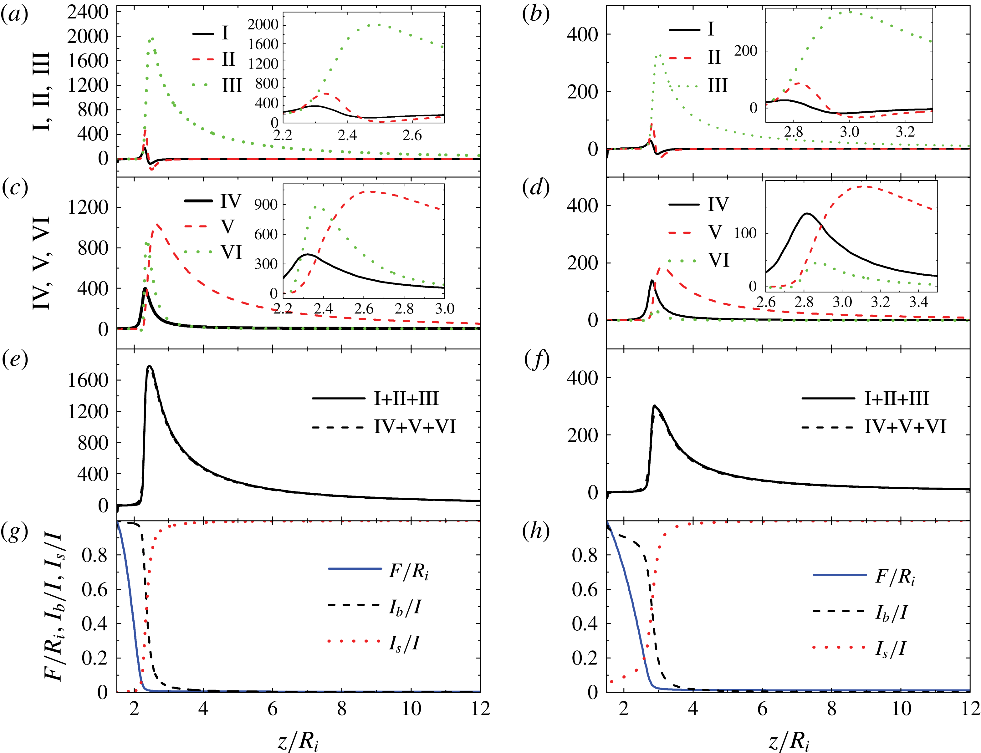
The electric tangential force is the major source of energy both in the cone-jet transition region and throughout the jet. The dominant role played by this force was already pointed out by Higuera (Reference Higuera2010) using numerical simulations in the Stokes limit. Both the electrostatic and polarization forces are subdominant. The fact that the electrostatic suction transfers much less energy than the tangential force differs from the scaling analysis prediction for large flow rates (§ 2.1), which concludes that these effects commensurate with each other. Most of the work done by the electric forces is converted into kinetic energy. The viscous force arises against the liquid ejection for
 $\unicode[STIX]{x1D6FF}_{\unicode[STIX]{x1D707}}=0.147$
, while surface tension becomes the largest resistant force for
 $\unicode[STIX]{x1D6FF}_{\unicode[STIX]{x1D707}}=2.29$
. The electrostatic and polarization forces push the liquid in the cone-jet transition region, while stand against the liquid ejection behind that region. Graph (c) shows the accuracy of the one-dimensional approximation throughout the whole liquid domain even for the least viscous case, which exhibits recirculation in the electrified meniscus (figure 5).
In order to elucidate the role played by the electrostatic and tangential forces, we run simulations ‘switching off’ the terms
 $\unicode[STIX]{x1D712}/2[(E_{n}^{o})^{2}-\unicode[STIX]{x1D6FD}(E_{n}^{i})^{2}]$
and
 $\unicode[STIX]{x1D712}\unicode[STIX]{x1D70E}E_{t}$
in (3.6) and (3.7), respectively. When the electrostatic suction is switched off, the numerical method does not converge to a steady solution. This result indicates the importance of this force in stretching the meniscus and forming the ‘liquid nozzle’ through which the jet is emitted. It also shows that the cone-jet mode stability cannot be analysed just in terms of the balance between the dominant driving and resistant forces because subdominant stresses are also necessary to produce steady jetting. If the electric shear stress
 $\unicode[STIX]{x1D712}\unicode[STIX]{x1D70E}E_{t}$
is turned off, the numerical algorithm for 1-octanol does not converge either, while the 3-
 $\text{ETG}+\text{LiCl}$
0.0005M jet losses most of its kinetic energy and the cone-jet mode becomes linearly unstable (figure 12).
Free surface position
 $F(z)$
(a) and eigenvalues (b) for
 $\unicode[STIX]{x1D6FD}=23.7$
,
 $\unicode[STIX]{x1D6FF}_{\unicode[STIX]{x1D707}}=0.147$
and
 $Q_{r}=7.74$
. In (a) the solid and dashed lines correspond to the exact solution and that calculated when the electric shear stress is not considered, respectively. In (b) the open and solid symbols correspond to the exact solution and that calculated when the electric shear stress is not taken into account, respectively.

We analyse the forces arising for large values of
 $\unicode[STIX]{x1D6FF}_{\unicode[STIX]{x1D707}}$
and
 $\unicode[STIX]{x1D6FD}$
in figure 13. The electric tangential force III is dominant in the cone-jet transition region of the two cases, although the polarization force exhibits a sharp peak in front of that region in the high-polarity case. The polarization force stretches the transition region and moves the zone dominated by charge convection away from the meniscus. In fact, the section where
 $I_{b}=I_{s}$
is shifted beyond the cone apex in the high-polarity case. As claimed by Gañán-Calvo et al. (Reference Gañán-Calvo, Rebollo-Muñoz and Montanero2013), the viscous force VI becomes of the order of inertia in the cone-jet transition region for small
 $\unicode[STIX]{x1D6FF}_{\unicode[STIX]{x1D707}}$
. The increase of this resistant force as the flow rate decreases may explain the cone-jet mode instability originated in that region. As mentioned above, the polarization force becomes the dominant driving force in front of the jet emission region for large
 $\unicode[STIX]{x1D6FD}$
. The liquid acceleration caused by this force shortens the liquid meniscus, sharply reducing the free surface radius in front of the apex, which increases the capillary stress there. However, the polarization force opposes to the ejection (II becomes negative) and is of the order of inertia in the cone-jet transition region (Gañán-Calvo et al.
Reference Gañán-Calvo, Rebollo-Muñoz and Montanero2013). As shown in figure 10, the integral (5.1) gives
 $t_{e}/t_{r}=0.643$
and 1.06 for the viscous and polarization case, respectively. The fact that
 $t_{e}$
becomes of the order of
 $t_{r}$
for very polar liquids close to the minimum flow rate stability limit can be anticipated from the scaling laws in § 2.2 (Gañán-Calvo et al.
Reference Gañán-Calvo, Rebollo-Muñoz and Montanero2013).
(a–f) Terms I–VI of the slenderness model (5.2) as a function of the axial position
 $z$
. (g,h) Free surface position
 $F$
, bulk current intensity
 $I_{b}$
and surface current intensity
 $I_{s}$
as a function of the axial position
 $z$
. The results were calculated for
 $\unicode[STIX]{x1D6FD}=23.7$
,
 $\unicode[STIX]{x1D6FF}_{\unicode[STIX]{x1D707}}=0.0108$
and
 $Q_{r}=66.2$
(a,c,e,g), and for
 $\unicode[STIX]{x1D6FD}=70$
,
 $\unicode[STIX]{x1D6FF}_{\unicode[STIX]{x1D707}}=2.29$
and
 $Q_{r}=7.49$
(b,d,f,h).

5.2 Experimental results
For sufficiently small values of the ratios
 $d_{j}/R_{i}$
and
 $L/R_{i}$
, the flow in the critical cone-jet transition region is not essentially affected by the boundary conditions and, therefore, one expects that
 $Q_{r\,min}=Q_{r\,min}(\unicode[STIX]{x1D6FD},\unicode[STIX]{x1D6FF}_{\unicode[STIX]{x1D707}})$
. As explained in § 2.1, experimental values of
 $Q_{r\,min}$
obtained by different authors have been explained in terms of the scaling law
 $Q_{r\,min}\sim \unicode[STIX]{x1D6FD}^{\unicode[STIX]{x1D703}_{1}}\unicode[STIX]{x1D6FF}_{\unicode[STIX]{x1D707}}^{\unicode[STIX]{x1D703}_{2}}$
for
 $\unicode[STIX]{x1D6FD}\unicode[STIX]{x1D6FF}_{\unicode[STIX]{x1D707}}\ll 1$
and
 $\unicode[STIX]{x1D6FD}\unicode[STIX]{x1D6FF}_{\unicode[STIX]{x1D707}}\gg 1$
, assuming self-similarity (Barenblatt Reference Barenblatt2003) in those two limiting regimes (Gañán-Calvo et al.
Reference Gañán-Calvo, Rebollo-Muñoz and Montanero2013). Because the experimental values for the intermediate range
 $\unicode[STIX]{x1D6FD}\unicode[STIX]{x1D6FF}_{\unicode[STIX]{x1D707}}\sim 1$
are scarce, we measured the minimum flow rate in that range. Also, we examined the break-up of the emitted jet at the minimum flow rate stability limit with a very high spatio-temporal resolution. The results are presented and compared with numerical simulations in this section.
We define the jet’s level of electrification (the Taylor number) as the ratio of the electric stress normal to the jet’s free surface,
 $\unicode[STIX]{x1D700}_{o}(E_{n}^{o})^{2}$
, to the capillary pressure
 $\unicode[STIX]{x1D6FE}/(d_{j}/2)$
, i.e.
 $$\begin{eqnarray}\unicode[STIX]{x1D6E4}=\frac{\unicode[STIX]{x1D700}_{o}(E_{n}^{o})^{2}}{\unicode[STIX]{x1D6FE}/(d_{j}/2)}.\end{eqnarray}$$
Sufficiently far away from the meniscus, the superficial charge relaxes to its electrostatic value (
 $\unicode[STIX]{x1D6FD}E_{n}^{i}\ll E_{n}^{o}$
) and conduction vanishes (
 $I\simeq I_{s}$
) (figure 9). In that region,
 $E_{n}^{o}\simeq \unicode[STIX]{x1D70E}/\unicode[STIX]{x1D700}_{o}$
,
 $\unicode[STIX]{x1D70E}=Id_{j}/(4Q)$
and, therefore, the level of electrification (5.3) can be calculated as
 $$\begin{eqnarray}\unicode[STIX]{x1D6E4}=\frac{I^{2}d_{j}^{3}}{32Q^{2}\unicode[STIX]{x1D6FE}\unicode[STIX]{x1D700}_{o}}.\end{eqnarray}$$
The jet emitted by a Taylor cone in a hydrodynamically passive dielectric medium may develop the so-called whipping instability for sufficiently large values of the Taylor number (figure 4
i) (Hohman et al.
Reference Hohman, Shin, Rutledge and Brenner2001; Eggers & Villermaux Reference Eggers and Villermaux2008; Yang et al.
Reference Yang, Duan, Li and Deng2014). This instability gives rise to non-axisymmetric (lateral) oscillations which cause the fast and violent lashes of the charged jet. Rayleigh (Reference Rayleigh1881) originally explained this phenomenon in terms of the balance between the decrease of electric energy and increase of interfacial energy caused by the lateral displacement of a charged jet. His calculations for a perfectly conductor, apolar and inviscid cylinder in the absence of an externally applied electric field led to the so-called Rayleigh limit
 $\unicode[STIX]{x1D6E4}_{R}=3/2$
for the electrification level of that cylinder. The whipping instability in a perfectly conductor jet can also be explained as follows: if a small portion of the jet moves slightly off its axis, the charge re-distributes instantaneously along the jet surface accumulating in the ridges and valleys of the deformed interface, in such a way that the electrical forces will push that portion farther away from the axis (Hohman et al.
Reference Hohman, Shin, Rutledge and Brenner2001).
Figure 14(a) shows the jet’s electrification level (5.4) in all the cone-jet mode experimental realizations. Whipping was observed for
 $\unicode[STIX]{x1D6E4}\gtrsim 3$
(in this case, the jet diameter was measured in front of the whipping instability region). This value clearly exceeds the Rayleigh limit, which can be explained in terms of the complex interplay among charge relaxation, viscosity, polarization force and the external axial field taking place in our problem (Mestel Reference Mestel1996). In the stable jets with levels of electrification exceeding the Rayleigh limit, the jet’s capillary time
 $t_{cj}=(\unicode[STIX]{x1D70C}d_{j}^{3}/\unicode[STIX]{x1D6FE})^{1/2}$
took similar values to those of the electric relaxation time
 $t_{e}$
, while the jet’s Ohnesorge number
 $Oh_{j}=\unicode[STIX]{x1D707}(\unicode[STIX]{x1D70C}d_{j}\unicode[STIX]{x1D6FE})^{-1/2}$
increased up to values of the order of 10. For instance,
 $t_{cj}\simeq 0.217~\unicode[STIX]{x03BC}\text{s}$
,
 $t_{e}\simeq 0.223~\unicode[STIX]{x03BC}\text{s}$
and
 $Oh_{j}\simeq 5.16$
for the case of figure 4(h). According to the scaling laws (2.2) and (2.5),
 $\unicode[STIX]{x1D6E4}$
should scale as
 $Q_{r}^{1/2}$
(with a small prefactor). The deviation of the experimental data from that prediction can be explained in terms of the lack of accuracy of those scaling laws for
 $Q_{r}\lesssim 1$
, which is magnified by the exponents of
 $I$
and
 $d_{j}$
in (5.4).
The convective instability of the electrified jet emitted in electrospraying is a prerequisite to achieving the steady cone-jet mode (Huerre & Monkewitz Reference Huerre and Monkewitz1990). Figure 14(b) shows the values of the jet’s capillary and Reynolds numbers,
 $$\begin{eqnarray}Ca_{j}=\frac{v_{j}\unicode[STIX]{x1D707}}{\unicode[STIX]{x1D6FE}}\quad \text{and}\quad Re_{j}=\frac{\unicode[STIX]{x1D70C}v_{j}d_{j}}{2\unicode[STIX]{x1D707}},\end{eqnarray}$$
in all the cone-jet mode experimental realizations. The line shows the convective-to-absolute instability transition calculated for a non-electrified jet (Leib & Goldstein Reference Leib and Goldstein1986). Although this transition is affected by the electrification level, axial electric field intensity and permittivity, the classical Leib and Goldstein prediction is expected to constitute a good approximation for a significant part of the parameter space (López-Herrera, Gañán-Calvo & Herrada Reference López-Herrera, Gañán-Calvo and Herrada2010). In fact, all the jets produced in our experiments were convectively unstable according to that approximation. The cloud of points corresponding to previous works, and collected by López-Herrera et al. (Reference López-Herrera, Gañán-Calvo and Herrada2010), are generally located farther away from the Leib and Goldstein curve than those of the present work. In some cases, this could be due to the fact that the authors did not intend to reach the minimum flow rate in their experiments. In other cases, the instability arose in the cone-jet transition region long before the jet became absolutely unstable. Very few of those points cross the instability transition curve for an non-electrified jet, probably because of the stabilizing electric effects occurring in those cases.
(a) Jet electrification level
 $\unicode[STIX]{x1D6E4}$
as a function of the dimensionless flow rate
 $Q_{r}$
in all the cone-jet mode realizations. The open and solid symbols correspond to steady jetting and whipping, respectively. The solid line indicates the slope of the power law
 $\unicode[STIX]{x1D6E4}\propto Q_{r}^{1/2}$
. (b) Jet capillary number
 $Ca_{j}$
and Reynolds number
 $Re_{j}$
in all the cone-jet mode realizations. The open and solid symbols correspond to steady jetting and whipping, respectively (the labels are those in the left-hand graph). The grey symbols correspond to previous experimental results gathered by López-Herrera et al. (Reference López-Herrera, Gañán-Calvo and Herrada2010). The line corresponds to the convective–absolute instability transition for a non-electrified jet (Leib & Goldstein Reference Leib and Goldstein1986).

The jet’s diameter
 $d_{j}$
and electric intensity
 $I$
in all the experimental cone-jet mode realizations are plotted as a function of the dimensionless flow rate
 $Q_{r}$
in figure 15. The scaling laws (2.2) and (2.5) reasonably fit the experimental data, although the prefactor of
 $d_{j}/d_{o}(Q_{r})$
for small
 $Q_{r}$
seems to be slightly different from that for large
 $Q_{r}$
. The diameters in the experiments where whipping took place significantly deviated from the scaling law, probably because they were measured before the jet stretching ended. The diameters and electric currents calculated from the simulation also approximately match the scaling laws, even for small
 $\unicode[STIX]{x1D6FF}_{\unicode[STIX]{x1D707}}$
(large
 $Q_{r}$
). The only exception is the intensity of the high-polarity case, which deviates significantly from the trend of the rest of simulations. In fact, the current intensity for very polar liquids is expected to follow a different law from that for low and moderate polarity, as predicted by Gañán-Calvo (Reference Gañán-Calvo2004).
The jet’s diameter (a) and current intensity (b) as a function of the dimensionless flow rate
 $Q_{r}$
in all the cone-jet mode realizations. The open and solid symbols correspond to steady jetting and whipping, respectively. The big red circles are simulation results. The arrows indicate the results for large polarity (
 $\unicode[STIX]{x1D6FD}=70$
). The solid lines are the functions
 $d_{j}/d_{o}=0.85Q_{r}^{1/2}$
and
 $I/I_{o}=2.5Q_{r}^{1/2}$
(scaling laws (2.2) and (2.5), respectively).

Figure 16 shows the values of
 $Q_{r}/\unicode[STIX]{x1D6FD}$
and
 $\unicode[STIX]{x1D6FD}\unicode[STIX]{x1D6FF}_{\unicode[STIX]{x1D707}}$
of steady cone-jet mode realizations. The grey symbols represent the data gathered from different authors and plotted in figure 2 of Gañán-Calvo et al. (Reference Gañán-Calvo, Rebollo-Muñoz and Montanero2013). The open symbols correspond to experimental realizations conducted in the present work with a capillary
 $R_{i}=105~\unicode[STIX]{x03BC}\text{m}$
in radius. The new experiments with 3-ETG allows one to draw the instability curve between the polarization and viscous regimes obtained for
 $(\unicode[STIX]{x1D6FD}\unicode[STIX]{x1D6FF}_{\unicode[STIX]{x1D707}})^{-1}\ll 1$
and
 $(\unicode[STIX]{x1D6FD}\unicode[STIX]{x1D6FF}_{\unicode[STIX]{x1D707}})^{-1}\gg 1$
, respectively. The big white circles show the experiments conducted with 1-octanol and
 $R_{i}=550~\unicode[STIX]{x03BC}\text{m}$
. The comparison with the small circles shows the stabilization effect achieved when the diameter of the feeding capillary is reduced. It must be noted that the minimum flow rate is expected to be sensitive to the capillary diameter only if the ratio
 $2R_{i}/d_{j}$
is of the order of or smaller than, say,
 $10^{2}$
. This only occurs for small enough conductivities and feeding capillary diameters. In our work, this twofold condition was verified only for the three alcohols, and not for the 3-
 $\text{ETG}+\text{LiCl}$
solutions. Similarly, the jets produced by other authors and represented on the right side of figure 16 were sufficiently small in terms of the feeding capillary diameter, and the latter is not expected to affect the results. Only the results on the left side of the figure could be influenced by the capillary diameter, which might partially explain the small flow rates achieved in that part of the figure. The dashed and solid lines are the scaling laws
 $Q_{r\,min}=0.2\unicode[STIX]{x1D6FD}$
and
 $Q_{r\,min}=\unicode[STIX]{x1D6FF}_{\unicode[STIX]{x1D707}}^{-1}$
for the polar and viscous limits, respectively (Gañán-Calvo et al.
Reference Gañán-Calvo, Rebollo-Muñoz and Montanero2013). Both the new experimental results and the numerical ones are consistent with those laws. The stabilization effect due to the size of the feeding capillary explains why the prefactor of the scaling law
 $Q_{r\,min}\sim \unicode[STIX]{x1D6FD}$
derived by Gañán-Calvo et al. (Reference Gañán-Calvo, Rebollo-Muñoz and Montanero2013) was much smaller than unity.
Steady cone-jet mode realizations. The grey symbols are the data gathered from different authors (figure 2 in Gañán-Calvo et al. (Reference Gañán-Calvo, Rebollo-Muñoz and Montanero2013)). The white symbols correspond to the experimental results obtained in this work with a capillary
 $R_{i}=105~\unicode[STIX]{x03BC}\text{m}$
in radius. The big white circles show the experiments conducted with 1-octanol and
 $R_{i}=550~\unicode[STIX]{x03BC}\text{m}$
. The big red circles and big blue squares are marginally stable basic flows corresponding to
 $R_{i}=105~\unicode[STIX]{x03BC}\text{m}$
and
 $R_{i}=550~\unicode[STIX]{x03BC}\text{m}$
, respectively, for the voltages shown in table 2. The dashed and solid lines are the scaling laws
 $Q_{r\,min}=0.2\unicode[STIX]{x1D6FD}$
and
 $Q_{r\,min}=\unicode[STIX]{x1D6FF}_{\unicode[STIX]{x1D707}}^{-1}$
for the polar and viscous limits, respectively.

The feeding capillary stabilization effect is illustrated in more detail in figure 17, which shows that the minimum flow rate becomes independent of the capillary radius only for
 $\unicode[STIX]{x1D6EC}\gtrsim 80$
, which corresponds to diameters
 $2R_{i}\gtrsim 1~\text{mm}$
(two orders of magnitude larger than the jet diameter). This conclusion is valid for a constant capillary-to-counterelectrode distance (
 $H^{\prime }/d_{0}=71.4$
), and when that distance was proportional to the capillary diameter (
 $H^{\prime }/(2R_{i})=4.76$
). We also verified that the minimum flow rates were essentially the same when polarity was inverted.
Minimum flow rate
 $Q_{r\,min}=Q_{\,min}/Q_{o}$
as a function of the feeding capillary diameter
 $\unicode[STIX]{x1D6EC}=2R_{i}/d_{o}$
for
 $\unicode[STIX]{x1D6FD}=10$
and
 $\unicode[STIX]{x1D6FF}_{\unicode[STIX]{x1D707}}=2.29$
(1-octanol). The solid and open symbols correspond to
 $H^{\prime }/(2R_{i})=4.76$
and
 $H^{\prime }/d_{0}=71.4$
, respectively. The red big circles are the corresponding marginally stable basic flows for the voltages shown in table 2.

The electric boundary conditions prescribed in the simulations (the analytical solution for the far-field electric potential) do not coincide with those imposed experimentally (an electric potential applied to the end of the feeding capillary in front of a ground electrode). For this reason, we adjusted the applied voltage in the simulations for the numerical and experimental values of the minimum flow rate to coincide with each other. The resulting numerical voltages deviated from the experimental ones between approximately 8 % and 25 %, depending on the case (see table 2). Based on these results, one can conclude that there is good agreement between the stability limits predicted from the asymptotic linear stability analysis and the corresponding experimental values. This indicates that the loss of stability is caused by the long-term growth of the dominant global mode, as implicitly assumed in that analysis (Theofilis Reference Theofilis2011). In this sense, electrospray behaves differently from other steady jetting configurations like gaseous flow focusing, where instability can also be caused by the short-term superposition of the linear perturbations (Cruz-Mazo et al. Reference Cruz-Mazo, Herrada, Gañán-Calvo and Montanero2017).
Jet diameter, current intensity and minimum flow rate measured experimentally and calculated numerically. The superscripts ‘exp’ and ‘num’ stand for the values obtained experimentally and numerically, respectively. The voltages in the numerical simulations were selected so that the numerical and experimental minimum flow rates coincide with each other.

The ultra-fast imaging used in our experiments allowed us to observe, for the first time, the formation of droplets a few microns in diameter from the capillary break-up of jets emitted at the minimum flow rate stability limit. The jet break-up in the experiments with the alcohols (see figure 18) can be seen as a combination of the Rayleigh–Plateau break-up of an infinite jet (Rayleigh Reference Rayleigh1878) and the so-called ‘end-pinching’ process for short/viscous liquid threads, where droplets separate from an inner thread at its contracting end (Castrejón-Pita, Castrejón-Pita & Hutchings Reference Castrejón-Pita, Castrejón-Pita and Hutchings2012). Figure 18 shows an interesting phenomenon which took place roughly periodically in the experiments with the alcohols: the coalescence of two ‘proto-drops’ before the resulting droplet is emitted. The origin of this phenomenon lies in the fact that the jet is still accelerating in the break-up region due to the electric tangential force (Hartman et al. Reference Hartman, Brunner, Camelot, Marijnissen and Scarlett2000). Capillary instability gives rise to small-amplitude perturbations over the jet’s free surface. The growth of these perturbations forms a liquid blob at the front of the capillary jet and another behind it. A liquid thread connects these two blobs. The surface tension acting along this thread tends to join them. Due to the electric tangential force, liquid is pumped into the leading blob across that thread. For this reason, the thread does not contracts radially while recoiling, contrary to what happens when the tangential force is not present. The leading blob slows down while growing owing to capillary forces, and is finally caught by the rear blob. We have also observed this phenomenon for flow rates much larger than the minimum one. It is not unique to electrospray, but also takes place in, for instance, flow-focused (Herrada et al. Reference Herrada, Gañán-Calvo, Ojeda-Monge, Bluth and Riesco-Chueca2008) and gravitational jets (Ambravaneswaran et al. Reference Ambravaneswaran, Subramani, Phillips and Basaran2004). It resembles the no-break-up regime in contracting liquid threads (Castrejón-Pita et al. Reference Castrejón-Pita, Castrejón-Pita and Hutchings2012), or the escape from pinch-off in the recoil of a liquid filament described by Hoepffner & Paré (Reference Hoepffner and Paré2013).
Break-up of a 1-octanol jet produced at the minimum flow rate.

The coalescence phenomenon described above explains why the 1-octanol jet break-up produced a bimodal-like size distribution (figure 19
a). The diameters of the droplets were significantly larger than Rayleigh’s prediction (Rayleigh Reference Rayleigh1878). This can be explained in terms of the stabilizing effects of both the axial electric field (Mestel Reference Mestel1994) and viscosity (Tomotika Reference Tomotika1935) (
 $Oh_{j}\simeq 0.6$
for the 1-octanol jet in figure 18), as well as the influence of the end-pinching mechanism on the jet break-up. No satellite droplets were observed in the experiments. In fact, the last two images of the sequence in figure 18 show that the liquid thread between two non-coalescending drops retracts before the satellite droplet forms.
Probability distribution
 ${\mathcal{P}}(d_{d})$
for the diameter
 $d_{d}$
of 1-octanol (a) and 1-decanol (b) droplets produced at their corresponding minimum flow rates. The dashed lines indicate Rayleigh’s prediction
 $d_{d}\simeq 1.89\times d_{j}$
.

6 Conclusions
The minimum flow rate stability limit of the steady cone-jet mode of electrospraying is very interesting at both fundamental and technological levels. Understanding the physical mechanisms responsible for this instability may help to design new methods to suppress it, which will enhance the applicability of electrospraying in several fields. Due to the difficulties inherent to the problem, experiments have provided only qualitative information about it, like the minimum flow rate values, the contour of the electrified meniscus, the size of the emitted droplets and the total electric current carried by those droplets. Essential information about electric fields, surface charge densities or even flow patterns in the meniscus tip has not as yet been obtained experimentally. On the other side, scaling analyses are based on hypotheses whose validity throughout the parameter space is questionable, and provide qualitative information too. There is general consensus about the reliability of the leaky dielectric model to describe electrohydrodynamic problems where the electric relaxation time is at most comparable with the hydrodynamic temporal scale. Solutions of this model can be regarded as ‘numerical experiments’ which enable the quantitative determination of all electrospray properties of interest. The calculation of the steady base flows close to the stability limits must be accompanied by their linear stability analyses to ensure that those flows represent stable realizations.
In this work, we have run numerical simulations of the full leaky dielectric model to study the steady cone-jet mode of electrospraying close to the minimum flow rate stability limit. These simulations are valid for arbitrary values of the physical properties, including the viscosity and the electrical conductivity. We have also calculated the linear eigenmodes to determine the asymptotic stability of the system. There is good agreement between the numerical minimum flow rates and those measured both in previous experiments and in the ones conducted here. This confirms the validity of the leaky dielectric model, and indicates that instability is caused by the growth of the dominant eigenmode, contrary to what can happen in other similar configurations (Cruz-Mazo et al.
Reference Cruz-Mazo, Herrada, Gañán-Calvo and Montanero2017). Instability seems to originate in the cone-jet transition region, and causes the oscillation of whole liquid meniscus. This result reveals the local nature of the cone-jet mode, which permits the approximate description of this phenomenon in terms of
 $\unicode[STIX]{x1D6FD}$
,
 $\unicode[STIX]{x1D6FF}_{\unicode[STIX]{x1D707}}$
and
 $Q_{r}$
exclusively. The electric relaxation time is considerably smaller than the fluid particle residence time within the cone-jet transition region (defined as the region where the surface and bulk intensities are of the same order of magnitude) for all the cases analysed, except for the high-polarity configuration (Gañán-Calvo et al.
Reference Gañán-Calvo, Rebollo-Muñoz and Montanero2013), in which those characteristic times commensurate with each other. Despite the important difference between the electric and residence times for 1-octanol, there is significant inner electric field in that case too, which implies that the superficial charge is not fully relaxed in the cone-jet transition region. The liquid ejection is essentially powered by the electric shear stress applied on the free surface in the cone-jet transition region. For small (large) values of
 $\unicode[STIX]{x1D6FD}\unicode[STIX]{x1D6FF}_{\unicode[STIX]{x1D707}}$
, viscous (polarization) forces rise against the ejection in that region. Capillary forces may also play a significant role in the minimum flow rate stability limit.
Both numerical simulations and experiments have shown the stabilizing role played by the feeding capillary when its diameter is not sufficiently large as compared to that of the cone-jet region. Stable jets with electrification levels higher than the Rayleigh limit were produced. The high-speed visualization of the jet break-up allowed us to describe the coalescence of two consecutive liquid blobs to give rise to a bigger emitted droplet. The size of droplets exceeded Rayleigh’s prediction due to the stabilizing effect of both the axial electric field and viscosity. We did not observe the formation of satellite droplets.
The present work supports the scaling laws
 $d_{j}/d_{o}\sim Q_{r}^{1/2}$
and
 $I/I_{o}\sim Q_{r}^{1/2}$
(Gañán-Calvo Reference Gañán-Calvo1999) corresponding to the so-called ‘IE’ regime described by Gañán-Calvo (Reference Gañán-Calvo2004). No significant influence of the liquid permittivity has been observed, except for very high polarities corresponding to the ‘IP’ regime (Gañán-Calvo Reference Gañán-Calvo2004). The results presented here are also consistent with the scaling laws for the minimum flow rate in the viscous
 $\unicode[STIX]{x1D6FD}\unicode[STIX]{x1D6FF}_{\unicode[STIX]{x1D707}}\ll 1$
and high-polarity
 $\unicode[STIX]{x1D6FD}\unicode[STIX]{x1D6FF}_{\unicode[STIX]{x1D707}}\gg 1$
limits (Gañán-Calvo et al.
Reference Gañán-Calvo, Rebollo-Muñoz and Montanero2013). In the latter case, the flow rates below the limit
 $Q_{r\,min}=0.2\unicode[STIX]{x1D6FD}$
correspond to a capillary diameter comparable to the transition region size. The stabilization effect due to the small size of the feeding capillary explains why the prefactor of the scaling law derived by Gañán-Calvo et al. (Reference Gañán-Calvo, Rebollo-Muñoz and Montanero2013) was much smaller than unity. In this case, there is not a well distinguishable Taylor cone, and an additional parameter must be considered in the analysis (Scheideler & Chena Reference Scheideler and Chena2014). It must be noted that the existence of significant inner electric fields in our simulations do not invalidate the scaling laws
 $\unicode[STIX]{x1D70E}\sim \unicode[STIX]{x1D700}_{o}E_{n}^{o}$
and
 $\text{I}\sim (E_{n}^{o})^{2}$
(I is the electrostatic term in (5.2)), because
 $E_{n}^{o}\sim E_{n}^{o}-\unicode[STIX]{x1D6FD}E_{n}^{i}$
and
 $(E_{n}^{o})^{2}\sim (E_{n}^{o})^{2}-\unicode[STIX]{x1D6FD}(E_{n}^{i})^{2}$
in all the cases analysed.
Acknowledgement
This research has been supported by the Spanish Ministry of Economy, Industry and Competitiveness under grant DPI2016-78887.