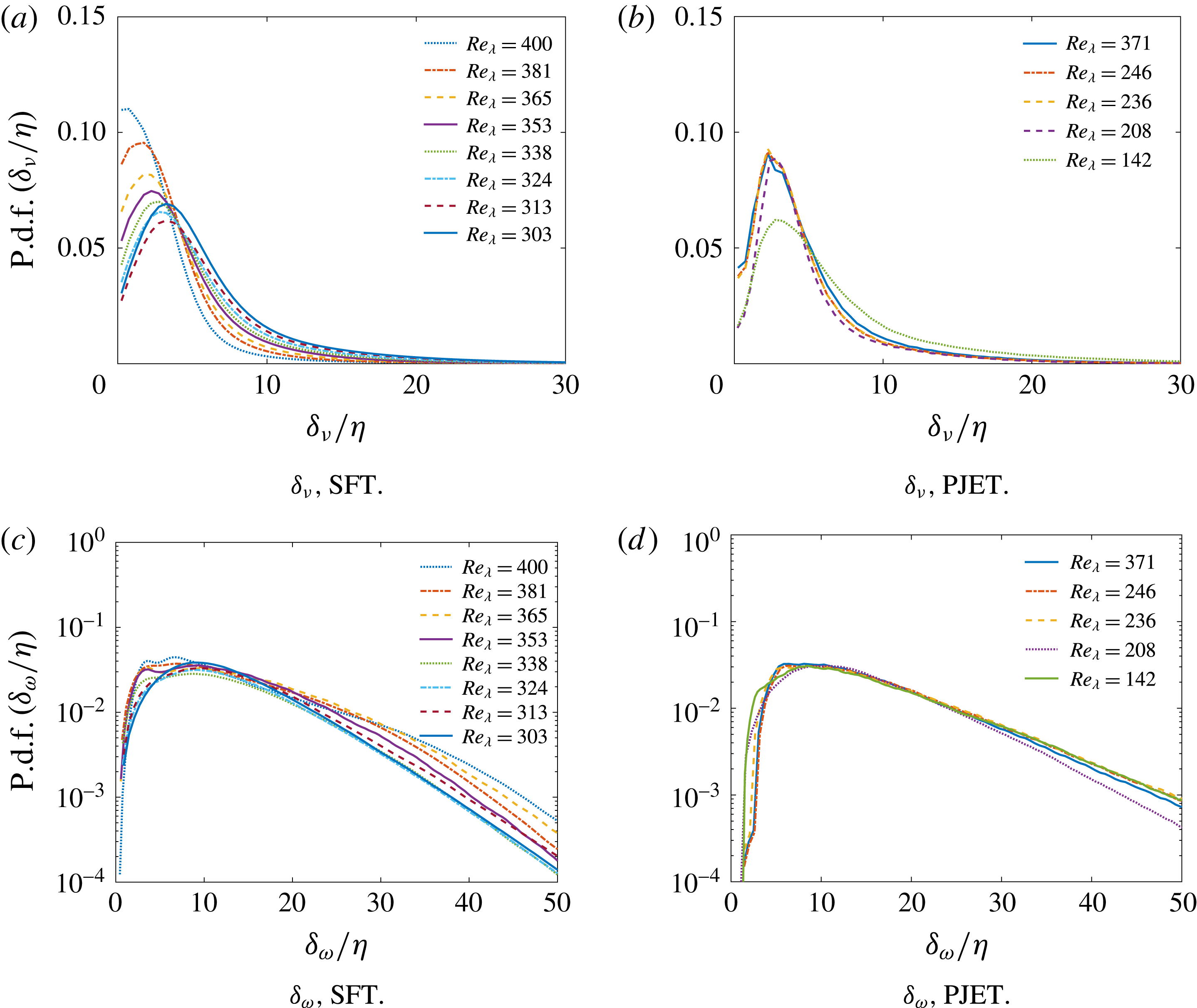
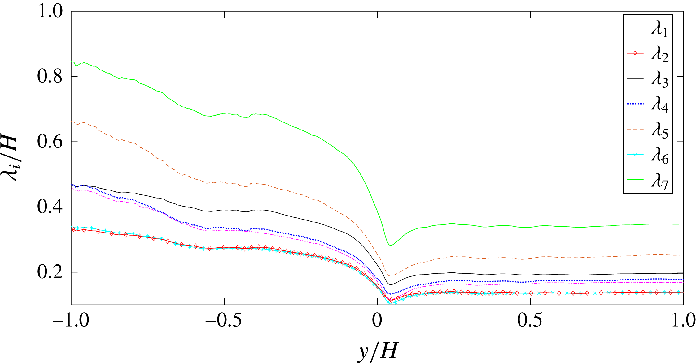
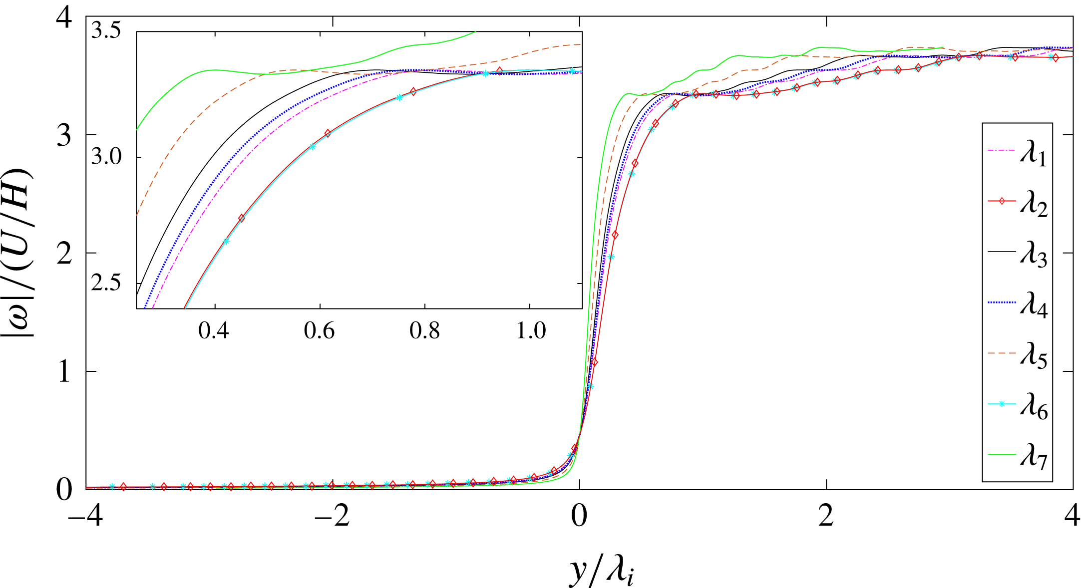
1 Introduction
The turbulent/non-turbulent interface (TNTI) is the sharp and highly contorted layer that exists at the edges of jets, wakes, mixing layers and boundary layers, separating the turbulent core from the irrotational flow region (Bisset, Hunt & Rogers Reference Bisset, Hunt and Rogers2002; Holzner et al. Reference Holzner, Liberzon, Nikitin, Kinzelbach and Tsinober2007; Westerweel et al. Reference Westerweel, Fukushima, Pedersen and Hunt2009). The importance of this layer stems from the significant transfers of mass, momentum and scalars (heat) that take place across its thickness, which renders its physical understanding crucial to a variety of environmental and engineering problems; for example, the flow dynamics near the TNTI governs the entrainment and mixing rates in turbulent reacting jets (da Silva et al. Reference da Silva, Hunt, Eames and Westerweel2014a ).
It is important to clarify from the outset that this TNTI (or interfacial layer as described in detail in da Silva et al. Reference da Silva, Hunt, Eames and Westerweel2014a ) is a layer with finite thickness (not a surface) connecting the irrotational and turbulent core regions, and it is clear that the flow within this layer is (strictly speaking) rotational. It has been established recently that the TNTI contains two sublayers within itself: (i) a viscous superlayer (VSL), whose existence was first hypothesised by Corrsin & Kistler (Reference Corrsin and Kistler1955) and where viscous effects dominate, and (ii) a turbulent sublayer (TSL), also named the ‘buffer layer’ (van Reeuwijk & Holzner Reference van Reeuwijk and Holzner2014; Borrell & Jiménez Reference Borrell and Jiménez2016), where inertial effects dominate. These two sublayers have a small but finite thickness which when added gives the total thickness of the TNTI, with the VSL being the outer part of the TNTI, while the TSL is in contact with the turbulent core region of the flow, e.g. the turbulent core of a mixing layer. Internal layers separating regions with different vorticity levels, as described in Ishihara, Kaneda & Hunt (Reference Ishihara, Kaneda and Hunt2013), have a different nature and will not be discussed here.
The scaling of the mean thickness of the TNTI
 $\langle \unicode[STIX]{x1D6FF}_{\unicode[STIX]{x1D714}}\rangle$
has been analysed in many works, where it has often been obtained by measuring the length scale of a characteristic vorticity jump observed at the TNTI. This is typically measured through conditional statistics of the enstrophy in relation to a fixed position within the TNTI – usually the irrotational boundary (IB) – which is the surface delimiting the outer boundary of the TNTI as defined in da Silva et al. (Reference da Silva, Hunt, Eames and Westerweel2014a
), Watanabe et al. (Reference Watanabe, Sakai, Nagata, Ito and Hayase2015), and which, as discussed in detail in da Silva, Taveira & Borrell (Reference da Silva, Taveira and Borrell2014b
), can be easily detected due to the sharpness of the TNTI layer.
The mean thickness of this layer has been shown to be of the order of the Taylor micro-scale
 $\langle \unicode[STIX]{x1D6FF}_{\unicode[STIX]{x1D714}}\rangle \approx \unicode[STIX]{x1D706}$
in wakes (Bisset et al.
Reference Bisset, Hunt and Rogers2002), round jets (Westerweel et al.
Reference Westerweel, Fukushima, Pedersen and Hunt2009; Gampert et al.
Reference Gampert, Narayanaswamy, Schaefer and Peters2013), mixing layers (Attili, Cristancho & Bisetti Reference Attili, Cristancho and Bisetti2014) and boundary layers (Chauhan, Philip & Marusic Reference Chauhan, Philip and Marusic2014; Borrell & Jiménez Reference Borrell and Jiménez2016).
 $\langle \unicode[STIX]{x1D6FF}_{\unicode[STIX]{x1D714}}\rangle \approx \unicode[STIX]{x1D706}$
is also supported by rapid-distortion theory (Carruthers & Hunt Reference Carruthers and Hunt1986). On the other hand experiments and direct numerical simulations (DNS) of turbulent fronts without mean shear – or shear free turbulence (SFT) – suggest that this thickness scales with the Kolmogorov micro-scale
 $\unicode[STIX]{x1D702}$
(Holzner et al.
Reference Holzner, Liberzon, Nikitin, Kinzelbach and Tsinober2007, Reference Holzner, Liberzon, Luthi, Nikitin, Kinzelbach and Tsinober2008).
This issue was systematically studied by da Silva & Taveira (Reference da Silva and Taveira2010), who compared TNTIs from turbulent planar jets (PJET) and shear free turbulence (SFT) for a wide range of Reynolds numbers, between
 $60\leqslant Re_{\unicode[STIX]{x1D706}}\leqslant 160$
, where
 $Re_{\unicode[STIX]{x1D706}}=u^{\prime }\unicode[STIX]{x1D706}/\unicode[STIX]{x1D708}$
is the Taylor based Reynolds number, defined with the streamwise velocity
 $u^{\prime }$
, Taylor micro-scale
 $\unicode[STIX]{x1D706}$
and kinematic viscosity
 $\unicode[STIX]{x1D708}$
. For the turbulent planar jet cases, mean thicknesses of the order
 $\unicode[STIX]{x1D706}$
were obtained, where
 $\unicode[STIX]{x1D6FF}_{\unicode[STIX]{x1D714}}$
is measured using the jump of the conditional mean
 $|\unicode[STIX]{x1D714}_{z}|$
profile. Specifically, they observed
 $0.41<\langle \unicode[STIX]{x1D6FF}_{\unicode[STIX]{x1D714}}\rangle /\unicode[STIX]{x1D706}<1.34$
and
 $7.4<\langle \unicode[STIX]{x1D6FF}_{\unicode[STIX]{x1D714}}\rangle /\unicode[STIX]{x1D702}<34.3$
in the PJET configuration, where it was noticed also that the mean thickness of the TNTI was close to the radius of the large-scale eddies neighbouring the TNTI. Using the Burgers vortex model to describe these eddies, one can explain different scaling laws depending on the mean shear acting upon the vortices, with
 $\langle \unicode[STIX]{x1D6FF}_{\unicode[STIX]{x1D714}}\rangle \sim \sqrt{\unicode[STIX]{x1D708}L/u^{\prime }}\sim \unicode[STIX]{x1D706}$
for a flow with mean shear, and
 $\langle \unicode[STIX]{x1D6FF}_{\unicode[STIX]{x1D714}}\rangle \sim \sqrt{\unicode[STIX]{x1D708}\unicode[STIX]{x1D706}/u^{\prime }}\sim \unicode[STIX]{x1D702}$
in the absence of mean shear, where
 $\unicode[STIX]{x1D702}$
is the Kolmogorov micro-scale and
 $L$
is the integral scale inside the turbulence core region (Hunt et al.
Reference Hunt, Eames, Westerweel, Davidson, Voropayev, Fernando and Braza2010). Thus, the ‘Reynolds number and the magnitude of the mean shear affect the TNTI thickness insofar as they define the radial dimension of the large vorticity structures near the interface’ (da Silva & Taveira Reference da Silva and Taveira2010).
However, since as the Reynolds number increases these eddies become more fragmented, which consequently decreases the mean thickness of the TNTI, suspicion arises about the validity of the previous results in very high Reynolds number configurations. It is noteworthy that almost all the existing works assessing this issue used experimental or numerical data with typically
 $Re_{\unicode[STIX]{x1D706}}\lesssim 100$
. An interesting exception is Chauhan et al. (Reference Chauhan, Philip and Marusic2014) (
 $Re_{\unicode[STIX]{x1D706}}\approx 340$
), which we will discuss below. Otherwise, in all the numerical works dealing with this problem the highest Reynolds number assessed (
 $Re_{\unicode[STIX]{x1D706}}\approx 160$
) corresponds to a single simulation from da Silva & Taveira (Reference da Silva and Taveira2010), who expressed that ‘assessment of very high Reynolds number flows should be pursued in future works’.
It is important to review in detail the actual values obtained for the mean thicknesses of the TNTI layer in several previous works. Bisset et al. (Reference Bisset, Hunt and Rogers2002) were the first to measure the mean thickness of the TNTI layer by using DNS of temporally evolving wakes. They defined the mean thickness as the vorticity jump obtained from conditional statistics in relation to the IB position and obtained a mean thickness in the range
 $0.06<\langle \unicode[STIX]{x1D6FF}_{\unicode[STIX]{x1D714}}\rangle /\unicode[STIX]{x1D6FF}_{0.5}<0.08$
, where
 $\unicode[STIX]{x1D6FF}_{0.5}$
is the half-width of the wake. They state that the mean thickness of the TNTI layer ‘is comparable to the Taylor micro-scale
 $\unicode[STIX]{x1D706}$
, but it is an order of magnitude larger than the Kolmogorov micro-scale’.
Both Eulerian and Lagrangian conditional profiles of the vorticity were also used in experiments and DNS of SFT carried out by Holzner et al. (Reference Holzner, Liberzon, Nikitin, Kinzelbach and Tsinober2007, Reference Holzner, Liberzon, Luthi, Nikitin, Kinzelbach and Tsinober2008). In this case the length/time scales associated with the enstrophy jump across the TNTI are only a few Kolmogorov scales
 $\langle \unicode[STIX]{x1D6FF}_{\unicode[STIX]{x1D714}}\rangle /\unicode[STIX]{x1D702}\approx 2$
; however, the Reynolds numbers used in these works (
 $Re_{\unicode[STIX]{x1D706}}=50$
) is too low to allow conclusions to be drawn for TNTIs at high Reynolds numbers. An interesting study by Wolf et al. (Reference Wolf, Holzner, Luthi, Krug, Kinzelbach and Tsinober2013) added experimental round jets with
 $Re_{D}=5000$
(corresponding to
 $Re_{\unicode[STIX]{x1D706}}=80$
) to assess the effects of mean shear in the mean thickness of the TNTI layer. They obtain
 $\langle \unicode[STIX]{x1D6FF}_{\unicode[STIX]{x1D714}}\rangle /\unicode[STIX]{x1D702}\approx 15$
for the case of a jet, which is considerably higher than in the lower Reynolds number of the SFT case.
Westerweel et al. (Reference Westerweel, Fukushima, Pedersen and Hunt2009) used experimental data from a round jet at Reynolds number
 $Re_{D}=U_{0}D/\unicode[STIX]{x1D708}=2000$
to generate conditional
 $\unicode[STIX]{x1D714}_{z}$
vorticity profiles. Defining the mean thickness of the TNTI using the vorticity jump in their figure 12 one has
 $\langle \unicode[STIX]{x1D6FF}_{\unicode[STIX]{x1D714}}\rangle /\unicode[STIX]{x1D6FF}_{0.5}\approx 0.2$
, which (again using estimates from Westerweel et al.
Reference Westerweel, Fukushima, Pedersen and Hunt2009) corresponds to
 $\langle \unicode[STIX]{x1D6FF}_{\unicode[STIX]{x1D714}}\rangle /\unicode[STIX]{x1D706}\approx 1.1$
.
Experimental results from round jets were also used by Khashehchi & Marusic (Reference Khashehchi and Marusic2013) for Reynolds numbers varying in the range
 $Re_{D}=U_{0}D/\unicode[STIX]{x1D708}=3000{-}6500$
. Conditional profiles of mean
 $\unicode[STIX]{x1D714}_{z}$
vorticity were again used to estimate the mean thickness of the TNTI layer. At
 $x/D=25$
they obtained
 $\langle \unicode[STIX]{x1D6FF}_{\unicode[STIX]{x1D714}}\rangle /\unicode[STIX]{x1D6FF}_{0.5}\approx 0.3$
which corresponds to
 $\langle \unicode[STIX]{x1D6FF}_{\unicode[STIX]{x1D714}}\rangle /\unicode[STIX]{x1D706}\approx 0.5$
and
 $\langle \unicode[STIX]{x1D6FF}_{\unicode[STIX]{x1D714}}\rangle /\unicode[STIX]{x1D702}\approx 6$
respectively. Experimental data from round jets at even higher Reynolds numbers were used by Gampert et al. (Reference Gampert, Narayanaswamy, Schaefer and Peters2013) (
 $Re_{D}=U_{0}D/\unicode[STIX]{x1D708}=3000{-}18\,440$
). They focused on the TNTI defined with the use of a passive scalar field with Schmidt number equal to
 $S_{c}=0.7$
. For axial positions in the range
 $10<x/D<30$
(corresponding to
 $60<Re_{\unicode[STIX]{x1D706}}<141$
) they observed that the mean thickness of the scalar interface scales as
 $\langle \unicode[STIX]{x1D6FF}_{\unicode[STIX]{x1D703}}\rangle /L\sim Re_{\unicode[STIX]{x1D706}}^{-1}$
, where
 $L$
is an estimated integral scale in the jet, which indicates that this layer scales with the Taylor micro-scale. However, as shown in Attili et al. (Reference Attili, Cristancho and Bisetti2014), the thickness of the scalar gradient is not a reliable metric for the thickness of the vorticity layer. Using DNS of spatially developing mixing layers, at a much higher Taylor based Reynolds number than in any of the previous works (
 $Re_{\unicode[STIX]{x1D706}}\approx 250$
) and by measuring the enstrophy jump in conditional profiles of
 $\unicode[STIX]{x1D714}_{z}$
vorticity, Attili et al. (Reference Attili, Cristancho and Bisetti2014) obtained
 $\langle \unicode[STIX]{x1D6FF}_{\unicode[STIX]{x1D714}}\rangle /\unicode[STIX]{x1D706}\approx 0.33$
and
 $\langle \unicode[STIX]{x1D6FF}_{\unicode[STIX]{x1D714}}\rangle /\unicode[STIX]{x1D702}\approx 14$
. This work is probably the first indication that something may be wrong with the supposed Taylor scaling of the TNTI layer because the mean thickness
 $\langle \unicode[STIX]{x1D6FF}_{\unicode[STIX]{x1D714}}\rangle /\unicode[STIX]{x1D706}$
is much smaller than in any previous works.
Experimental data from boundary layers were first used to measure the TNTI layer in Chauhan et al. (Reference Chauhan, Philip and Marusic2014). They use experimental data from four different boundary layers at different Reynolds numbers. Using the size of the shear layer thickness (associated with the spanwise vorticity
 $\unicode[STIX]{x1D714}_{z}$
) they estimate
 $0.5<\langle \unicode[STIX]{x1D6FF}_{\unicode[STIX]{x1D714}}\rangle /\unicode[STIX]{x1D706}<0.7$
and
 $11<\langle \unicode[STIX]{x1D6FF}_{\unicode[STIX]{x1D714}}\rangle /\unicode[STIX]{x1D702}<18$
. The closeness of these results to those of previous works suggests that the TNTI thickness in boundary layers should not be very different to TNTIs from shear free flows. Recently Borrell & Jiménez (Reference Borrell and Jiménez2016) have also analysed in detail the structure of the TNTI and have measured its thickness in a number of ways. All results consistently suggest that
 $\langle \unicode[STIX]{x1D6FF}_{\unicode[STIX]{x1D714}}\rangle /\unicode[STIX]{x1D706}\approx 1.0$
and
 $\langle \unicode[STIX]{x1D6FF}_{\unicode[STIX]{x1D714}}\rangle /\unicode[STIX]{x1D702}\approx 10$
, although they state that this scaling needs to be explained given the lack of mean shear influence at the TNTI location in boundary layers.
Finally, Watanabe and co-authors have consistently shown results which raise doubts about the supposed Taylor scaling of the TNTI at high Reynolds numbers. Using always the mean enstrophy jump obtained from conditional enstrophy profiles and using also Lagrangian statistics, they consistently show decreasing values of
 $\langle \unicode[STIX]{x1D6FF}_{\unicode[STIX]{x1D714}}\rangle /\unicode[STIX]{x1D706}$
as the Reynolds number increases, while
 $\langle \unicode[STIX]{x1D6FF}_{\unicode[STIX]{x1D714}}\rangle /\unicode[STIX]{x1D702}$
is very nearly constant with
 $\langle \unicode[STIX]{x1D6FF}_{\unicode[STIX]{x1D714}}\rangle /\unicode[STIX]{x1D702}\approx 10$
, independently of the Reynolds number. Specifically, DNS of spatially evolving planar jets at
 $Re_{H}=U_{0}H/\unicode[STIX]{x1D708}=2200$
(
 $Re_{\unicode[STIX]{x1D706}}=84$
at the jet centreline) give
 $\langle \unicode[STIX]{x1D6FF}_{\unicode[STIX]{x1D714}}\rangle /\unicode[STIX]{x1D706}\approx 0.6$
(Watanabe et al.
Reference Watanabe, Sakai, Nagata, Ito and Hayase2014), while DNS of mixing layers at
 $Re_{\unicode[STIX]{x1D6FF}}=380$
(
 $Re_{\unicode[STIX]{x1D706}}=99$
) show
 $\langle \unicode[STIX]{x1D6FF}_{\unicode[STIX]{x1D714}}\rangle /\unicode[STIX]{x1D702}\approx 10$
(Watanabe et al.
Reference Watanabe, Sakai, Nagata, Ito and Hayase2015). An impressive comparison is shown in Watanabe et al. (Reference Watanabe, da Silva, Sakai, Nagata and Hayase2016b
) and in Watanabe, Nagata & da Silva (Reference Watanabe, Nagata, da Silva and Perez-De-Tejada2017), where several mixing layers and planar jets at Reynolds numbers
 $105<Re_{\unicode[STIX]{x1D706}}<158$
have been used and where the mean thickness of the TNTI layer consistently gives
 $\langle \unicode[STIX]{x1D6FF}_{\unicode[STIX]{x1D714}}\rangle /\unicode[STIX]{x1D702}\approx 9{-}11$
. Watanabe et al. (Reference Watanabe, Riley, de Bruyn Kops, Diamessis and Zhou2016a
) showed also that in stably stratified wakes with Reynolds numbers
 $2700<Re_{L}<52\,000$
, the mean TNTI thickness is
 $\langle \unicode[STIX]{x1D6FF}_{\unicode[STIX]{x1D714}}\rangle /\unicode[STIX]{x1D702}\approx 15$
.
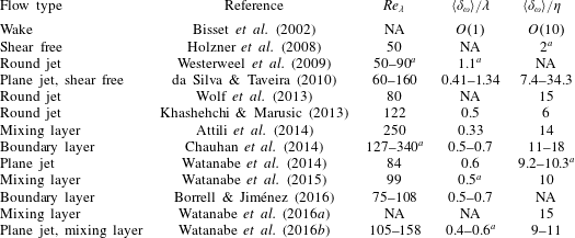
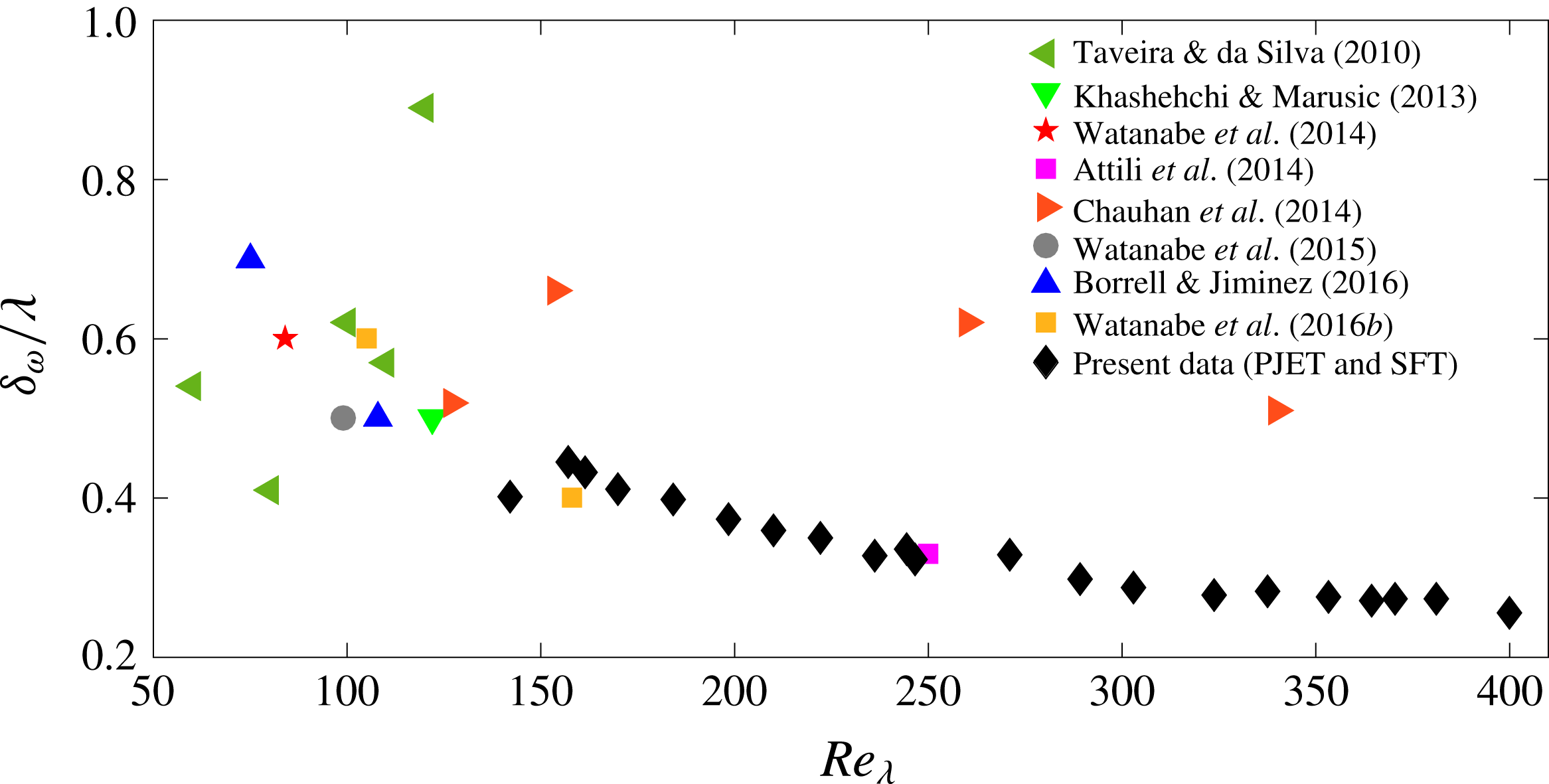
Table 1 summarises the values of
 $\langle \unicode[STIX]{x1D6FF}_{\unicode[STIX]{x1D714}}\rangle$
, normalised by
 $\unicode[STIX]{x1D706}$
and
 $\unicode[STIX]{x1D702}$
, obtained in several previous works. The majority of the existing data show
 $\langle \unicode[STIX]{x1D6FF}_{\unicode[STIX]{x1D714}}\rangle /\unicode[STIX]{x1D702}\approx 10$
and
 $\langle \unicode[STIX]{x1D6FF}_{\unicode[STIX]{x1D714}}\rangle /\unicode[STIX]{x1D706}\approx 0.5$
, and there are almost no cases with
 $\langle \unicode[STIX]{x1D6FF}_{\unicode[STIX]{x1D714}}\rangle /\unicode[STIX]{x1D706}=1$
. It is noteworthy that, with few exceptions, higher values of
 $Re_{\unicode[STIX]{x1D706}}$
tend to lead to smaller values of
 $\langle \unicode[STIX]{x1D6FF}_{\unicode[STIX]{x1D714}}\rangle /\unicode[STIX]{x1D706}$
. The comparison of the different values of
 $\langle \unicode[STIX]{x1D6FF}_{\unicode[STIX]{x1D714}}\rangle /\unicode[STIX]{x1D706}$
obtained in previous works is hampered by the different definitions of
 $\unicode[STIX]{x1D706}$
that have been used, and that can lead to errors of
 $50\,\%$
in
 $\langle \unicode[STIX]{x1D6FF}_{\unicode[STIX]{x1D714}}\rangle /\unicode[STIX]{x1D706}$
, as explained in appendix A.
Recall also that some authors define
 $\langle \unicode[STIX]{x1D6FF}_{\unicode[STIX]{x1D714}}\rangle$
using the jump in the conditional mean profile of
 $|\unicode[STIX]{x1D714}_{z}|$
(Westerweel et al.
Reference Westerweel, Fukushima, Pedersen and Hunt2009) while others use
 $|\unicode[STIX]{x1D714}|$
(Borrell & Jiménez Reference Borrell and Jiménez2016); however, as shown in several works (e.g. Attili et al.
Reference Attili, Cristancho and Bisetti2014),
 $\langle \unicode[STIX]{x1D6FF}_{\unicode[STIX]{x1D714}}\rangle$
obtained with the two definitions is similar. Interestingly, notwithstanding the small differences in the precise definitions used for
 $\langle \unicode[STIX]{x1D6FF}_{\unicode[STIX]{x1D714}}\rangle$
, table 1 shows that all available results point to approximately the same values of
 $\langle \unicode[STIX]{x1D6FF}_{\unicode[STIX]{x1D714}}\rangle /\unicode[STIX]{x1D706}$
and
 $\langle \unicode[STIX]{x1D6FF}_{\unicode[STIX]{x1D714}}\rangle /\unicode[STIX]{x1D702}$
, which indicates that there is something robust in the TNTI layer that emerges from all these (slightly different) definitions.
Summary of the mean values of the TNTI layer thickness
 $\langle \unicode[STIX]{x1D6FF}_{\unicode[STIX]{x1D714}}\rangle$
observed in several works, normalised by the Taylor
 $\unicode[STIX]{x1D706}$
and Kolmogorov
 $\unicode[STIX]{x1D702}$
micro-scales, respectively. Notice that as described in appendix A, the reference
 $\unicode[STIX]{x1D706}$
is computed using different definitions in different works, which complicates the comparison of the precise values of
 $\langle \unicode[STIX]{x1D6FF}_{\unicode[STIX]{x1D714}}\rangle /\unicode[STIX]{x1D706}$
obtained in several works.

a Estimated from the data in the corresponding reference.
In contrast, the mean thickness of the VSL
 $\langle \unicode[STIX]{x1D6FF}_{\unicode[STIX]{x1D708}}\rangle$
has been studied only recently (Taveira & da Silva Reference Taveira and da Silva2014) and was observed to be of the order of
 $\unicode[STIX]{x1D702}$
, and scaling with
 $\unicode[STIX]{x1D702}$
, as had been anticipated by Corrsin & Kistler (Reference Corrsin and Kistler1955). Specifically they obtained
 $3.3<\langle \unicode[STIX]{x1D6FF}_{\unicode[STIX]{x1D708}}\rangle /\unicode[STIX]{x1D702}<5.8$
. Similar values were recently obtained also by Watanabe et al. (Reference Watanabe, da Silva, Sakai, Nagata and Hayase2016b
) using DNS of planar jets and mixing layers, with
 $\langle \unicode[STIX]{x1D6FF}_{\unicode[STIX]{x1D708}}\rangle /\unicode[STIX]{x1D702}\approx 4$
. Bearing in mind that this layer drives the viscous diffusion of vorticity from the turbulent core into the irrotational region, by supposing that this mechanism is only controlled by the amount of vorticity inside the turbulent region
 $\unicode[STIX]{x1D714}^{\prime }$
and by the molecular viscosity of the fluid
 $\unicode[STIX]{x1D708}$
, from dimensional reasoning it follows that the mean VSL thickness should scale as
 $\langle \unicode[STIX]{x1D6FF}_{\unicode[STIX]{x1D708}}\rangle \sim \sqrt{\unicode[STIX]{x1D708}/\unicode[STIX]{x1D714}^{\prime }}\sim \unicode[STIX]{x1D702}$
. It is well known that the only way vorticity can be communicated into an irrotational flow region is by viscous diffusion. Since this is a viscous dominated process,
 $\unicode[STIX]{x1D708}$
should definitely be a part of quantities governing
 $\unicode[STIX]{x1D6FF}_{\unicode[STIX]{x1D708}}$
. Another question is whether the enstrophy being considered in the scaling above is the enstrophy from inside the turbulent core region. This assumption demands that (i) the enstrophy does not vary substantially from the turbulent core region until the VSL is reached, and (ii) that it stays approximately constant during the diffusion process, i.e. that the time scales of the viscous diffusion are much shorter than the time scales associated with temporal variations of vorticity from within the turbulent core region. Existing results for jets, wakes and mixing layers do support these two assumptions, e.g. the conditional profiles of enstrophy show that this quantity is roughly constant in almost all the turbulent core region, and only very close to the TNTI does the enstrophy start to decrease. This is very different to the situation observed in boundary layers, where the enstrophy displays maximum values very far away from the TNTI location and decreases continuously from the near-wall region to the TNTI location.
Can similar dimensional reasoning be used to establish the mean thickness of the TSL
 $\langle \unicode[STIX]{x1D6FF}_{\unicode[STIX]{x1D70E}}\rangle$
, without using the simple explanation based on the dynamics of the eddies near the IB? It has been repeatedly observed that in this TSL or ‘buffer layer’ the enstrophy is not in approximate equilibrium between production and dissipation, but is evolving from the end of the VSL until the typical value inside the turbulent core region is observed
 $\unicode[STIX]{x1D714}^{\prime }$
(Watanabe et al.
Reference Watanabe, da Silva, Sakai, Nagata and Hayase2016b
). Since enstrophy production is the dominating mechanism in this layer, one can estimate that the reference length scale here is
 $\unicode[STIX]{x1D6FF}_{\unicode[STIX]{x1D70E}}=\unicode[STIX]{x1D6FF}_{\unicode[STIX]{x1D70E}}(C_{\unicode[STIX]{x1D714}},P_{\unicode[STIX]{x1D714}})$
, where
 $C_{\unicode[STIX]{x1D714}}$
and
 $P_{\unicode[STIX]{x1D714}}$
are the typical magnitudes of the enstrophy variation and production, respectively. These can be estimated as
 $C_{\unicode[STIX]{x1D714}}\sim u_{\unicode[STIX]{x1D70E}}(\unicode[STIX]{x2202}\unicode[STIX]{x1D714}^{\prime }/\unicode[STIX]{x2202}n)$
and
 $P_{\unicode[STIX]{x1D714}}\sim \unicode[STIX]{x1D714}^{\prime }s_{\unicode[STIX]{x1D70E}}$
, where
 $u_{\unicode[STIX]{x1D70E}}$
and
 $s_{\unicode[STIX]{x1D70E}}$
are the typical velocity and strain dominating the TSL region (
 $n$
is the direction normal to the IB), and it follows that the length scale associated with the TSL is of the order of
 $\langle \unicode[STIX]{x1D6FF}_{\unicode[STIX]{x1D70E}}\rangle \sim u_{\unicode[STIX]{x1D70E}}/s_{\unicode[STIX]{x1D70E}}$
.
The scaling of
 $\langle \unicode[STIX]{x1D6FF}_{\unicode[STIX]{x1D70E}}\rangle$
now depends on the choice of the defining references for
 $u_{\unicode[STIX]{x1D70E}}$
and
 $s_{\unicode[STIX]{x1D70E}}$
. In situations such as at the beginning of the transition region in jets and wakes, where
 $u_{\unicode[STIX]{x1D70E}}\sim u^{\prime }$
and
 $s_{\unicode[STIX]{x1D70E}}\sim u^{\prime }/L$
, one has
 $\langle \unicode[STIX]{x1D6FF}_{\unicode[STIX]{x1D70E}}\rangle \sim L$
; for example, at the beginning of the transition to turbulence in a jet this layer scales with the jet radius. Further downstream, when the mean shear dominates the TNTI and
 $u_{\unicode[STIX]{x1D70E}}\sim u^{\prime }$
and
 $s_{\unicode[STIX]{x1D70E}}\sim u^{\prime }/\unicode[STIX]{x1D706}$
, one has
 $\langle \unicode[STIX]{x1D6FF}_{\unicode[STIX]{x1D70E}}\rangle \sim \unicode[STIX]{x1D706}$
. Even further downstream, or at very high Reynolds numbers, where the ‘linearities’ imposed by the presence of a mean shear, are not important compared to nonlinearities of turbulence,
 $u_{\unicode[STIX]{x1D70E}}\sim u_{\unicode[STIX]{x1D702}}$
and
 $s_{\unicode[STIX]{x1D70E}}\sim u_{\unicode[STIX]{x1D702}}/\unicode[STIX]{x1D702}$
, which yields
 $\langle \unicode[STIX]{x1D6FF}_{\unicode[STIX]{x1D70E}}\rangle \sim \unicode[STIX]{x1D702}$
.
The above reasoning has the big limitation that results from different scaling laws being obtained from different choices of
 $u_{\unicode[STIX]{x1D70E}}$
and
 $s_{\unicode[STIX]{x1D70E}}$
, and we cannot rule out the possibility that the scaling of the TNTI has absolutely nothing to do with the effects of mean shear, as discussed below. However, the above explanation is consistent with the results of da Silva & Taveira (Reference da Silva and Taveira2010), and is also consistent with results obtained from rapid-distortion theory, as shown in Carruthers & Hunt (Reference Carruthers and Hunt1986) and Teixeira & da Silva (Reference Teixeira and da Silva2012).
The goal of the present work is to establish the high Reynolds number scaling of the TNTI together with its two sublayers, the VSL and TSL, given the limited Reynolds numbers that have been used in the past to study this issue. For this purpose direct numerical simulations (DNS) of temporal planar jets (PJET) and shear free turbulence (SFT) have been carried out, with Reynolds numbers in the range
 $142\lesssim Re_{\unicode[STIX]{x1D706}}\lesssim 400$
. Unsurprisingly, the results show that the TNTI and all its sublayers scale with the Kolmogorov micro-scale, provided a threshold Reynolds number of
 $Re_{\unicode[STIX]{x1D706}}\gtrsim 200$
is attained. However, whereas the VSL is always of the order of the Kolmogorov micro-scale the TSL (and the TNTI) is approximately one order of magnitude larger than
 $\unicode[STIX]{x1D702}$
, where the scaling constant also reflects the characteristics of the intense vortices neighbouring the TNTI, being slightly larger for PJET than for SFT.
2 Direct numerical simulations of temporal planar jets and shear free turbulence
2.1 Numerical methods and computational parameters
The numerical simulations used in this work were carried out with a Navier–Stokes solver that uses classical pseudo-spectral methods (collocation method, Canuto et al.
Reference Canuto, Hussaini, Quarteroni and Zang1987) for spatial discretisation, and a third-order, tree-step Runge–Kutta scheme (Williamson Reference Williamson1980) for temporal advancement. This code is an upgraded version of the algorithm used in da Silva & Pereira (Reference da Silva and Pereira2008), the main difference being the decomposition of the computational domain for the message passing interface (MPI) library. Specifically, we use a two-dimensional pencil decomposition, which relies on the 2DECOMP&FFT library (http://2decomp.org) to handle the multi-core communication and three-dimensional Fourier transforms, providing excellent scalability to up to tens of thousands of cores. All the simulations were fully de-aliased using the
 $2/3$
rule.
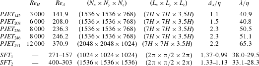
Several DNS of temporal turbulent planar jets were carried out which are similar to the simulations described in da Silva & Pereira (Reference da Silva and Pereira2008). The physical and computational parameters of the simulations are described in table 2. As in Stanley & Sarkar (Reference Stanley and Sarkar2000), Stanley, Sarkar & Mellado (Reference Stanley, Sarkar and Mellado2002) and da Silva & Pereira (Reference da Silva and Pereira2008), the initial conditions for the velocity field use a hyperbolic–tangent profile,
 $$\begin{eqnarray}\displaystyle & \displaystyle U(x,y,z)=\frac{U_{1}+U_{2}}{2}-\frac{U_{1}-U_{2}}{2}\tanh \left[\frac{H}{4\unicode[STIX]{x1D703}_{0}}\left(1-\frac{2|y|}{H}\right)\right], & \displaystyle\end{eqnarray}$$
where
 $\unicode[STIX]{x1D703}_{0}$
is the initial momentum thickness, and
 $U_{1}=1$
and
 $U_{2}=0$
, to which a three-component velocity fluctuating ‘spectral noise’ was superimposed by a convolution function that restricts the initial velocity noise to the initial shear layer region of the jet. The ratio between the initial momentum thickness (
 $\unicode[STIX]{x1D703}_{0}$
) and the jet initial slot-width
 $H$
is equal to
 $H/\unicode[STIX]{x1D703}_{0}=35$
, and the amplitude of spectral noise is 5 % of the maximum velocity in order to accelerate the transition to the turbulent regime and quickly attain a fully developed turbulent state, similarly to Stanley & Sarkar (Reference Stanley and Sarkar2000), Stanley et al. (Reference Stanley, Sarkar and Mellado2002) and da Silva & Pereira (Reference da Silva and Pereira2008).
Summary of the temporal planar jet (PJET) and shear free turbulence (SFT) simulations.
 $(N_{x}\times N_{y}\times N_{z})$
is the number of collocation points used for the
 $x$
,
 $y$
and
 $z$
directions, respectively, and
 $(L_{x}\times L_{y}\times L_{z})$
is the size of the computational domain in the same directions.
 $Re_{H}$
is the initial Reynolds number for the temporal jet simulations (for SFT the initial Reynolds numbers are
 $Re_{\unicode[STIX]{x1D706}}=300$
and
 $405$
) and
 $Re_{\unicode[STIX]{x1D706}}$
is the Reynolds number based on the Taylor micro-scale for the self-similar regime taken from the instantaneous field used in the conditional statistics.
 $\unicode[STIX]{x1D6E5}_{x}/\unicode[STIX]{x1D702}$
and
 $\unicode[STIX]{x1D706}/\unicode[STIX]{x1D702}$
are the resolution and the ratio between the Taylor and Kolmogorov micro-scales respectively. Notice that the reference values for
 $Re_{\unicode[STIX]{x1D706}}$
,
 $\unicode[STIX]{x1D702}$
and
 $\unicode[STIX]{x1D706}$
for all flows are taken from the turbulent core region, by using conditional means (profiles) at a distance of
 $y_{I}/\unicode[STIX]{x1D702}=300$
from the IB, where these quantities are approximately constant.

The simulations differ in the initial value of the Reynolds number which varies in the range
 $Re_{H}=\unicode[STIX]{x0394}UH/\unicode[STIX]{x1D708}=3000{-}12\,000$
, where
 $\unicode[STIX]{x1D6E5}U=U_{1}-U_{2}$
. The computational domain extends to
 $(L_{x},L_{y},L_{z})=(7H,7H,3.5H)$
along the streamwise
 $(x)$
, normal
 $(y)$
, and spanwise
 $(z)$
jet directions, respectively, and the simulations use
 $(N_{x}\times N_{y}\times N_{z})=(1536\times 1536\times 768)$
collocation points, except for the biggest simulation with
 $(N_{x}\times N_{y}\times N_{z})=(2048\times 2048\times 1024)$
. In all simulations the grid is uniform and isotropic in the three spatial directions (
 $\unicode[STIX]{x0394}x=\unicode[STIX]{x0394}y=\unicode[STIX]{x0394}z$
).
As in da Silva & Pereira (Reference da Silva and Pereira2008), extensive validation tests were undertaken and showed that the simulations are accurate at the large and small scales and are representative of a fully developed turbulent plane jet. By
 $T/T_{ref}\approx 24$
, where
 $T_{ref}=H/(2U_{1})$
the long-term self-similar regime has already been attained, as observed in the collapse of the mean velocity and Reynolds stresses profiles at different times, and the simulations were halted before the effect of the boundary conditions could be observed in the jet statistics.
At the long-term self-similar regime (where the analysis is carried out) the Reynolds number based on the Taylor micro-scale is equal to
 $Re_{\unicode[STIX]{x1D706}}=142,208,236$
,
 $246$
and
 $370.9$
, for simulations
 $PJET_{142}$
,
 $PJET_{208}$
,
 $PJET_{236}$
,
 $PJET_{246}$
and
 $PJET_{371}$
, respectively, and the resolution is equal to
 $\unicode[STIX]{x0394}x/\unicode[STIX]{x1D702}=1.1,1.8,2.3,2.3$
and
 $2.2$
(see table 2), while the jet half-width is in the range
 $0.75\leqslant \unicode[STIX]{x1D6FF}_{0.5}/H\leqslant 1.05$
for all the simulations.
Two shear free turbulence (SFT) simulations were carried out in a periodic box of size
 $2\unicode[STIX]{x03C0}\times 2\unicode[STIX]{x03C0}\times 2\unicode[STIX]{x03C0}$
with
 $1024^{3}$
(
 $SFT_{1}$
) and
 $1536^{3}$
(
 $SFT_{2}$
) collocation points, respectively. These simulations were pioneered in Perot & Moin (Reference Perot and Moin1995), and similar SFT simulations have been reported before, for example in da Silva & Taveira (Reference da Silva and Taveira2010), Taveira & da Silva (Reference Taveira and da Silva2014) and Cimarelli et al. (Reference Cimarelli, Cocconi, Frohnapfel and Angelis2015).
The initial turbulent field is issued from previously run DNS of forced homogeneous isotropic turbulence (HIT), using the forcing scheme by Alvelius (Reference Alvelius1999) with a peak forcing concentrated in the three wavenumbers centred at
 $k_{p}=2$
, and characterised by a Reynolds number of
 $Re_{\unicode[STIX]{x1D706}}=300$
(
 $SFT_{1}$
) and
 $Re_{\unicode[STIX]{x1D706}}=405$
(
 $SFT_{2}$
), respectively, with a resolution of
 $k_{max}\unicode[STIX]{x1D702}=1.5$
(
 $SFT_{1}$
) and
 $k_{max}\unicode[STIX]{x1D702}=1.48$
(
 $SFT_{2}$
), while the turbulence integral scale is
 $L=0.8$
(
 $SFT_{1}$
) and
 $L=1.2$
(
 $SFT_{2}$
), which is approximately
 $7.8$
(
 $SFT_{1}$
) and
 $5.2$
(
 $SFT_{2}$
) times smaller than the box size, and does not affect the development of the flow within the turbulent core region (several tests have shown that a minimum of
 $4$
times smaller than the box size is needed for this purpose).
The SFT simulations start with an initial transient (intermediate) simulation, where the initial velocity fields from the HIT are convoluted by a profile that essentially maintains the velocity of the HIT simulation in
 $-\unicode[STIX]{x03C0}/4\leqslant y\leqslant +\unicode[STIX]{x03C0}/4$
, while artificially setting to zero the velocity field in the region
 $|y|\geqslant \unicode[STIX]{x03C0}/4$
. As in Cimarelli et al. (Reference Cimarelli, Cocconi, Frohnapfel and Angelis2015), the convolution profile used in
 $SFT_{2}$
is similar to the hyperbolic tangent profile used in the PJET simulations so that the initial transition between the HIT and the
 $u_{i}(\boldsymbol{x},t)=0$
region is smooth, while in
 $SFT_{1}$
a sharp (top hat) convolution profile is used. As in Perot & Moin (Reference Perot and Moin1995), the time step is maintained very small during this intermediate simulation (approximately equal to
 $1/10$
of the one used in the HIT simulations).
The actual SFT simulations are then started from this initial condition where the initial isotropic turbulence fields spread into the irrotational region in the absence of mean shear, thereby developing two distinct (upper and lower) TNTI layers as the turbulence slowly decays within the core of the turbulent region. During the simulations the Reynolds number within the turbulent region decays from
 $Re_{\unicode[STIX]{x1D706}}=271{-}157$
(
 $SFT_{1}$
) and
 $Re_{\unicode[STIX]{x1D706}}=400{-}303$
(
 $SFT_{2}$
), respectively, while the resolution increases from
 $\unicode[STIX]{x0394}x/\unicode[STIX]{x1D702}=1.37{-}0.99$
(
 $SFT_{1}$
) and
 $\unicode[STIX]{x0394}x/\unicode[STIX]{x1D702}=1.33{-}1.13$
(
 $SFT_{2}$
). During each SFT the mean position of the two TNTIs moves from an initial region at
 $|y_{I}|\approx \unicode[STIX]{x03C0}/4$
into
 $|y_{I}|\approx \unicode[STIX]{x03C0}/2$
. When the simulations were halted no influence of the periodicity could be observed in any statistics. Table 2 summarises the details of the SFT simulations.
2.2 Conditional mean enstrophy profiles
Conditional statistics with respect to the distance from the TNTI have been used in several works (e.g. da Silva et al.
Reference da Silva, Hunt, Eames and Westerweel2014a
) and references therein, and are denoted here by
 $\langle \rangle _{I}$
. In the present work only a single instantaneous field is used (for each case) to compute the conditional statistics, since this is enough to obtain reasonably good convergence of almost all of the quantities of interest. Since all the flows are time-evolving, the turbulence reference quantities are taken from the turbulent core region of each particular instant/field. It was observed in previous works, e.g. Taveira & da Silva (Reference Taveira and da Silva2014) (and it has been confirmed again here), that for the case of the jet any field taken from the self-similar region is statistically equivalent in terms of the conditional statistics. The fact that the temporal nature of the flow does not affect the conditional statistics is explained by the fact that we are here analysing mainly small-scale quantities that quickly adjust to the (slow) variation of the large-scale quantities with time.
The procedure used to obtain these statistics follows roughly three steps: (i) the location of the outer edge of the TNTI – the irrotational boundary (IB) – is obtained; (ii) a local three-dimensional (3-D) axis is then placed with its origin at each of the
 $N_{x}\times N_{z}$
points from the upper and lower IB, with an axis (
 $y_{I}$
) pointing in the 3-D (
 $x,y,z$
) normal direction of the local outer boundary surface; (iii) the conditional statistics are then computed as a function of the distance
 $y_{I}$
to the TNTI layer using this (local) 3-D normal to the irrotational boundary surface. Notice that the conditional statistics use a finer grid than the original Navier–Stokes grid with four points per
 $\unicode[STIX]{x0394}x$
, and a trilinear interpolation. Previous tests using interpolation by splines showed virtually no difference in the conditional statistics, which indicates that the grid is sufficiently refined. It is also important to stress that as in many previous works (e.g. Westerweel et al.
Reference Westerweel, Fukushima, Pedersen and Hunt2009), bubbles of irrotational flow inside the turbulent region, as well as islands of turbulent flow in the irrotational region, are discarded from the statistical sample.
The IB is defined as the surface where the vorticity magnitude
 $(\unicode[STIX]{x1D714}_{i}\unicode[STIX]{x1D714}_{i})^{1/2}$
is equal to a certain threshold
 $\unicode[STIX]{x1D714}=\unicode[STIX]{x1D714}_{tr}$
, and marks a particular well-defined position within the TNTI as described in Watanabe et al. (Reference Watanabe, Sakai, Nagata, Ito and Hayase2015), where the threshold is obtained by quantifying the volume of the turbulent region as a function of
 $\unicode[STIX]{x1D714}_{tr}$
, as described in da Silva et al. (Reference da Silva, Hunt, Eames and Westerweel2014a
) and Watanabe et al. (Reference Watanabe, Sakai, Nagata, Ito and Hayase2015).
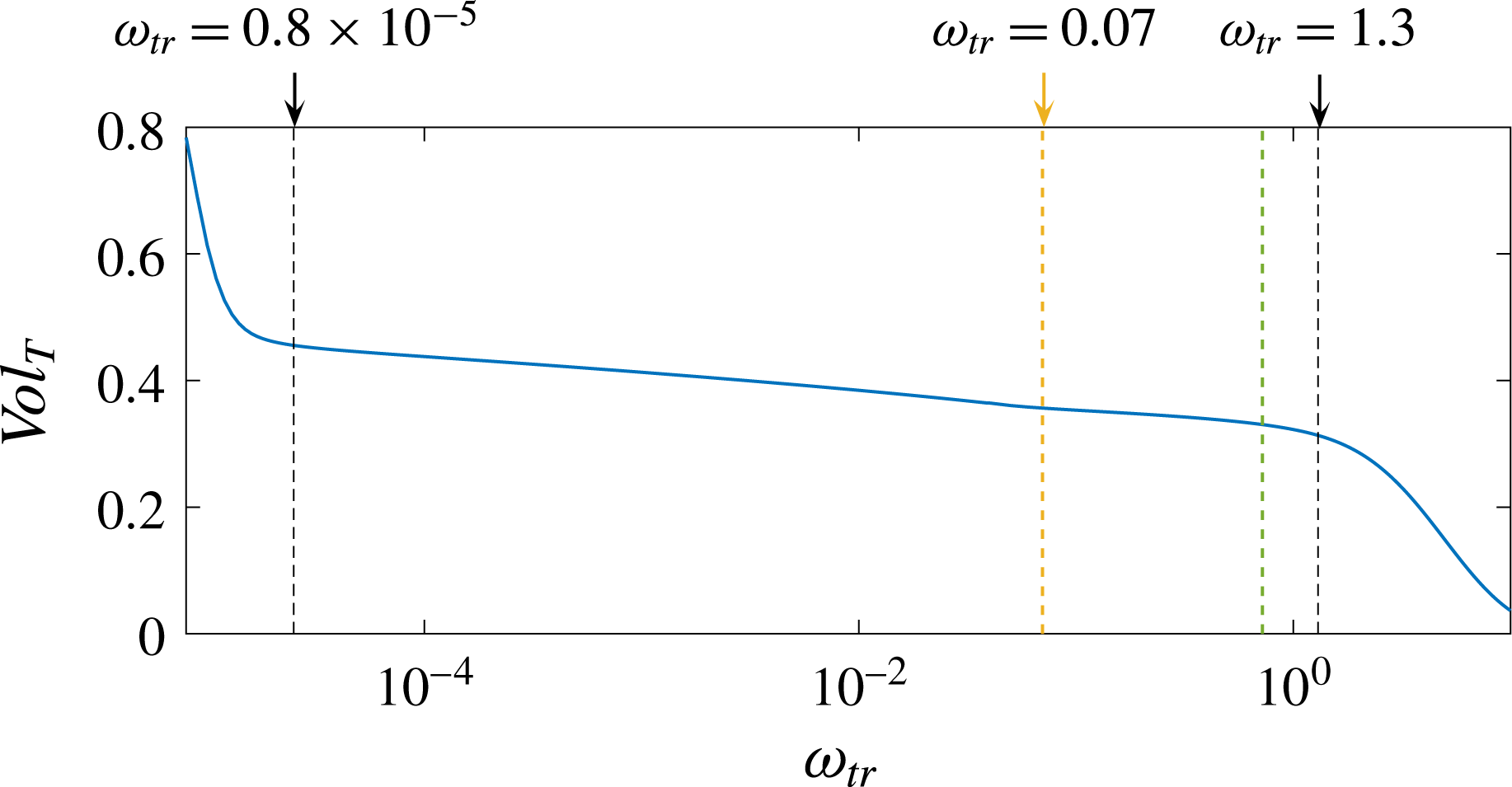
Figure 1 shows the turbulent volume
 $Vol_{T}(\unicode[STIX]{x1D714}_{tr})$
defined as the number of flow points where
 $\unicode[STIX]{x1D714}=(\unicode[STIX]{x1D714}_{i}\unicode[STIX]{x1D714}_{i})^{1/2}$
is above a given threshold
 $\unicode[STIX]{x1D714}_{tr}$
for
 $PJET_{246}$
. Similar plots have been obtained in other flow types, e.g. mixing layers and boundary layers, and using very different numerical schemes, e.g. spectral or finite differences (Taveira et al.
Reference Taveira, Diogo, Lopes and da Silva2013; Watanabe et al.
Reference Watanabe, Sakai, Nagata, Ito and Hayase2014; da Silva et al.
Reference da Silva, Taveira and Borrell2014b
; Watanabe et al.
Reference Watanabe, Sakai, Nagata, Ito and Hayase2015). Prior to the analysis of the IB position (and only for this purpose), a box filter with filter size
 $\unicode[STIX]{x1D6E5}/\unicode[STIX]{x0394}x=2$
was applied to the field of
 $(\unicode[STIX]{x1D714}_{i}\unicode[STIX]{x1D714}_{i})^{1/2}$
in order to smooth out some of the small-scale intermittency associated with this quantity, and to ease the automatic computation of
 $\unicode[STIX]{x1D714}_{tr}$
described below. Again, there is a ‘plateau’ in
 $Vol_{T}(\unicode[STIX]{x1D714}_{tr})$
corresponding to a range of values of
 $\unicode[STIX]{x1D714}_{th}$
for which
 $Vol_{T}$
changes very slowly, and which reflects the ‘sharpness’ of the TNTI and the fact that the IB position is relatively independent of this threshold (provided it is taken from this plateau where
 $Vol_{T}(\unicode[STIX]{x1D714}_{tr})$
changes slowly with
 $\unicode[STIX]{x1D714}_{tr}$
). The precise value of the threshold
 $\unicode[STIX]{x1D714}_{tr}$
used for each field is chosen by equating to zero the second derivative of
 $Vol_{T}(\unicode[STIX]{x1D714}_{tr})$
as in Taveira et al. (Reference Taveira, Diogo, Lopes and da Silva2013), Watanabe et al. (Reference Watanabe, Sakai, Nagata, Ito and Hayase2014), da Silva et al. (Reference da Silva, Taveira and Borrell2014b
) and Watanabe et al. (Reference Watanabe, Sakai, Nagata, Ito and Hayase2015). Specifically,
 $\unicode[STIX]{x1D714}_{tr}$
is chosen as the value
 $\unicode[STIX]{x1D714}$
for which
 $$\begin{eqnarray}\displaystyle & \displaystyle \frac{\unicode[STIX]{x2202}^{2}Vol_{T}(\unicode[STIX]{x1D714})}{\unicode[STIX]{x2202}\unicode[STIX]{x1D714}^{2}}\Big|_{\unicode[STIX]{x1D714}_{tr}}=0. & \displaystyle\end{eqnarray}$$
The robustness of this method to determine the IB position is attested by the fact that changing
 $\unicode[STIX]{x1D714}_{tr}$
between
 $\unicode[STIX]{x1D714}_{tr}=0.07$
and
 $\unicode[STIX]{x1D714}_{tr}=0.72$
causes the mean position of the IB (
 $Y_{IB}$
) to vary by only
 $\langle \unicode[STIX]{x0394}Y_{IB}\rangle /\unicode[STIX]{x1D702}=0.8$
.
Volume fraction of
 $\unicode[STIX]{x1D714}=(\unicode[STIX]{x1D714}_{i}\unicode[STIX]{x1D714}_{i})^{1/2}>\unicode[STIX]{x1D714}_{tr}$
as a function of
 $\unicode[STIX]{x1D714}_{tr}$
showing the lowest and highest possible threshold values for
 $PJET_{246}$
in a plateau with approximately constant
 $Vol_{T}$
. In the present case a threshold of
 $\unicode[STIX]{x1D714}_{tr}=0.72$
(green vertical line) was obtained, but any other values between the two limits has no effect on the conditional statistics, because the position of the IB is quite insensitive to
 $\unicode[STIX]{x1D714}_{tr}$
when it is taken from this plateau. In the present case the mean position of the IB changes by only
 $0.8\unicode[STIX]{x1D702}$
or
 $1.8\unicode[STIX]{x1D702}$
when
 $\unicode[STIX]{x1D714}_{tr}$
changes between
 $\unicode[STIX]{x1D714}_{tr}=0.07$
and
 $\unicode[STIX]{x1D714}_{tr}=0.72$
, and
 $\unicode[STIX]{x1D714}_{tr}=0.72$
and
 $\unicode[STIX]{x1D714}_{tr}=1.3$
, respectively.
 $\unicode[STIX]{x1D714}_{tr}>1.3$
is already slightly outside the plateau and cannot be taken as representative of the IB.

Some authors argue that using a physical definition would be more appropriate; however, in our opinion they fail to see that the issue of determining the IB is largely unphysically related, since it stems from the existence of experimental/numerical noise in the NT region that prevents the use of the only physical definition that should be used in this case, i.e. by simply defining the irrotational or non-turbulent (NT) and turbulent (T) regions with
 $\unicode[STIX]{x1D714}=0$
and
 $\unicode[STIX]{x1D714}\neq 0$
, respectively.
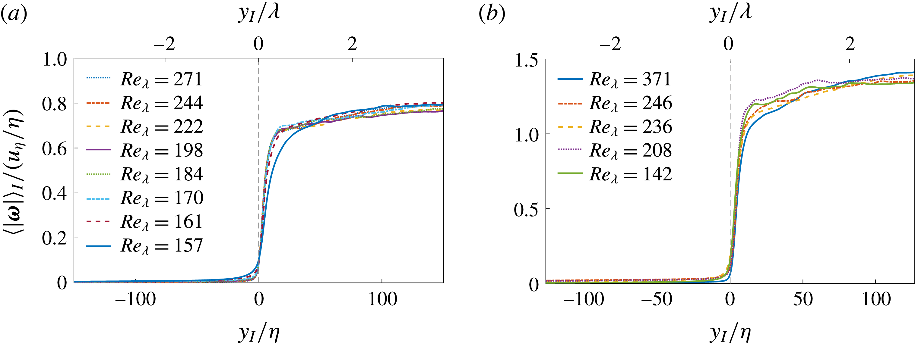
Figure 2(a,b) shows conditional mean profiles of enstrophy
 $|\unicode[STIX]{x1D74E}|=(\unicode[STIX]{x1D714}_{i}\unicode[STIX]{x1D714}_{i})^{1/2}$
, where
 $\unicode[STIX]{x1D714}_{i}=\unicode[STIX]{x1D700}_{ijk}\unicode[STIX]{x2202}u_{j}/\unicode[STIX]{x2202}x_{k}$
is the curl of the velocity field
 $u_{i}$
, for
 $SFT_{1}$
and all the PJET simulations used in the present work. The irrotational boundary is by definition located at
 $y_{I}=0$
, while the irrotational and turbulent regions are defined by
 $y_{I}<0$
and
 $y_{I}>0$
, respectively. The distance
 $y_{I}$
is normalised by the Kolmogorov micro-scale
 $\unicode[STIX]{x1D702}$
(and by the Taylor micro-scale
 $\unicode[STIX]{x1D706}$
, only for
 $Re_{\unicode[STIX]{x1D706}}=271$
in SFT and
 $Re_{\unicode[STIX]{x1D706}}=246$
in PJET), computed inside the turbulent region where their values are constant, i.e.
 $\unicode[STIX]{x1D702}=\unicode[STIX]{x1D702}\,(y_{I}\gg 0)$
and
 $\unicode[STIX]{x1D706}=\unicode[STIX]{x1D706}\,(y_{I}\gg 0)$
. Specifically, we take the reference values at
 $y_{I}/\unicode[STIX]{x1D702}=300$
from conditional mean profiles, where these and many other statistics are very nearly constant. The Taylor micro-scale is computed as
 $\unicode[STIX]{x1D706}=(\unicode[STIX]{x1D706}_{x}^{2}+\unicode[STIX]{x1D706}_{y}^{2}+\unicode[STIX]{x1D706}_{z}^{2})^{1/2}$
, with e.g.
 $\unicode[STIX]{x1D706}_{x}^{2}=2\langle {u^{\prime }}^{2}\rangle _{I}/\langle {(\text{d}u/\text{d}x)^{\prime }}^{2}\rangle _{I}$
, where
 $\langle {u^{\prime }}^{2}\rangle _{I}=\langle u^{2}\rangle _{I}-\langle u\rangle _{I}^{2}$
, and the conditional average is taken from inside the turbulent core region (i.e. at
 $y_{I}/\unicode[STIX]{x1D702}=300$
).
It is important to stress that the present procedure to compute the conditional statistics is essentially similar to the conditional statistics used in many previous works in the subject. Whereas da Silva & Pereira (Reference da Silva and Pereira2008) and Westerweel et al. (Reference Westerweel, Fukushima, Pedersen and Hunt2009) used 2-D normals, here we use 3-D normals in all the statistics, with no appreciable difference (for the lower Reynolds numbers). It is noteworthy, regarding for instance the observed mean TNTI thickness, that virtually all these previous works point to essentially the same values (for similar Reynolds numbers).
Conditional mean profiles of enstrophy
 $\langle |\unicode[STIX]{x1D74E}|\rangle _{I}$
in DNS of shear free turbulence (
 $SFT_{1}$
) and temporal planar jets (PJET), as a function of the distance from the TNTI
 $y_{I}$
, normalised by the Kolmogorov micro-scale
 $\unicode[STIX]{x1D702}$
where the reference turbulent quantities are computed using mean conditional profiles at
 $y_{I}/\unicode[STIX]{x1D702}=300$
(the axis in Taylor micro-scale units
 $\unicode[STIX]{x1D706}$
, is only for
 $Re_{\unicode[STIX]{x1D706}}=271$
in SFT (a) and for
 $Re_{\unicode[STIX]{x1D706}}=246$
in PJET (b)).

The enstrophy conditional profiles for
 $SFT_{1}$
(figure 2
a) normalised by the Kolmogorov velocity
 $u_{\unicode[STIX]{x1D702}}=(\unicode[STIX]{x1D708}\unicode[STIX]{x1D700})^{1/4}$
, and Kolmogorov micro-scale
 $\unicode[STIX]{x1D702}=(\unicode[STIX]{x1D708}^{3}/\unicode[STIX]{x1D700})^{1/4}$
(
 $\unicode[STIX]{x1D700}=2\unicode[STIX]{x1D708}s_{ij}s_{ij}$
is the viscous dissipation rate), and taken at different time instants with Reynolds numbers in the range
 $157\leqslant Re_{\unicode[STIX]{x1D706}}\leqslant 271$
approximately collapse in the same curve, except for the smaller Reynolds number corresponding to
 $Re_{\unicode[STIX]{x1D706}}=157$
. All the curves display a similar shape with a sharp increase in enstrophy across the TNTI followed by an approximately constant plateau in the turbulent region. The situation is similar for PJET where the conditional enstrophy profiles (figure 2
b) show approximate collapse for the higher Reynolds numbers.
A peak in
 $\langle |\unicode[STIX]{x1D714}_{z}|\rangle _{I}$
near the IB has been observed in some previous works (e.g. Bisset et al.
Reference Bisset, Hunt and Rogers2002; Westerweel et al.
Reference Westerweel, Fukushima, Pedersen and Hunt2009; da Silva & Taveira Reference da Silva and Taveira2010) and one may question if this feature can affect the shape of
 $\langle |\unicode[STIX]{x1D74E}|\rangle _{I}$
. This is suggested by the profiles of both
 $\langle |\unicode[STIX]{x1D74E}|\rangle _{I}$
and
 $\langle |\unicode[STIX]{x1D714}_{z}|\rangle _{I}$
obtained in several previous works (Bisset et al.
Reference Bisset, Hunt and Rogers2002; da Silva & Taveira Reference da Silva and Taveira2010). However, more recent results suggest that the impact of this
 $\langle |\unicode[STIX]{x1D714}_{z}|\rangle _{I}$
feature becomes less important at higher Reynolds numbers (e.g. Attili et al.
Reference Attili, Cristancho and Bisetti2014; Taveira & da Silva Reference Taveira and da Silva2014; Borrell & Jiménez Reference Borrell and Jiménez2016). The existence of a peak in
 $\langle |\unicode[STIX]{x1D714}_{z}|\rangle _{I}$
has been explained by the fact that vorticity cannot end within the fluid, and thus the axis of the intense vortices has to be tangent to the local TNTI position (da Silva, dos Reis & Pereira Reference da Silva, dos Reis and Pereira2011). Even if this is certainly true at any Reynolds number, the increasing complexity of the local vorticity field at high Reynolds numbers may cause this feature to be blurred. In the present results this feature is not observed.
The fact that the turbulent enstrophy value observed for the two flows is similar, with
 $\langle |\unicode[STIX]{x1D74E}|\rangle _{I}u_{\unicode[STIX]{x1D702}}/\unicode[STIX]{x1D702}~(y_{I}\gg 0)\approx 0.8$
in
 $SFT_{1}$
and
 $\langle |\unicode[STIX]{x1D74E}|\rangle _{I}u_{\unicode[STIX]{x1D702}}/\unicode[STIX]{x1D702}~(y_{I}\gg 0)\approx 1.2$
in PJET, also reflects a similar enstrophy dynamics within the turbulent region in the two flows, where as expected
 $\langle |\unicode[STIX]{x1D74E}|^{2}\rangle _{I}^{1/2}/(u_{\unicode[STIX]{x1D702}}/\unicode[STIX]{x1D702})\approx 1$
due to kinematic constraints.
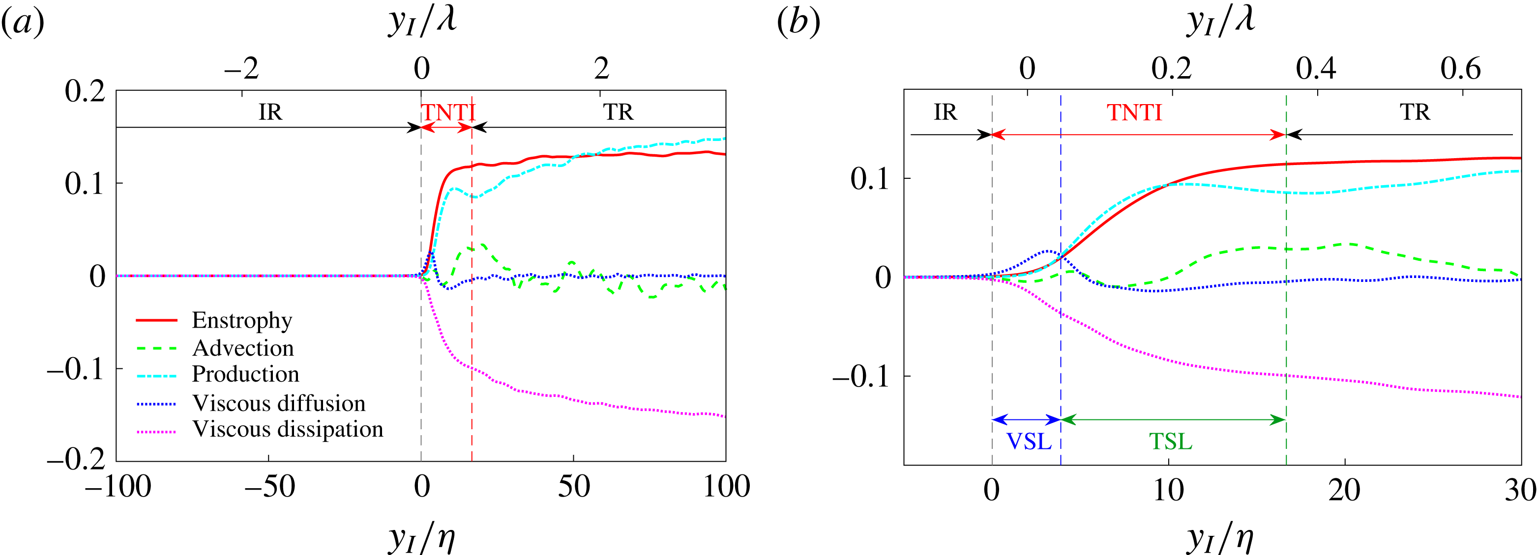
Conditional enstrophy and enstrophy budget for simulation
 $PJET_{246}$
, as a function of the distance to the TNTI
 $y_{I}$
, normalised by the Kolmogorov
 $\unicode[STIX]{x1D702}$
, and by the Taylor micro-scale
 $\unicode[STIX]{x1D706}$
, from (a)
 $-100\leqslant y_{I}/\unicode[STIX]{x1D702}\leqslant +100$
and (b)
 $-5\leqslant y_{I}/\unicode[STIX]{x1D702}\leqslant 30$
. The viscous superlayer (VSL) and turbulent sublayer (TSL) within the TNTI are also shown. IR and TR represent the irrotational, or non-turbulent (NT), and the turbulent (T) regions, respectively.

3 Results and discussion
3.1 The structure of the TNTI: the viscous superlayer and turbulent sublayer
Figure 3(a,b) shows the conditional enstrophy and the enstrophy budget for the simulation
 $PJET_{246}$
, which allows one to identify each one of the TNTI sublayers. Notice that the enstrophy budgets (and in particular the convective term) have to be computed taking into account the motion of the IB (as in Watanabe et al.
Reference Watanabe, Sakai, Nagata, Ito and Hayase2015). Except very close to the TNTI (
 $y_{I}\approx 0$
), the enstrophy dynamics is dominated by the enstrophy production
 $P_{\unicode[STIX]{x1D714}}=\unicode[STIX]{x1D714}_{i}\unicode[STIX]{x1D714}_{j}s_{ij}$
and viscous dissipation
 $E_{\unicode[STIX]{x1D714}}=-\unicode[STIX]{x1D708}(\unicode[STIX]{x2202}\unicode[STIX]{x1D714}_{i}/\unicode[STIX]{x2202}x_{j})^{2}$
, since all the other terms, i.e. enstrophy viscous diffusion
 $D_{\unicode[STIX]{x1D714}}=\unicode[STIX]{x1D708}\unicode[STIX]{x2202}^{2}/\unicode[STIX]{x2202}x_{j}\unicode[STIX]{x2202}x_{j}(\unicode[STIX]{x1D714}_{i}\unicode[STIX]{x1D714}_{i}/2)$
, and enstrophy convection
 $C_{\unicode[STIX]{x1D714}}=u_{j}\unicode[STIX]{x2202}/\unicode[STIX]{x2202}x_{j}(\unicode[STIX]{x1D714}_{i}\unicode[STIX]{x1D714}_{i}/2)$
, are negligible. The small oscillations in the advection for
 $y_{I}/\unicode[STIX]{x1D702}>30$
are certainly due to insufficient samples, but this constitutes no problem since, as shown here and in agreement with several previous works (Watanabe et al.
Reference Watanabe, Sakai, Nagata, Ito and Hayase2015), the convective term is smaller than the other terms across the entire TNTI layer, and moreover, is not used in the subsequent analysis of the TNTI layer. It may be connected to the small dip observed in the conditional profile of enstrophy production.
Figure 3(b) shows that moving from the irrotational (
 $y_{I}\ll 0$
) into the turbulent region (
 $y_{I}\gg 0$
), the initial growth of enstrophy across the TNTI (in
 $0\lesssim y_{I}/\unicode[STIX]{x1D702}\lesssim 4$
) is prompted by the enstrophy viscous diffusion, since the enstrophy production remains very low, while later (
 $4\lesssim y_{I}/\unicode[STIX]{x1D702}\lesssim 17$
) the enstrophy production dominates the budget, and the viscous diffusion becomes negligible. When the enstrophy ceases to grow and attains an approximate plateau, we have reached the turbulent core region (
 $y_{I}/\unicode[STIX]{x1D702}\gtrsim 17$
).
Similar conditional enstrophy budgets have been observed in TNTIs from very different flow types such as mixing layers (Watanabe et al. Reference Watanabe, da Silva, Sakai, Nagata and Hayase2016b ), plane wakes (Bisset et al. Reference Bisset, Hunt and Rogers2002), shear free turbulence (Holzner et al. Reference Holzner, Liberzon, Nikitin, Kinzelbach and Tsinober2007, Reference Holzner, Liberzon, Luthi, Nikitin, Kinzelbach and Tsinober2008; Taveira & da Silva Reference Taveira and da Silva2014) and boundary layers (Chauhan et al. Reference Chauhan, Philip and Marusic2014; Borrell & Jiménez Reference Borrell and Jiménez2016).
The TNTI (figure 3
b) is delimited by the irrotational region (IR) and by the turbulent core region (TR), and contains two adjacent sublayers defined by the relative importance between the enstrophy production and viscous diffusion: the viscous superlayer, with mean thickness
 $\langle \unicode[STIX]{x1D6FF}_{\unicode[STIX]{x1D708}}\rangle$
, is the sublayer within the TNTI where viscous diffusion dominates the growth of enstrophy, whereas the turbulent sublayer, with mean thickness
 $\langle \unicode[STIX]{x1D6FF}_{\unicode[STIX]{x1D70E}}\rangle$
, is the sublayer where enstrophy production outweighs viscous diffusion. Previous works on the TNTI simply defined the mean TNTI thickness
 $\langle \unicode[STIX]{x1D6FF}_{\unicode[STIX]{x1D714}}\rangle$
as the thickness associated with the enstrophy jump across the TNTI layer (e.g. Bisset et al.
Reference Bisset, Hunt and Rogers2002; Westerweel et al.
Reference Westerweel, Fukushima, Pedersen and Hunt2009; da Silva & Taveira Reference da Silva and Taveira2010), due to the difficulty of capturing the very fine VSL. In the present work the fine resolutions used allow us to actually measure these three layers simultaneously, i.e.
 $\unicode[STIX]{x1D6FF}_{\unicode[STIX]{x1D708}}$
and
 $\unicode[STIX]{x1D6FF}_{\unicode[STIX]{x1D714}}$
, while actually measuring the ‘true’ TSL thickness
 $\unicode[STIX]{x1D6FF}_{\unicode[STIX]{x1D70E}}$
for the first time.
In the next section we focus on the scaling of these two sublayers. The need to analyse the scaling of the two sublayers separately stems from the fact that they have a different nature, and because the scaling of one of them (the VSL) is consensual, while the other one is not. Studying both sublayers also allows for an easy comparison with results from previous works where only the total TNTI thickness has been computed (using the enstrophy).
The mathematical details of the present definitions of the several TNTI (sub)layers are given below, but as we will see, the (mean) thickness of the TNTI layer is similar (for similar Reynolds numbers) to the mean thicknesses previously observed in different flows using somewhat different definitions of the TNTI thicknesses. For example, Bisset et al. (Reference Bisset, Hunt and Rogers2002) used the conditional enstrophy jump, Westerweel et al. (Reference Westerweel, Fukushima, Pedersen and Hunt2009) used the conditional passive scalar jump, Chauhan et al. (Reference Chauhan, Philip and Marusic2014) used the conditional shear layer thickness and van Reeuwijk & Holzner (Reference van Reeuwijk and Holzner2014) used the entrainment velocity. In our opinion the agreement between the previous works can only be explained by the robustness or the universality of the main geometrical features of the TNTI in different flows. We believe that the present definition is a slight improvement over previous definitions because it includes information from the two (sub)layers within the TNTI layer and appropriated detection methods, designed to detect each one of the three boundaries defining their limits.
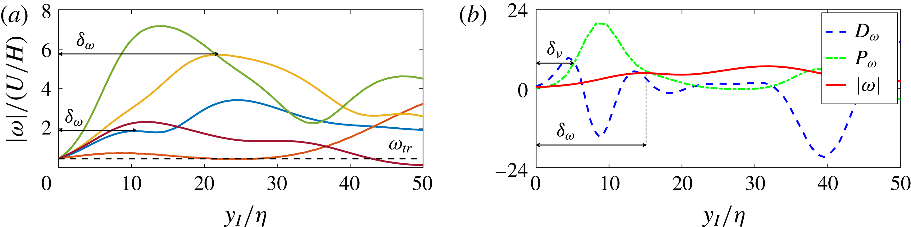
(a) Several local conditional profiles of vorticity magnitude observed in
 $PJET_{142}$
in the turbulent region (
 $y_{I}>0$
). The extent of the TNTI (
 $\unicode[STIX]{x1D6FF}_{\unicode[STIX]{x1D714}}$
) is defined as the distance between the IB and the first maximum of the vorticity magnitude. (b) Illustration of the determination of the local size of the VSL using two local conditional profiles of enstrophy production
 $P_{\unicode[STIX]{x1D714}}$
, and enstrophy diffusion
 $D_{\unicode[STIX]{x1D714}}$
. The extent of the VSL (
 $\unicode[STIX]{x1D6FF}_{\unicode[STIX]{x1D708}}$
) is defined as the distance between the IB and the point where the enstrophy production
 $P_{\unicode[STIX]{x1D714}}$
overcomes the enstrophy diffusion
 $D_{\unicode[STIX]{x1D714}}$
. The TSL (
 $\unicode[STIX]{x1D6FF}_{\unicode[STIX]{x1D70E}}$
) is locally defined as
 $\unicode[STIX]{x1D6FF}_{\unicode[STIX]{x1D70E}}=\unicode[STIX]{x1D6FF}_{\unicode[STIX]{x1D714}}-\unicode[STIX]{x1D6FF}_{\unicode[STIX]{x1D708}}$
.

3.2 Computation of the size of the TNTI and of its sublayers
In the present work the extent of the TNTI and its two sublayers was computed using the local conditional profiles. Figure 4(a) shows several local conditional profiles of vorticity magnitude in
 $PJET_{142}$
. Only the turbulent region is shown in this figure (
 $y_{I}>0$
) and each local conditional profile simply consists of the instantaneous vorticity magnitude obtained in a line which is locally normal (three-dimensional) to the IB. The local conditional vorticity typically rises from the IB (
 $y_{I}/\unicode[STIX]{x1D702}=0$
), where
 $\unicode[STIX]{x1D714}=\unicode[STIX]{x1D714}_{tr}$
, until a maximum is attained. As explained before, irrotational bubbles inside turbulent region are perceived as regions where the local vorticity magnitude becomes smaller than
 $\unicode[STIX]{x1D714}_{tr}$
, and these are discarded from the statistical sample. We define the local extent of the TNTI (
 $\unicode[STIX]{x1D6FF}_{\unicode[STIX]{x1D714}}$
) as the distance between the IB and this first local vorticity maximum,
 $$\begin{eqnarray}\displaystyle & \displaystyle \frac{\text{d}\langle \unicode[STIX]{x1D714}(\unicode[STIX]{x1D6FF}_{\unicode[STIX]{x1D714}})\rangle _{L}}{\text{d}y_{I}}=0, & \displaystyle\end{eqnarray}$$
where
 $\langle \rangle _{L}$
represents a local conditional profile.
Figure 4(b) shows typical local conditional profiles of enstrophy production
 $P_{\unicode[STIX]{x1D714}}$
and enstrophy diffusion
 $D_{\unicode[STIX]{x1D714}}$
, together with the vorticity magnitude
 $\unicode[STIX]{x1D714}=|\unicode[STIX]{x1D74E}|$
. Typically, the enstrophy diffusion rises to a maximum near the IB, and is latter followed by a rise in the enstrophy production. As in Taveira & da Silva (Reference Taveira and da Silva2014) we define the local extent of the VSL (
 $\unicode[STIX]{x1D6FF}_{\unicode[STIX]{x1D708}}$
) as the distance between the IB and the first point where the enstrophy production overcomes the enstrophy diffusion:
 $$\begin{eqnarray}\displaystyle & \displaystyle \langle \unicode[STIX]{x1D714}_{i}\unicode[STIX]{x1D714}_{j}s_{ij}(\unicode[STIX]{x1D6FF}_{\unicode[STIX]{x1D708}})\rangle _{L}=\left\langle \unicode[STIX]{x1D708}\frac{\unicode[STIX]{x2202}^{2}(\unicode[STIX]{x1D714}_{i}\unicode[STIX]{x1D714}_{i}/2)}{\unicode[STIX]{x2202}x_{j}\unicode[STIX]{x2202}x_{j}}(\unicode[STIX]{x1D6FF}_{\unicode[STIX]{x1D708}})\right\rangle _{L}. & \displaystyle\end{eqnarray}$$
Additionally, when the local enstrophy at this point is smaller than
 $\unicode[STIX]{x1D714}<\unicode[STIX]{x1D6FC}^{\unicode[STIX]{x1D708}}\unicode[STIX]{x1D714}_{tr}$
, where
 $\unicode[STIX]{x1D6FC}^{\unicode[STIX]{x1D708}}$
is an additional threshold used only for the VSL computation (with
 $\unicode[STIX]{x1D6FC}^{\unicode[STIX]{x1D708}}>1$
), these points are discarded. As in Taveira & da Silva (Reference Taveira and da Silva2014) this additional constraint was observed to be needed in order to obtain meaningful probability density functions for
 $\unicode[STIX]{x1D6FF}_{\unicode[STIX]{x1D708}}$
, and the particular value of the threshold used here is
 $\unicode[STIX]{x1D6FC}^{\unicode[STIX]{x1D708}}=2.9$
, which is very small compared to the typical values observed for the local conditional vorticity magnitude near the IB. For cases (local conditional profiles) where both
 $\unicode[STIX]{x1D6FF}_{\unicode[STIX]{x1D714}}$
and
 $\unicode[STIX]{x1D6FF}_{\unicode[STIX]{x1D708}}$
could be obtained, the local size of the TSL (
 $\unicode[STIX]{x1D6FF}_{\unicode[STIX]{x1D70E}}$
) is defined as
 $\unicode[STIX]{x1D6FF}_{\unicode[STIX]{x1D70E}}=\unicode[STIX]{x1D6FF}_{\unicode[STIX]{x1D714}}-\unicode[STIX]{x1D6FF}_{\unicode[STIX]{x1D708}}$
. Finally, the mean values of the thicknesses
 $\langle \unicode[STIX]{x1D6FF}_{\unicode[STIX]{x1D714}}\rangle$
,
 $\langle \unicode[STIX]{x1D6FF}_{\unicode[STIX]{x1D708}}\rangle$
and
 $\langle \unicode[STIX]{x1D6FF}_{\unicode[STIX]{x1D70E}}\rangle$
as well as their probability density functions (discussed below) were computed from the local values of
 $\unicode[STIX]{x1D6FF}_{\unicode[STIX]{x1D714}}$
,
 $\unicode[STIX]{x1D6FF}_{\unicode[STIX]{x1D708}}$
and
 $\unicode[STIX]{x1D6FF}_{\unicode[STIX]{x1D70E}}$
, respectively.
Many previous works have defined
 $\langle \unicode[STIX]{x1D6FF}_{\unicode[STIX]{x1D714}}\rangle$
by using the conditional mean enstrophy, whereas in the present work we compute
 $\langle \unicode[STIX]{x1D6FF}_{\unicode[STIX]{x1D714}}\rangle$
from the local
 $\unicode[STIX]{x1D6FF}_{\unicode[STIX]{x1D714}}$
, which is based on the local conditional profiles shown in figure 4(a). Notice, however, that exactly the same information is used in both cases, because both are based on the same local conditional profiles. In particular data points with
 $\unicode[STIX]{x1D714}<\unicode[STIX]{x1D714}_{tr}$
, e.g. when an irrotational bubble is detected inside the turbulent region, are discarded from the local conditional profiles, and therefore are not part of the conditional mean. Therefore, for the vorticity (or enstrophy) profiles, both contributions from points where a vortex is present, and also from gaps between vortices with lowed enstrophy levels, are equally included (provided
 $\unicode[STIX]{x1D714}>\unicode[STIX]{x1D714}_{tr}$
).
As remarked by an anonymous referee, strictly speaking the two procedures are not mathematically equal; however, as can be appreciated in appendices A and B, the result is very similar and the two procedures are equivalent. The present results are compared with the literature results in appendix B.
3.3 The mean thickness of the TNTI sublayers and their scaling
Figures 5(a–c) and 6(a–c) show the mean thickness of the VSL
 $\langle \unicode[STIX]{x1D6FF}_{\unicode[STIX]{x1D708}}\rangle$
, TSL
 $\langle \unicode[STIX]{x1D6FF}_{\unicode[STIX]{x1D70E}}\rangle$
and TNTI
 $\langle \unicode[STIX]{x1D6FF}_{\unicode[STIX]{x1D714}}\rangle$
, normalised by the Kolmogorov micro-scale
 $\unicode[STIX]{x1D702}$
, and the Taylor micro-scale
 $\unicode[STIX]{x1D706}$
, respectively, obtained as described above, for all the simulations used in the present work. Recall that at high Reynolds numbers the ratio between these two scales is
 $\unicode[STIX]{x1D702}/\unicode[STIX]{x1D706}\sim Re_{0}^{-1/4}\sim Re_{\unicode[STIX]{x1D706}}^{-1/2}$
(or
 $\unicode[STIX]{x1D706}/\unicode[STIX]{x1D702}\sim Re_{0}^{+1/4}\sim Re_{\unicode[STIX]{x1D706}}^{+1/2}$
), where
 $Re_{0}=u^{\prime }L/\unicode[STIX]{x1D708}$
is a macroscopic Reynolds number and
 $L$
is the integral scale of turbulence.
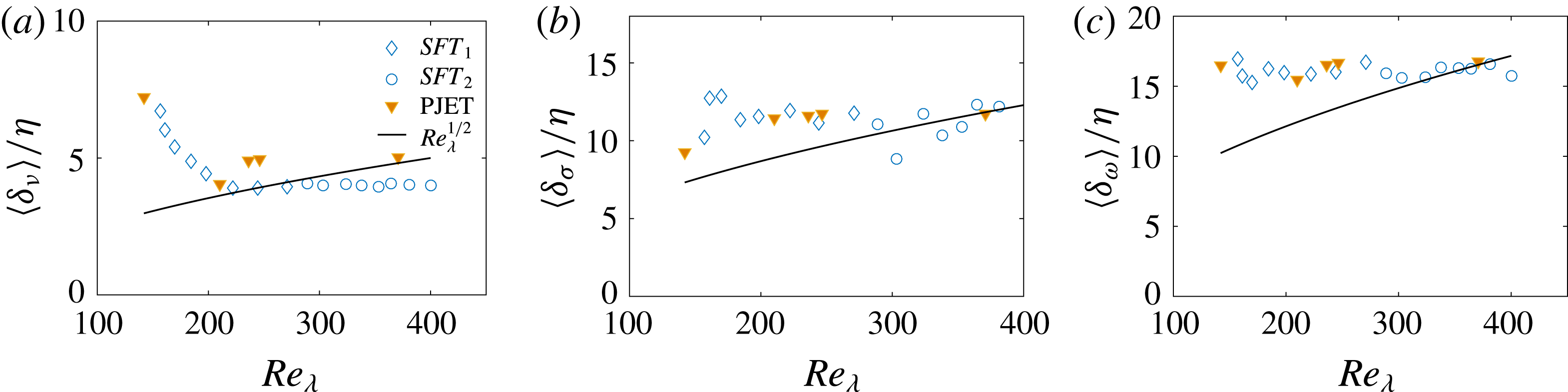
Mean thickness of the VSL (
 $\unicode[STIX]{x1D6FF}_{\unicode[STIX]{x1D708}}$
) (a), the TSL (
 $\unicode[STIX]{x1D6FF}_{\unicode[STIX]{x1D70E}}$
) (b) and TNTI (
 $\unicode[STIX]{x1D6FF}_{\unicode[STIX]{x1D714}}$
) (c) normalised by the Kolmogorov micro-scale
 $\unicode[STIX]{x1D702}$
as a function of the Reynolds number
 $Re_{\unicode[STIX]{x1D706}}$
, for the temporal turbulent planar jet (PJET) and shear free turbulence simulations (SFT).

Figure 5(a–c) shows that all the mean thicknesses of the VSL
 $\langle \unicode[STIX]{x1D6FF}_{\unicode[STIX]{x1D708}}\rangle$
, TSL
 $\langle \unicode[STIX]{x1D6FF}_{\unicode[STIX]{x1D70E}}\rangle$
and TNTI
 $\langle \unicode[STIX]{x1D6FF}_{\unicode[STIX]{x1D714}}\rangle$
tend to a constant value at high Reynolds numbers, when normalised by the Kolmogorov micro-scale
 $\unicode[STIX]{x1D702}$
. The panels also show that
 $\langle \unicode[STIX]{x1D6FF}_{\unicode[STIX]{x1D714}}\rangle >\langle \unicode[STIX]{x1D6FF}_{\unicode[STIX]{x1D70E}}\rangle >\langle \unicode[STIX]{x1D6FF}_{\unicode[STIX]{x1D708}}\rangle$
, as expected. The comparison of each one of the thicknesses with the scaling curve for
 $Re_{\unicode[STIX]{x1D706}}^{+1/2}$
clearly shows that neither of these quantities scales with the Taylor micro-scale at high Reynolds numbers. This is particularly clear for the TSL
 $\langle \unicode[STIX]{x1D6FF}_{\unicode[STIX]{x1D70E}}\rangle$
and TNTI
 $\langle \unicode[STIX]{x1D6FF}_{\unicode[STIX]{x1D714}}\rangle$
thicknesses, which have sometimes been associated with Taylor scaling, at lower Reynolds numbers. To clarify the scaling of the VSL, TSL and TNTI thicknesses, figure 6(a–c) shows the mean thicknesses of the VSL
 $\langle \unicode[STIX]{x1D6FF}_{\unicode[STIX]{x1D708}}\rangle$
, TSL
 $\langle \unicode[STIX]{x1D6FF}_{\unicode[STIX]{x1D70E}}\rangle$
and TNTI
 $\langle \unicode[STIX]{x1D6FF}_{\unicode[STIX]{x1D714}}\rangle$
, normalised by the Taylor micro-scale
 $\unicode[STIX]{x1D706}$
.
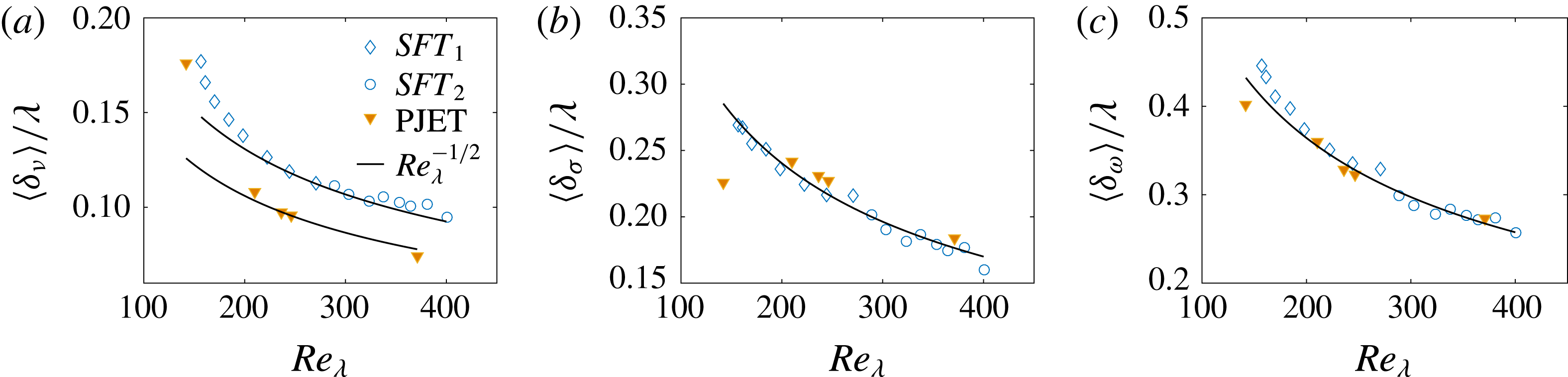
Mean thickness of the VSL (
 $\unicode[STIX]{x1D6FF}_{\unicode[STIX]{x1D708}}$
) (a), the TSL (
 $\unicode[STIX]{x1D6FF}_{\unicode[STIX]{x1D70E}}$
) (b) and TNTI (
 $\unicode[STIX]{x1D6FF}_{\unicode[STIX]{x1D714}}$
) (c) normalised by the Taylor micro-scale
 $\unicode[STIX]{x1D706}$
as a function of the Reynolds number
 $Re_{\unicode[STIX]{x1D706}}$
, for the temporal turbulent planar jet (PJET) and shear free turbulence simulations (SFT).

The first result observed from these curves is that none of the thicknesses is approximately equal to the Taylor micro-scale, e.g.
 $\langle \unicode[STIX]{x1D6FF}_{\unicode[STIX]{x1D714}}\rangle \neq \unicode[STIX]{x1D706}$
. Moreover, all of the mean thicknesses
 $\langle \unicode[STIX]{x1D6FF}\rangle$
show a consistent trend of decreasing
 $\langle \unicode[STIX]{x1D6FF}\rangle /\unicode[STIX]{x1D706}$
with increasing Reynolds number, and are always much smaller than
 $\unicode[STIX]{x1D706}$
, e.g.
 $0.16\leqslant \langle \unicode[STIX]{x1D6FF}_{\unicode[STIX]{x1D70E}}\rangle /\unicode[STIX]{x1D706}\leqslant 0.23$
for SFT. The highest obtained value is
 $\langle \unicode[STIX]{x1D6FF}_{\unicode[STIX]{x1D714}}\rangle /\unicode[STIX]{x1D706}\approx 0.45$
for the smallest Reynolds number case of the SFT simulations (
 $Re_{\unicode[STIX]{x1D706}}=157$
), which is comparable to the value of
 $\langle \unicode[STIX]{x1D6FF}_{\unicode[STIX]{x1D714}}\rangle /\unicode[STIX]{x1D706}\approx 0.57$
observed by da Silva & Taveira (Reference da Silva and Taveira2010) in a temporal planar turbulent jet starting from a turbulent channel flow DNS.
We start with the viscous superlayer thickness (figure 6
a) which is always much smaller than the Taylor micro-scale with
 $\langle \unicode[STIX]{x1D6FF}_{\unicode[STIX]{x1D708}}\rangle /\unicode[STIX]{x1D706}\leqslant 0.18$
, and for which no clear scaling can be discerned for lower Reynolds numbers
 $Re_{\unicode[STIX]{x1D706}}\lesssim 200$
for either PJET or SFT. Recall that this layer is responsible for the initial viscous communication of enstrophy into the irrotational flow region. For Reynolds numbers greater than
 $Re_{\unicode[STIX]{x1D706}}\approx 200$
, the ratio
 $\langle \unicode[STIX]{x1D6FF}_{\unicode[STIX]{x1D708}}\rangle /\unicode[STIX]{x1D706}$
closely follows the scaling law
 $\langle \unicode[STIX]{x1D6FF}_{\unicode[STIX]{x1D708}}\rangle /\unicode[STIX]{x1D706}\sim Re_{\unicode[STIX]{x1D706}}^{-1/2}$
, strongly suggesting a Kolmogorov scaling for this layer, i.e.
 $\langle \unicode[STIX]{x1D6FF}_{\unicode[STIX]{x1D708}}\rangle \sim \unicode[STIX]{x1D702}$
. Indeed the VSL is of the order of the Kolmogorov micro-scale with (for the higher Reynolds number cases
 $Re_{\unicode[STIX]{x1D706}}\gtrsim 200$
)
 $\langle \unicode[STIX]{x1D6FF}_{\unicode[STIX]{x1D708}}\rangle /\unicode[STIX]{x1D702}\approx 3.9$
(SFT) and
 $\langle \unicode[STIX]{x1D6FF}_{\unicode[STIX]{x1D708}}\rangle /\unicode[STIX]{x1D702}\approx 4.9$
(PJET). This result is not surprising since it has always been assumed that the VSL does indeed scale with
 $\unicode[STIX]{x1D702}$
due to its characteristic viscous dominated role. It is noteworthy that the mean values obtained here for low Reynolds numbers agree with those recently obtained by Taveira & da Silva (Reference Taveira and da Silva2014) at similar Reynolds numbers. In that work it was assumed that the VSL thickness could be explained by the dynamics of the intense vortices existing adjacent to the TNTI, but it is not clear if this simple explanation holds at the higher Reynolds numbers used in the present work (see below).
The mean TSL thickness (
 $\unicode[STIX]{x1D6FF}_{\unicode[STIX]{x1D70E}}$
) can be appreciated in figure 6(b), which displays together with figure 5(b) the first known results for this layer. Recall that the TSL is a region within the TNTI where viscous effects are no longer important; however, the flow has not yet reached a fully developed turbulent condition, since the enstrophy is rapidly increasing by nonlinear interactions between the enstrophy and strain (Holzner et al.
Reference Holzner, Liberzon, Nikitin, Kinzelbach and Tsinober2007). Again, excluding the lower Reynolds number case for the PJET (
 $Re_{\unicode[STIX]{x1D706}}=142$
), all the results closely follow a power law
 $\langle \unicode[STIX]{x1D6FF}_{\unicode[STIX]{x1D70E}}\rangle /\unicode[STIX]{x1D706}\sim Re_{\unicode[STIX]{x1D706}}^{-1/2}$
, and the observed values of the thicknesses are typically slightly larger than the VSL thicknesses with
 $10.4\leqslant \langle \unicode[STIX]{x1D6FF}_{\unicode[STIX]{x1D70E}}\rangle /\unicode[STIX]{x1D702}\leqslant 12.5$
for SFT and
 $11.5\leqslant \langle \unicode[STIX]{x1D6FF}_{\unicode[STIX]{x1D70E}}\rangle /\unicode[STIX]{x1D702}\leqslant 11.7$
for PJET, respectively for
 $Re_{\unicode[STIX]{x1D706}}\gtrsim 200$
(figure 5
b). The TSL is therefore larger than the VSL, but it also scales with the Kolmogorov micro-scale. Interestingly, the size of the TSL is roughly equal to the typical diameter
 $D_{ivs}$
of the intense vorticity structures existing inside the turbulent core region where typically
 $D_{ivs}\approx 10\unicode[STIX]{x1D702}$
(Jiménez & Wray Reference Jiménez and Wray1998; da Silva et al.
Reference da Silva, dos Reis and Pereira2011).
Finally, the mean thickness of the TNTI (
 $\unicode[STIX]{x1D6FF}_{\unicode[STIX]{x1D714}}$
) is analysed in figure 6(c). The values vary in the range
 $0.26\leqslant \langle \unicode[STIX]{x1D6FF}_{\unicode[STIX]{x1D714}}\rangle /\unicode[STIX]{x1D706}\leqslant 0.45$
for SFT and PJET, with the higher values obtained for the smaller Reynolds numbers. Unsurprisingly after the previous discussion, all the results closely display a power law
 $\langle \unicode[STIX]{x1D6FF}_{\unicode[STIX]{x1D714}}\rangle /\unicode[STIX]{x1D706}\sim Re_{\unicode[STIX]{x1D706}}^{-1/2}$
, while the observed values of the thicknesses are typically one order of magnitude greater than the Kolmogorov micro-scale with
 $15.6\leqslant \langle \unicode[STIX]{x1D6FF}_{\unicode[STIX]{x1D714}}\rangle /\unicode[STIX]{x1D702}\leqslant 16.8$
for SFT and
 $15.5\leqslant \langle \unicode[STIX]{x1D6FF}_{\unicode[STIX]{x1D70E}}\rangle /\unicode[STIX]{x1D702}\leqslant 16.7$
for PJET, respectively for
 $Re_{\unicode[STIX]{x1D706}}\gtrsim 200$
(figure 5
c). Thus the mean thickness of the TNTI is one order of magnitude bigger than the Kolmogorov micro-scale, although it also scales with the Kolmogorov micro-scale.
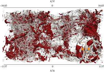
Top view of the upper shear layer for simulation
 $PJET_{371}$
showing the large vorticity structures (LVS) identified through low pressure iso-surfaces (dark/red), and the (small) intense vorticity structures (IVS) identified through iso-surfaces of
 $Q>0$
(white/grey), under the TNTI. The coordinates of the streamwise direction are normalised with the Kolmogorov micro-scale and Taylor scale, computed for this instant at the turbulent core region. The inset shows a zoom of the flow structures indicating the diameter (
 $9.8\unicode[STIX]{x1D702}$
) of one of the IVS.

As described in the introduction from da Silva & Taveira (Reference da Silva and Taveira2010), it was argued that
 $\langle \unicode[STIX]{x1D6FF}_{\unicode[STIX]{x1D714}}\rangle$
is imposed by the size of the vortices bounding the IB, themselves being controlled by the strain acting near the TNTI, which potentially leads into different scaling laws for PJET (
 $\unicode[STIX]{x1D6FF}_{\unicode[STIX]{x1D714}}\sim \unicode[STIX]{x1D706}$
) and SFT (
 $\unicode[STIX]{x1D6FF}_{\unicode[STIX]{x1D714}}\sim \unicode[STIX]{x1D702}$
). Note that the mean thicknesses
 $\langle \unicode[STIX]{x1D6FF}_{\unicode[STIX]{x1D714}}\rangle$
obtained in da Silva & Taveira (Reference da Silva and Taveira2010), where the Reynolds number varies within
 $60\leqslant Re_{\unicode[STIX]{x1D706}}\leqslant 160$
, do agree very well with the smaller Reynolds number cases used in the present work,
 $Re_{\unicode[STIX]{x1D706}}=157$
for SFT and
 $Re_{\unicode[STIX]{x1D706}}=142$
for PJET, respectively. However, for higher Reynolds numbers (
 $Re_{\unicode[STIX]{x1D706}}\geqslant 200$
) the present results clearly point to
 $\unicode[STIX]{x1D6FF}_{\unicode[STIX]{x1D714}}\sim \unicode[STIX]{x1D702}$
, for both SFT and PJET. This is easy to explain since ‘in the far field of a very high Reynolds number free shear flow the large vorticity structures (LVS) tend to be more fragmented and
 $\unicode[STIX]{x1D6FF}_{\unicode[STIX]{x1D714}}$
may approach the radius of the (small) intense vorticity structures (IVS),
 $\unicode[STIX]{x1D6FF}_{\unicode[STIX]{x1D714}}\sim \unicode[STIX]{x1D702}$
’ (da Silva & Taveira Reference da Silva and Taveira2010). Indeed, this seems to be the case as we now look into iso-surfaces of positive
 $Q$
, where
 $Q$
is the second invariant of the velocity gradient tensor (Martín et al.
Reference Martín, Ooi, Chong and Soria1998) and iso-surfaces of low pressure, both displayed in figure 7, showing the eddy structures near the TNTI for the higher Reynolds number PJET simulation. It is clear that unlike in da Silva & Taveira (Reference da Silva and Taveira2010), neither the pressure nor the
 $Q>0$
iso-surfaces show structures which could be confused with the classical Kelvin–Helmholtz vortices that arise during the transition to turbulence phase. On the contrary, both the large-scale and small-scale eddies are already too fragmented to exhibit a clear spatial orientation, and in particular the intense small-scale structures very much resemble the typical lack of preferred orientation observed in the ‘worms’ that are found in isotropic turbulence. In other words, even in the PJET simulations, for Reynolds numbers
 $Re_{\unicode[STIX]{x1D706}}\geqslant 200$
the eddies bordering the TNTI are ‘closer’ to those observed in SFT and it is not surprising that the same scaling (
 $\unicode[STIX]{x1D6FF}_{\unicode[STIX]{x1D714}}\sim \unicode[STIX]{x1D702}$
) should be observed for both SFT and PJET. Notice however that the ‘scaling constant’ is typically one order of magnitude larger than
 $\unicode[STIX]{x1D702}$
, roughly
 ${\approx}10\unicode[STIX]{x1D702}$
, approximately the diameter of the ‘worms’ observed in turbulent flows. The thickness of the TSL is therefore one order of magnitude greater than the thickness of the VSL, which is consistent with the fact that the TSL (unlike the VSL) is not dominated by viscous effects. It is interesting to recall the results obtained by Chauhan et al. (Reference Chauhan, Philip and Marusic2014) using experimental data from turbulent boundary layers at high Reynolds numbers. As remarked by an anonymous referee their figure 8(c) shows at least one measured interface thickness with
 $\unicode[STIX]{x1D6FF}_{\unicode[STIX]{x1D714}}/\unicode[STIX]{x1D702}\approx 10$
, thus anticipating the present results.
If this argument is correct, the same result (
 $\unicode[STIX]{x1D6FF}_{\unicode[STIX]{x1D714}}\sim \unicode[STIX]{x1D702}$
) would be observed in TNTIs from boundary layers at sufficiently high Reynolds numbers, because in that case the TNTI is located in a region with essentially no mean shear, in contrast with the case of the jet. The results for a boundary layer obtained in Chauhan et al. (Reference Chauhan, Philip and Marusic2014) described above seem to support this argument and the present results; however, before this issue is analysed in detail in other flows, e.g. wakes and boundary layers, one cannot rule out the possibility that the TNTIs from boundary layers may scale differently.
It is also possible that scaling of the TNTI has absolutely nothing to do with the effects of mean shear. Indeed, Elsinga et al. (Reference Elsinga, Ishihara, Goudar, da Silva and Hunt2017) showed that the structure of the turbulent motions, as reflected in the strain and vorticity fields, is only completely established for
 $Re_{\unicode[STIX]{x1D706}}\gtrsim 200{-}250$
, i.e. there is a ‘threshold/critical’ Reynolds number, much higher than the typically used
 $Re_{\unicode[STIX]{x1D706}}\approx 100$
(where the dissipation law holds), below which the turbulent motions are not yet characteristic of fully developed turbulence. This may explain why only above
 $Re_{\unicode[STIX]{x1D706}}\gtrsim 200$
do we observe the correct scaling laws for the TNTI thickness.
Yet another explanation for the scaling
 $\langle \unicode[STIX]{x1D6FF}_{\unicode[STIX]{x1D714}}\rangle \sim \unicode[STIX]{x1D702}$
observed here can possibly be given by the recent investigation of turbulent wakes carried out by Zhou & Vassilicos (Reference Zhou and Vassilicos2017). By considering zones with (classical) equilibrium dissipation and of non-equilibrium dissipation, both known to be present in the far field and in the near field of wakes, respectively, they infer that a scaling of
 $\langle \unicode[STIX]{x1D6FF}_{\unicode[STIX]{x1D714}}\rangle \sim \unicode[STIX]{x1D706}$
should be observed in the near field of turbulent wakes, whereas in the far field one should have
 $\langle \unicode[STIX]{x1D6FF}_{\unicode[STIX]{x1D714}}\rangle \sim \unicode[STIX]{x1D702}$
. This would suggest that the present high Reynolds number jets would fit into this second category, whereas the previous data observed at smaller Reynolds numbers would be similar to the near field of jets and mixing layers.
In their investigation Zhou & Vassilicos (Reference Zhou and Vassilicos2017) do not directly measure the value of the local thickness
 $\unicode[STIX]{x1D6FF}_{\unicode[STIX]{x1D714}}$
but infer its magnitude by using the viscosity and the characteristic velocity scale within the VSL. Unfortunately, only
 $\unicode[STIX]{x1D6FF}_{\unicode[STIX]{x1D708}}$
(but not
 $\unicode[STIX]{x1D6FF}_{\unicode[STIX]{x1D714}}$
) relates to the flow dynamics in the VSL, and moreover, no known results exist attesting the existence of non-equilibrium dissipation regions in jets. Therefore, although it is interesting to see that their analysis is consistent with Kolmogorov scaling observed in the present results, it is not clear how their explanations could be used in the present case.
Probability density functions (PDFs) of the local VSL thickness
 $\unicode[STIX]{x1D6FF}_{\unicode[STIX]{x1D708}}$
(a,b) and local TNTI thickness
 $\unicode[STIX]{x1D6FF}_{\unicode[STIX]{x1D714}}$
(c,d) normalised by the Kolmogorov micro-scale for the shear free turbulence (
 $SFT_{2}$
) and planar jet (PJET) simulations. The PDFs for
 $\unicode[STIX]{x1D6FF}_{\unicode[STIX]{x1D708}}$
are shown in linear–linear scale, whereas the PDFs for
 $\unicode[STIX]{x1D6FF}_{\unicode[STIX]{x1D714}}$
use linear–logarithmic scale.

3.4 The local thickness of the TNTI sublayers and their scaling
We now turn into the local scaling of
 $\unicode[STIX]{x1D6FF}_{\unicode[STIX]{x1D708}}$
,
 $\unicode[STIX]{x1D6FF}_{\unicode[STIX]{x1D70E}}$
and
 $\unicode[STIX]{x1D6FF}_{\unicode[STIX]{x1D714}}$
which can be investigated by the analysis of their probability density functions (PDFs), where each thickness is computed as defined before, but using the instantaneous conditional profiles that are obtained at each IB point along the TNTI. From now on we focus mainly on the results obtained for Reynolds numbers
 $Re_{\unicode[STIX]{x1D706}}\gtrsim 200$
, since the previous results suggest that the correct scaling of the TNTI layers may not be visible at smaller Reynolds numbers.
Figure 8(a,b) shows the PDFs of
 $\unicode[STIX]{x1D6FF}_{\unicode[STIX]{x1D708}}$
for SFT and PJET, respectively, in linear–linear scale. Except for the initial three instants (higher Reynolds numbers) from
 $SFT_{2}$
(where transient effects may still be present) the curves for the two flows exhibit a similar shape, with a distinctive peak associated with the maximum probability, followed by a smooth curve associated with much smaller probability values. Thus the majority of the values of
 $\unicode[STIX]{x1D6FF}_{\unicode[STIX]{x1D708}}$
come from a relatively small range of values. The maximum probability values obtained for all the simulations vary in the range
 $2.5\leqslant \unicode[STIX]{x1D6FF}_{\unicode[STIX]{x1D708}}/\unicode[STIX]{x1D702}\leqslant 3.4$
(for
 $Re_{\unicode[STIX]{x1D706}}\gtrsim 200$
). Taveira & da Silva (Reference Taveira and da Silva2014) observed large local values of
 $\unicode[STIX]{x1D6FF}_{\unicode[STIX]{x1D708}}$
to be associated with the presence of bigger intense vortices near the TNTI. It is however possible that this association is less distinct at higher Reynolds numbers, because the larger-scale structures will have the tendency to be more fragmented and to be less ‘coherent’, which explains why the location of the observed peaks does not change much for the higher Reynolds number cases. Conversely, at low Reynolds numbers, where the large-scale eddies tend to be larger, a more important contribution to the VSL statistics will come from events taking place at the periphery of these large eddies, and therefore one would expect the PDFs of
 $\unicode[STIX]{x1D6FF}_{\unicode[STIX]{x1D708}}$
to be less concentrated around
 $\unicode[STIX]{x1D6FF}_{\unicode[STIX]{x1D708}}\sim \unicode[STIX]{x1D702}$
. However, for
 $Re_{\unicode[STIX]{x1D706}}\gtrsim 200$
it is remarkable that the PDFs of
 $\unicode[STIX]{x1D6FF}_{\unicode[STIX]{x1D708}}$
for PJET collapse. We cannot exclude the possibility that the PDFs of
 $\unicode[STIX]{x1D6FF}_{\unicode[STIX]{x1D708}}$
for small values of
 $\unicode[STIX]{x1D6FF}_{\unicode[STIX]{x1D708}}$
, i.e.
 $\unicode[STIX]{x1D6FF}_{\unicode[STIX]{x1D708}}/\unicode[STIX]{x1D702}<2{-}3$
, may be affected by the resolution since in some cases we have
 $\unicode[STIX]{x0394}x/\unicode[STIX]{x1D702}\approx 2$
; however, we assume this effect must be small in view of the similarity of the PDFs for different flows and resolutions.
The PDFs of
 $\unicode[STIX]{x1D6FF}_{\unicode[STIX]{x1D714}}$
for SFT and PJET in linear–logarithmic scale are shown in figure 8(c,d). The shape of these PDFs is quite similar, showing a broad range of possible
 $\unicode[STIX]{x1D6FF}_{\unicode[STIX]{x1D714}}$
values around the PDF peak located at
 $\unicode[STIX]{x1D6FF}_{\unicode[STIX]{x1D714}}/\unicode[STIX]{x1D702}\approx 9.1$
(
 $SFT_{2}$
) and
 $\unicode[STIX]{x1D6FF}_{\unicode[STIX]{x1D714}}/\unicode[STIX]{x1D702}\approx 8.6$
(PJET). Interestingly, in the SFT case a clear secondary peak appears to show for the higher Reynolds numbers at
 $\unicode[STIX]{x1D6FF}_{\unicode[STIX]{x1D714}}/\unicode[STIX]{x1D702}\approx 3.6$
and a similar peak exists in the case of PJET at
 $\unicode[STIX]{x1D6FF}_{\unicode[STIX]{x1D714}}/\unicode[STIX]{x1D702}\approx 5.4$
. These secondary peaks are probably a manifestation of the
 $\unicode[STIX]{x1D6FF}_{\unicode[STIX]{x1D708}}$
peaks from the VSL and we note once again that the values of these peaks compare well with the radius of the ‘worms’ typically found in fully developed turbulence. The strong similarity of these PDFs for different flow types is remarkable and suggests that the flow type has only a relatively mild influence on the geometry of the small-scale features of the TNTI and its sublayers. Notice, however, that the fact that the small-scale features of the TNTI are probably universal by no means implies that all the characteristics of TNTIs, such as their large-scale features, are equal in all flow types. Indeed, different flow types have different entrainment rates which can be linked to the mean shear and the large-scale inhomogeneities of the flow. As discussed in Mathew & Basu (Reference Mathew and Basu2002) and van Reeuwijk & Holzner (Reference van Reeuwijk and Holzner2014), the entrainment rate
 $Q$
imposed by large-scale features, as measured by a characteristic large-scale velocity
 $u_{L}$
and large-scale surface area
 $A_{L}$
, drives the generation of the small-scale TNTI features represented by a characteristic small-scale velocity
 $u_{\unicode[STIX]{x1D702}}$
and surface area
 $A_{\unicode[STIX]{x1D702}}$
so that
 $Q\sim u_{L}A_{L}\sim u_{\unicode[STIX]{x1D702}}A_{\unicode[STIX]{x1D702}}$
. The universality of the local thickness observed in the present results has to be seen in the context of this entrainment large-/small-scale relation.
4 Conclusions
Direct numerical simulations of turbulent planar jets and shear free turbulence at Reynolds numbers varying in the range
 $142\leqslant Re_{\unicode[STIX]{x1D706}}\leqslant 400$
were carried out to analyse the scaling of the TNTI and its two sublayers at high Reynolds numbers. The present Reynolds numbers range contrast with the range of
 $50\lesssim Re_{\unicode[STIX]{x1D706}}\lesssim 100$
that has been used in most previous numerical and experimental works.
The present results clearly show that for Reynolds numbers higher than a threshold of approximately
 $Re_{\unicode[STIX]{x1D706}}\gtrsim 200$
the mean thickness of the viscous superlayer VSL, turbulent sublayer TSL and turbulent/non-turbulent interface layer, when normalised by
 $\unicode[STIX]{x1D706}$
, all scale as
 ${\sim}Re_{\unicode[STIX]{x1D706}}^{-1/2}$
thus indicating a Kolmogorov scaling. However, the scaling constants slightly depend on the sublayer type. Specifically, the computed VSL thicknesses are always smaller than the corresponding TSL, with
 $\langle \unicode[STIX]{x1D6FF}_{\unicode[STIX]{x1D708}}\rangle /\unicode[STIX]{x1D702}\approx 4{-}5$
, while for the TSL and TNTI the scaling constant is typically slightly larger, with
 $\langle \unicode[STIX]{x1D6FF}_{\unicode[STIX]{x1D70E}}\rangle /\unicode[STIX]{x1D702}\approx 10{-}13$
and
 $\langle \unicode[STIX]{x1D6FF}_{\unicode[STIX]{x1D714}}\rangle /\unicode[STIX]{x1D702}\approx 15{-}17$
, respectively.
The probability density functions of the local thickness of the VSL and TNTI have similar shapes for PJET and SFT simulations, with maximum probability peaks observed at
 $\unicode[STIX]{x1D6FF}_{\unicode[STIX]{x1D708}}/\unicode[STIX]{x1D702}\approx 3$
and
 $\unicode[STIX]{x1D6FF}_{\unicode[STIX]{x1D714}}/\unicode[STIX]{x1D702}\approx 9$
, respectively. The second value is roughly equal to the size of the typical diameter of the ‘worms’ observed in fully developed turbulence.
Visualisation of the flow structures for the present DNS of SFT and PJET shows that the existing eddies near the TNTI layer are ‘similar’ and much more fragmented than in previous numerical and experimental works conducted at smaller Reynolds numbers. The argument used to imply Taylor scaling or Kolmogorov scaling in PJET and SFT, respectively, has been connected with the different nature of the large-scale eddies in both flows. If, as expected, it turns out that at higher Reynolds numbers these large eddies tend to be more fragmented and all we are left with is small-scale intense ‘worms’ it is likely that the same scaling should be observed in TNTIs from other flows, i.e. this suggests that TNTIs from other flow types, e.g. wakes and boundary layers, should also scale with the Kolmogorov micro-scale
 $\unicode[STIX]{x1D702}$
, provided the Reynolds number is sufficiently high, so that large-scale inhomogeneities are no longer reflected in the vortex characteristics at the TNTI.
It is also possible that the threshold Reynolds number of
 $Re_{\unicode[STIX]{x1D706}}\gtrsim 200$
needed to observe the correct scaling laws for
 $\langle \unicode[STIX]{x1D6FF}_{\unicode[STIX]{x1D714}}\rangle$
is connected with the Reynolds number structure transitions described in Elsinga et al. (Reference Elsinga, Ishihara, Goudar, da Silva and Hunt2017), in which case the scaling of
 $\langle \unicode[STIX]{x1D6FF}_{\unicode[STIX]{x1D714}}\rangle$
has absolutely nothing to do with the possible effects of mean shear.
More work is needed using high Reynolds numbers in other flow configurations, e.g. wakes and boundary layers (e.g. Ishihara, Ogasawara & Hunt Reference Ishihara, Ogasawara and Hunt2015), in order to confirm if the scaling of the TNTI thickness observed here for PJET and SFT is indeed valid for all TNTIs.
Acknowledgements
We acknowledge PRACE for granting us access to the resource Marenostrum III and Marenostrum IV based in Spain at https://www.bsc.es. The authors further acknowledge the Laboratory for Advanced Computing at University of Coimbra for providing HPC, computing and consulting resources (http://www.lca.uc.pt). This work has been supported by Fundação para a Ciência e a Tecnologia (FCT), through IDMEC, under LAETA, projects UID/EMS/50022/2013, and through project PTDC/EMS-ENE/6129/2014.
Appendix A. How much is the value of
 $\langle \unicode[STIX]{x1D6FF}_{\unicode[STIX]{x1D714}}\rangle /\unicode[STIX]{x1D706}$
affected by different definitions of
$\unicode[STIX]{x1D706}$
?


Unlike isotropic turbulence in inhomogeneous flows, different definitions of the Taylor micro-scale
 $\unicode[STIX]{x1D706}$
can be (and have been) used, and these impact on the reference value of
 $\unicode[STIX]{x1D706}$
, and consequently on the value of
 $\langle \unicode[STIX]{x1D6FF}_{\unicode[STIX]{x1D714}}\rangle /\unicode[STIX]{x1D706}$
that has been measured in different TNTIs.
At least six different definitions of
 $\unicode[STIX]{x1D706}$
have been used in recent works related to the TNTI. These are numbered as
 $\unicode[STIX]{x1D706}_{i}$
with
 $i=1$
to
 $i=7$
in the text and figures of this appendix:
 $$\begin{eqnarray}\displaystyle & \displaystyle \unicode[STIX]{x1D706}_{1}=\sqrt{15\unicode[STIX]{x1D708}\overline{{u^{\prime }}^{2}}/\unicode[STIX]{x1D700}}, & \displaystyle\end{eqnarray}$$
 $$\begin{eqnarray}\displaystyle & \displaystyle \unicode[STIX]{x1D706}_{2}={\textstyle \frac{1}{3}}(\unicode[STIX]{x1D706}_{x}+\unicode[STIX]{x1D706}_{y}+\unicode[STIX]{x1D706}_{z}),\quad \text{with}~\unicode[STIX]{x1D706}_{x}^{2}=\overline{u_{x}^{\prime 2}}/\overline{(\unicode[STIX]{x2202}u_{x}/\unicode[STIX]{x2202}x)^{\prime 2}}, & \displaystyle\end{eqnarray}$$
 $$\begin{eqnarray}\displaystyle & \displaystyle \unicode[STIX]{x1D706}_{3}={\textstyle \frac{1}{3}}(\unicode[STIX]{x1D706}_{x}+\unicode[STIX]{x1D706}_{y}+\unicode[STIX]{x1D706}_{z}),\quad \text{with}~\unicode[STIX]{x1D706}_{x}^{2}=2\overline{u_{x}^{\prime 2}}/\overline{{(\unicode[STIX]{x2202}u_{x}/\unicode[STIX]{x2202}x)^{\prime }}^{2}}, & \displaystyle\end{eqnarray}$$
 $$\begin{eqnarray}\displaystyle & \displaystyle \unicode[STIX]{x1D706}_{4}=\unicode[STIX]{x1D706}_{x},\quad \text{with}~\unicode[STIX]{x1D706}_{x}^{2}=\overline{u_{x}^{\prime 2}}/\overline{{(\unicode[STIX]{x2202}u_{x}/\unicode[STIX]{x2202}x)^{\prime }}^{2}}, & \displaystyle\end{eqnarray}$$
 $$\begin{eqnarray}\displaystyle & \displaystyle \unicode[STIX]{x1D706}_{5}=\unicode[STIX]{x1D706}_{x},\quad \text{with}~\unicode[STIX]{x1D706}_{x}^{2}=2\overline{u_{x}^{\prime 2}}/\overline{{(\unicode[STIX]{x2202}u_{x}/\unicode[STIX]{x2202}x)^{\prime }}^{2}}, & \displaystyle\end{eqnarray}$$
 $$\begin{eqnarray}\displaystyle & \displaystyle \unicode[STIX]{x1D706}_{6}=\sqrt{10\unicode[STIX]{x1D708}K/\unicode[STIX]{x1D700}}, & \displaystyle\end{eqnarray}$$
 $$\begin{eqnarray}\displaystyle & \displaystyle \unicode[STIX]{x1D706}_{7}=\sqrt{\unicode[STIX]{x1D706}_{x}^{2}+\unicode[STIX]{x1D706}_{y}^{2}+\unicode[STIX]{x1D706}_{z}^{2}},\quad \text{with}~\unicode[STIX]{x1D706}_{x}^{2}=2\overline{u_{x}^{\prime 2}}/\overline{{(\unicode[STIX]{x2202}u_{x}/\unicode[STIX]{x2202}x)^{\prime }}^{2}}. & \displaystyle\end{eqnarray}$$
For instance Westerweel et al. (Reference Westerweel, Fukushima, Pedersen and Hunt2009), Khashehchi & Marusic (Reference Khashehchi and Marusic2013) and Borrell & Jiménez (Reference Borrell and Jiménez2016) use
 $\unicode[STIX]{x1D706}=\unicode[STIX]{x1D706}_{1}$
, da Silva & Taveira (Reference da Silva and Taveira2010) and Watanabe et al. (Reference Watanabe, Sakai, Nagata, Ito and Hayase2015, Reference Watanabe, da Silva, Sakai, Nagata and Hayase2016b
) use
 $\unicode[STIX]{x1D706}=\unicode[STIX]{x1D706}_{2}$
, Chauhan et al. (Reference Chauhan, Philip and Marusic2014) use
 $\unicode[STIX]{x1D706}=\unicode[STIX]{x1D706}_{4}$
, while the present work uses
 $\unicode[STIX]{x1D706}=\unicode[STIX]{x1D706}_{7}$
, to cite only a few examples (unfortunately not all references in table 1 detail the computation of
 $\unicode[STIX]{x1D706}$
).
In order to compare the effect of the several definitions of
 $\unicode[STIX]{x1D706}$
on
 $\langle \unicode[STIX]{x1D6FF}_{\unicode[STIX]{x1D714}}\rangle /\unicode[STIX]{x1D706}$
we apply the seven definitions given above to the case of
 $PJET_{142}$
. This corresponds to the smaller Reynolds number case used in the present work; however, this is closer to the majority of Reynolds numbers from the existing literature, and also to the results from da Silva & Taveira (Reference da Silva and Taveira2010) and allows for comparison with the existing literature results.


Figure 9 shows the conditional mean profiles of
 $\unicode[STIX]{x1D706}$
obtained using the seven above definitions. In these computations the variances are computed as e.g.
 $\langle {u^{\prime }}^{2}\rangle _{I}=\langle u^{2}\rangle _{I}-\langle u\rangle _{I}^{2}$
. The reference turbulent values for
 $\unicode[STIX]{x1D706}$
taken from the turbulent core region (
 $y_{I}\gg 0$
) are summarised in table 3. All the definitions show qualitatively similar mean profiles of
 $\unicode[STIX]{x1D706}$
in the turbulent region, where
 $\unicode[STIX]{x1D706}$
is roughly constant. Similar conditional profiles have been reported before in many works, e.g. Attili et al. (Reference Attili, Cristancho and Bisetti2014). However, the turbulent value of
 $\unicode[STIX]{x1D706}$
is strongly affected by the definition used, with
 $\unicode[STIX]{x1D706}_{7}$
and
 $\unicode[STIX]{x1D706}_{6}$
giving the highest and lowest values, respectively.
Unsurprisingly, these differences are reflected in the value of
 $\langle \unicode[STIX]{x1D6FF}_{\unicode[STIX]{x1D714}}\rangle /\unicode[STIX]{x1D706}$
, where
 $\langle \unicode[STIX]{x1D6FF}_{\unicode[STIX]{x1D714}}\rangle$
is defined as the distance from the IB (
 $y_{I}=0$
) to the point of maximum
 $|\unicode[STIX]{x1D714}|$
, as observed in the conditional mean profile of
 $|\unicode[STIX]{x1D714}|$
. Figure 10 shows conditional profiles of vorticity magnitude
 $|\unicode[STIX]{x1D714}|$
, where the distance from the IB (
 $y_{I}=0$
) is normalised with the different definitions of
 $\unicode[STIX]{x1D706}$
from A 1 to A 7, and table 3 shows the corresponding values of
 $\langle \unicode[STIX]{x1D6FF}_{\unicode[STIX]{x1D714}}\rangle /\unicode[STIX]{x1D706}$
.
For the same data (
 $PJET_{142}$
) the higher and lower values of
 $\unicode[STIX]{x1D706}$
(e.g.
 $\unicode[STIX]{x1D706}_{7}$
and
 $\unicode[STIX]{x1D706}_{6}$
) cause the smaller and higher values of
 $\langle \unicode[STIX]{x1D6FF}_{\unicode[STIX]{x1D714}}\rangle /\unicode[STIX]{x1D706}$
, respectively. From table 3 one confirms also that
 $\langle \unicode[STIX]{x1D6FF}_{\unicode[STIX]{x1D714}}\rangle /\unicode[STIX]{x1D706}_{2}=\sqrt{2}\langle \unicode[STIX]{x1D6FF}_{\unicode[STIX]{x1D714}}\rangle /\unicode[STIX]{x1D706}_{3}$
and why the present values of
 $\langle \unicode[STIX]{x1D6FF}_{\unicode[STIX]{x1D714}}\rangle /\unicode[STIX]{x1D706}$
are also smaller than da Silva & Taveira (Reference da Silva and Taveira2010) for similar Reynolds numbers.
Clearly, depending on the definition of
 $\unicode[STIX]{x1D706}$
we can see important differences in the exact value of
 $\langle \unicode[STIX]{x1D6FF}_{\unicode[STIX]{x1D714}}\rangle /\unicode[STIX]{x1D706}$
, which makes the comparison between the values found in the literature difficult and inconclusive. Thankfully, the normalisation by the Kolmogorov micro-scale
 $\unicode[STIX]{x1D702}$
does not raise any difficulties.
Conditional profiles of vorticity magnitude
 $|\unicode[STIX]{x1D714}|$
where
 $y_{I}$
is normalised by
 $\unicode[STIX]{x1D706}$
using different definitions of
 $\unicode[STIX]{x1D706}$
(A 1)–(A 7). The irrotational boundary is at
 $y_{I}=0$
with the NT and T regions at
 $y_{I}<0$
and
 $y_{I}>0$
, respectively.


Appendix B. Comparison of the present results with those in the literature
It is important to compare the present results of the mean TNTI thickness with results obtained in previous works. For this purpose figure 11 shows
 $\langle \unicode[STIX]{x1D6FF}_{\unicode[STIX]{x1D714}}\rangle /\unicode[STIX]{x1D706}$
obtained in the present work compared with results from the literature listed in table 1. As described in appendix A different definitions of
 $\unicode[STIX]{x1D706}$
have been used in the past, which makes the comparison difficult. Nevertheless it is possible to see that the present results are within those observed in the literature for similar Reynolds numbers, even if, as described in appendix A, the present definition (
 $\unicode[STIX]{x1D706}=\unicode[STIX]{x1D706}_{7}$
) leads to values of
 $\langle \unicode[STIX]{x1D6FF}_{\unicode[STIX]{x1D714}}\rangle /\unicode[STIX]{x1D706}$
slightly below most of the existing data. The figure also shows that generally the data in the literature show a consistent trend of decreasing
 $\langle \unicode[STIX]{x1D6FF}_{\unicode[STIX]{x1D714}}\rangle /\unicode[STIX]{x1D706}$
as the Reynolds number increases, which attests to the Reynolds number dependency of this ratio, and therefore to the fact that
 $\langle \unicode[STIX]{x1D6FF}_{\unicode[STIX]{x1D714}}\rangle$
does not scale with
 $\unicode[STIX]{x1D706}$
.