1 Introduction
The hydroelastic responses and stability of flexible marine propulsors, control surfaces and hydrofoils have profound effects upon the safety, efficiency and controllability of high-speed marine vessels. This is especially true with increasing use of composites and the advent of ‘smart’ materials. Lifting surfaces built with composites or other non-metallic materials are typically more compliant than their metallic counterparts and are, as a result, susceptible to hydroelastic instability. High-lift devices operating at high speeds or near the free surface are also subject to multi-phase flows, such as vaporous cavitation and atmospheric ventilation, both of which can dramatically affect the magnitude and steadiness of hydrodynamic loading. Recently, numerical simulations have gained traction on fluid–structure interactions (FSI), but high-fidelity simulations of complex multi-phase FSI problems remain both cost prohibitive and unvalidated. Experiments, on the other hand, are extremely challenging when free-surface effects and multiple phases are present. As a result, the influence of multi-phase flows on dynamic FSI are not well understood.
1.1 Objective
An unmitigated and unforeseen ventilation or cavitation event can conceivably lead to catastrophic failure of marine propulsors, hydrofoils or control surfaces as a result of wave action, unanticipated load changes or dynamic instability. Moreover, since both cavitation and ventilation can induce sudden and large load changes, flow-induced vibrations, accelerated fatigue and hydroelastic instabilities can develop. The present work aims to improve the fundamental understanding of the FSI response of flexible lifting bodies in multi-phase flow by conducting towing tank and cavitation channel studies of canonical surface-piercing hydrofoils with varying compliance.
The work is presented as a two-part series. The present work (Part 1) focuses upon the passive flow-induced hydroelastic responses of flexible hydrofoils, including steady-state hydroelastic coupling and flow-induced vibration. Part 2 (Harwood et al. Reference Harwood, Felli, Falchi, Garg, Ceccio and Young2020) is concerned with active hydroelasticity, wherein modal analyses and system identification are used to quantify generalized fluid added mass, damping and hydrodynamic stiffness on a flexible hydrofoil in single-phase and multi-phase flows. The specific objectives of this paper are to (A) quantify the effects of hydrofoil flexibility upon the hydrodynamic loads and structural deflections of hydrofoils in steady-state conditions; (B) qualify the effect of ventilation and cavitation upon the steady hydroelastic responses of flexible hydrofoils; and (C) identify the roles of cavity shedding and vortex shedding on the unsteady FSI response and lock-in of a surface-piercing hydrofoil.
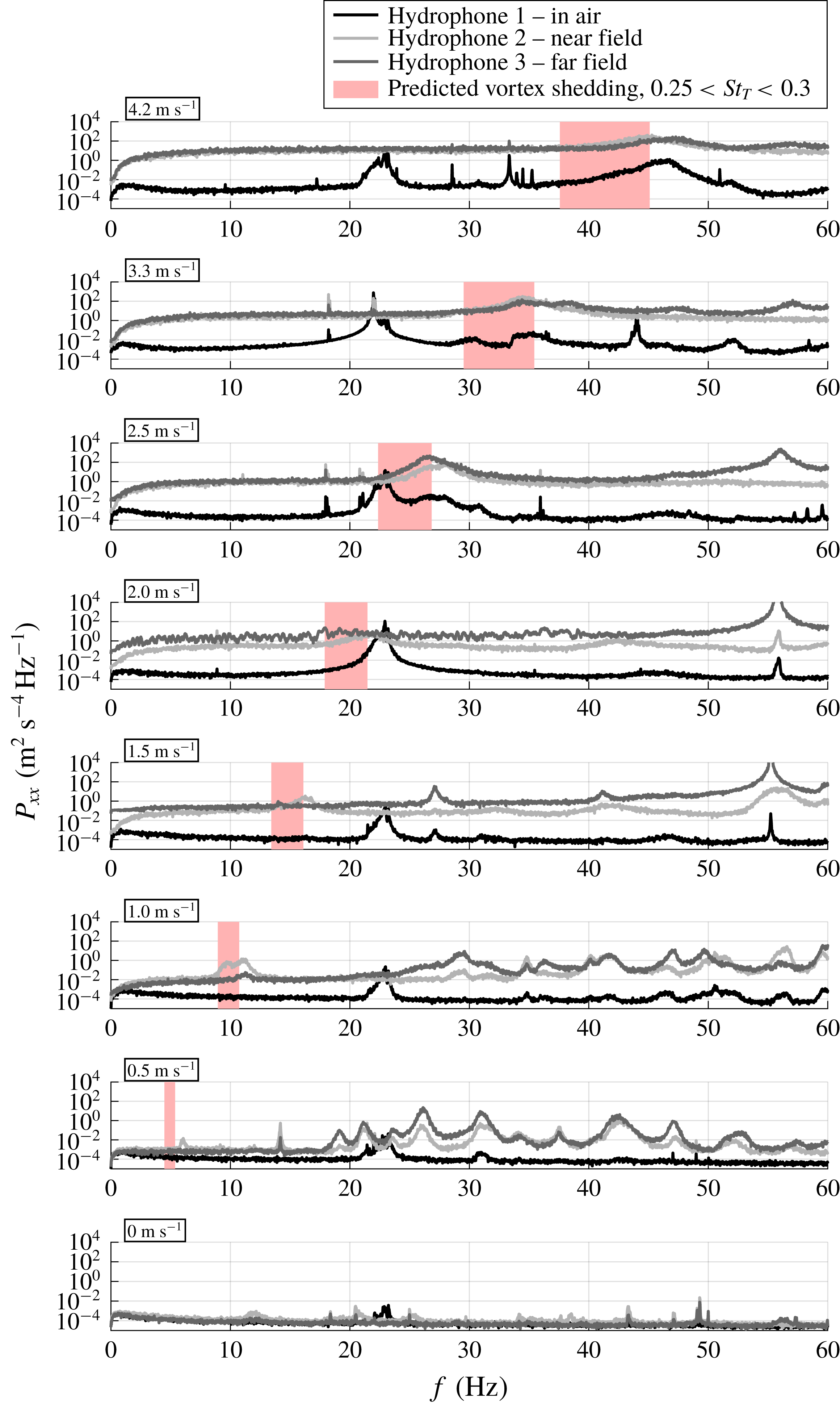
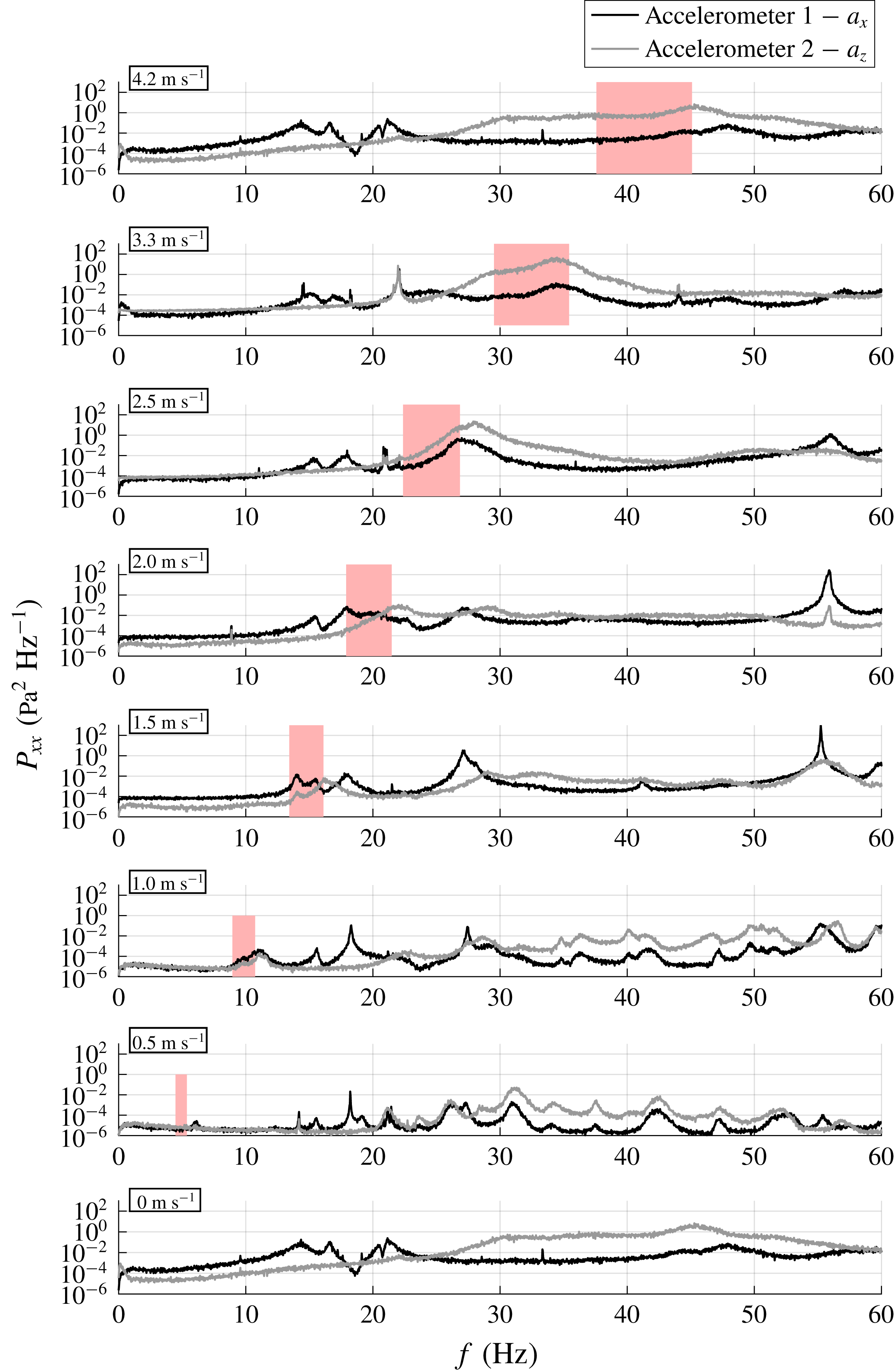
The focus is on the effect of flexibility of a lifting surface upon the hydrodynamic loads, the associated deflections and the scaling thereof. We will also show results demonstrating an amplified structural response when the vortex-shedding frequency coincides with one of the foil natural frequencies in water, i.e. lock-in condition. Finally, we will show the flow-induced vibration of a hydrofoil in cavitating conditions, which excited a broad frequency band – including the hydrofoil natural frequencies – but did not produce resonance because spanwise variations in the cavity pattern caused the cavity shedding to become incoherent.
1.2 Overview
Previous work published by the authors (Harwood, Young & Ceccio Reference Harwood, Young and Ceccio2016b ) has addressed the purely hydrodynamic aspects of ventilated flows by describing the flow regimes and ventilation transition mechanisms occurring on rigid surface-piercing hydrofoils. The present work builds upon those experiments by additionally considering cavitation and hydrofoil flexibility. Reviews of multi-phase flow and FSI are presented in §§ 2 and 3. The experimental approach (much of which is shared with Part 2 of this paper) is described in § 4. The steady-state hydrodynamic and hydroelastic responses are covered in § 5, which includes the two-dimensional/two-degree-of-freedom (2D-2DOF) model in § 5.1, the hydrodynamic loads in §§ 5.2 and 5.3 and the flow-induced hydroelastic coupling in § 5.4. Unsteady flow-induced vibration is described in § 6.
2 Multi-phase flows on surface-piercing bodies
The study of atmospheric ventilation on lifting devices dates to the mid-20th century (Acosta Reference Acosta1973), when surface-piercing hydrofoils were widely used as a means of passive lift control on fast hydrofoil-supported vessels – most often ferries and patrol craft. In addition to surface-piercing hydrofoils, ventilation affects surface-piercing struts and propellers, shallowly immersed hydrofoils and thrusters and a variety of fully submerged bodies with forced air-injection systems, which utilize ventilated cavities as means of reducing skin-friction drag and avoiding cavity-induced noise and erosion at high speeds. Vaporous cavitation has enjoyed a similarly long period of research and application. Efforts have focused in particular upon the mitigation of unwanted cavitation at high speeds. Alternatively, supercavitating propellers, hydrofoils and torpedoes are designed to encourage the development of extensive cavitating regions (supercavitation) to reduce skin-friction drag and minimize erosion and noise from partial or cloud cavities – applications overlapping with that of forced ventilation.
With the wealth of literature that exists in multi-phase flows, the terminology has become difficult to navigate without ambiguity. For example, the terms ‘natural cavity’, ‘vaporous cavity’ or simply ‘cavity’, are all used to describe the vaporization of liquid into its gaseous phase, making them distinct from ‘artificial cavity’, ‘ventilated cavity’, ‘natural ventilation’, ‘aeration’ or simply ‘ventilation’. To pre-empt a confusion of the various terminology, the language used in the recent review by Young et al. (Reference Young, Harwood, Miguel, Ward and Ceccio2017) will be adopted, which is briefly summarized below.
Natural ventilation, or simply ventilation, describes the case when a cavity is filled with air entrained from a nearby free surface (Acosta Reference Acosta1973; Faltinsen Reference Faltinsen2005). Naturally ventilated cavities are so named because they can persist under the supply of gas naturally entrained from the atmosphere. As a result, the pressure inside of the cavity is everywhere atmospheric, notwithstanding small dynamic pressure variations due to gas velocities inside of the cavity.
Vaporous cavitation, or simply cavitation, refers to the phase change of the working fluid from liquid to vapour. Cavitation typically occurs when the local absolute pressure decreases to near the saturated vapour pressure of the liquid. This criterion is complicated by additional factors such as surface finish, water quality (dissolved gas content or nucleation concentration) and viscous effects, all of which modify inception of vaporous cavities (Franc et al. Reference Franc, Franc, Michel and Michel2004; Morch Reference Morch2009; Brennen Reference Brennen2013; De Graaf, Pearce & Brandner Reference De Graaf, Pearce and Brandner2016).
Ventilation shares numerous similarities with vaporous cavitation. Both can lead to topologically similar flows, and cavities in both cases scale with the cavitation number defined based on the cavity pressure (more details in § 2.1). The physics underpinning the two multi-phase flows are quite different, however. Cavitation involves bi-directional transitions between the liquid and vapour phases through vaporization and condensation. Ventilation, on the other hand, involves only the transport of non-condensable gas around the submerged portion of a body as the primary mechanism of gas ingress and egress, and does not involve significant phase change. As a result, the dynamics of unsteady ventilated and vaporous cavities can be very different.
2.1 Parameters governing multi-phase flow on surface-piercing bodies
A consensus among ventilation researchers (Breslin & Skalak Reference Breslin and Skalak1959; Waid Reference Waid1968; Rothblum, Mayer & Wilburn Reference Rothblum, Mayer and Wilburn1969; Swales et al. Reference Swales, Wright, Mcgregor and Rothblum1974; Rothblum Reference Rothblum1977; Harwood Reference Harwood2016; Harwood et al. Reference Harwood, Young and Ceccio2016b ) holds that natural ventilation on a strut or hydrofoil occurs only when local wetted pressures are lower than the ambient pressure at the free surface, at least some flow separation is present on the lifting surface and there is a continuously available path of ingress for air to replenish an incipient or fully developed ventilated cavity.
The same body of literature indicates that the character of ventilated flow depends upon the depth-based Froude number (
 $Fn_{h}$
), the immersed aspect ratio (
 $AR_{h}$
) and the attack angle (
 $\unicode[STIX]{x1D6FC}$
). The former two are defined as,
 $$\begin{eqnarray}\displaystyle & \displaystyle Fn_{h}=\frac{U}{\sqrt{gh}}, & \displaystyle\end{eqnarray}$$
 $$\begin{eqnarray}\displaystyle & \displaystyle AR_{h}=\frac{h}{c}. & \displaystyle\end{eqnarray}$$
Here,
 $h$
is the depth of the hydrofoil’s free tip beneath the plane of the undisturbed free surface and
 $c$
is the foil’s chord length. The generalized cavitation number is defined in a plane at a depth
 $z$
beneath the free surface as,
 $$\begin{eqnarray}\unicode[STIX]{x1D70E}_{c}(z)=\frac{P_{\infty }(z)-P_{c}}{\unicode[STIX]{x1D70C}_{f}U^{2}/2},\end{eqnarray}$$
where
 $P_{\infty }=P_{0}+\unicode[STIX]{x1D70C}_{f}gz$
is the free-stream pressure at the depth (
 $z$
) being considered,
 $P_{0}$
is the absolute ambient pressure at the free surface,
 $P_{c}$
is the pressure inside the cavity and
 $\unicode[STIX]{x1D70C}_{f}$
is the fluid density. In naturally ventilated flows,
 $P_{c}=P_{0}$
and, as a consequence,
 $$\begin{eqnarray}\unicode[STIX]{x1D70E}_{c}(z)=\frac{2}{Fn_{h}^{2}}\frac{z}{h}.\end{eqnarray}$$
To assign a unique value to
 $\unicode[STIX]{x1D70E}_{c}$
, the convention will be adopted in § 5.3 to define
 $\unicode[STIX]{x1D70E}_{c}$
at the middle of the submerged span (
 $z=h/2$
).
If vaporous cavitation is being considered,
 $P_{c}=P_{v}$
(the saturated vapour pressure of the working liquid), and the vaporous cavitation number is defined as,
 $$\begin{eqnarray}\unicode[STIX]{x1D70E}_{v}=\frac{P_{0}-P_{V}}{\unicode[STIX]{x1D70C}_{f}U^{2}/2}.\end{eqnarray}$$
Thus,
 $\unicode[STIX]{x1D70E}_{v}$
is a special case of
 $\unicode[STIX]{x1D70E}_{c}$
, defined at the free surface for vapour-filled cavities. Under special circumstances, it is possible to support separate vaporous and ventilated cavities on the same lifting surface (Waid Reference Waid1968; Rothblum et al.
Reference Rothblum, Mayer and Wilburn1969; Olofsson Reference Olofsson1996; Young & Brizzolara Reference Young and Brizzolara2013; Harwood Reference Harwood2016), in which case the dissimilar cavities are separated by a thin layer of liquid water. In cases where vaporous cavities ingest a limited quantity of air, the cavity will be of a homogeneous, but mixed, composition (Young & Brizzolara Reference Young and Brizzolara2013; Young et al.
Reference Young, Harwood, Miguel, Ward and Ceccio2017).
2.1.1 Flow regimes on a surface-piercing hydrofoil
When a ventilated or vaporous cavity develops on a nominally two-dimensional (2-D) hydrofoil section, the observed length of the cavity (
 $L_{c}$
), relative to the chord length (
 $c$
) of the hydrofoil section, is used to classify the flow as fully wetted (
 $L_{c}=0$
), partially cavitating (
 $0<L_{c}<c$
), or supercavitating (
 $L_{c}\geqslant c$
) flow. Rothblum et al. (Reference Rothblum, Mayer and Wilburn1969), Rothblum (Reference Rothblum1977), Harwood (Reference Harwood2016), Harwood et al. (Reference Harwood, Young and Ceccio2016b
) and Young et al. (Reference Young, Harwood, Miguel, Ward and Ceccio2017) showed that three-dimensional (3-D) flow over a hydrofoil defies such a simple distinction. This was shown to be especially true at low and moderate values of
 $Fn_{h}$
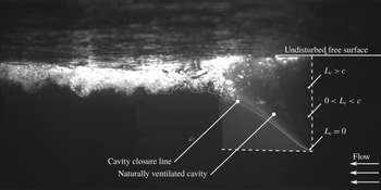
, where the hydrostatic pressure gradient is appreciably large relative to the chordwise pressure gradients on the hydrofoil. Consider figure 1, which depicts natural ventilation of the aluminium hydrofoil described by Harwood et al. (Reference Harwood, Young and Ceccio2016b
). Sectional cuts taken through the three spanwise locations called out in the figure are classified as fully wetted, partially cavitating and supercavitating, making its classification ambiguous. Harwood et al. (Reference Harwood, Young and Ceccio2016b
), and later Young et al. (Reference Young, Harwood, Miguel, Ward and Ceccio2017), recommended a standardization of the vernacular used to discuss such flows – a convention adopted in this work and extended to include flows with vaporous cavitation. Four flow regimes are thus defined: fully wetted (FW) flow, partially ventilated (PV) flow, partially cavitating (PC) flow and fully ventilated (FV) flow, depicted respectively in figures 2, 3, 4 and 5. These regimes are briefly reviewed below. Note that all of the photographic images in this section depict the experiments described in § 4.
Example of a naturally ventilated cavity flow at
 $\unicode[STIX]{x1D6FC}=15^{\circ }$
,
 $Fn_{h}=1.25$
,
 $AR_{h}=1.0$
. At different points along the span, the individual sections are fully wetted, partially cavitating and supercavitating, making the flow regime of the 3-D cavity ambiguous.

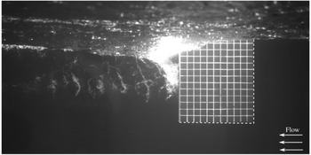
Fully wetted flow is defined as the flow regime where no pronounced air entrainment occurs over the suction or pressure surfaces of the hydrofoil. On lifting surfaces possessing a blunt trailing edge (including the geometry considered in this work), FW flow includes the base-cavitating or base-ventilating flows that occur, respectively, when gas is entrained in the separated wake of the trailing edge or when shear layer cavitation develops at the boundaries of the wake. Figure 2 depicts the suction surface of a surface-piercing hydrofoil in fully wetted conditions, with a ventilated base cavity that extends approximately half-way from the free surface to the immersed tip.
Photo of FW flow over the suction side of a flexible surface-piercing hydrofoil at CNR INM (described in § 4). Run conditions:
 $\unicode[STIX]{x1D6FC}=5^{\circ }$
;
 $Fn_{h}=2$
;
 $AR_{h}=1$
;
 $P_{0}=1~\text{bar}$
;
 $\unicode[STIX]{x1D70E}_{v}=18$
.

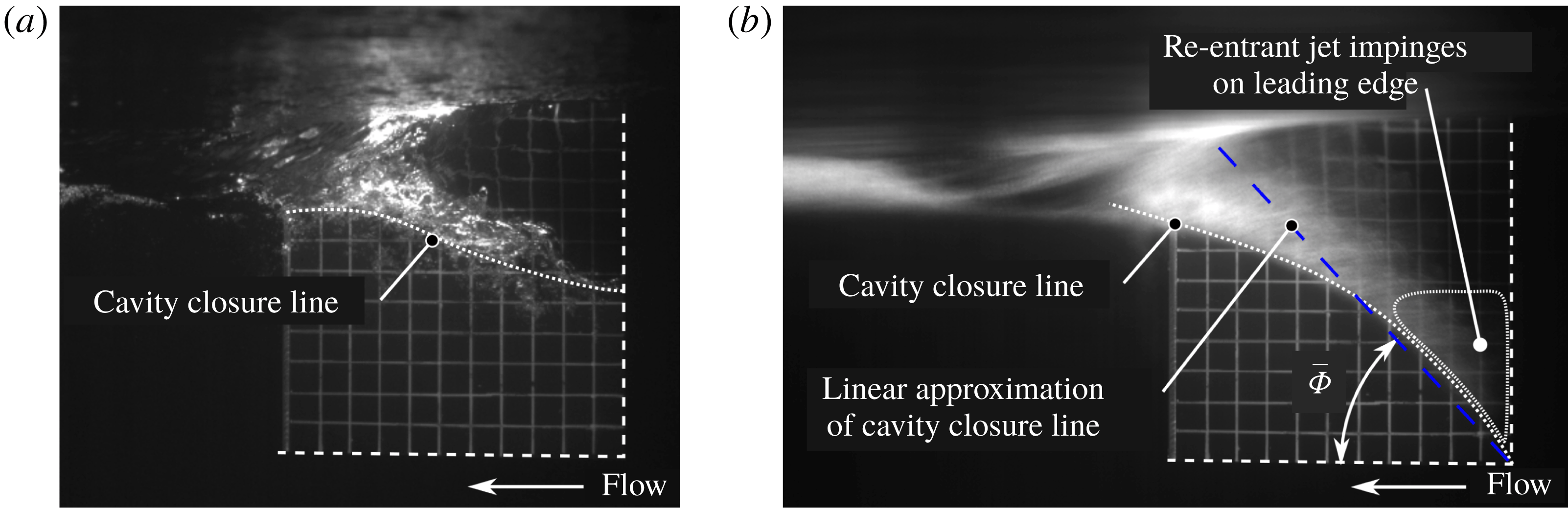
Photos of PV flow over the suction surface of a flexible surface-piercing hydrofoil at CNR INM (described in § 4). (a) Shows a cavity that does not reach the immersed tip. Run conditions:
 $\unicode[STIX]{x1D6FC}=15^{\circ };Fn_{h}=1;AR_{h}=1;P_{0}=1~\text{bar}$
. (b) Shows a cavity with a closure angle exceeding the
 $45^{\circ }$
condition proposed by Harwood et al. (Reference Harwood, Young and Ceccio2016b
), resulting in a re-entrant jet that impinges on the leading edge of the cavity. Run conditions:
 $\unicode[STIX]{x1D6FC}=12^{\circ };Fn_{h}=1.2;AR_{h}=1;P_{0}=47~\text{mbar}$
.

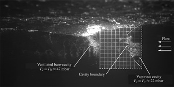
Photo of PC flow over the suction surface of a flexible surface-piercing hydrofoil at CNR INM (described in § 4). Run conditions:
 $\unicode[STIX]{x1D6FC}=5^{\circ }$
;
 $Fn_{h}=2.17$
;
 $AR_{h}=1$
;
 $P_{0}=47~\text{mbar}$
;
 $\unicode[STIX]{x1D70E}_{v}=0.35$
. In addition to the vaporous cavity near the leading edge, naturally ventilated flow is visible downstream from the blunt trailing edge.

Photo of FV flow over the suction surface of a flexible surface-piercing hydrofoil at CNR INM (described in § 4). Run conditions:
 $\unicode[STIX]{x1D6FC}=15^{\circ };Fn_{h}=2;AR_{h}=1;P_{0}=1~\text{bar}$
.

Partially ventilated flow is defined as the entrainment of non-condensable gas (e.g. air) over a limited portion of the suction surface of a hydrofoil. PV flow occurs when the gaseous cavity either (i) does not extend along the entire immersed span of the hydrofoil, or (ii) is shorter than the chord length, with a closure line occurring at an angle
 $\bar{\unicode[STIX]{x1D6F7}}>45^{\circ }$
, measured from the streamwise direction (Harwood et al.
Reference Harwood, Young and Ceccio2016b
). Note that the latter criterion is based on the kinematics of the re-entrant jet, and not on a requirement that at least 50 % of the hydrofoil surface be enveloped in a cavity. Flow around the cavity closure is reflected by the constant-pressure boundary of the cavity (de Lange & de Bruin Reference de Lange and de Bruin1997), so when
 $\bar{\unicode[STIX]{x1D6F7}}>45^{\circ }$
, the resulting re-entrant flow destabilizes the cavity. A classic example of such an instability is cyclic sheet-cloud cavitation (Kawakami et al.
Reference Kawakami, Fuji, Tsujimoto and Arndt2008; Young et al.
Reference Young, Harwood, Miguel, Ward and Ceccio2017). This criterion is thus insensitive to the immersion of the hydrofoil, but requires modification if it is to be applied to swept foils. Figure 3(a) depicts an example of the former (case a). Figure 3(b) depicts the latter (case b), which causes the re-entrant jet to move upstream and undercut the attached cavity (Harwood et al.
Reference Harwood, Young and Ceccio2016b
).
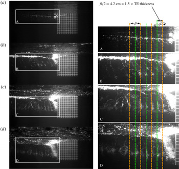
Partially cavitating flow occurs when the cavity is filled with the vaporous form of the working fluid – water in the flows discussed in this work. An example of PC flow is shown in figure 4, which was recorded while running a free-surface water channel under reduced pressure (described further in § 4). The vaporous cavity forms near the leading edge (LE) and exhibits a nearly elliptical distribution of cavity lengths (a result of the finite aspect ratio and zero loading condition at the free surface and the free tip). Note that the vaporous cavity below the free surface is separated from the non-condensable gas above only by a thin layer of liquid water, dubbed the free-surface ‘seal’ (Rothblum et al. Reference Rothblum, Mayer and Wilburn1969; Swales et al. Reference Swales, Wright, Mcgregor and Rothblum1974). The seal is formed where the pressure on the hydrofoil is made constant by the proximity of the free surface. The limited cavity length leads to a 3-D re-entrant jet and attendant cavity shedding. Unlike a 2-D re-entrant jet, where the cavity shedding occurs with a constant chord-based Strouhal number (Franc et al. Reference Franc, Franc, Michel and Michel2004; Brennen Reference Brennen2013; Young et al. Reference Young, Harwood, Miguel, Ward and Ceccio2017), the 3-D cavity in figure 4 creates a non-uniform re-entrant jet; the cavity shedding may lack coherent structure or well-defined periodicity as a result.
Fully ventilated flow requires a ventilated cavity to extend along the entire immersed span and either (i) exceed the chord length everywhere or (ii) close along an angle
 $\hat{\unicode[STIX]{x1D6F7}}\leqslant 45^{\circ }$
(Harwood et al.
Reference Harwood, Young and Ceccio2016b
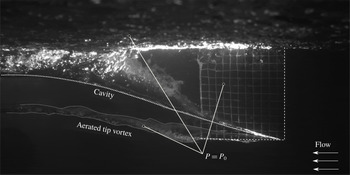
). FV flow may thus follow from the stabilization of a PV flow, or may follow a perturbation to a FW flow. Satisfaction of the prior conditions ensures that, if a re-entrant jet is present, its streamwise velocity component carries it downstream where it does not compromise the stability of an attached cavity. Figure 5 depicts an FV flow in which both conditions are obviously satisfied, leading to a large, smooth-walled cavity that envelops the near (suction) surface and feeds atmospheric gas to a large aerated tip vortex.
The transition between the various flow regimes have been further explored by Breslin & Skalak (Reference Breslin and Skalak1959), Waid (Reference Waid1968), Swales et al. (Reference Swales, Wright, Mcgregor and Rothblum1974) and Harwood et al. (Reference Harwood, Young and Ceccio2016b ). Ventilation formation was described as the collection of processes that increase the size or stability of a ventilated cavity, including inception and stabilization. Ventilation elimination encompasses those mechanisms that detract from the size or stability of a cavity, including washout and re-wetting. Young et al. (Reference Young, Harwood, Miguel, Ward and Ceccio2017) summarized a taxonomy of the mechanisms by which the flow around a surface-piercing hydrofoil (the same hydrofoil used in this work) transitions between regimes.
3 Hydroelasticity of lifting surfaces
Highly loaded appendages of moderate-to-high aspect ratios, such as propeller blades, rudders, hydrofoils and control surfaces are particularly likely to deform under operational loads – especially with increasing use of non-metallic construction materials that include composites and polymers with low material moduli. It is thus prudent to consider the static and dynamic FSI of flexible lifting surfaces under a variety of loading conditions and in a variety of flow regimes (Liu & Young Reference Liu and Young2009, Reference Liu and Young2010; Young et al. Reference Young, Motley, Barber, Chae and Garg2016, Reference Young, Garg, Brandner, Pearce, Butler, Clarke and Phillips2018a ,Reference Young, Garg, Brandner, Pearce, Butler, Clarke and Phillips b ).
FSI responses are broadly classified according to the relative mass ratio,
 $$\begin{eqnarray}\unicode[STIX]{x1D707}=\sqrt{\frac{4m}{\unicode[STIX]{x1D70C}_{f}\unicode[STIX]{x03C0}c^{2}}},\end{eqnarray}$$
which may be interpreted as the ratio of the solid mass of a foil section (
 $m$
) to the fluid mass contained inside of its circumscribed circle, both defined per unit length. Hydroelasticity is the sub-discipline of FSI dealing with flexible bodies in dense fluids (
 $\unicode[STIX]{x1D707}\lesssim 2$
). This distinguishes it from the more-mature field of aeroelasticity, wherein flexible structures interact with light gases (
 $\unicode[STIX]{x1D707}\gtrsim 4$
) (Bisplinghoff, Ashley & Halfman Reference Bisplinghoff, Ashley and Halfman2013; Chae, Akcabay & Young Reference Chae, Akcabay and Young2013; Chae et al.
Reference Chae, Akcabay, Lelong, Astolfi and Young2016). Operation in water poses a number of unique challenges not present in aeroelasticity. As implied by the value of
 $\unicode[STIX]{x1D707}$
, the density of the fluid tends to be much greater relative to that of the solid, increasing the importance of fluid inertia, fluid damping and fluid disturbing forces. Numerical work by Fu & Price (Reference Fu and Price1987), Chae et al. (Reference Chae, Akcabay and Young2013, Reference Chae, Akcabay, Lelong, Astolfi and Young2016), Akcabay & Young (Reference Akcabay and Young2014) and Akcabay et al. (Reference Akcabay, Chae, Young, Ducoin and Astolfi2014a
,Reference Akcabay, Young, Lelong and Astolfi
b
), experimental work by Besch & Liu (Reference Besch and Liu1971, Reference Besch and Liu1973, Reference Besch and Liu1974), Blake (Reference Blake1972), Blake & Maga (Reference Blake and Maga1975), Fu & Price (Reference Fu and Price1987), Akcabay et al. (Reference Akcabay, Chae, Young, Ducoin and Astolfi2014a
), Chae et al. (Reference Chae, Akcabay, Lelong, Astolfi and Young2016), Harwood et al. (Reference Harwood, Stankovich, Young and Ceccio2016a
) and a recent review by Young et al. (Reference Young, Motley, Barber, Chae and Garg2016) have demonstrated that fluid inertia, damping and disturbing forces can dominate the governing equations of motion when relative mass ratios are small. Speeds also tend to be smaller by one to two orders of magnitude in water than in air, resulting in lower Reynolds numbers and increased viscous effects. Additionally, many marine applications involve multiple fluids, in the form of a free-surface and multi-phase flows. In some cases, particularly in steady flow, where inertial and damping effects are small, aeroelastic theories are adequate for hydroelastic analyses. However, as flows become more dynamic, and as inertial, viscous and other nonlinear forces become increasingly dominant, sufficiently accurate treatment will require modified theory, time-domain simulation and/or new empirical descriptions.
For the purposes of this study, deformable structures will be assumed to be linearly elastic. Such a structure, placed in a fluid may be represented by the matrix equations of motion,
 $$\begin{eqnarray}\unicode[STIX]{x1D648}_{\boldsymbol{s}}\ddot{\boldsymbol{X}}+(\unicode[STIX]{x1D63E}_{\boldsymbol{s}}+\unicode[STIX]{x1D642}_{\boldsymbol{s}}\unicode[STIX]{x1D64E}^{D})\dot{\boldsymbol{X}}+\unicode[STIX]{x1D646}_{\boldsymbol{ s}}\boldsymbol{X}=\boldsymbol{F}_{\boldsymbol{E}\boldsymbol{X}}+\boldsymbol{F}_{\boldsymbol{f}\boldsymbol{l}},\end{eqnarray}$$
where
 $\unicode[STIX]{x1D648}_{\boldsymbol{s}}$
,
 $\unicode[STIX]{x1D63E}_{\boldsymbol{s}}$
,
 $\unicode[STIX]{x1D642}_{\boldsymbol{s}}$
and
 $\unicode[STIX]{x1D646}_{\boldsymbol{s}}$
are respectively the solid mass, viscous and hysteretic structural damping and stiffness matrices;
 $\unicode[STIX]{x1D64E}^{D}$
is a scale matrix, defined as
 $$\begin{eqnarray}\unicode[STIX]{x1D61A}_{ij}=\unicode[STIX]{x1D6FF}_{ij}\frac{|X_{i}|}{|\dot{X_{j}}|},\end{eqnarray}$$
where
 $\unicode[STIX]{x1D6FF}$
is the Kronecker delta, such that the hysteretic damping force acts proportionally to the displacement, but in phase with the velocity. The vector of nodal displacements
 $\boldsymbol{X}$
represents some finite number of degrees of freedom,
 $\boldsymbol{F}_{\boldsymbol{E}\boldsymbol{X}}$
is a vector of external perturbations and
 $\boldsymbol{F}_{\boldsymbol{f}\boldsymbol{l}}$
is the hydrodynamic force vector, which includes all steady and unsteady fluid loads. The ‘passive’ hydroelastic interactions in this work concern cases in which
 $\boldsymbol{F}_{\boldsymbol{E}\boldsymbol{X}}=\mathbf{0}$
. Part 2 of this paper addresses active hydroelasticity (
 $\boldsymbol{F}_{\boldsymbol{E}\boldsymbol{X}}\neq \mathbf{0}$
).
The fluid load vector
 $\boldsymbol{F}_{\boldsymbol{f}\boldsymbol{l}}$
may be further decomposed to yield,
 $$\begin{eqnarray}\boldsymbol{F}_{\boldsymbol{f}\boldsymbol{l}}=\boldsymbol{F}_{\boldsymbol{s}\boldsymbol{f},\boldsymbol{r}}+\boldsymbol{F}_{\boldsymbol{u}\boldsymbol{f},\boldsymbol{r}}-(\unicode[STIX]{x1D648}_{\boldsymbol{f}}\ddot{\boldsymbol{X}}+\unicode[STIX]{x1D63E}_{\boldsymbol{f}}\dot{\boldsymbol{X}}+\unicode[STIX]{x1D646}_{\boldsymbol{f}}\boldsymbol{X}).\end{eqnarray}$$
The fluid mass
 $\unicode[STIX]{x1D648}_{\boldsymbol{f}}$
, fluid damping
 $\unicode[STIX]{x1D63E}_{\boldsymbol{f}}$
and fluid hydrodynamic stiffness
 $\unicode[STIX]{x1D646}_{\boldsymbol{f}}$
account for the fluid forces respectively in phase with the acceleration, velocity and displacements of the flexible structure. Note that ‘fluid stiffness’ is a somewhat contentious term; the product
 $(\unicode[STIX]{x1D646}_{\boldsymbol{f}}\boldsymbol{X})$
is sometimes dubbed the fluid disturbing, de-stiffening or restoring force instead. In this work, the term ‘hydrodynamic stiffness’ is adopted, in recognition of the fact that
 $\unicode[STIX]{x1D646}_{\boldsymbol{f}}$
is non-zero only in moving fluids.
 $\boldsymbol{F}_{\boldsymbol{s}\boldsymbol{f},\boldsymbol{r}}$
is the steady fluid load on an equivalent rigid lifting geometry at the same (undeformed) attitude as the flexible structure;
 $\boldsymbol{F}_{\boldsymbol{u}\boldsymbol{f},\boldsymbol{r}}$
encompasses the various unsteady fluid forces acting on the equivalent rigid body (e.g. nonlinear forces, cavity shedding or vortex shedding). Note that even when the lifting surface under consideration is in an undeformed state
 $(\boldsymbol{X}=0)$
, there may be a non-zero fluid load, e.g. that due to a non-zero angle of attack or camber of a lifting surface. The steady fluid force takes the form of a bias,
 $$\begin{eqnarray}\boldsymbol{F}_{\boldsymbol{s}\boldsymbol{f},\boldsymbol{r}}=-\unicode[STIX]{x1D646}_{\boldsymbol{f}}\boldsymbol{X}_{\mathbf{0}},\end{eqnarray}$$
where
 $\boldsymbol{X}_{\mathbf{0}}$
is measured from the displacement vector yielding zero fluid load.
After regrouping terms, the equations of motion become,
 $$\begin{eqnarray}\displaystyle & & \displaystyle (\unicode[STIX]{x1D648}_{\boldsymbol{s}}+\unicode[STIX]{x1D648}_{\boldsymbol{f}})\ddot{\boldsymbol{X}}+(\unicode[STIX]{x1D63E}_{\boldsymbol{s}}+\unicode[STIX]{x1D63E}_{\boldsymbol{f}})\dot{\boldsymbol{X}}+\unicode[STIX]{x1D642}_{\boldsymbol{s}}\unicode[STIX]{x1D64E}^{D}\dot{\boldsymbol{X}}+(\unicode[STIX]{x1D646}_{\boldsymbol{s}}+\unicode[STIX]{x1D646}_{\boldsymbol{f}})\boldsymbol{X}\cdots \nonumber\\ \displaystyle & & \displaystyle \quad =\boldsymbol{F}_{\boldsymbol{E}\boldsymbol{X}}+\boldsymbol{F}_{\boldsymbol{s}\boldsymbol{f},\boldsymbol{r}}+\boldsymbol{F}_{\boldsymbol{u}\boldsymbol{f},\boldsymbol{r}}.\end{eqnarray}$$
Consolidating the preceding terms into the effective system mass, damping and stiffness matrices,
 $$\begin{eqnarray}\left.\begin{array}{@{}c@{}}\unicode[STIX]{x1D648}=\unicode[STIX]{x1D648}_{\boldsymbol{s}}+\unicode[STIX]{x1D648}_{\boldsymbol{f}},\\ \hspace{0.0pt}\unicode[STIX]{x1D63E}=\unicode[STIX]{x1D63E}_{\boldsymbol{s}}+\unicode[STIX]{x1D63E}_{\boldsymbol{f}},\\ \hspace{0.0pt}\unicode[STIX]{x1D646}=\unicode[STIX]{x1D646}_{\boldsymbol{s}}+\unicode[STIX]{x1D646}_{\boldsymbol{f}},\end{array}\right\}\end{eqnarray}$$
results in the general equations of motion for a hydroelastic system, e.g. the flexible hydrofoil upon which the present work is focused,
 $$\begin{eqnarray}\unicode[STIX]{x1D648}\ddot{\boldsymbol{X}}+(\unicode[STIX]{x1D63E}+\unicode[STIX]{x1D642}_{\boldsymbol{s}}\unicode[STIX]{x1D64E}^{D})\dot{\boldsymbol{X}}+\unicode[STIX]{x1D646}\boldsymbol{X}=\boldsymbol{F}_{\boldsymbol{ E}\boldsymbol{X}}+\boldsymbol{F}_{\boldsymbol{s}\boldsymbol{f},\boldsymbol{r}}+\boldsymbol{F}_{\boldsymbol{u}\boldsymbol{f},\boldsymbol{r}}.\end{eqnarray}$$
3.1 Steady hydroelasticity
Steady hydroelasticity describes the equilibrium condition of (3.8) in the absence of first and second derivatives and when
 $\boldsymbol{F}_{\boldsymbol{u}\boldsymbol{f},\boldsymbol{r}}=0$
. In these cases, the linear response is,
 $$\begin{eqnarray}\boldsymbol{X}=(\unicode[STIX]{x1D646}_{\boldsymbol{s}}+\unicode[STIX]{x1D646}_{\boldsymbol{f}})^{-1}(\boldsymbol{F}_{\boldsymbol{ E}\boldsymbol{X}}+\boldsymbol{F}_{\boldsymbol{s}\boldsymbol{f},\boldsymbol{r}}).\end{eqnarray}$$
Static divergence occurs when the hydrodynamic stiffness negates the structural stiffness of the system, such that the effective stiffness
 $\unicode[STIX]{x1D646}$
becomes singular and no resulting equilibrium response exists to a steady, non-zero
 $\boldsymbol{F}_{\boldsymbol{s}\boldsymbol{f},\boldsymbol{r}}$
or
 $\boldsymbol{F}_{\boldsymbol{E}\boldsymbol{X}}$
. For most common lifting geometries, where the elastic axes do not coincide with the centres of pressure,
 $\unicode[STIX]{x1D646}_{\boldsymbol{f}}$
contains off-diagonal elements termed ‘flow-induced’, or hydrodynamic, bend-twist coupling. A series of recent experiments have explored the effects of hydrofoil flexibility and material anisotropy on FSI. Zarruk et al. (Reference Zarruk, Brandner, Pearce and Phillips2014) used a series of unswept, tapered hydrofoil with a modified NACA 0009 section manufactured from metallic and composite materials with two different fibre orientation angles to study the steady FSI response of hydrofoils in a cantilevered configuration. They found that the fibre orientation affected both the steady-state loads and lift distributions in the cases of the composite foils. Recent experiments published by Young et al. (Reference Young, Garg, Brandner, Pearce, Butler, Clarke and Phillips2018a
) used the same geometries, with an additional fibre orientation angle to affect material bend-twist coupling. A 2D-2DOF model was used with assumed modes to scale the static FSI response of composite hydrofoils in subcavitating flow. As mentioned previously, the work showed that when the centre of pressure was separated from the elastic axis, a bend-twist coupling was induced by the flow that could be enhanced or retarded by the choice of ply bias in the composite layup. Recent experiments and reduced-order models published by Chae, Akcabay & Young (Reference Chae, Akcabay and Young2017) and Young et al. (Reference Young, Garg, Brandner, Pearce, Butler, Clarke and Phillips2018a
) similarly demonstrated through simulations that material anisotropy could be used to counteract the flow-induced bend-twist coupling, as well as delay stall, static divergence and cavitation inception.
3.2 Unsteady hydroelasticity
Forced motions, as the name implies, result from an external force represented by
 $\boldsymbol{F}_{\boldsymbol{E}\boldsymbol{X}}$
. A harmonic component of
 $\boldsymbol{F}_{\boldsymbol{E}\boldsymbol{X}}$
elicits a harmonic structural response at the same frequency. Resonance occurs when said frequency matches a natural frequency of the excited system (or some harmonic or subharmonic thereof, in the case of nonlinear systems), resulting in large-amplitude motions of the associated normal mode of that structure. External excitations include operational sources such as vibrations of engines, shafting or propellers, or direct perturbations of a structure, such as that provided by a shaker motor attached to a structure during vibration testing. When the excitation arises from the flow itself, the force is grouped into the fluid force vector
 $\boldsymbol{F}_{\boldsymbol{u}\boldsymbol{f},\boldsymbol{r}}$
and the resulting motion is referred to as flow-induced vibration. Periodic cavity shedding, vortex shedding and boundary-layer instability typify periodic flow-induced excitations (Ducoin, Astolfi & Gobert Reference Ducoin, Andre and Gobert2012; Chae et al.
Reference Chae, Akcabay and Young2013, Reference Chae, Akcabay, Lelong, Astolfi and Young2016, Reference Chae, Akcabay and Young2017; Akcabay et al.
Reference Akcabay, Chae, Young, Ducoin and Astolfi2014a
).
Flow-induced vibration leads to a subtle variation on resonance, known as ‘lock-in’, which is a topic of § 6. Lock-in occurs when the flow phenomena creating the force and the motions of the affected body are inherently linked. A hydrodynamic mode can occur at a fixed frequency when the associated body is either rigid or when that frequency is far removed from any in situ structural modal frequencies of the body. Lock-in is said to occur when the hydrodynamic and structural frequencies are sufficiently close to one another that one or both processes are altered, and the individual spectral peaks merge to form a single peak. That peak will not necessarily be co-located with the frequencies of either the structural or the fluid mode in isolation (Sarpkaya Reference Sarpkaya1995; Williamson & Govardhan Reference Williamson and Govardhan2004). During lock-in, the fluid damping associated with the excited mode drops precipitously, reaching in extreme cases a negative value, which leads to an amplification of small motions and fluctuating fluid loads. If the structural modal damping is not sufficiently large to ensure a positive net damping, destructive vibrations may ensue, with large fluctuations in the fluid loads and material stresses resulting. A well-known example is the phenomenon of vortex-induced vibrations of cylindrical bodies. When the frequency of oscillation of a cylindrical body and the frequency of vortex shedding into the von Kármán street approach one another, the motions of the body will – to some extent – drive the frequency at which vortices are shed, and the two phenomena will lock in to a flow-induced resonance condition. Ausoni et al. (Reference Ausoni, Farhat, Avellan, Escaler and Egusquiza2005, Reference Ausoni, Farhat, Escaler, Egusquiza and Avellan2007) demonstrated that von Kármán vortex shedding drove lock-in resonance on a cantilevered hydrofoil in wetted and cavitating conditions. The onset of cavitation was found to disrupt lock-in by increasing the vortex-shedding frequencies beyond the lock-in range. Other examples include the phenomenon of propeller ‘singing’ and the high-frequency resonance induced in propeller blades by laminar-to-turbulent transition (Ducoin et al. Reference Ducoin, Andre and Gobert2012). When the frequency of the hydrodynamic force is outside of a finite band surrounding each structural normal mode, a lock-off condition prevails, in which non-resonant flow-induced vibrations are observed.
Flutter occurs when the effective damping of at least one mode of vibration becomes zero or negative, with the mode in question dubbed the flutter mode. As a result, the flutter mode extracts energy from the flow and grows in amplitude until either nonlinearities arrest further growth or material failure occurs. Flutter in coupled degrees of freedom is accompanied by coalescence of two or more modal frequencies toward the ‘flutter frequency’. The instability occurs when the effective modal damping of at least one mode becomes negative. This leads to an unbounded transfer of energy from a highly damped mode into the negatively damped flutter mode.
Akcabay et al. (Reference Akcabay, Chae, Young, Ducoin and Astolfi2014a ) used a combined experimental and numerical approach to show that cavity shedding elicited flow-induced vibration of a flexible hydrofoil and that the modulation of the added mass, damping and stiffness matrices were captured well by coupling a 2-D computational fluid dynamics (CFD) simulation to a 2-DOF structural model, where the static bending and twisting shape factors of the experimental model were used as the assumed modes in an application of Ritz’ method in order to bridge the 2-D model and 3-D experiments. The effects of the flow on the specific fluid force components were not explicitly quantified, however. Chae et al. (Reference Chae, Akcabay, Lelong, Astolfi and Young2016) and Lelong, Guiffant & André Astolfi (Reference Lelong, Guiffant and André Astolfi2017) used a flexible, cantilevered hydrofoil to demonstrate lock-in between the first bending modal frequency and the vaporous cavity shedding frequency across a narrow band of vaporous cavitation numbers. The modulation of fluid parameters caused by the unsteady cavitation was also observed to broaden the peaks in measured spectra of the tip bending and twisting motions.
Pearce et al. (Reference Pearce, Brandner, Garg, Young, Phillips and Clarke2017) and Smith et al. (Reference Smith, Venning, Giosio, Brandner, Pearce and Young2019) showed that – for the hydrofoil geometry studied by Zarruk et al. (Reference Zarruk, Brandner, Pearce and Phillips2014) and Young et al. (Reference Young, Garg, Brandner, Pearce, Butler, Clarke and Phillips2018a
) – the material bend-twist coupling affected cavity dynamics when vaporous cavitation was present by modifying the lock-in conditions for moderate values of
 $\unicode[STIX]{x1D70E}_{v}$
. For small values of
 $\unicode[STIX]{x1D70E}_{v}$
, the cavity shedding dynamics was found to overshadow the structural effects. It was shown by Young et al. (Reference Young, Garg, Brandner, Pearce, Butler, Clarke and Phillips2018b
) that material bend-twist coupling of the composite hydrofoils affected the maximum cavity length and shedding frequencies of Type II cavities (re-entrant jet driven). Type I shedding (shock-wave driven, as described by Ganesh, Makiharju & Ceccio (Reference Ganesh, Makiharju and Ceccio2016)) was also indirectly influenced by the composite layup angle, through the effect of material bend-twist coupling on maximum cavity lengths.
4 Experimental methodology
The experimental set-up used for this work is an expansion upon on the set-up used by Harwood et al. (Reference Harwood, Young and Ceccio2016b ). Tests were executed in two facilities. One rigid aluminium hydrofoil and two variants of a flexible polyvinyl chloride (PVC) hydrofoil were used. The aluminium hydrofoil is herein referred to as ‘Model 0’. The PVC hydrofoil and the reinforced PVC hydrofoil are respectively dubbed ‘Model 1’ and ‘Model 2’.
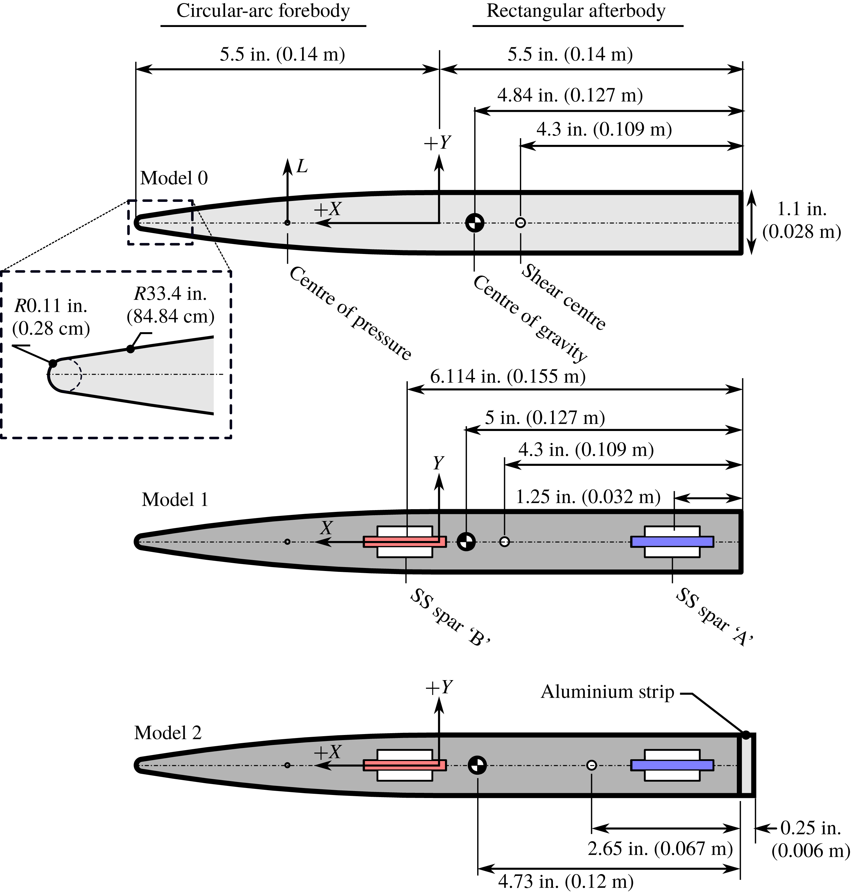
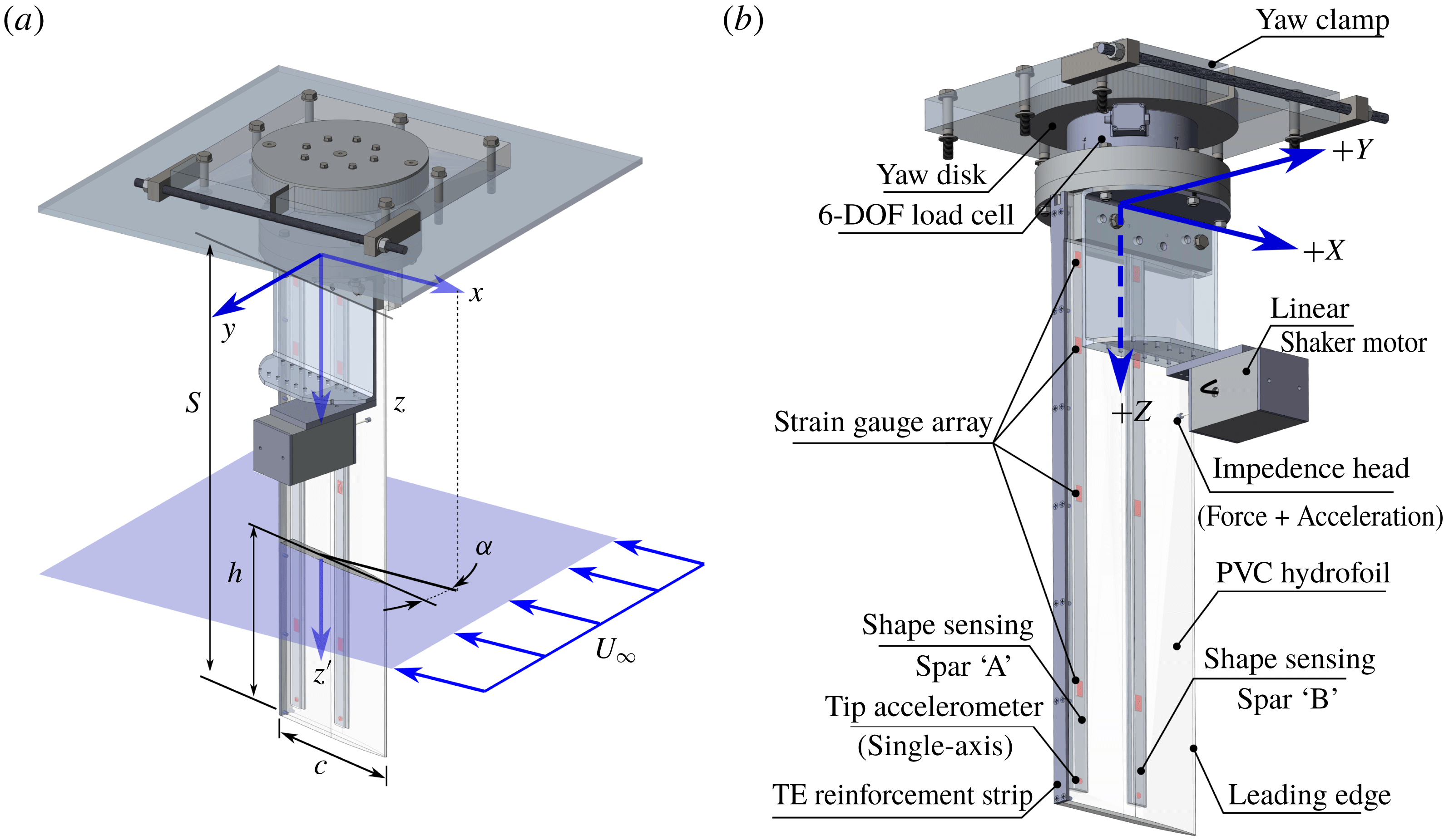
All models had semi-ogive section shapes and rectangular plan forms with a common span of 91.4 cm (36 inches) and chord lengths of 27.9 or 28.58 cm (11 or 11.25 inches). In all cases, the section was constant along the span. Figure 6 shows a comparison of the sections of Model 0, Model 1 and Model 2, with the locations of the mass centres and shear centres indicated.
Cross-sections of aluminium (Model 0), PVC (Model 1) and modified PVC (Model 2) hydrofoils with section properties. More section properties are listed in table 2.

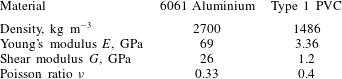
Tabulated material properties of hydrofoil construction materials.

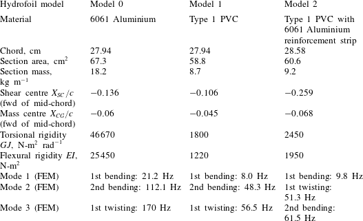
Table 1 lists the material properties of 6061 aluminium and Type 1 PVC. Table 2 gives the mass and section properties of each of the three hydrofoil models. Table 2 also lists the first three in vacuo natural frequencies of each hydrofoil model with the associated normal modes, which were determined by finite element method (FEM) analysis (simulated with a clamped boundary condition at the root) and verified experimentally.
Tabulated physical properties of hydrofoil Model 0, Model 1 and Model 2. The modal frequencies correspond to in vacuo conditions obtained using FEM analysis.

Model 0 was the same hydrofoil described by Harwood et al. (Reference Harwood, Young and Ceccio2016b
), machined from a single piece of aluminium and treated as a rigid specimen. The first flexible hydrofoil (Model 1), was constructed from PVC with outer dimensions identical to those of Model 0. PVC was selected because it is inexpensive, easily machined, has low water absorption, has high ultimate strength relative to most thermoplastics and possesses a density comparable to that of many composites. Thus,
 $\unicode[STIX]{x1D707}$
(defined in (3.1)) is likewise comparable to that of composites in water. The PVC hydrofoil was machined in two halves, symmetric about the mid-thickness plane. Along the plane, two interior channels were machined, into which custom-built shape-sensing spars were installed, as shown in figure 6. Model 2 was simply a modification to Model 1, wherein a strip of 6061 aluminium was affixed to the trailing edge (TE). The aluminium reinforcement strip serves several purposes. First, as shown in figure 6, it moves the shear centre aft by a distance of
 $0.15c$
, increasing the moment arm of the lift force about the foil’s elastic axis (EA). Second, it increases the bending stiffness of the hydrofoil by approximately 60 % and the torsional stiffness by approximately 36 %, as indicated in table 2. The increased flexural rigidity was beneficial for repeated and long-duration testing at highly loaded conditions, particularly those cases described in Part 2 of this paper. It should be noted that the addition of the strip marginally increased the chord length (an increase of 2.3 %), which is judged to be negligible. Therefore, the nominal chord length of
 $c=27.94~\text{cm}$
is used in all cases for non-dimensionalization of loads, immersion depths, etc.
Each of the flexible hydrofoil models was treated as a chordwise-rigid beam in spanwise bending and torsion, with beam-section properties listed in table 2. The shear-centre location, bending stiffness and torsional stiffness were determined by a combination of FEM modelling and experimentation. For the aluminium model (Model 0), an FEM analysis alone was used to estimate section properties. Moving static point loads were applied to Model 1 to experimentally determine the chordwise location of the elastic axis (defined as the locus of sectional shear centres), as well as the effective bending and torsional stiffnesses. These were compared with FEM predictions, in which the Young’s modulus and the Poisson ratio were varied within the manufacturer’s limits until the FEM predictions of shear-centre location and static deflections matched well with experiments (Ward, Harwood & Young Reference Ward, Harwood and Young2018). The resulting material properties are listed in table 1. For Model 2, FEM modelling alone was used to estimate the changes in the sectional properties with the addition of the aluminium strip.
Figure 7 depicts the mounting arrangement, coordinate system and relevant variables. The Cartesian coordinate system was oriented with
 $X$
upstream,
 $Y$
oriented transversely in the direction of positive lift and
 $Z$
following from a right-hand convention. Note that
 $z^{\prime }$
is a local coordinate defined positive downward from the undisturbed free surface. For each of the three models, the hydrofoil was vertically cantilevered and clamped at the root (top) with the tip penetrating to a depth
 $h$
beneath the free surface, where
 $h$
was measured visually against tick marks drawn along the foil span. The root of the foil was affixed to a disk inside the clamping mechanisms, which rotated about the foil’s Z-axis, permitting the foil to be set at a static yaw angle
 $\unicode[STIX]{x1D6FC}$
with respect to the incoming flow;
 $\unicode[STIX]{x1D6FC}$
was set manually using 1 degree indices machined into the yawing disk with an estimated uncertainty of
 $\pm 0.25^{\circ }$
.
(a) Depiction of experimental coordinate system and test variables.
 $U$
is the flow speed,
 $\unicode[STIX]{x1D6FC}$
is the yaw angle (angle of attack),
 $h$
is the immersion of the free tip beneath the undisturbed free surface,
 $c$
is the foil chord and
 $S$
is the cantilevered span of the hydrofoil;
 $z^{\prime }$
is defined as the vertical distance beneath the undisturbed free surface, such that
 $z^{\prime }=h$
at the free tip. (b) Diagram of experimental instrumentation, described in § 4.3.

4.1 University of Michigan towing tank
Experiments with Model 0, Model 1 and Model 2 were carried out in the Physical Modeling Basin at the University of Michigan Marine Hydrodynamics Laboratory, which has dimensions of 110 m (360 ft) long
 $\times$
6.7 m (22 ft) wide
 $\times$
3.05 m (10 ft) deep. It is equipped with a gantry carriage, capable of speeds up to
 $6.1~\text{m}~\text{s}^{-1}$
(
 $20~\text{ft}~\text{s}^{-1}$
). The experimental set-up in the towing tank was described in detail by Harwood et al. (Reference Harwood, Young and Ceccio2016b
), to which the reader is referred for further details.
4.2 Free-surface cavitation channel
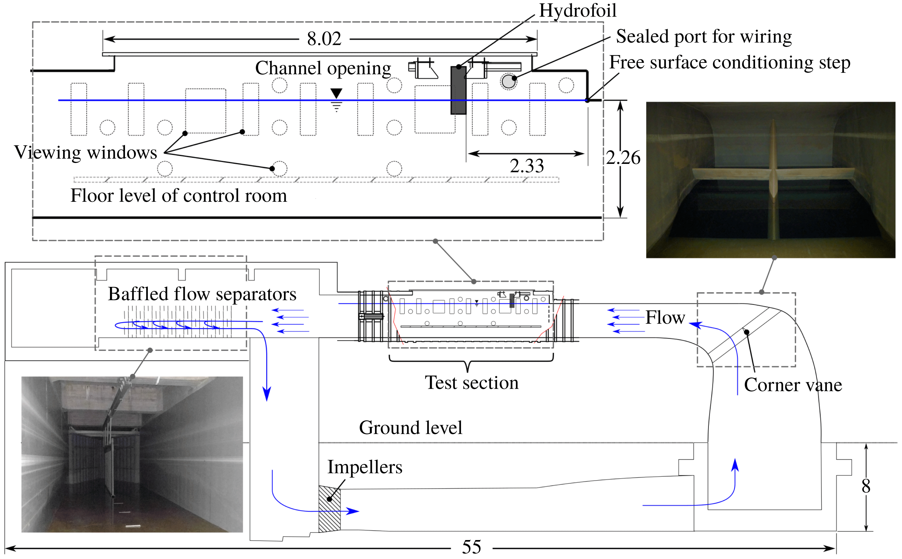
Additional tests of Model 0 and Model 2 were performed in the free-surface, variable-pressure recirculating water channel located at the campus of the Italian National Research Council – Institute of Marine Engineering (CNR INM) in Rome, Italy. The channel has a test section measuring
 $10~\text{m}\times 3.6~\text{m}\times 3~\text{m}$
(
 $L\times W\times D$
) and operates with a water depth of 2.25 m. Before entering the test section, flow passes through a 90
 $^{\circ }$
contracting elbow with a turning vane. Free-surface conditioning is achieved by an inverted backward step at the entrance to the test section.
The coordinate system shown in figure 7 is specific to the CNR-INM channel. It differs from that established by Harwood et al. (Reference Harwood, Young and Ceccio2016b
) for use in the MHL towing tank in that the
 $Z$
-axis is defined positive down (relative to earth), whereas,
 $Z$
was defined positive up during tests in the MHL. The CNR INM flow channel and the MHL towing tank are optimized for observation of the foil from the starboard and port sides, respectively. The use of two coordinate systems permitted positive yaw angles in each facility (opposite in an absolute sense) to be aggregated with a consistent coordinate notation.
The hydrofoil was installed at the centre plane of the section, 2.33 m downstream of the flow conditioning step. A 1 cm thick steel plate was braced and clamped to transversely oriented steel beams to which the rest of the set-up was anchored. The relative locations of the elbow, vane, step and hydrofoil are depicted in figure 8.
Flow through the channel is driven by dual 4-bladed axial impellers that deliver up to 435 kW (584 hp) each, with a maximum flow speed of
 $5~\text{m}~\text{s}^{-1}$
. The flow speed was controlled by prescribing rotation rates of the pump impellers according to a pre-determined calibration curve. Flow visualization (described in § 4.2.1) later confirmed that mean flow velocities had a systematic error of less than 1.5 %.
Elevation sketch of the test section of the cavitation channel at CNR INM. Dimensions are in metres.

It was observed during tests that a non-zero mean flow occurred along the positive
 $Y$
axis, effectively increasing the angle of attack of the vertical hydrofoil. The cause of the cross-flow was not clearly identified, but it is hypothesized to be a standing vortex that occurs at the elbow, which then tilts out of plane when entering the test section. To minimize the bias introduced by the cross-flow, the yaw angle of each test was increased by the cross-flow angle during post-processing to reflect the hydrodynamic angle of attack. More details are given in § 4.2.1.
To investigate the changes in the flow with the onset of vaporous cavitation instead of or in addition to natural ventilation, the ambient pressure of the test section was altered. An airtight cover was placed over the test section and the ambient pressure at the free surface (
 $P_{0}$
) was reduced to modify the vaporous cavitation number. The channel pressure was lowered to a minimum of approximately 40–50 mbar (0.04–0.05 atm). Evacuation of air required between one and four hours, though an additional 12–24 h of de-gassing was found to improve the water quality for visual observation. No changes in the cavitating or ventilated flow topologies were observed with degassing for the cases considered, so testing was performed as usual as soon as the tunnel reached the target pressure.
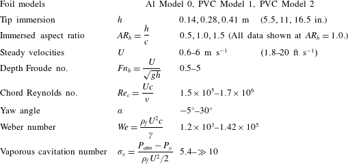
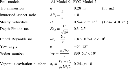
The ranges of test conditions in the towing tank and flow channel are tabulated in tables 3 and 4, respectively. Note that all data described in this work (except where specifically noted) were collected at an immersed aspect ratio of
 $AR_{h}=1.0$
.
Test matrix for towing tank tests.

Test matrix for tests at the CNR INM cavitation channel.

4.2.1 Particle image velocimetry survey of channel flow quality
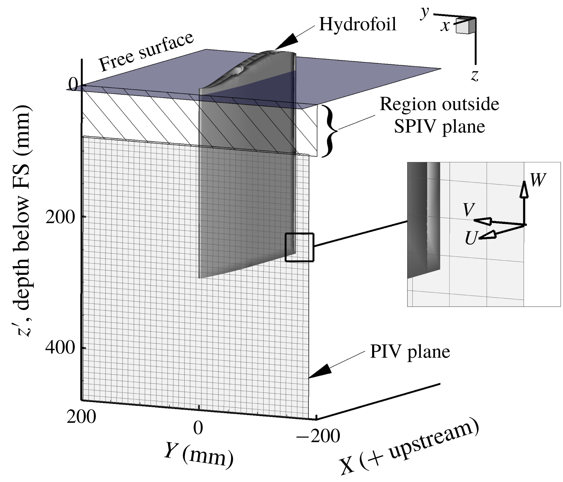
A stereoscopic particle image velocimetry (SPIV) system was used to assess the flow quality in the flow channel. The SPIV test campaign was conducted subsequent to the experimental campaign, with the hydrofoil removed from the channel. Imaging was performed in a transverse plane of the channel at a longitudinal position that would be coincident with the hydrofoil leading edge. The visualization domain consisted of a 40 cm by 40 cm square, centred at the hydrofoil’s free tip (27.9 cm beneath the undisturbed free surface). The visualization plane ended approximately 7.9 cm (3.1 in) beneath the free surface to avoid visual artefacts introduced by the air–water interface.
The particle field motion was computed through an advanced, iterative, multi-pass direct cross-correlation and image deformation method (see Felli, Falchi & Pereira (Reference Felli, Falchi and Pereira2010) for further details). The size of the interrogation windows was 64 pixels by 64 pixels, with a 50 % overlap, resulting in a vector grid spacing of 1 cm by 1 cm. Spatial calibration and velocity vector calculations were performed in the software DaVis® by LaVision. The arrangement is shown in figure 9. Note that the PIV plane utilizes a locally defined left-hand coordinate system. The out-of-plane component is defined as
 $U$
, while the horizontal and vertical in-plane components are respectively
 $V$
and
 $W$
. The local cross-flow angle is defined in the horizontal plane as,
 $$\begin{eqnarray}\unicode[STIX]{x1D6FC}_{in}=\arctan (V/U).\end{eqnarray}$$
Runs were performed at four speeds:
 $1.6~\text{m}~\text{s}^{-1}$
,
 $2.5~\text{m}~\text{s}^{-1}$
,
 $3.3~\text{m}~\text{s}^{-1}$
and
 $4.2~\text{m}~\text{s}^{-1}$
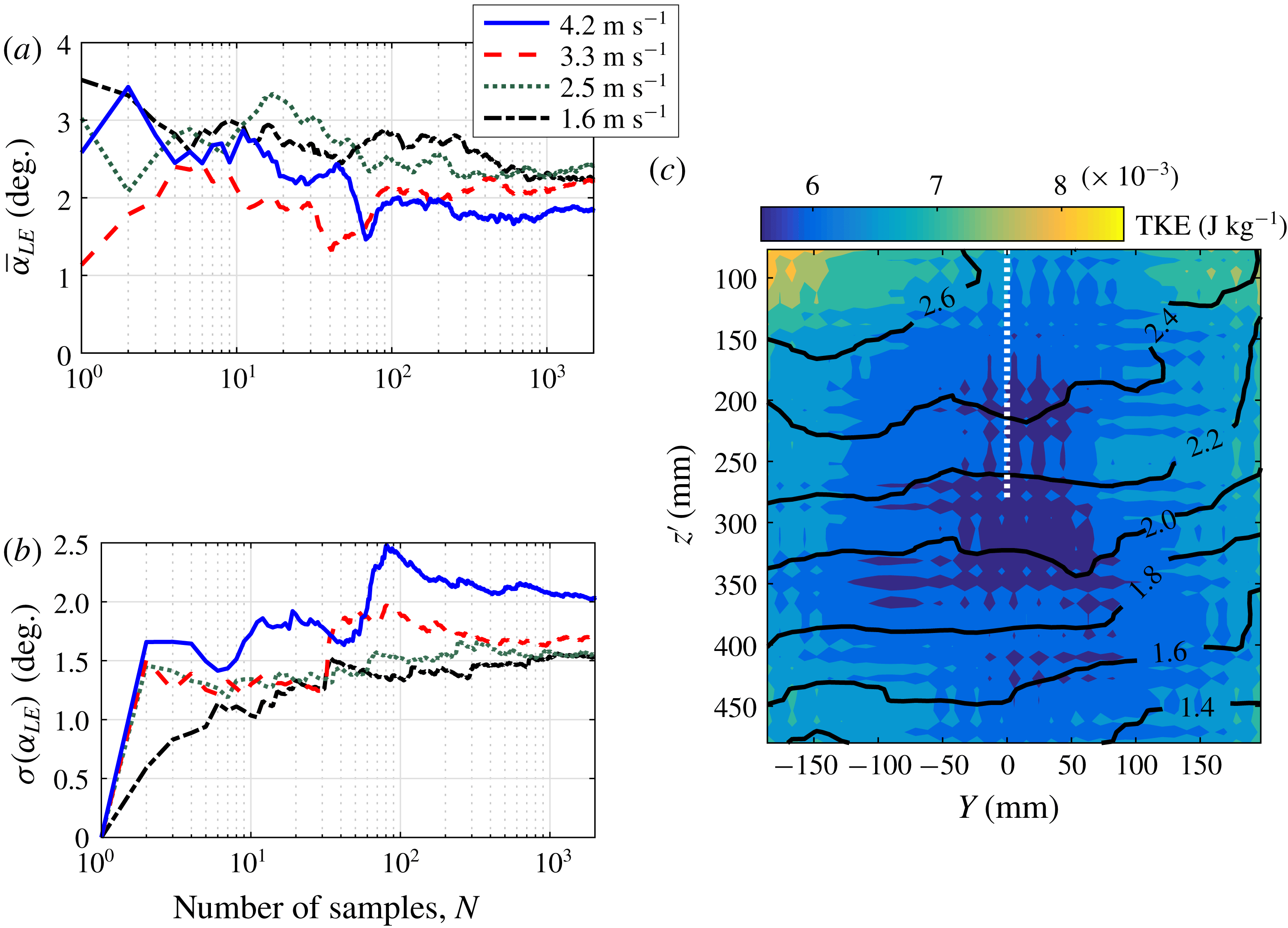
(the primary speeds used during testing of the hydrofoil). At each speed, 2000 frames were recorded at a rate of 10 Hz. Mean cross-flow angles (
 $\unicode[STIX]{x1D6FC}_{LE}$
) are spatial averages of
 $\unicode[STIX]{x1D6FC}_{in}$
taken along the location of the hydrofoil’s leading edge. The convergence of the temporal mean and the temporal standard deviations of
 $\unicode[STIX]{x1D6FC}_{LE}$
, averaged along the foil’s LE location, are shown in figure 10(a,b), showing good convergence of both statistics.
SPIV domain shown relative to the locations of the free surface and hydrofoil. Note that the hydrofoil is shown here for reference, but was removed during the SPIV testing.

Figure 10(c) depicts the time-averaged flow in the PIV plane at
 $2.5~\text{m}~\text{s}^{-1}$
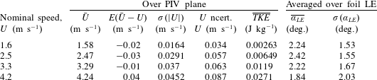
. The axes are shaded by turbulent kinetic energy (TKE) and labelled contour lines indicate the time-averaged local cross-flow angle. The dotted white line indicates the location of the hydrofoil’s leading edge. The contours and shading indicate that the cross-flow increases with proximity to the free surface, while the concavity of the contours and the TKE shading indicate increasing average cross-flow and increasing velocity fluctuations moving away from the centreline. Table 5 reports the mean and standard deviations of the cross-flow angles at the location of the foil’s leading edge (spatially averaged along the white dotted line). The mean cross-flow angle is seen to vary weakly with the flow speed. For each test conducted in the CNR cavitation channel, the effective angle of attack was taken to be the sum of the geometric yaw angle and the cross-flow angle at the corresponding speed, which has a mean value of
 $\unicode[STIX]{x1D6FC}_{LE}=2.18^{\circ }$
. The standard deviations are similar in magnitude to the means, indicating significant unsteadiness in the inflow conditions.
Convergence of (a) the mean and (b) the standard deviation of cross-flow angle. In both cases, the cross-flow angle is spatially averaged along the foil LE. (c) Axes shaded by temporally averaged turbulent kinetic energy for a flow speed of
 $2.5~\text{m}~\text{s}^{-1}$
only. Black contours denote time-averaged horizontal cross-flow angles and the white dashed line indicates the nominal position of the hydrofoil’s leading edge.

Tabulated statistics from PIV survey of the flow channel. The longitudinal velocity component and turbulent kinetic energy are both averaged across all spatial and temporal points. The mean and standard deviations of the cross-flow angle are spatially averaged along the hydrofoil’s leading edge.

4.3 Instrumentation
Major instrumentation components are described individually in the following subsections.
4.3.1 Kinematic measurements
Static and dynamic measurements of the spanwise bending and torsional deformations of the hydrofoil were accomplished using custom-built shape-sensing spars (Harwood et al.
Reference Harwood, Stankovich, Young and Ceccio2016a
,Reference Harwood, Young and Ceccio
b
; Ward, Harwood & Young Reference Ward, Harwood and Young2016; Ward et al.
Reference Ward, Harwood and Young2018). Two independent spars were inserted into the hydrofoil, oriented along the span, separated by a distance of 12.3 cm (0.44
 $c$
) and each equipped with four bending-strain half-bridges, as depicted in figures 6 and 7. The shape-sensing methodology involves the fitting of measured strains by fourth-order polynomials along the two non-coincident lines, which are then twice-integrated with known boundary conditions to yield bending (
 $\unicode[STIX]{x1D6FF}$
) and twisting (
 $\unicode[STIX]{x1D703}$
) displacements along the hydrofoil’s elastic axis. The calibration range of the two-spar set-up is
 $\pm 8~\text{cm}$
in bending (9 % of the hydrofoil span) and
 $\pm 5^{\circ }$
in twisting (defined at the free tip of the hydrofoil). Measurement uncertainties of approximately 2 % (proportional) in bending and
 $0.5^{\circ }$
(absolute) in twisting – both at 95 % confidence levels – make them competitive with optical methods such as digital image correlation (DIC) or marker tracking. Moreover, the sensors do not rely upon optical access and were thus unaffected by visual artefacts such as bubbles or refractive interfaces like the walls of vaporous and/or ventilated cavities. The spars enable the deflected shape of the strut to be measured in situ under static hydrodynamic loads and during dynamic excitation of the hydrofoil up to the sixth natural mode of vibration, which occurs at approximately
 $180~\text{Hz}$
. These deflections may be used for on-line monitoring of mode shapes, inverse load reconstruction (Ward et al.
Reference Ward, Harwood and Young2018) and the reporting of bending and twisting distributions in each of the flow regimes considered. Being zeroth-order sensors, strain gauges are particularly well suited to dynamic measurements, such as the reconstruction of mode shapes in part two of this paper.
The shape sensing is limited by the polynomial-fitting scheme, which fails to capture the effects of large and discontinuous loads – especially those occurring near the free tip of the hydrofoil. It was also found that the strain gauges and signal conditioning suffered from significant drift with prolonged testing in the cavitation channel – probably due to thermal effects. As a result, static deformations were primarily drawn from results obtained in the Michigan Towing Tank, where the amplifiers were frequently re-balanced. A more detailed characterization of the sensor design performance was recently published by Di Napoli et al. (Reference Di Napoli, Young, Ceccio and Harwood2019).
Additionally, one PCB 357B06 charge-type single-axis accelerometer was affixed to the end of each shape-sensing spar with the measurement axis oriented in the
 $Y$
-direction. Signal conditioning was achieved using Bruel and Kjaer model 2635 charge amplifiers and the signals were connected to a pair of Stanford Research Systems SR830 lock-in amplifiers. This arrangement was used to isolate coherent and periodic structural accelerations during experiments – useful for identifying the magnitudes and phases of periodic flow-induced vibrations.
4.3.2 High-speed videography
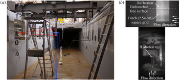
High-speed video was recorded in the cavitation channel using two Photron® brand high-speed cameras (FASTCAM® SA-Series) aimed through windows in the test section – one aimed horizontally at the submerged suction surface and one aimed vertically upward at the foil’s free tip. The camera’s locations relative to the hydrofoil are shown in figure 11(a). Figure 11(b) shows the corresponding fields of view. Both cameras acquired monochrome video at a resolution of
 $1024\times 512$
pixels, 12-bit grey scale and a rate of
 $500$
frames per second. The suction surface was marked with 2.54 cm (1 inch) grid of white paint.
(a) Illustrates the camera perspectives in the cavitation channel at CNR INM. (b) Shows the corresponding fields of view, with the suction surface on top and the hydrofoil free tip viewed from below on the bottom.

4.3.3 Other instrumentation
Forces and moments on the hydrofoil were measured using a six-degree-of-freedom transducer (Omega-190 US-800-6000, manufactured by ATI®) installed at the root of the hydrofoil, with an estimated proportional uncertainty of
 $\pm 2.6\,\%$
for multi-axis loads. Force and moment measurements were used to produce hydrodynamic load coefficients discussed in this manuscript – both steady and dynamic. The model used possesses resonant frequencies of 900–1200 Hz for each of the six measurement axes, so measurements of interest, which were limited to below 200 Hz, were well within the bandwidth of the transducer. However, during unsteady flows, the hydrodynamic loads were conflated with the reaction force of the vibrating hydrofoil, so force measurements alone were insufficient to fully distinguish the hydrodynamic excitation from the response during passive (flow-induced) hydroelastic interactions.
The pressure inside the test section was measured with a dry pressure transducer with an uncertainty of
 $\pm 5~\text{mbar}$
and verified with a mercury manometer with an estimated uncertainty of
 $\pm 1~\text{mbar}$
. The former measurements were used for the calculation of the vaporous cavitation number,
 $\unicode[STIX]{x1D70E}_{v}$
for each trial.
When it was desired to induce ventilation at a specified instant in time, a high-pressure jet of air was injected at the leading edge of the hydrofoil by way of a computer-controlled solenoid valve. This was a modified version of the air-injection system used by Harwood et al. (Reference Harwood, Young and Ceccio2016b ), who showed it to be effective at triggering ventilation in the bi-stable range of flow conditions by creating turbulent, bubbly flow near the hydrofoil’s leading edge, where a small region of flow separation persists near the leading edge.
4.3.4 Data acquisition and processing
Control of the data acquisition system (DAQ), on-line signal processing and logging were performed in National Instruments LABVIEW® software, running on a workstation PC. DAQ hardware consisted of three multifunction input–output data acquisition cards installed into a PXI-e chassis and into the host computer’s PCI bus. All data were digitized at 16 bit depth and recorded at rates of either 500 Hz (CNR INM) or 1000 Hz (University of Michigan). The multiple cards were phase locked to a shared reference clock and triggered to acquire data synchronously. The sample clock was routed as a transistor-transistor logic (TTL) pulse train to the camera controller for synchronization of acquired frames. No anti-aliasing filters were used on the primary DAQ. A second DAQ, manufactured by ProSig® was used to record duplicate data with anti-aliasing filters. Comparison between the data recorded on the two devices revealed that broad-banded process noise resulted in a marginal increase of the noise floor in the unfiltered data. During the modal-analysis phase of testing, however, excitation with the shaker motor led to a pseudo-band-limited output that minimized the effects of aliasing. A positive aspect of the unfiltered measurements is the phase accuracy up to the Nyquist frequency.
It was not possible to bring the flow channel to rest and re-zero the sensors between each acquisition, as was procedure during towing tank tests. Because of this, the shape-sensing spars suffered from some slow drift. This was compounded by the large variability in the channel cross-flow angle indicated in table 5, whereas the quiescent towing tank afforded precise control of the inflow conditions. Data from the flow channel and the towing tank thus possess complementary qualities. Results from the towing tank exhibit low noise and fast convergence of statistics, but acquisitions were of short duration, making these data useful for steady-state results. Those from the flow channel possess higher noise floors, increased sensor drift and slowly convergent statistics, but data were collected for extended periods of time, making these data ideal for frequency-domain analysis and analysis of the hydrofoil dynamics. For the remainder of this work, data from one facility or the other may be omitted from specific results. In all cases, the source of the data will be reported.
5 Static hydroelastic response
This section examines the static hydroelasticity of the hydrofoils and compares the response to that of a reduced-order model. The reduced-order model is presented first, followed by the steady hydrodynamic loads on the rigid and flexible hydrofoils. Scaling of the hydroelastic response and a discussion of static hydroelastic stability conclude the section. Data presented in this section were collected in the Michigan towing tank unless otherwise noted.
5.1 Reduced-order model
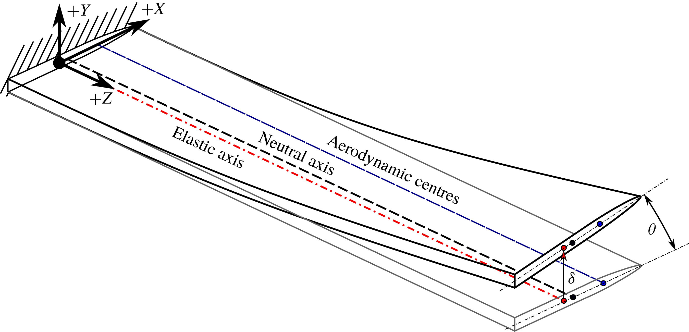
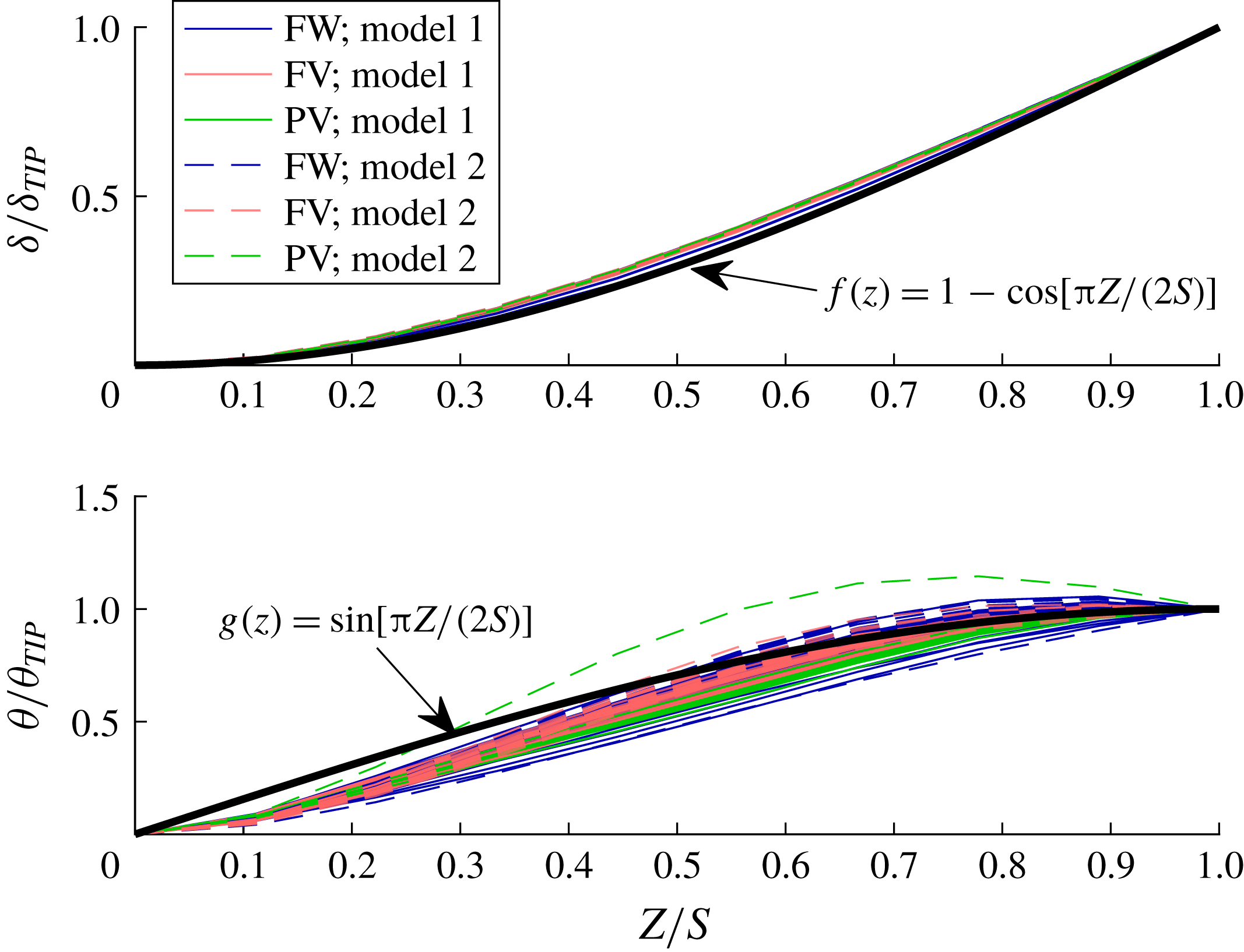
To facilitate a quantitative discussion of the fluid–structure interactions of the hydrofoil, it is useful to introduce a representative 2D-2DOF model. Beginning from the general equations of motion in (3.2) and (3.8), a beam analogy may be adopted, wherein the spanwise flexural and torsional deflections of the hydrofoil are assumed to be decoupled at the elastic axis, similar to the analysis of Bishop & Price (Reference Bishop and Price1979). The beam analogy is depicted in figure 12. By separation of variables, the bending and twisting deflections,
 $\unicode[STIX]{x1D6FF}(z,t)$
and
 $\unicode[STIX]{x1D703}(z,t)$
, respectively, along the spanwise axis
 $z$
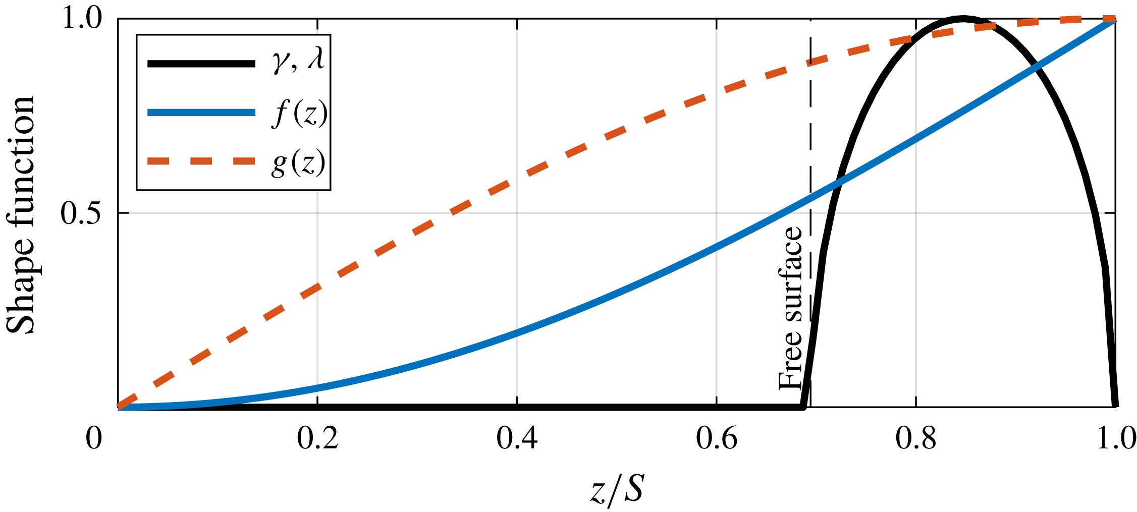
are described by shape functions
 $f(z)$
and
 $g(z)$
as,
 $$\begin{eqnarray}\left.\begin{array}{@{}c@{}}\unicode[STIX]{x1D6FF}(z,t)=\unicode[STIX]{x1D6FF}_{T}(t)f(z);\\ \unicode[STIX]{x1D703}(z,t)=\unicode[STIX]{x1D703}_{T}(t)g(z),\end{array}\right\}\end{eqnarray}$$
where
 $\unicode[STIX]{x1D6FF}_{T}$
and
 $\unicode[STIX]{x1D703}_{T}$
are respectively the tip bending and twisting deflections.
Depiction of the beam analogy adopted for the deflections of the cantilevered hydrofoil. The aerodynamic centres, neutral axis and elastic axis are the respective loci of the sectional centres of pressure, centres of mass and shear centres.

The differential equations of motion for coupled bending and torsion of a beam with constant cross-section become,
 $$\begin{eqnarray}\displaystyle & & \displaystyle \left[\begin{array}{@{}cc@{}}\displaystyle mf(z) & \displaystyle mdg(z)\\ \displaystyle mdf(z) & \displaystyle I_{EA}g(z)\end{array}\right]\left\{\begin{array}{@{}c@{}}\displaystyle \ddot{\unicode[STIX]{x1D6FF}_{T}}\\ \displaystyle \ddot{\unicode[STIX]{x1D703}_{T}}\end{array}\right\}+\left[\begin{array}{@{}cc@{}}\displaystyle -\unicode[STIX]{x1D6FD}\frac{\unicode[STIX]{x2202}^{4}f(z)}{\unicode[STIX]{x2202}z^{4}} & \displaystyle 0\\ \displaystyle 0 & \displaystyle -\unicode[STIX]{x1D6E4}\frac{\unicode[STIX]{x2202}^{2}g(z)}{\unicode[STIX]{x2202}z^{2}}\end{array}\right]\left\{\begin{array}{@{}c@{}}\displaystyle \dot{\unicode[STIX]{x1D6FF}_{T}}\\ \displaystyle \dot{\unicode[STIX]{x1D703}_{T}}\end{array}\right\}\nonumber\\ \displaystyle & & \displaystyle \qquad +\,\left[\begin{array}{@{}cc@{}}\displaystyle -EI\frac{\unicode[STIX]{x2202}^{4}f(z)}{\unicode[STIX]{x2202}z^{4}} & \displaystyle 0\\ \displaystyle 0 & \displaystyle -GJ\frac{\unicode[STIX]{x2202}^{2}g(z)}{\unicode[STIX]{x2202}z^{2}}\end{array}\right]\left\{\begin{array}{@{}c@{}}\displaystyle \unicode[STIX]{x1D6FF}_{T}\\ \displaystyle \unicode[STIX]{x1D703}_{T}\end{array}\right\}\nonumber\\ \displaystyle & & \displaystyle \quad =-\left[\begin{array}{@{}cc@{}}\displaystyle m_{f,\unicode[STIX]{x1D6FF}\unicode[STIX]{x1D6FF}}(z)f(z) & \displaystyle m_{f,\unicode[STIX]{x1D6FF}\unicode[STIX]{x1D703}}(z)g(z)\\ \displaystyle m_{f,\unicode[STIX]{x1D703}\unicode[STIX]{x1D6FF}}(z)f(z) & \displaystyle m_{f,\unicode[STIX]{x1D703}\unicode[STIX]{x1D703}}(z)g(z)\end{array}\right]\left\{\begin{array}{@{}c@{}}\displaystyle \ddot{\unicode[STIX]{x1D6FF}_{T}}\\ \displaystyle \ddot{\unicode[STIX]{x1D703}_{T}}\end{array}\right\}-\left[\begin{array}{@{}cc@{}}\displaystyle c_{f,\unicode[STIX]{x1D6FF}\unicode[STIX]{x1D6FF}}(z)f(z) & \displaystyle c_{f,\unicode[STIX]{x1D6FF}\unicode[STIX]{x1D703}}(z)g(z)\\ \displaystyle c_{f,\unicode[STIX]{x1D703}\unicode[STIX]{x1D6FF}}(z)f(z) & \displaystyle c_{f,\unicode[STIX]{x1D703}\unicode[STIX]{x1D703}}(z)g(z)\end{array}\right]\left\{\begin{array}{@{}c@{}}\displaystyle \dot{\unicode[STIX]{x1D6FF}_{T}}\\ \displaystyle \dot{\unicode[STIX]{x1D703}_{T}}\end{array}\right\}\nonumber\\ \displaystyle & & \displaystyle \qquad -\,\left[\begin{array}{@{}cc@{}}\displaystyle k_{f,\unicode[STIX]{x1D6FF}\unicode[STIX]{x1D6FF}}(z)f(z) & \displaystyle k_{f,\unicode[STIX]{x1D6FF}\unicode[STIX]{x1D703}}(z)g(z)\\ \displaystyle k_{f,\unicode[STIX]{x1D703}\unicode[STIX]{x1D6FF}}(z)f(z) & \displaystyle k_{f,\unicode[STIX]{x1D703}\unicode[STIX]{x1D703}}(z)g(z)\end{array}\right]\left\{\begin{array}{@{}c@{}}\displaystyle \unicode[STIX]{x1D6FF}_{T}\\ \displaystyle \unicode[STIX]{x1D703}_{T}\end{array}\right\}\nonumber\\ \displaystyle & & \displaystyle \qquad +\,\left\{\begin{array}{@{}c@{}}\displaystyle f_{EX}(z)\\ \displaystyle m_{EX}(z)\end{array}\right\}+\left\{\begin{array}{@{}c@{}}\displaystyle f_{\boldsymbol{s}\boldsymbol{f},\boldsymbol{r}}(z)\\ \displaystyle m_{\boldsymbol{s}\boldsymbol{f},\boldsymbol{r}}(z)\end{array}\right\}+\left\{\begin{array}{@{}c@{}}\displaystyle f_{\boldsymbol{u}\boldsymbol{f},\boldsymbol{r}}(z)\\ \displaystyle m_{\boldsymbol{u}\boldsymbol{f},\boldsymbol{r}}(z)\end{array}\right\},\end{eqnarray}$$
where the left-hand side of (5.2) describes the inherent inertial, dissipative and restorative forces of a continuous beam in (decoupled) flexure and torsion and the right-hand side describes the cumulative fluid loading. Here,
 $m$
is the structural mass per unit length,
 $d$
is the distance between the centre of gravity (CG) and the elastic axis (EA), defined as positive when the EA is located upstream of the CG,
 $I_{EA}$
is the sectional mass moment of inertia about the elastic axis,
 $\unicode[STIX]{x1D6FD}$
is the flexural damping,
 $\unicode[STIX]{x1D6E4}$
is the torsional damping and
 $EI$
and
 $GJ$
are the familiar flexural and torsional rigidities, respectively. The quantities
 $m_{f,\ldots }$
,
 $c_{f,\ldots }$
and
 $k_{f,\ldots }$
respectively denote the fluid mass, fluid damping and hydrodynamic stiffness per unit length. In each case, the double subscript indicates that a force is exerted on the degree of freedom indicated in the first subscript by motion in that of the second subscript.
If potential flow is assumed,
 $k_{f,\unicode[STIX]{x1D6FF}\unicode[STIX]{x1D6FF}}=k_{f,\unicode[STIX]{x1D703}\unicode[STIX]{x1D6FF}}=0$
, as there is no fluid restoring force associated with pure bending or pure translation of a lifting surface in an unbounded fluid. For a thin, symmetric airfoil in potential flow, the remaining elements of the hydrodynamic stiffness matrix are given by linear airfoil theory,
 $$\begin{eqnarray}\displaystyle & \displaystyle k_{f,\unicode[STIX]{x1D6FF}\unicode[STIX]{x1D703}}(z)=-a_{0}qc\unicode[STIX]{x1D6FE}(z), & \displaystyle\end{eqnarray}$$
 $$\begin{eqnarray}\displaystyle & \displaystyle k_{f,\unicode[STIX]{x1D703}\unicode[STIX]{x1D703}}(z)=-a_{0}qc^{2}\frac{e_{r}}{2}\unicode[STIX]{x1D706}(z), & \displaystyle\end{eqnarray}$$
 $a_{0}$
is the slope of the sectional lift coefficient plotted against the angle of attack,
 $c$
is the chord length,
 $q=\unicode[STIX]{x1D70C}_{f}U^{2}/2$
is the dynamic pressure and
 $e_{r}$
is the moment arm of the aerodynamic centre (AC) about the EA, normalized by the semi-chord (
 $c/2$
) and defined positive for AC upstream from EA. The function
 $\unicode[STIX]{x1D6FE}(z)$
is a shape function that describes the smooth variation of the sectional lift along the span. Similarly,
 $\unicode[STIX]{x1D706}(z)$
is a shape function describing the variation of the sectional twisting moment about the elastic axis. Both shape functions may be approximated using finite-span airfoil theory (Prandtl Reference Prandtl1918; Helmbold Reference Helmbold1942; Harwood et al.
Reference Harwood, Young and Ceccio2016b
). By extension, the vector
 $\boldsymbol{F}_{\boldsymbol{s}\boldsymbol{f},\boldsymbol{r}}$
becomes,
 $$\begin{eqnarray}\left\{\begin{array}{@{}c@{}}\displaystyle f_{\boldsymbol{s}\boldsymbol{f},\boldsymbol{r}}(z)\\ \displaystyle m_{\boldsymbol{s}\boldsymbol{f},\boldsymbol{r}}(z)\end{array}\right\}=\left[\begin{array}{@{}cc@{}}\displaystyle 0 & \displaystyle -k_{f,\unicode[STIX]{x1D6FF}\unicode[STIX]{x1D703}}(z)\\ \displaystyle 0 & \displaystyle -k_{f,\unicode[STIX]{x1D703}\unicode[STIX]{x1D703}}(z)\end{array}\right]\left\{\begin{array}{@{}c@{}}\displaystyle H\\ \displaystyle \unicode[STIX]{x1D6FC}\end{array}\right\},\end{eqnarray}$$
where
 $\unicode[STIX]{x1D6FC}$
is the initial (undeformed) geometric angle of attack of the hydrofoil, treated here as a rigid-body rotation, and
 $H$
is rigid-body displacement of the lifting surface normal to the flow. As before, it has been assumed that pure translation (
 $H$
) has no effect upon the loading of the hydrofoil.
Substituting (5.3b
) and (5.4) into (5.2), dropping all temporal derivatives and setting external (
 $\boldsymbol{F}_{\boldsymbol{E}\boldsymbol{X}}$
) and unsteady (
 $\boldsymbol{F}_{\boldsymbol{u}\boldsymbol{f},\boldsymbol{r}}$
) forces to zero yields the static equilibrium equation,
 $$\begin{eqnarray}\displaystyle & & \displaystyle \left[\begin{array}{@{}cc@{}}\displaystyle -EI\frac{\unicode[STIX]{x2202}^{4}}{\unicode[STIX]{x2202}z^{4}}f(z) & \displaystyle 0\\ \displaystyle 0 & \displaystyle -GJ\frac{\unicode[STIX]{x2202}^{2}}{\unicode[STIX]{x2202}z^{2}}g(z)\end{array}\right]\left\{\begin{array}{@{}c@{}}\displaystyle \unicode[STIX]{x1D6FF}_{T}\\ \displaystyle \unicode[STIX]{x1D703}_{T}\end{array}\right\}\nonumber\\ \displaystyle & & \displaystyle \quad =\left[\begin{array}{@{}cc@{}}\displaystyle 0 & \displaystyle a_{0}qc\unicode[STIX]{x1D6FE}(z)g(z)\\ \displaystyle 0 & \displaystyle a_{0}qc^{2}\frac{e_{r}}{2}\unicode[STIX]{x1D706}(z)g(z)\end{array}\right]\left\{\begin{array}{@{}c@{}}\displaystyle \unicode[STIX]{x1D6FF}_{T}\\ \displaystyle \unicode[STIX]{x1D703}_{T}\end{array}\right\}+\left[\begin{array}{@{}cc@{}}\displaystyle 0 & \displaystyle a_{0}qc\unicode[STIX]{x1D6FE}(z)\\ \displaystyle 0 & \displaystyle a_{0}qc^{2}\frac{e_{r}}{2}\unicode[STIX]{x1D706}(z)\end{array}\right]\left\{\begin{array}{@{}c@{}}\displaystyle H\\ \displaystyle \unicode[STIX]{x1D6FC}\end{array}\right\}.\end{eqnarray}$$
The right-hand side of (5.5) describes the sectional lift
 $l$
and twisting moment
 $m$
, each per unit span. Integrating only the right-hand side along the geometric span of the hydrofoil
 $z\in [0,S]$
yields the total hydrodynamic lift and moment.
 $$\begin{eqnarray}\displaystyle \left\{\begin{array}{@{}c@{}}\displaystyle L\\ \displaystyle M\end{array}\right\}=\left[\begin{array}{@{}cc@{}}\displaystyle 0 & \displaystyle a_{0}qcSB_{g\unicode[STIX]{x1D6FE}}\\ \displaystyle 0 & \displaystyle a_{0}q\frac{e_{r}}{2}c^{2}SB_{g\unicode[STIX]{x1D706}}\end{array}\right]\left\{\begin{array}{@{}c@{}}\displaystyle \unicode[STIX]{x1D6FF}_{T}\\ \displaystyle \unicode[STIX]{x1D703}_{T}\end{array}\right\}+\left[\begin{array}{@{}cc@{}}\displaystyle 0 & \displaystyle a_{0}qcSB_{\unicode[STIX]{x1D6FE}}\\ \displaystyle 0 & \displaystyle a_{0}qc^{2}\frac{e_{r}}{2}SB_{\unicode[STIX]{x1D706}}\end{array}\right]\left\{\begin{array}{@{}c@{}}\displaystyle H\\ \displaystyle \unicode[STIX]{x1D6FC}\end{array}\right\}. & & \displaystyle\end{eqnarray}$$
The terms involving the structural rigidities are not meaningful when integrated directly, so they have been omitted from (5.6). The
 $B$
factors in (5.6) are the integrals of the respective products of shape functions (denoted by subscripts), normalized by the span; for example,
 $$\begin{eqnarray}B_{f_{1}f_{2}}=\frac{1}{S}\int _{0}^{S}f_{1}(z)f_{2}(z)\,\text{d}z.\end{eqnarray}$$
A list of
 $B$
integrals and their numeric values may be found in appendix A.
To balance the virtual work of the hydrodynamic forces against the strain energies, a Ritz or Galerkin method should be used to cast (5.5) as a 2-DOF model. Multiplying the top and bottom rows of (5.5) by
 $f(z)$
and
 $g(z)$
, respectively, prior to integration yields a second model with principal coordinates of
 $\unicode[STIX]{x1D6FF}_{T}$
and
 $\unicode[STIX]{x1D703}_{T}$
.
 $$\begin{eqnarray}\left[\begin{array}{@{}cc@{}}\displaystyle -EIB_{f^{\prime \prime \prime \prime }f} & \displaystyle 0\\ \displaystyle 0 & \displaystyle -GJB_{g^{\prime \prime }g}\end{array}\right]=\left[\begin{array}{@{}cc@{}}\displaystyle 0 & \displaystyle a_{0}qcSB_{fg\unicode[STIX]{x1D6FE}}\\ \displaystyle 0 & \displaystyle a_{0}q\frac{e_{r}}{2}c^{2}SB_{gg\unicode[STIX]{x1D706}}\end{array}\right]\left\{\begin{array}{@{}c@{}}\displaystyle \unicode[STIX]{x1D6FF}_{T}\\ \displaystyle \unicode[STIX]{x1D703}_{T}\end{array}\right\}+\left[\begin{array}{@{}cc@{}}\displaystyle 0 & \displaystyle a_{0}qcSB_{f\unicode[STIX]{x1D6FE}}\\ \displaystyle 0 & \displaystyle a_{0}qc^{2}\frac{e_{r}}{2}SB_{g\unicode[STIX]{x1D706}}\end{array}\right]\left\{\begin{array}{@{}c@{}}\displaystyle H\\ \displaystyle \unicode[STIX]{x1D6FC}\end{array}\right\}.\end{eqnarray}$$
This may be written compactly in terms of generalized forces as,
 $$\begin{eqnarray}\displaystyle \left[\begin{array}{@{}cc@{}}\displaystyle K_{s,\unicode[STIX]{x1D6FF}} & \displaystyle 0\\ \displaystyle 0 & \displaystyle K_{s,\unicode[STIX]{x1D703}}\end{array}\right]\left\{\begin{array}{@{}c@{}}\displaystyle \unicode[STIX]{x1D6FF}_{T}\\ \displaystyle \unicode[STIX]{x1D703}_{T}\end{array}\right\}=-\left[\begin{array}{@{}cc@{}}\displaystyle 0 & \displaystyle K_{f,\unicode[STIX]{x1D6FF}\unicode[STIX]{x1D703}}\\ \displaystyle 0 & \displaystyle K_{f,\unicode[STIX]{x1D703}\unicode[STIX]{x1D703}}\end{array}\right]\left\{\begin{array}{@{}c@{}}\displaystyle \unicode[STIX]{x1D6FF}_{T}\\ \displaystyle \unicode[STIX]{x1D703}_{T}\end{array}\right\}+\left\{\begin{array}{@{}c@{}}\displaystyle L_{\boldsymbol{s}\boldsymbol{f},\boldsymbol{r}}\\ \displaystyle M_{\boldsymbol{s}\boldsymbol{f},\boldsymbol{r}}\end{array}\right\}. & & \displaystyle\end{eqnarray}$$
Note that the generalized hydrodynamic stiffness matrix in (5.8) is made asymmetric by the flow-induced bend-twist coupling term
 $K_{f,\unicode[STIX]{x1D6FF}\unicode[STIX]{x1D703}}=-a_{0}qcSB_{fg\unicode[STIX]{x1D6FE}}$
. The system is, as a result, non-reciprocal.
Thus far, derivations have remained general, so (5.6) and (5.8) should remain applicable to any slender lifting surface. To proceed, assumptions must now be made that are specific to the surface-piercing hydrofoil under consideration. Chae et al. (Reference Chae, Akcabay and Young2013) and Young et al. (Reference Young, Garg, Brandner, Pearce, Butler, Clarke and Phillips2018a ) proposed that the bending and twisting shape functions on a rectangular cantilevered hydrofoil can be approximated by trigonometric functions,
 $$\begin{eqnarray}\displaystyle & \displaystyle f(z)=1-\cos \left(\unicode[STIX]{x03C0}\frac{z}{2S}\right), & \displaystyle\end{eqnarray}$$
 $$\begin{eqnarray}\displaystyle & \displaystyle g(z)=\sin \left(\unicode[STIX]{x03C0}\frac{z}{2S}\right). & \displaystyle\end{eqnarray}$$
 $g(z)$
that retains the zero-slope condition at the root does yield a better fit to the experimental data. However, differences in shape functions were found to produce little change in the resulting 2D-2DOF model and the fitted function is significantly more complex. Recognizing the limitations in the experimental measurements near the root, it was judged that the simple expression proposed for
 $g(z)$
adequately represents the experimental data.
Comparison of model shape functions (5.9) and experimental data for hydrofoil models and three flow regimes in the Michigan towing tank. Data are plotted for both flexible hydrofoil models at all values of
 $\unicode[STIX]{x1D6FC}$
and
 $Fn_{h}$
. In every case, the spanwise deflections were normalized by the respective value at the tip of the hydrofoil. The proposed model functions adequately capture the experimental measurements.

The shape functions describing the hydrodynamic lift
 $\unicode[STIX]{x1D6FE}(z)$
and moment
 $\unicode[STIX]{x1D706}(z)$
are both approximated as elliptical distributions along only the submerged portion of the hydrofoil, and zero everywhere above the free surface. This choice respects the zero-load boundary conditions at the free surface and the immersed free tip and was shown by Harwood et al. (Reference Harwood, Young and Ceccio2016b
) to adequately reproduce the hydrodynamic loads on the rigid (Model 0) hydrofoil in FW, FV and PV flow regimes. With these assumptions in place, all
 $B$
values are calculable using the expressions in appendix A.
5.2 Hydrodynamic loads
It follows from (5.6) that the global lift and twisting moment may be written as
 $$\begin{eqnarray}\displaystyle L & = & \displaystyle qa_{0}B_{\unicode[STIX]{x1D6FE}}cS\left(\unicode[STIX]{x1D6FC}+\frac{B_{g\unicode[STIX]{x1D6FE}}}{B_{\unicode[STIX]{x1D6FE}}}\unicode[STIX]{x1D703}_{T}\right)\end{eqnarray}$$
 $$\begin{eqnarray}\displaystyle & = & \displaystyle qach(\unicode[STIX]{x1D6FC}+0.964\unicode[STIX]{x1D703}_{T});\end{eqnarray}$$
 $$\begin{eqnarray}\displaystyle M_{Z_{EA}} & = & \displaystyle qa_{0}B_{\unicode[STIX]{x1D706}}c^{2}S\frac{e_{r}}{2}\left(\unicode[STIX]{x1D6FC}+\frac{B_{g\unicode[STIX]{x1D706}}}{B_{\unicode[STIX]{x1D706}}}\unicode[STIX]{x1D703}_{T}\right)\end{eqnarray}$$
 $$\begin{eqnarray}\displaystyle & = & \displaystyle qac^{2}h\frac{e_{r}}{2}(\unicode[STIX]{x1D6FC}+0.964\unicode[STIX]{x1D703}_{T}).\end{eqnarray}$$
 $L$
is the 3-D hydrodynamic lift force. The yawing moment
 $M_{Z_{EA}}$
is defined about the EA and is positive for a nose-up moment. In the preceding equations,
 $a$
is the slope of the 3-D lift coefficient with angle of attack,
 $$\begin{eqnarray}\displaystyle a=a_{0}\frac{S}{h}B_{\unicode[STIX]{x1D706}}, & & \displaystyle\end{eqnarray}$$
which may be modelled using an appropriate 3-D lifting surface theory.
The effective angle of attack is defined as the sum of the undeformed yaw angle and the lift-weighted average of the elastic twist angle along the span (Young et al. Reference Young, Garg, Brandner, Pearce, Butler, Clarke and Phillips2018a ), taken from (5.10) and (5.11) to be,
 $$\begin{eqnarray}\displaystyle \unicode[STIX]{x1D6FC}_{e} & = & \displaystyle \unicode[STIX]{x1D6FC}+\frac{B_{g\unicode[STIX]{x1D706}}}{B_{\unicode[STIX]{x1D706}}}\unicode[STIX]{x1D703}_{T}\nonumber\\ \displaystyle & & \displaystyle \unicode[STIX]{x1D6FC}+0.964\unicode[STIX]{x1D703}_{T}.\end{eqnarray}$$
 $F_{X}$
,
 $F_{Y}$
and
 $M_{Z}$
were measured during experiments using the 6-DOF load cell at the root of the hydrofoil. The lift, drag and yawing moment coefficients are respectively defined as,
 $$\begin{eqnarray}\displaystyle & \displaystyle C_{L}=\frac{F_{Y}}{qch}=\frac{L}{qch}; & \displaystyle\end{eqnarray}$$
 $$\begin{eqnarray}\displaystyle & \displaystyle C_{D}=\frac{-F_{X}}{qch}=\frac{D}{qch}; & \displaystyle\end{eqnarray}$$
 $$\begin{eqnarray}\displaystyle & \displaystyle C_{M}=\frac{M_{Z}}{qc^{2}h}, & \displaystyle\end{eqnarray}$$
 $M_{Z}$
is defined about either the mid-chord position (
 $M_{Z_{0.5c}}$
) or about the elastic axis of the hydrofoil (
 $M_{Z_{EA}}$
) (indicated by the subscript). Hydrodynamic load coefficients are plotted against the initial, undeformed angle of attack
 $\unicode[STIX]{x1D6FC}$
in figure 14, with
 $C_{L}~C_{D}$
and
 $C_{M_{0.5c}}$
(defined with respect to the mid-chord position) plotted respectively in figures 14(a), 14(b) and 14(c).
(a) Values of
 $C_{L}$
, (b)
 $C_{D}$
and (c)
 $C_{M_{0.5c}}$
plotted as functions of the initial (undeformed) yaw angle
 $\unicode[STIX]{x1D6FC}$
. Data shown for Models 0, 1 and 2 at
 $Fn_{h}=3$
,
 $AR_{h}=1.0$
. Hydroelastic coupling results in slightly increased loading for Models 1 and 2, which is most pronounced in
 $C_{L}$
and
 $C_{M_{0.5c}}$
. Coupling is reduced in FV flow because the hydrodynamic twisting moment is reduced.

When the centre of pressure is located forward of the elastic axis (
 $e_{r}>0$
), positive lift on the hydrofoil creates a nose-up twisting moment that increases the effective angle of attack of each hydrofoil section. As a result, the cumulative lift on the hydrofoil will also increase. This is reflected by the inclusion of
 $\unicode[STIX]{x1D703}_{T}$
in (5.10). The degree of coupling differs between the FW and FV flow regimes, as shown most clearly in figure 14(a). In the FW regime, values of
 $C_{L}$
are larger on Model 1 and Model 2 than on Model 0 at equivalent values of
 $\unicode[STIX]{x1D6FC}$
. The difference is small – in some cases less than the experimental uncertainty – but it remains consistent for every angle of attack. Additionally, the upper limit of
 $\unicode[STIX]{x1D6FC}$
for which FW flow is stable, referred to as the stall angle
 $\unicode[STIX]{x1D6FC}_{s}$
, changes from
 $\unicode[STIX]{x1D6FC}_{s}=15^{\circ }$
(Model 0) to
 $\unicode[STIX]{x1D6FC}_{s}=13^{\circ }$
(Model 1, Model 2) as a result of the elastic twist. In FV flow, the flexibility of Models 1 and 2 has no appreciable effects upon
 $C_{L}$
. The lift slope
 $a_{0}$
is smaller in FV flow than in FW flow. As the flow transitions to ventilation, the centre of pressure migrates aft, diminishing the moment arm about the elastic axis,
 $e_{r}$
. The simultaneous reduction in the lift slope and the moment arm elicit a smaller twisting response in FV flow and simultaneously reduce the sensitivity of the lift to the elastic twist.
Figure 14(b) shows a comparison across hydrofoil models of the measured drag coefficient,
 $C_{D}$
. The drag coefficient is comparatively insensitive to the effects of foil flexibility. This signifies that the drag is functionally dependent upon more than the angle of attack or – by extension – the lift. The drag coefficient is a sum of friction, profile, spray and lift-induced components. Lift-induced drag and – to a lesser extent – spray drag are expected to have a dependency upon
 $\unicode[STIX]{x1D6FC}_{e}$
; elastic deflections are too small to significantly alter the friction or profile drag components. As a result, small changes in foil flexibility should not yield significant effects on the aggregate values of
 $C_{D}$
. The drag coefficient is also relatively continuous between the FW and FV flow regimes – a fact proposed by Breslin & Skalak (Reference Breslin and Skalak1959) and Harwood et al. (Reference Harwood, Young and Ceccio2016b
) to occur because the development of FV flow increases profile and spray drag, but decreases frictional and lift-induced drag.
Finally, the yawing moment coefficient
 $C_{M_{0.5c}}$
, measured about mid-chord, is plotted in figure 14(c). Note that, while it is the moment about the elastic axis that appears in (5.11), the location of the elastic axis varies between models, so
 $C_{M_{EA}}$
is exchanged for
 $C_{M_{0.5c}}$
, which is defined about a fixed location. As in the case of the lift coefficient, there is a measurable increase in
 $C_{M_{0.5c}}$
for the flexible hydrofoils, relative to that measured on the rigid hydrofoil, resulting from the positive elastic twist. Once again, the difference is most pronounced in the FW regime, where the elements of the hydrodynamic stiffness matrix in (5.5) are maximized. In the FV regime, the difference effectively vanishes, with the exception of Model 1, which remains consistently larger than Model 0 or Model 2. The reason for this behaviour is not known.
 $C_{L}$
is shown plotted against the effective angle of attack,
 $\unicode[STIX]{x1D6FC}_{e}$
in figure 15(a). Using
 $\unicode[STIX]{x1D6FC}_{e}$
as the independent variable effectively collapses the data in the FW regime, but not in the FV regime. It was posited by Breslin & Skalak (Reference Breslin and Skalak1959), Harwood et al. (Reference Harwood, Young and Ceccio2016b
) and Harwood (Reference Harwood2016) that the lift coefficient is nonlinear in the FV regime because the hydrofoil and the attached cavity together behave as a negatively cambered surface, so that traces of
 $C_{L}$
plotted against
 $\unicode[STIX]{x1D6FC}$
possess a slight negative curvature. Additionally, the weighted average of the twist distribution depends upon the assumed shape factors from which
 $B_{g\unicode[STIX]{x1D706}}$
and
 $B_{\unicode[STIX]{x1D706}}$
are calculated, which suggests that better shape functions may exist for the FV flow regime. For a comparison with theory, equation (5.10) can be non-dimensionalized to yield,
 $$\begin{eqnarray}\displaystyle C_{L} & = & \displaystyle a_{0}\frac{S}{h}B_{\unicode[STIX]{x1D706}}(\unicode[STIX]{x1D6FC}+0.964\unicode[STIX]{x1D703}_{T})\nonumber\\ \displaystyle & = & \displaystyle a(\unicode[STIX]{x1D6FC}+0.964\unicode[STIX]{x1D703}_{T})=a\unicode[STIX]{x1D6FC}_{e}.\end{eqnarray}$$
A theoretical set of curves may be procured by modelling
 $a$
with a suitable 3-D wing theory. For example, the Helmbold equation (Helmbold Reference Helmbold1942) was used to good effect by Harwood et al. (Reference Harwood, Young and Ceccio2016b
) to estimate the 3-D lift slope,
 $a$
, based on the 2-D lift slope
 $a_{0}$
and the submerged aspect ratio
 $AR_{h}$
,
 $$\begin{eqnarray}\displaystyle a=\frac{a_{0}}{\displaystyle \sqrt{1+\left(\frac{a_{0}}{\unicode[STIX]{x03C0}AR_{h}}\right)^{2}}+\frac{a_{0}}{\unicode[STIX]{x03C0}AR_{h}}}. & & \displaystyle\end{eqnarray}$$
Taking values of
 $a_{0}=2\unicode[STIX]{x03C0}~\text{rad}^{-1}$
for FW flow and
 $a_{0}=(\unicode[STIX]{x03C0}/2)~\text{rad}^{-1}$
for FV flow yields the dashed lines plotted in figure 15(a), which agree very well with collapsed data in the FW regime and adequately well in the FV regime.
Figure 15(b) demonstrates that
 $C_{D}$
does not collapse when plotted against
 $\unicode[STIX]{x1D6FC}_{e}$
, which is unsurprising given the insensitivity of the drag to foil flexibility observed in figure 14(b);
 $C_{M}$
is plotted in figure 15(c). When plotted against
 $\unicode[STIX]{x1D6FC}_{e}$
, the FW data collapse, but the FV data still show consistently larger values for Model 1. As in figure 15(a), black dashed lines show theoretical moment coefficients,
 $$\begin{eqnarray}C_{M_{0.5c}}=a\frac{x_{AC}}{c}\unicode[STIX]{x1D6FC}_{e},\end{eqnarray}$$
where
 $x_{AC}=0.3c$
in FW flow and
 $x_{AC}=0.1875c$
(Akcabay & Young Reference Akcabay and Young2014) in FV flow are specified. Thin-airfoil theory posits that the wetted centre of pressure should reside at
 $x_{AC}=0.25c$
, but the non-standard shape of the hydrofoil section is forward loaded, and previous experiments have shown that the centre of pressure is located closer to
 $x_{AC}=0.3c$
.
(a) Values of
 $C_{L}$
, (b)
 $C_{D}$
and (c)
 $C_{M_{0.5c}}$
plotted as functions of the effective angle of attack
 $\unicode[STIX]{x1D6FC}_{e}$
, which includes the lift-weighted average of the elastic twist along the span. Data shown for Models 0, 1 and 2 at
 $Fn_{h}=3$
,
 $AR_{h}=1.0$
. Data in the FW regime are practically collapsed by using
 $\unicode[STIX]{x1D6FC}_{e}$
as the independent variable, while the scatter is increased in the FV data.

The values of
 $C_{L}$
and
 $C_{M}$
are measurably larger for the flexible hydrofoils (Models 1 and 2) than for the rigid Model 0. The differences between Models 1 and 2, however, are less than the experimental uncertainty. For a given flow condition, Models 0, 1 and 2 are expected to share roughly equivalent values of the lift slope
 $a$
and to share a common location for the centre of pressure. Therefore, only
 $e_{r}$
will change in (5.11) – caused by model-to-model variations in the location of the elastic axis – while the centre of pressure remains fixed. This change in moment arm causes the hydrodynamic stiffness to differ between Model 1 and Model 2, while the torsional structural stiffness
 $K_{s,\unicode[STIX]{x1D703}}$
is altered by the presence of the aluminium strip in the latter. Taking the section properties from table 2, one finds that the moment arm of the lift about the EA is 43 % larger on Model 2 than on Model 1 – a result of aft-ward movement of the EA with the addition of the reinforcement strip. However, the torsional rigidity
 $GJ$
of Model 2 is increased by 36 %, relative to that of Model 1. As a result, the ratios of
 $GJ$
to
 $e_{r}$
vary by less than 5 % between Model 1 and Model 2 (with Model 2 having a smaller value), so the twist angle resulting from a lift force acting through the same point will elicit similar twist angles for both Model 1 and Model 2.
5.3 Correlation of hydrodynamic loads with cavitation parameter
The effects of ventilation and vaporous cavitation on the lift and moment coefficients of a rigid hydrofoil are collectively governed by the cavitation parameter
 $\unicode[STIX]{x1D70E}_{c}/\unicode[STIX]{x1D6FC}$
, where
 $\unicode[STIX]{x1D70E}_{c}$
was defined in § 2.1 and
 $\unicode[STIX]{x1D6FC}$
is in radians (Young et al.
Reference Young, Harwood, Miguel, Ward and Ceccio2017). The scaling of a cavity is not directly dependent upon the composition of the cavity itself (air or vapour). To this end, Harwood (Reference Harwood2016) showed that
 $C_{L}$
and
 $C_{M}$
varied smoothly across the FW, PC, PV and FV flow regimes when all were plotted against
 $\unicode[STIX]{x1D70E}_{c}/\unicode[STIX]{x1D6FC}$
.
Let
 $\unicode[STIX]{x1D70E}_{c}$
(from (2.3a
)) be defined at the middle of the immersed span (
 $z^{\prime }=h/2$
) and take the cavity pressure as
 $P_{c}=P_{0}$
for FV flows and
 $P_{c}=P_{v}$
for FW and PC flow. Replacing
 $\unicode[STIX]{x1D6FC}$
with
 $\unicode[STIX]{x1D6FC}_{e}$
, the cavitation parameter is given by,
 $$\begin{eqnarray}\displaystyle & \displaystyle \frac{\unicode[STIX]{x1D70E}_{c}}{\unicode[STIX]{x1D6FC}_{e}}=\frac{\unicode[STIX]{x1D70E}_{v}}{\unicode[STIX]{x1D6FC}_{e}}+\frac{1}{\unicode[STIX]{x1D6FC}_{e}Fn_{h}^{2}}\quad \text{FW and PC flows}, & \displaystyle\end{eqnarray}$$
 $$\begin{eqnarray}\displaystyle & \displaystyle \frac{\unicode[STIX]{x1D70E}_{c}}{\unicode[STIX]{x1D6FC}_{e}}=\frac{1}{\unicode[STIX]{x1D6FC}_{e}Fn_{h}^{2}}\quad \text{FV flows}. & \displaystyle\end{eqnarray}$$
The values of
 $C_{L}$
and
 $C_{M}$
are plotted against
 $\unicode[STIX]{x1D70E}_{c}/\unicode[STIX]{x1D6FC}_{e}$
in figure 16 for all three hydrofoil models. Data are included both from the cavitation channel and from the towing tank. All four of the flow regimes (FW, PV, PC and FV) are represented, each within a relatively well-defined band of
 $\unicode[STIX]{x1D70E}_{c}/\unicode[STIX]{x1D6FC}_{e}$
. While there remains appreciable scatter, the approximately collapsed experimental data are useful for better understanding the behaviours of the several complex multi-phase flows. In the limit as
 $\unicode[STIX]{x1D70E}_{c}/\unicode[STIX]{x1D6FC}_{e}$
approaches infinity, ambient pressures are large and flow speeds and/or angles of attack are vanishingly small. As a result, the flow tends to be steady and single phase. As the speed and/or attack angle increase, FW flow transitions into PV flow, which is characterized by larger force fluctuations. As the angle and/or velocity increase further, the PV flow smoothly transitions to FV flow, which again results in relatively stable flow and steadier hydrodynamic loads. Alternatively, if the ambient pressure is reduced without natural ventilation first taking place, then PC flow is seen to occupy approximately the same band as the PV flow (
 $3\lesssim \unicode[STIX]{x1D70E}_{c}/\unicode[STIX]{x1D6FC}_{e}\lesssim 15$
). If the ambient pressure, angle of attack, or speed are altered to move outside of this range, the PC flow either ceased and the flow returned to the FW regime or the cavitation destabilized and ‘blew out’ to become PV or FV flow;
 $C_{L}$
values peak at intermediate values of
 $1\lesssim \unicode[STIX]{x1D70E}_{c}/\unicode[STIX]{x1D6FC}_{e}\lesssim 20$
, where PV or PC cavities at the leading edge increase the curvature of the flow over the foil sections to produce a virtual camber that is a well-documented effect of partial cavity flows (Acosta Reference Acosta1955). Several outlying data points are visible in the FW flow regime to the far right of both figures, which correspond to flows at low speeds, where the lift and moment coefficients were observed by Harwood et al. (Reference Harwood, Young and Ceccio2016b
) to increase as a result of laminar separation and the mechanism of thin-airfoil stall (Gault Reference Gault1957). Note also that when the velocity approaches zero, even small fluctuations in the measured force are amplified by the vanishingly small denominator of
 $C_{L}$
and
 $C_{M}$
– a fact that explains the growth of the standard deviations and uncertainties for large values of
 $\unicode[STIX]{x1D70E}_{c}/\unicode[STIX]{x1D6FC}_{e}$
.
Measured values of (a)
 $C_{L}$
and (b)
 $C_{M}$
plotted against the generalized cavitation parameter. The FW, PV, PC and FV data practically collapse onto a continuous curve. Data shown for Model 0, Model 1 and Model 2 for both experimental facilities. Filled symbols indicate mean values, coloured bars indicate
 $\pm$
one standard deviation and black bars denote the systematic uncertainty limit estimated by Harwood et al. (Reference Harwood, Young and Ceccio2016b
).

Measured values of (a)
 $C_{L}$
and (b)
 $C_{M}$
, normalized by the mean of the FW values and plotted against the generalized cavitation parameter. The FW, PV, PC and FV data collapse reasonably onto a continuous curve for all three models at all tested values of
 $AR_{h}$
in both experimental facilities.

Perhaps the most striking feature of figure 16 is its resemblance to the 2-D lift and moment coefficient predicted by free-streamline theory for partial cavities (Acosta Reference Acosta1955) and supercavities (Tulin Reference Tulin1953). This similarity suggests that the cavitation – whether vaporous or ventilated – may be separable from the other characteristics of the hydrofoil (e.g. 3-D and free-surface effects) and treated as a modifier to the hydrodynamic loading. Taking the ratio of each plotted value of
 $C_{L}$
and
 $C_{M}$
to the respective value in FW flow yields the proportional change in the hydrodynamic loads with the onset of PV, PC and FV flows. Figure 17 shows the data for
 $AR_{h}=0.5$
,
 $AR_{h}=1.0$
and
 $AR_{h}=1.5$
, each normalized by the respective mean of the FW lift or moment coefficient. The plotted data thus represent nearly 1000 experimental trials, conducted in two facilities, with four flow regimes, on three hydrofoils at varying speeds, immersion depths, yaw angles and ambient pressures. Data for both the lift and moment coefficient ratios suggest correlations, which are approximated by rational polynomial regressions,
 $$\begin{eqnarray}\displaystyle & \displaystyle \frac{C_{L}}{C_{L,FW}}=\frac{\displaystyle \left(\frac{\unicode[STIX]{x1D70E}_{c}}{\unicode[STIX]{x1D6FC}_{e}}\right)^{2}-0.935\left(\frac{\unicode[STIX]{x1D70E}_{c}}{\unicode[STIX]{x1D6FC}_{e}}\right)+1.1}{\displaystyle \left(\frac{\unicode[STIX]{x1D70E}_{c}}{\unicode[STIX]{x1D6FC}_{e}}\right)^{2}-1.535\left(\frac{\unicode[STIX]{x1D70E}_{c}}{\unicode[STIX]{x1D6FC}_{e}}\right)+2.03}; & \displaystyle\end{eqnarray}$$
 $$\begin{eqnarray}\displaystyle & \displaystyle \frac{C_{M}}{C_{M,FW}}=\frac{\displaystyle \left(\frac{\unicode[STIX]{x1D70E}_{c}}{\unicode[STIX]{x1D6FC}_{e}}\right)^{2}+0.0328\left(\frac{\unicode[STIX]{x1D70E}_{c}}{\unicode[STIX]{x1D6FC}_{e}}\right)+1.0721}{\displaystyle \left(\frac{\unicode[STIX]{x1D70E}_{c}}{\unicode[STIX]{x1D6FC}_{e}}\right)^{2}+0.767\left(\frac{\unicode[STIX]{x1D70E}_{c}}{\unicode[STIX]{x1D6FC}_{e}}\right)+3.659}. & \displaystyle\end{eqnarray}$$
Despite significant scatter in figures 16 and 17, data are satisfactorily collapsed, and the correlations reproduce the trends of the cumulative datasets. The utility of the empirical fits lies in the fact that
 $C_{L}$
and
 $C_{M}$
are relatively easy to model in wetted flows using (5.15), (5.16) and (5.17) (see figure 15
a,c). Equations (5.20) and (5.21) allow such predictions to be extended into ventilating and cavitating flows with a reasonable level of accuracy. Examination of figure 17 shows that the greatest variance in load ratios occurs in data for
 $AR_{h}=0.5$
, which suggests that the self-similarity begins to break down as 3-D effects become dominant.
5.4 Scaled steady hydroelastic response
From (5.8), one may derive the ratio of the hydrodynamic virtual work to the elastic strain energy to arrive at the dimensionless scaling expression,
 $$\begin{eqnarray}\displaystyle \frac{\unicode[STIX]{x1D703}_{T}}{\displaystyle \unicode[STIX]{x1D703}_{T}+\frac{B_{g\unicode[STIX]{x1D706}}}{B_{gg\unicode[STIX]{x1D706}}}\unicode[STIX]{x1D6FC}}=\frac{\displaystyle a_{0}c^{2}h\frac{e_{r}}{2}B_{gg\unicode[STIX]{x1D706}}}{-GJSB_{g^{\prime \prime }g}}q, & & \displaystyle\end{eqnarray}$$
which may be combined with (5.12) to yield,
 $$\begin{eqnarray}\displaystyle \frac{\unicode[STIX]{x1D703}_{T}}{\displaystyle \unicode[STIX]{x1D703}_{T}+\frac{B_{g\unicode[STIX]{x1D706}}}{B_{gg\unicode[STIX]{x1D706}}}\unicode[STIX]{x1D6FC}}=\frac{\displaystyle ac^{2}h\frac{e_{r}}{2}\frac{B_{gg\unicode[STIX]{x1D706}}}{B_{\unicode[STIX]{x1D706}}}}{-GJSB_{g^{\prime \prime }g}}q. & & \displaystyle\end{eqnarray}$$
Finally, this may be expressed in terms of generalized forces from (5.8b ) as,
 $$\begin{eqnarray}\displaystyle \frac{\displaystyle \unicode[STIX]{x1D703}_{T}}{\displaystyle \unicode[STIX]{x1D703}_{T}+\frac{B_{g\unicode[STIX]{x1D706}}}{B_{gg\unicode[STIX]{x1D706}}}\unicode[STIX]{x1D6FC}}=\frac{-K_{f,\unicode[STIX]{x1D703}\unicode[STIX]{x1D703}}}{K_{s,\unicode[STIX]{x1D703}}}. & & \displaystyle\end{eqnarray}$$
The preceding equations demonstrate two key characteristics: first, for a given structure at a fixed dynamic pressure
 $q$
, the product of the lift coefficient slope and moment arm is proportional to the ratio of the generalized hydrodynamic stiffness to the generalized structural stiffness in twisting (alternatively the ratio of the fluid disturbing moment to structural elastic restoring moment); second, the ratio of generalized hydrodynamic to structural stiffness varies linearly with the fluid dynamic pressure
 $q$
if the lift slope
 $a$
and the distance from the centre of lift to the elastic axis
 $e_{r}$
remain fixed. The former finding will be used in Part 2 of the paper series to model the hydrodynamic stiffness. Additionally, a value approaching unity would indicate imminent static divergence, i.e. when the fluid disturbing moment negates the structural elastic restoring moment.
Dimensionless twisting deformations at the hydrofoil tip, equivalent to the ratio of generalized hydrodynamic to structural stiffness. The data in the FW and FV flow regimes approach asymptotically linear bounds, presumably corresponding to the limiting cases of fully wetted sections and supercavitating sections everywhere along the span. Dashed lines indicate the theoretical predictions of the scaled twist, using (5.22b ) with values from table 2. Data shown were collected at the Michigan towing tank.

The dimensionless ratio of (5.22c
) is plotted as a function of
 $Fn_{h}^{2}$
, which is proportional to
 $q$
, in figure 18(a) for Model 1 and in figure 18(b) for Model 2. The data in all three flow regimes (FW, PV and FV) are bounded above by the FW data, which lie along a line, and bounded below by the FV data at
 $\unicode[STIX]{x1D6FC}=25^{\circ }$
. It was shown by Harwood et al. (Reference Harwood, Young and Ceccio2016b
) that, as
 $\unicode[STIX]{x1D6FC}$
and
 $Fn_{h}$
increase, the mean cavity length increases, causing both
 $a$
and
 $e_{r}$
to decrease. Alternatively, the same behaviour is predicted by the correlations of figures 16(a) through 17(b).
The upper bound is fixed by the values of
 $e_{r}$
and
 $a_{0}$
for wetted sections in FW flow. As a result, PV data and FV data at small values of
 $\unicode[STIX]{x1D6FC}$
and
 $Fn_{h}$
are roughly coincident with data in the FW regime because a large portion of the hydrofoil’s span remains wetted. As
 $\unicode[STIX]{x1D6FC}$
and/or
 $Fn_{h}$
increase, a greater proportion of the hydrofoil’s span ventilates, and cavities on ventilated sections grow larger. At high speeds and yaw angles, all sections along the hydrofoil span are in the supercavitating regime. Thus, the lower limit is fixed by the values of
 $e_{r}$
and
 $a_{0}$
for supercavitating sections. Flows at low and moderate values of
 $Fn_{h}$
(where the cavity length varies significantly along the span) will fall inside of the triangular regions formed by these upper and lower bounds. The bounds drawn in figure 18(a) are estimated from the plotted data in figure 18, and should not be confused with theoretical predictions. Theoretical predictions were made using values from table 2, equation (5.22b
) and the same limiting values of
 $a_{0}$
and
 $e_{r}$
used in § 5.2 for FW and FV flows. For Model 1, the theory and the experimental data share similar slopes, but the experimental data are systematically higher than the predictions of (5.22b
). The most likely explanation is a small systematic error in the measured twist angle, which is supported by the apparent non-zero intercept of the experimental data. The agreement is much better in the case of Model 2. For both hydrofoils, theoretical and experimental results alike confirm that the generalized hydrodynamic stiffness is reduced by the presence of ventilation.
Dimensionless twist ratio indicating the approach toward static divergence for (a) Model 1 and (b) Model 2. Both cases show experimental data from the towing tank at
 $AR_{h}=1.0$
only. Note that the
 $x$
-intercept corresponds to the inverse square Froude number at the static divergence speed. The FW data describe a linear trend. FV data lie above the FW data, and at a shallower slope, indicating that FV flow delays static divergence through the reduction in hydrodynamic stiffness. Data shown were collected at the Michigan towing tank.

Liu & Young (Reference Liu and Young2010) and Young et al. (Reference Young, Harwood, Miguel, Ward and Ceccio2017) showed that for a 2-D foil section, the following relationship is observed:
 $$\begin{eqnarray}\frac{1}{\unicode[STIX]{x1D703}}=\frac{1}{\unicode[STIX]{x1D6FC}}q_{D}\left(\frac{1}{q}-\frac{1}{q_{D}}\right),\end{eqnarray}$$
where
 $q_{D}$
is the divergence dynamic pressure, indicative of the speed at which
 $(\unicode[STIX]{x1D646}_{S}+\unicode[STIX]{x1D646}_{\boldsymbol{f}})$
becomes singular. In this work, the divergence dynamic pressure is found from (5.11) to be,
 $$\begin{eqnarray}q_{D}=\frac{-GJSB_{g^{\prime \prime }g}}{\displaystyle a_{0}B_{gg\unicode[STIX]{x1D706}}S\frac{e_{r}}{2}c^{2}}.\end{eqnarray}$$
Recognizing that
 $q\propto Fn_{h}^{2}$
for a fixed immersion depth, a version of (5.23) may be derived,
 $$\begin{eqnarray}\frac{\unicode[STIX]{x1D6FC}}{\unicode[STIX]{x1D703}_{T}}=Fn_{h,D}^{2}\frac{B_{gg\unicode[STIX]{x1D706}}}{B_{g}\unicode[STIX]{x1D706}}\left(\frac{1}{Fn_{h}^{2}}-\frac{1}{Fn_{h,D}^{2}}\right),\end{eqnarray}$$
where
 $Fn_{h,D}=U_{D}/\sqrt{gh}$
is the divergence Froude number with
 $U_{D}$
as the divergence speed. As static divergence is approached, the theory suggests that the left-hand side will linearly approach zero. In other words, the
 $x$
-intercept corresponds to the Froude number at the static divergence speed. Figure 19 depicts this relationship for both flexible hydrofoils (towing tank data only). FW data nearly collapse along an approximately affine curve. FV data approach the same curve at low speeds (large values of
 $Fn_{h}^{-2}$
) and depart from the FW data at moderate speeds to describe a curve lying above and possessing a shallower slope than that described by the FW data. This indicates that FV flow delays the onset of static divergence, which is expected because the lift and moment arm are both reduced by ventilation. However, it should be cautioned that unsteady load fluctuations caused by cavity shedding can lead to flow-induced vibrations and even flutter at speed significantly below the divergence condition. Note in figure 19 that the static divergence speed was not reached, which was intentional to avoid damage that could be caused by the foil breaking in the towing tank or cavitation tunnel.
Also included are theoretical values, which come from a combination of (5.24) and (5.25). Theoretical predictions agree with experiments only qualitatively, though the agreement is better for Model 2 than for Model 1, and it improves for both models at higher speeds (smaller values of
 $Fn_{h}^{-2}$
). Reasons offered for the disparity between theory and experiment are the same as those in figure 18 – namely the measurement error in the torsional deflection, which here is made dominant by the fact that
 $\unicode[STIX]{x1D703}_{T}$
resides in the denominator of the ordinate variable. Additionally, a small overestimation of the torsional rigidity or an error in the measured location of the shear centre of Model 1 would contribute to the observed error. Ideally, an extrapolation could be made from each of the flow regimes to predict the respective divergence Froude numbers, ergo the divergence velocities. However, the data presented lie too far from the
 $X$
axis to permit any reasonable extrapolation, so the theoretical curves provide the only prediction. The theoretical predictions are indicated in text callouts.
6 Flow-induced vibration
As described in § 1, flow-induced vibration can result from the unsteady fluid force component
 $\boldsymbol{F}_{\boldsymbol{u}\boldsymbol{f},\boldsymbol{r}}$
caused by modulations in speed or flow direction, cavity shedding, vortex shedding or any other time-varying conditions of the parent flow. The response of the flexible hydrofoil is termed flow-induced vibrations (FIV), and the dynamics of FIV is sensitive to the coherence, period and amplitude of the fluid forces by which they are excited.
Coherent vortex shedding from the hydrofoil in the CNR INM cavitation channel. The hydrofoil was set at a yaw angle of
 $\unicode[STIX]{x1D6FC}=5^{\circ }$
, which becomes a mean hydrodynamic angle of attack of
 $7.2^{\circ }$
when the cross-flow correction is included. From top to bottom:
 $Fn_{h}=1$
,
 $Fn_{h}=1.5$
,
 $Fn_{h}=2$
,
 $Fn_{h}=2.5$
. Details on the right show that the longitudinal distance between counter-rotating vortex pairs is equal to 1.5 times the thickness of the trailing edge, in agreement with Bearman (Reference Bearman1967) and Sallet (Reference Sallet1969). Test performed in CNR INM flow channel.

6.1 Coherent vortex shedding
The corners of the blunt trailing edge on the hydrofoil act as fixed locations for detachment of the flow from the pressure and suction surfaces. Separated flow forms a von Kármán vortex street in the hydrofoil wake, even at Reynolds numbers approaching
 $Re_{c}\approx 10^{6}$
. As an illustration, figure 20 shows vortex shedding in the wake of the hydrofoil during tests at the CNR INM cavitation channel. The hydrofoil was set at a yaw angle of
 $\unicode[STIX]{x1D6FC}=5^{\circ }$
. The cross-flow in the channel increased the hydrodynamic angle of attack to a mean value of
 $\unicode[STIX]{x1D6FC}+\unicode[STIX]{x1D6FC}_{LE}\approx 7.2^{\circ }$
– a yaw angle small enough that the shear flows bounding the wake are produced at the corners of the TE. Vortices shed into the wake entrain limited quantities of air from the free surface and the ventilated base cavity, making them clearly visible as regular striations in the photograph. Detail views are shown on the right-hand side of figure 20, with dashed lines drawn through the vortex cores – note that the sign of the circulation alternates between adjacent vortices. The longitudinal distance between counter-rotating vortex pairs was found to be 1.5 times the trailing edge thickness. This matches the results of Bearman (Reference Bearman1967) and Sallet (Reference Sallet1969), who found that the longitudinal spacing of co-rotating vortices (along the same shear layer) was approximately,
 $$\begin{eqnarray}\unicode[STIX]{x1D6FD}\approx 3h^{\prime },\end{eqnarray}$$
where
 $\unicode[STIX]{x1D6FD}$
is the longitudinal vortex spacing and
 $h^{\prime }$
is the lateral distance between shear layers – taken here to be the thickness of the blunt TE. Bearman (Reference Bearman1967) also showed that the longitudinal vortex spacing remained approximately the same when air was bled into the vortex street via a base cavity. Visual observations from above the free surface also confirmed that the striations in figure 20 are indeed formed by a von Kármán vortex street, and that it remains remarkably coherent at high speeds. Direct measurement of the shedding frequency produced an estimated Strouhal number of,
 $$\begin{eqnarray}St_{t}=f_{vs}\frac{T}{U}=0.275,\end{eqnarray}$$
where
 $f_{vs}$
is the frequency of vortex shedding and
 $T$
is the thickness across the TE of the hydrofoil. The shedding frequency
 $f_{vs}$
was determined using lock-in amplifiers to isolate coherent vibrations measured by the accelerometers at the tips of the shape sensing spars. It is worth noting that the bubbly vortex cores appear to match the slope of the TE cavity from which they detach, so that at the lowest speeds, the portions nearest the free surface deviate from a vertical orientation, so that the vortex street appears tilted. At higher speeds, the vortical wake appears less stable, with increased vortex–vortex interaction and breakdown.
6.2 Disorganized partial cavity shedding
While unsteady cavity shedding was observed, it was generally disorganized because the effects of the free tip and the free-surface induced spanwise variations in cavity length. Figure 21 compares spectra of hydrodynamic yawing moments in FW and PC flows. The PC spectral density is slightly elevated above 20 Hz, but the additional energy content appears fairly broad-banded. No defined peaks are present in the PC spectrum that are not seen in the FW spectrum. Both observations support the observation that partial cavity shedding was aperiodic and disorganized. The spanwise variation in the cavity length led to strongly three-dimensional shedding, with small-scale breakup of the cavity trailing edge. Some modulation of the cavity length was observed on a longer time scale, but it appeared to follow from the variations in velocity or cross-flow angle identified in § 4.2.1. Thus, the PC flow did not appear to contribute substantially to
 $\{f_{\boldsymbol{u}\boldsymbol{f},\boldsymbol{r}}\}$
in (3.8), although the unsteadiness of the partial cavities (regardless of the periodicity) did appear to broaden some spectral peaks as a result of non-stationarity (described in Part 2 of this paper series).
Smoothed power spectral densities of the yawing moment on Model 2 in PC and FW flow at
 $\unicode[STIX]{x1D6FC}=12^{\circ }$
,
 $AR_{h}=1.0$
and
 $Fn_{h}=2.0$
. Wetted natural frequencies are indicated as vertical dashed lines. The peaks are the same in FW and PC flows, i.e. no additional peaks were introduced by cavity shedding. Data from CNR INM flow channel.

Smoothed auto-power spectra of lift
 $(F_{y})$
and bending deflections measured at the intersection of the elastic axis and the free tip
 $(\unicode[STIX]{x1D6FF})$
, shown respectively on the left and the right. Both signals are scaled by
 $Fn_{h}^{-2}$
. The red-shaded region indicates a fairly coherent excitation band containing von Kármán vortex shedding and a speed-dependent machinery vibration. Flow-induced vibrations are apparent at each Froude number, but lock-in with the first mode is especially pronounced, as evident by the amplified peak at approximately 4.5 Hz. Test conditions:
 $\unicode[STIX]{x1D6FC}=-5^{\circ },0^{\circ },5^{\circ }$
(nominal),
 $AR_{h}=1.0$
.

Smoothed auto-power spectra of the yawing moment about mid-chord
 $(M_{Z})$
and the torsional deflections of the hydrofoil measured at the free tip
 $(\unicode[STIX]{x1D703})$
, shown respectively on the left and the right. Both signals are scaled by
 $Fn_{h}^{-2}$
. The yawing excitation and response of modes 2 (first twisting) and 3 (coupled bending and twisting) are made clear. Lock-in with mode 1 occurs at
 $Fn_{h}=-.3$
. Flow-induced vibrations are evident at all other speeds, and are amplified where the excitation band crosses the natural frequencies of modes 2 and 3. Test conditions:
 $\unicode[STIX]{x1D6FC}=-5^{\circ },0^{\circ },5^{\circ }$
(nominal),
 $AR_{h}=1.0$
.

6.3 Frequency content, lock-in and lock-off in fully wetted flow
This subsection demonstrates the flow-induced vibration and resonance (lock-in) of the hydrofoil in fully wetted flow, which is driven primarily by the organized vortex shedding discussed in § 6.1. Figure 22 shows smoothed auto-power spectra of the measured lift (
 $F_{y}$
) and bending deflections (
 $\unicode[STIX]{x1D6FF}$
) at the tip of the hydrofoil, plotted for Froude numbers of
 $0.3\leqslant Fn_{h}\leqslant 2.5$
. Similar results for the normalized spectra of the yawing moment
 $M_{EA}$
and the tip twisting deflections
 $\unicode[STIX]{x1D703}_{T}$
are shown in figure 23. All data were collected in the CNR INM cavitation channel at
 $AR_{h}=1.0$
and nominal yaw angles of
 $\unicode[STIX]{x1D6FC}=5^{\circ }$
,
 $\unicode[STIX]{x1D6FC}=0^{\circ }$
and
 $\unicode[STIX]{x1D6FC}=-5^{\circ }$
. The effective yaw angle varies slightly with the speed, due to the mean cross-flow angle in the tunnel (as reported in § 4.2.1, which adds approximately
 $2.2^{\circ }$
to the nominal angle.) Time-series data are multiplied by
 $Fn_{h}^{-2}$
to remove the scaling of hydrodynamic loads and resulting static deflections with dynamic pressure (power spectra are scaled by
 $Fn_{h}^{-4}$
). The wetted resonant frequencies of the first three modes of the hydrofoil at an immersed aspect ratio of
 $AR_{h}=1.0$
are shown as dotted black lines.
Regular sharp peaks appear in the spectra as a result of AC line noise at 50 Hz, its harmonics and what is hypothesized to be a beat frequency resulting from a non-integer division of the line frequency (approximately 50 Hz) into the sample-clock frequency (exactly 500 Hz). Additionally, peaks at 22 Hz and 44 Hz indicate the fundamental frequency and second harmonic of the vibrating transverse rails to which the test apparatus was mounted.
Of primary interest are two spectral peaks whose frequencies increase linearly with the speed of the flow through the channel. The first is caused by the organized shedding of vortices into a von Kármán wake downstream of the trailing edge, as shown in figure 20. The expected band of vortex-shedding frequencies is indicated at each speed by a shaded region corresponding to Strouhal numbers of
 $0.25\leqslant St_{T}\leqslant 0.3$
. The second peak was traced to the facility machinery – possibly vibration from the impellers and/or drives – and coincided almost exactly with the vortex-shedding frequency at each speed. Unfortunately, the energies of these two dynamic components are conflated together, so as to appear in the spectra as a single peak that increases in frequency as the flow velocity is increased. Further data were collected at each speed after the hydrofoil was removed, using accelerometers and hydrophones to measure the ambient noise and vibration in the channel. The auto-power spectra of these signals are provided in appendix B for completeness.
Forced vibrations (flow induced and mechanical) are evident at all values of
 $Fn_{h}$
, most noticeably in the red-banded regions that indicate a combination of vortex shedding and ambient tunnel vibration. Vortex shedding modifies the pressure distribution on the hydrofoil and, as a result, should be observable as peaks in the force and moment spectra. The resultant structural response to this periodic force is then directly observable in the spectral peaks for the bending and twisting deformations. The spectra of
 $M_{Z_{EA}}$
and
 $\unicode[STIX]{x1D703}$
, in particular, show clearly defined vibration occurring close to the constant Strouhal number of
 $St_{t}=0.25$
.
Where the frequency of vortex shedding is coincident with one of the in situ structural modes, lock-in resonance becomes possible. Two cases of potential lock-in appear in the lift and bending spectra of figure 22, as well as the moment and twisting spectra of figure 23. The first occurs at
 $Fn_{h}=0.3$
, where a sharp peak in figure 22 at the intersection of vortex shedding frequency and the first modal frequency indicates a clear lock-in condition. Direct observations confirmed that cyclic bending motions of the hydrofoil coincided with the shedding of coherent vortices from the trailing edge. The prominence of the peak in the lift and tip bending spectra is consistent with the single-noded bending shape of the mode. A second peak is also visible where the vortex shedding frequency intersects the second modal frequency (first twisting mode) at
 $Fn_{h}=2$
, though it is not as distinct as first-mode lock-in. The force and moment spectra between 30 Hz and 35 Hz show a broader peak with larger side lobes than associated motion spectra – indicating that while the structural mode is certainly being excited, the hydrodynamic excitations are disorganized and probably not locked in with the structural motions. This most easily seen in figure 23, where the twisting mode is registered most effectively by the spectra of the twisting moment and tip torsion. The same behaviour is true at
 $Fn_{h}=2.5$
in figures 22 and 23 both, where the third wetted mode (second bending mode with coupled twisting) is excited by increasingly broad hydrodynamic (and mechanical) excitation band. While regular vortex shedding was observed at higher speeds, the uniformity and coherence of the vortices decreases as the flow speed increases (see figure 20), so it is possible that the vortex shedding at
 $Fn_{h}=2$
and
 $Fn_{h}=2.5$
is not sufficiently coherent to cause proper flow-induced resonance of modes 2 or 3. Moreover, lock-in is only expected to occur if the separation between structural modes is large compared to the band of hydrodynamic excitation frequencies (Kim, Vandiver & Holler Reference Kim, Vandiver and Holler1986; Sarpkaya Reference Sarpkaya1995) – a condition not satisfied by modes 2 and 3.
In figure 23, depicting the moment and twist spectra, lock-in with the first modal frequency is less pronounced, but the lock-off flow-induced vibrations are even more evident than in figure 22. Lock-in with the second mode (the first twisting mode, as reported in table 2) is also easily distinguished.
7 Summary and conclusions
This work is Part 1 of a two-part series on hydroelasticity. This work sought to quantify the hydrodynamic and passive hydroelastic responses of three hydrofoils with varying compliance. One rigid and two flexible hydrofoils were investigated, with tests conducted in the towing tank at the University of Michigan and in the large variable-pressure flow channel at CNR INM – Institute of Marine Engineering.
Fully wetted, fully ventilated and partially ventilated flow regimes were observed as in Harwood et al. (Reference Harwood, Young and Ceccio2016b ). In addition to these three flow regimes, testing in the large variable-pressure flow channel at CNR INM permitted measurements in the partially cavitating flow regime.
A theoretical 2D-2DOF model was developed from a beam representation of the spanwise bending and twisting elastic deformation of the hydrofoil. Shape functions were inferred from simple beam theory and 3-D wing theory. Hydroelastic coupling causes the steady lift and yawing moment coefficients to be larger for the flexible hydrofoils (Models 1 and 2) than for the rigid Model 0 because the centre of lift is upstream of the foil elastic axis, causing a nose-up twist that increases the effective angle of attack and advances transition from FW to FV flow regime slightly. In contrast, the differences between Models 1 and 2 are within the experimental uncertainty bounds. The drag coefficient is relatively unaffected by hydrofoil flexibility. When plotted against the effective angle of attack,
 $\unicode[STIX]{x1D6FC}_{e}$
, which accounts for the foil twist, the experimental lift and moment coefficients nearly collapse across the three hydrofoil models in the FW regime. In the FV regime,
 $\unicode[STIX]{x1D6FC}_{e}$
is less effective at collapsing the data between the three models.
Bending and twisting deflections are proportional to the lift and yawing moment in each flow regime. As a result, structural deflections are much smaller in the FV regime than in the FW regime. By extension, hydrodynamic loads in the FV regime are less sensitive to the effects of hydroelastic coupling, because of the reduction in lift and movement of the centre of lift towards the midchord in FV regime.
The lift and moment coefficients each practically collapse onto curves common to all three hydrofoil models when plotted against the effective cavitation parameter
 $\unicode[STIX]{x1D70E}_{c}/\unicode[STIX]{x1D6FC}_{e}$
. The curves, which are reminiscent of those from 2-D free-streamline theory, are continuous across all four flow regimes. By normalizing the data for each aspect ratio by the respective mean values in the FW regime, data for all three aspect ratios approach collapse, forming curves describing approximately 1000 experimental trials across all values of immersed aspect ratio, Froude number, angle of attack, flow regime, experimental facility and hydrofoil compliance. The resulting correlations are informative and useful in understanding the complex behaviour of the multi-phase flow spanning multiple flow regimes, despite significant scatter.
The ratio
 $\unicode[STIX]{x1D703}_{T}(\unicode[STIX]{x1D703}_{T}+1.036\unicode[STIX]{x1D6FC})^{-1}$
was shown to scale with
 $Fn_{h}^{2}$
for constant lift slope
 $a_{0},a$
and lift eccentricity
 $e_{r}$
. Attached flow in the FW flow regime form one asymptotic boundary, while FV flow at large
 $\unicode[STIX]{x1D6FC}$
and
 $Fn_{h}$
form another. These results are consistent with the numerical study of Akcabay & Young (Reference Akcabay and Young2014). Intermediate yaw angles and Froude numbers, for which spanwise variations in cavity length cause both
 $a_{0}$
and
 $e_{r}$
to vary along the span, fall between these established limits. These ratios are also understood to represent the ratio of generalized hydrodynamic to structural torsional moment. This quantity is important, because it highlights the relative importance of fluid disturbing forces and structural restoring forces. Part 2 of this paper series will investigate this topic in greater detail.
Experimental conditions did not approach static divergence, but results are sufficient to demonstrate that divergence would be delayed by the onset of FV flow, which reduces the hydrodynamic disturbing moment due to reduction in lift and load eccentricity as a result of the centre of lift moving to the midchord. Theoretical predictions corroborate these inferences. It should be noted that although FV delays static divergence, unsteady cavitating flows can lead to flow-induced vibrations and even flutter.
Unsteady cavity shedding was observed in the partially cavitating flow regime, but it was disorganized because of spanwise variations caused by the zero loading at the free surface and tip, and did not excite resonance of the hydrofoil as a result. At small yaw angles, coherent vortex shedding (into a von Kármán street) from the blunt TE of Model 2 was shown to excite flow-induced vibrations at Froude numbers of
 $0.3\leqslant Fn_{h}\leqslant 2.5$
. The distance between vortices shed from the trailing edge was found to remain constant at all speeds, so the vortex-shedding frequency scales linearly with forward speed, leading to an approximately constant Strouhal number of 0.275 based on the foil trailing edge thickness. Lock-in was observed where the frequency of vortex shedding crossed the first resonant frequency of the hydrofoil. The second and third resonant frequencies were excited by hydrodynamic forces not locked in to the hydrofoil’s motions. Peaks elsewhere in the spectra of hydrodynamic force and hydrofoil tip motions indicated non-resonant flow-induced vibration.
This work would benefit from continued efforts to refine the instrumentation and analysis methods presented herein. Refinements of the shape-sensing spars should be pursued to enable better resolution of spanwise bending and twisting deformations, which, along with pressure measurements and flow visualization, could be used to formulate more-accurate reduced-order models. Data collected in the large variable-pressure flow channel at CNR INM lacked stationarity in the inflow conditions, which was exacerbated by the inability to zero-out all sensors between runs. If future trials are performed in a similar facility, careful attention should be paid to experimental planning that allows sensor drift to be quantified or negated. An interesting topic for future investigation is the passive hydroelastic response of surface-piercing hydrofoils in waves. Surface waves act both to excite the hydrofoil and to modulate its fluid system parameters, which may promote rich nonlinear FSI responses, and are discussed in more details in Young et al. (Reference Young, Yoon, Wright and Harwood2018c ).
Although the degree of hydroelastic coupling demonstrated in this work remained moderate, the results herein have shown that hydroelasticity is a significant consideration in the design of safe, efficient and controllable lifting surfaces. Designers of compliant lifting surfaces should remain cognizant of static divergence and undesirable flow-induced vibration. Additionally, it is important to consider the risk of externally induced resonance or dynamic flutter. Doing so requires consideration of resonant frequencies and effective damping across a wide range of flow regimes and conditions. To date, such parameters have remained challenging to quantify in hydraulic flows, let alone cavitating or ventilating flows. Part 2 of this paper focuses upon the identification of modal quantities for a fluid–structure system in a variety of multi-phase flows in order to gain insight into the dynamical response and stability of a surface piercing hydrofoil.
Acknowledgements
The authors gratefully acknowledge the support from the Office of Naval Research and Dr K.-H. Kim under ONR grant number N00014-16-1-2433. The authors thank the National Research Council of Italy – Institute of Marine Engineering (CNR INM) for the facility time and assistance when collecting measurements in the large variable-pressure flow channel.
Appendix A. Shape function integrals
Recall that
 $Z$
is defined positive down, measured from the foil root;
 $z^{\prime }$
is defined positive down, measured from the undisturbed water level. Thus,
 $$\begin{eqnarray}\displaystyle & \displaystyle z^{\prime }=z+h-S, & \displaystyle\end{eqnarray}$$
 $$\begin{eqnarray}\displaystyle & \displaystyle \frac{z^{\prime }}{h}=\left(\frac{z}{S}+\frac{AR_{h}-AR_{G}}{AR_{G}}\right)\frac{AR_{G}}{AR_{h}}. & \displaystyle\end{eqnarray}$$
The elliptical shape factor used to approximate the lift and moment distributions on the hydrofoil is
 $$\begin{eqnarray}\displaystyle & \displaystyle \unicode[STIX]{x1D6FE}(z)=\left\{\begin{array}{@{}ll@{}}0,\quad & z^{\prime }\leqslant 0,\\ \displaystyle \sqrt{1-\left(2\left[\left(\frac{z}{S}+\frac{AR_{h}-AR_{G}}{AR_{G}}\right)\frac{AR_{G}}{AR_{h}}\right]-1\right)^{2}},\quad & z^{\prime }>0,\end{array}\right. & \displaystyle\end{eqnarray}$$
 $$\begin{eqnarray}\displaystyle & \displaystyle \unicode[STIX]{x1D706}(z)=\unicode[STIX]{x1D6FE}(z). & \displaystyle\end{eqnarray}$$
The bending and twisting shape factors are respectively,
 $$\begin{eqnarray}\displaystyle & \displaystyle f(z)=1-\cos \left(\unicode[STIX]{x03C0}\frac{z}{2S}\right), & \displaystyle\end{eqnarray}$$
 $$\begin{eqnarray}\displaystyle & \displaystyle g(z)=\sin \left(\unicode[STIX]{x03C0}\frac{z}{2S}\right). & \displaystyle\end{eqnarray}$$
All of the preceding shape functions are plotted in figure 24.
Shape functions
 $f(z)$
,
 $g(z)$
,
 $\unicode[STIX]{x1D6FE}(z)$
and
 $\unicode[STIX]{x1D706}(z)$
plotted along the span of the hydrofoil. The position of the free surface is indicated by the dashed black line.

Smoothed power spectral densities of hydrophone measurements in the channel. Measurements were made with the hydrofoil removed. For reference, red shaded regions indicate the frequency band in which vortex shedding was observed with the hydrofoil installed.

The
 $B$
integrals are defined below. The numerical of each integral are given for the case when
 $AR_{h}=1$
and
 $AR_{G}=3.277$
 $$\begin{eqnarray}\displaystyle & \displaystyle B_{g\unicode[STIX]{x1D6FE}}=\frac{1}{S}\int _{0}^{S}g(z)\unicode[STIX]{x1D6FE}(z)\,\text{d}z=0.231, & \displaystyle\end{eqnarray}$$
 $$\begin{eqnarray}\displaystyle & \displaystyle B_{g\unicode[STIX]{x1D706}}=\frac{1}{S}\int _{0}^{S}g(z)\unicode[STIX]{x1D706}(z)\,\text{d}z=0.231, & \displaystyle\end{eqnarray}$$
 $$\begin{eqnarray}\displaystyle & \displaystyle B_{\unicode[STIX]{x1D6FE}}=\frac{1}{S}\int _{0}^{S}\unicode[STIX]{x1D6FE}(z)\,\text{d}z=0.24, & \displaystyle\end{eqnarray}$$
 $$\begin{eqnarray}\displaystyle & \displaystyle B_{\unicode[STIX]{x1D706}}=\frac{1}{S}\int _{0}^{S}\unicode[STIX]{x1D706}(z)\,\text{d}z=0.24, & \displaystyle\end{eqnarray}$$
 $$\begin{eqnarray}\displaystyle & \displaystyle B_{f^{\prime \prime \prime \prime }f}=\frac{1}{S}\int _{0}^{S}f(z)\frac{\text{d}^{4}}{\text{d}z^{4}}f(z)\,\text{d}z=-0.832, & \displaystyle\end{eqnarray}$$
 $$\begin{eqnarray}\displaystyle & \displaystyle B_{g^{\prime \prime }g}=\frac{1}{S}\int _{0}^{S}g(z)\frac{\text{d}^{2}}{\text{d}z^{2}}g(z)\,\text{d}z=-1.234, & \displaystyle\end{eqnarray}$$
 $$\begin{eqnarray}\displaystyle & \displaystyle B_{fg\unicode[STIX]{x1D6FE}}=\frac{1}{S}\int _{0}^{S}g(z)\unicode[STIX]{x1D6FE}(z)\,\text{d}z=0.177, & \displaystyle\end{eqnarray}$$
 $$\begin{eqnarray}\displaystyle & \displaystyle B_{g\unicode[STIX]{x1D706}}=\frac{1}{S}\int _{0}^{S}g(z)\unicode[STIX]{x1D706}(z)\,\text{d}z=0.223, & \displaystyle\end{eqnarray}$$
 $$\begin{eqnarray}\displaystyle & \displaystyle B_{f\unicode[STIX]{x1D6FE}}=\frac{1}{S}\int _{0}^{S}\unicode[STIX]{x1D6FE}(z)\,\text{d}z=0.183, & \displaystyle\end{eqnarray}$$
 $$\begin{eqnarray}\displaystyle & \displaystyle B_{g\unicode[STIX]{x1D706}}=\frac{1}{S}\int _{0}^{S}\unicode[STIX]{x1D706}(z)\,\text{d}z=0.231. & \displaystyle\end{eqnarray}$$
Appendix B. Ambient noise and vibration in flow channel
Tests were conducted in the CNR INM flow channel without the hydrofoil installed to determine the ambient noise and vibration of the facility during operation. Figure 25 shows the power spectral density of the pressures measured with three hydrophones – one near field, one far field and one above the water surface. Figure 26 shows the power spectral densities of longitudinal and vertical accelerations measured on the transverse beam used to support the hydrofoil model during testing. Both figures show an excitation that increases in frequency with increasing flow speeds.
Smoothed power spectral densities of facility accelerations. Measurements were made with the hydrofoil removed. For reference, red shaded regions indicate the frequency band in which vortex shedding was observed with the hydrofoil installed.

Nomenclature
-
 $a$
Slope of 3-D lift coefficient with angle of attack
-
$a_{0}$
Slope of sectional lift coefficient with angle of attack
-
$U_{D}$
Divergence speed
-
$U$
Free-stream velocity
-
$c$
Chord
-
$e$
Dimensionless distance from elastic axis to centre of pressure,
$\displaystyle \frac{X_{EA}-X_{CP}}{c}$
-
$EI$
Flexural rigidity (spanwise flexure)
-
$f$
Cyclic frequency
-
$f(z)$
Beam bending shape function
-
$g$
Gravitational acceleration
-
$g(z)$
Beam torsion shape function
-
$GJ$
Torsional rigidity (spanwise torsion)
-
$h$
Immersion depth
-
$L,D,M$
3-D lift, drag and moment (
$F_{Y}$
,
$-F_{X}$
,
$M_{Z}$
)-
$l,d,m$
2-D section lift, drag and moment
-
$L_{c}$
Cavity length
-
$P$
Local pressure
-
$P_{\infty }$
Free-stream pressure
-
$P_{atm}$
Atmospheric pressure (101 kPa)
-
$P_{0}$
Ambient pressure at the free surface
-
$P_{c}$
Cavity pressure
-
$P_{v}$
Fluid vapour pressure
-
$S$
Span
-
$T$
Maximum foil thickness
-
$z^{\prime }$
Distance measured downward from the free surface
-
$\unicode[STIX]{x1D6FC}$
Geometric angle of attack or yaw angle
-
$\unicode[STIX]{x1D6FC}_{in}$
Cross-flow angle, computed from local velocities
-
$\unicode[STIX]{x1D6FC}_{LE}$
Cross-flow angle, averaged along leading edge
-
$\unicode[STIX]{x1D6FC}_{e}$
Effective angle of attack, including elastic twist
-
$\unicode[STIX]{x1D6FD}$
Flexural damping
-
$\bar{\unicode[STIX]{x1D6F7}}$
Angle of straight-line fit through cavity-closure line
-
$\unicode[STIX]{x1D6FF}$
Spanwise bending deflection
-
$\unicode[STIX]{x1D6E4}$
Torsional damping
-
$\unicode[STIX]{x1D6FE}(z)$
Shape function of spanwise sectional lift
-
$\unicode[STIX]{x1D706}(z)$
Shape function of spanwise sectional twisting moment
-
$\unicode[STIX]{x1D708}$
Fluid kinematic viscosity
-
$\unicode[STIX]{x1D6F7}$
Local angle of cavity-closure line
-
$\unicode[STIX]{x1D703}$
Spanwise twisting deflection
-
$k_{\cdots }$
Local stiffness
-
$K_{\cdots }$
Generalized stiffness
-
$C_{D}$
3-D drag coefficient,
$\displaystyle \frac{D}{\unicode[STIX]{x1D70C}_{f}chU^{2}/2}$
-
$C_{L}$
3-D lift coefficient,
$\displaystyle \frac{L}{\unicode[STIX]{x1D70C}_{f}chU^{2}/2}$
-
$C_{M}$
3-D moment coefficient,
$\displaystyle \frac{M}{\unicode[STIX]{x1D70C}_{f}c^{2}hU^{2}/2}$
-
$Fn_{h}$
Depth-based Froude number,
$\displaystyle \frac{U}{\sqrt{gh}}$
-
$\unicode[STIX]{x1D707}$
Solid-to-fluid mass ratio,
$\displaystyle \sqrt{\frac{4m}{\unicode[STIX]{x1D70C}_{f}\unicode[STIX]{x03C0}c^{2}}}$
-
$Re_{c}$
Chord-based Reynolds number,
$\displaystyle \frac{Uc}{\unicode[STIX]{x1D708}}$
-
$\unicode[STIX]{x1D70C}_{f}$
Fluid density
-
$\unicode[STIX]{x1D70E}_{c}$
General cavitation index,
$\displaystyle \frac{P_{\infty }-P_{c}}{\unicode[STIX]{x1D70C}_{f}U^{2}/2}$
-
$\unicode[STIX]{x1D70E}_{v}$
Vaporous cavitation index,
$\displaystyle \frac{P_{0}-P_{v}}{\unicode[STIX]{x1D70C}_{f}U^{2}/2}$
-
$AR_{h}$
Immersed aspect ratio,
$h/c$
-
$AR_{G}$
Geometric aspect ratio,
$S/c$
-
$St_{x}$
Strouhal number, based on length scale
$x$
,
$\displaystyle \frac{fx}{U}$
-
$\unicode[STIX]{x1D63E}_{\boldsymbol{f}}$
Fluid damping matrix
-
$\unicode[STIX]{x1D63E}_{\boldsymbol{s}}$
Structural damping matrix
-
$\unicode[STIX]{x1D63E}$
Consolidated/effective damping matrix
-
$\unicode[STIX]{x1D646}_{\boldsymbol{f}}$
(Hydrodynamic) fluid stiffness matrix
-
$\unicode[STIX]{x1D646}_{\boldsymbol{s}}$
Structural stiffness matrix
-
$\unicode[STIX]{x1D646}$
Consolidated/effective stiffness matrix
-
$\unicode[STIX]{x1D648}_{\boldsymbol{f}}$
Fluid mass matrix
-
$\unicode[STIX]{x1D648}_{\boldsymbol{s}}$
Structural mass matrix
-
$\unicode[STIX]{x1D648}$
Consolidated/effective mass matrix
-
$\boldsymbol{F}_{\boldsymbol{E}\boldsymbol{X}}$
Vector of external forces
-
$\boldsymbol{F}_{\boldsymbol{f}\boldsymbol{l}}$
Vector of fluid forces
-
$\boldsymbol{F}_{\boldsymbol{s}\boldsymbol{f},\boldsymbol{r}}$
Steady fluid forces on an equivalent rigid structure
-
$\boldsymbol{F}_{\boldsymbol{u}\boldsymbol{f},\boldsymbol{r}}$
Unsteady fluid excitation forces on equivalent rigid structure
-
$\boldsymbol{X}_{\mathbf{0}}$
Rigid-body attitude of structure, measured relative to the zero-load attitude
-
$\boldsymbol{X}$
Vector of bending and twisting displacements