
 ϵk=O(1)
 κ≫1



1. Introduction
Instabilities of internal gravity–inertial waves in rotating stratified fluids are of great geophysical interest and have been studied extensively. A large body of prior work is devoted to time-harmonic plane waves, which are exact (nonlinear) flow states (irrespective of the spatial profile) in an unbounded, inviscid, uniformly stratified (constant buoyancy frequency) Boussinesq fluid under the
 $f$
-plane approximation. Naturally, linear stability analysis of such time-periodic basic flows rests on Floquet theory.
Using Floquet theory, Mied (Reference Mied1976) examined the stability of propagating pure gravity plane waves with sinusoidal profile to two-dimensional perturbations. He pointed out that at small wave amplitude, instability arises due to resonant triad interactions of the basic state with subharmonic perturbations. Later, comprehensive Floquet stability analyses of propagating sinusoidal gravity–inertial plane waves to three-dimensional perturbations confirmed this triad resonance instability (TRI) in the small-amplitude limit, and also revealed a host of other instability mechanisms that arise at finite amplitude (e.g. see Yau et al. Reference Yau, Klaassen and Sonmor2004).
A particular form of TRI, where the two subharmonic perturbations have half the basic-wave frequency and very fine wavelength, is referred to as parametric subharmonic instability (PSI) (e.g. see McComas & Bretherton Reference McComas and Bretherton1977; Staquet & Sommeria Reference Staquet and Sommeria2002). This mechanism has attracted considerable interest as it permits transfer of energy to smaller scales and thus may contribute to the dissipation of oceanic internal waves (Hibiya et al. Reference Hibiya, Nagasawa and Niwa2002; MacKinnon & Winters Reference MacKinnon and Winters2005; Young et al. Reference Young, Tsang and Balmforth2008; Onuki & Hibiya Reference Onuki and Hibiya2019).
More recent work focused on instabilities of propagating gravity–inertial plane waves with locally confined spatial profile (see the review by Dauxois et al. Reference Dauxois, Joubaud, Odier and Venaille2018). Such wave beams play a part in the barotropic-to-baroclinic tidal energy conversion in oceans (Lamb Reference Lamb2004; Cole et al. Reference Cole, Rudnick, Hodges and Martin2009; Johnston et al. Reference Johnston, Rudnick, Carter, Todd and Cole2011) and also in the development of thunderstorms in the atmosphere (Fovell et al. Reference Fovell, Durran and Holton1992). Compared with sinusoidal plane waves, Floquet stability analysis of wave beams is computationally more challenging (Kataoka & Akylas Reference Kataoka and Akylas2013; Onuki & Tanaka Reference Onuki and Tanaka2019; Fan & Akylas Reference Fan and Akylas2021), and the finite beam width adds new physics.
Specifically, in regard to PSI, the finite beam width is stabilising, as small-scale subharmonic perturbations are wavepackets that travel with their group velocity so they have limited time to extract energy from the underlying wave. This suppression of PSI was suggested by approximate models (Bourget et al. Reference Bourget, Scolan, Dauxois, Le Bars, Odier and Joubaud2014; Karimi & Akylas Reference Karimi and Akylas2014) and also was confirmed by solving the Floquet stability eigenvalue problem for propagating wave beams of small peak amplitude subject to two-dimensional small-scale perturbations (Fan & Akylas Reference Fan and Akylas2021).
An alternative approach to studying small-scale instabilities of inviscid flows is based on the WKB approximation. The idea is to assume initial disturbances in the form of localised short-scale wavepackets, and derive (approximate) equations for the evolution of the wavepacket wavevector and amplitude as the disturbance is advected by the basic flow. These transport equations are ordinary differential equations on fluid particle paths in the underlying flow, and a flow is unstable if there are solutions unbounded in time (Friedlander & Vishik Reference Friedlander and Vishik1991; Lifschitz & Hameiri Reference Lifschitz and Hameiri1991).
This so-called ‘local’ stability approach has been applied to propagating and standing gravity–inertial plane waves with sinusoidal profile (e.g. see Miyazaki & Adachi Reference Miyazaki and Adachi1998; Ghaemsaidi & Mathur Reference Ghaemsaidi and Mathur2019; Abhiram & Mathur Reference Abhiram and Mathur2024; and references therein). As particle paths are closed trajectories (ellipses) traversed at the period of the basic wave, local stability analysis leads to a ‘reduced’ Floquet problem based on the transport equations, and instability hinges on computing the corresponding Floquet exponents. Apart from its relative simplicity and intuitive appeal, local stability analysis also does not seem to restrict the basic-wave amplitude. In the small-amplitude limit, in particular, it has been suggested that local stability recovers PSI of gravity (Ghaemsaidi & Mathur Reference Ghaemsaidi and Mathur2019) and inertial (Abhiram & Mathur Reference Abhiram and Mathur2024) propagating sinusoidal waves.
However, as local stability analysis relies on the WKB approximation, it is natural to ask: (i) if/how the local approximation can be deduced from the exact (‘global’) stability analysis based on Floquet theory; (ii) how short the perturbations should be for local stability to be valid; and (iii) what physics, if any, is lost by resorting to this approximate treatment of short-scale instabilities.
The present paper addresses these open questions for the case of gravity–inertial plane waves with general spatial profile. The key is recasting the linear stability equations in Lagrangian coordinates following particle paths in the basic flow. This eliminates certain terms that become unbounded (‘secular’) in the short-scale limit due to the advection of the perturbations by the underlying wave. Then, introducing normal modes – without making any assumption regarding their length scale
 $1/k$
and/or the basic-wave amplitude
 $\epsilon$
– establishes the connection between the global and local stability analyses. Specifically, the constant wavevector of such ‘Lagrangian’ modes translates to a time-periodic ‘Eulerian’ wavevector that coincides with the local wavevector of wavepackets in local stability analysis. Furthermore, in the (exact) equations for the amplitudes of these modes, the spatial scale of the perturbations manifests in certain
 $\mathcal{O}(1/k)$
terms. Thus the (approximate) transport equations of local stability are obtained by simply dropping these terms, assuming
 $1/k\rightarrow 0$
.
The
 $\mathcal{O}(1/k)$
terms ignored in local stability account for the effects of dispersion on the amplitudes (envelopes) of the assumed short-scale localised wavepackets. Intuitively, these effects are expected to oppose the (potentially destabilising) interaction of such wavepackets with the basic wave, suggesting that local stability provides upper bounds to instability growth rates. In addition, the fact that local instability modes (localised wavepackets) are short-scale limits of Lagrangian normal modes reveals that the associated frequency spectra are generally broadband. Thus interpreting local instabilities as TRI/PSI is not appropriate.
While the local approach is obtained from the global stability analysis by formally taking
 $1/k\rightarrow 0$
without restricting the basic-wave amplitude
 $\epsilon$
, this approximation is not uniformly valid in the limit
 $\epsilon \ll 1$
: the
 $\mathcal{O}(1/k)$
dispersive effects ignored can become as important as the
 $\mathcal{O}(\epsilon )$
interaction of the perturbations with the basic wave. Thus in the ‘distinguished limit’
 $\epsilon k = \mathcal{O}(1)$
, these two competing effects partake in the appropriate stability eigenvalue problem on an equal footing.
Starting from the equations governing the amplitudes of Lagrangian modes, we derive this uniformly valid problem asymptotically, and discuss the instability of small-amplitude finite-width wave beams to three-dimensional perturbations. The onset of instability occurs at large, but finite
 $k = \mathcal{O}(1/\epsilon )$
, and is not captured by local stability. Furthermore, as expected, the instability growth rate approaches from below as
 $\epsilon k\rightarrow \infty$
the constant value predicted by the local approximation.
The present study is complementary to Fan & Akylas (Reference Fan and Akylas2021). Here, our interest centres on the connection between local and global (Floquet) analyses of three-dimensional, short-scale instabilities of finite-amplitude gravity–inertial plane waves. By contrast, the earlier work focused from the outset on small-amplitude (
 $\epsilon \ll 1$
) basic waves subject to two-dimensional short-scale (
 $1/k\ll 1$
) perturbations, in an effort to clarify the conditions under which PSI applies. By studying the Floquet eigenvalue problem in this joint limit, Fan & Akylas (Reference Fan and Akylas2021) concluded that PSI requires
 $\epsilon k\ll 1$
. In addition, they pointed out a new instability that arises for
 $\epsilon k = \mathcal{O}(1)$
and features broadband frequency spectrum. The present analysis of three-dimensional perturbations to a small-amplitude basic wave in the limit
 $\epsilon k = \mathcal{O}(1)$
, where the local approximation breaks down, recovers as a special case the two-dimensional broadband instability found in Fan & Akylas (Reference Fan and Akylas2021). In addition, here we compute three-dimensional instability growth rates of finite-width wave beams in this limit. These results suggest that background rotation promotes three-dimensional instability.
(a) Schematic of basic flow state (2.3) with frequency
 $\omega$
and inclination
 $\theta$
to the horizontal, in keeping with (2.2). Fluid particles follow elliptical trajectories in planes of constant
 $\eta$
(indicated by dashed lines). (b) Orientation angles
 $\chi$
and
 $\psi$
of the perturbation wavevector
 $\boldsymbol{k}=\boldsymbol{q}$
(
 $t=0$
). The direction cosines
 $(\alpha ,\beta ,\gamma )$
of
 $\boldsymbol{k}$
in (3.4) are given by (5.8) in terms of the angles
 $\chi$
and
 $\psi$
. Here,
 $\phi =\theta -\chi$
.

Figure 1. Long description
Panel A: A schematic diagram of the internal wave beam basic flow state. The diagram shows elliptical trajectories of fluid particles in planes parallel with the internal wave beam, indicated by dashed lines. The frequency and inclination to the horizontal are depicted. The axes are labeled as x, y, and z, with the direction of gravity indicated. Panel B: A diagram showing the orientation angles of the perturbation wavevector. The wavevector is labeled as k, and the angles theta, psi, and phi are shown. The direction cosines of the wavevector are related to these angles. The axes are labeled as x, y, and z, with the direction of gravity indicated.
2. Preliminaries
Consider an unbounded, incompressible, inviscid, uniformly stratified (constant buoyancy frequency
 $N_*$
) rotating fluid under the Boussinesq and
 $f$
-plane approximations. Using non-dimensional variables with
 $1/N_*$
as the time scale, and a characteristic wave scale
 $L_*$
as the length scale, the governing equations for the velocity field
 $\boldsymbol{u}$
, the reduced density
 $\rho$
and the pressure
 $p$
are (Tabaei & Akylas Reference Tabaei and Akylas2003)
 \begin{align} \boldsymbol{\nabla }\boldsymbol{\cdot }\boldsymbol{u}&=0,\end{align}
 \begin{align} \rho _t+\boldsymbol{u}\boldsymbol{\cdot }\boldsymbol{\nabla }\rho &=\boldsymbol{u}\boldsymbol{\cdot }\hat {\boldsymbol{e}}_y,\end{align}
 \begin{align} \boldsymbol{u}_t+\boldsymbol{u}\boldsymbol{\cdot }\boldsymbol{\nabla }\boldsymbol{u}+\boldsymbol{f}\times \boldsymbol{u}&=-\boldsymbol{\nabla }p-\rho \hat {\boldsymbol{e}}_y.\end{align}
Here,
 $\boldsymbol{f}=f\hat {\boldsymbol{e}}_y$
, where
 $f$
is the local Coriolis parameter normalised with
 $N_*$
, and
 $\hat {\boldsymbol{e}}_y$
is a vertical unit vector pointing upwards (
 $y$
-direction).
Equations (2.1) support time-harmonic plane waves with general profile. The wave frequency
 $\omega$
satisfies the dispersion relation
 \begin{equation} \omega ^2=1+(f^2-1)\cos ^2\theta , \end{equation}
where
 $\theta$
is the inclination of planes of constant phase to the horizontal (
 $x$
) direction (figure 1
a). In addition, the velocity components
 $(u,v,w)$
in the rotated coordinate system
 $(\xi ,\eta ,z)$
, where
 $\xi =x\cos \theta -y\sin \theta$
and
 $\eta =x\sin \theta +y\cos \theta$
, along with
 $\rho$
and
 $p$
, are given by
 \begin{align} (u,v,w)&=\epsilon (\bar {u},0,\bar {w})\equiv \epsilon \left (1,0,\frac {\mathrm{i}f\cos \theta }{\omega }\right )\bar {U}(\eta )\,\mathrm{e}^{-\mathrm{i}\omega t}+\text{c.c.},\end{align}
 \begin{align} \rho &=\epsilon \bar {\rho }\equiv -\mathrm{i}\epsilon \frac {\sin \theta }{\omega }\bar {U}(\eta )\,\mathrm{e}^{-\mathrm{i}\omega t}+\text{c.c.},\end{align}
 \begin{align} p&=\epsilon \bar {p}\equiv \mathrm{i}\epsilon (1-f^2)\frac {\sin \theta \cos \theta }{\omega }\int ^\eta \bar {U}(\eta ^\prime )\,\mathrm{d}\eta ^\prime\, \mathrm{e}^{-\mathrm{i}\omega t}+\text{c.c.}\end{align}
Here,
 $\epsilon$
is an amplitude parameter, and the complex function
 $\bar {U}(\eta )$
specifies the wave profile (e.g.
 $\bar {U}=\exp (\mathrm{i}\eta )/2$
corresponds to a propagating sinusoidal wave). It should be noted that
 $\bar {\boldsymbol{u}},\bar {\rho }$
in (2.3a
), (2.3b
) are functions of
 $\eta$
(and
 $t$
) only, while
 $\bar {\boldsymbol{u}}$
has no component in the
 $\eta$
-direction. Thus the advective derivative terms in (2.1b
), (2.1c
), vanish, which explains why (2.3) is an exact nonlinear state irrespective of
 $\bar {U}(\eta )$
(Tabaei & Akylas Reference Tabaei and Akylas2003).
The focus here is on the stability of the basic state (2.3) to infinitesimal perturbations. Accordingly, we substitute
 $\boldsymbol{u}=\epsilon \bar {\boldsymbol{u}}+\boldsymbol{u}^\prime$
,
 $\rho =\epsilon \bar {\rho }+\rho ^\prime$
,
 $p=\epsilon \bar {p}+p^\prime$
in (2.1), and upon linearising, the perturbations are governed by (after dropping the primes)
 \begin{equation} \boldsymbol{\nabla }\boldsymbol{\cdot }\boldsymbol{u}=0, \end{equation}
 \begin{equation} \frac {\mathrm{D}\rho }{\mathrm{D}t}+\epsilon (\boldsymbol{u}\boldsymbol{\cdot }\boldsymbol{\nabla })\bar {\rho } -\boldsymbol{u}\boldsymbol{\cdot }\hat {\boldsymbol{e}}_y=0, \end{equation}
 \begin{equation} \frac {\mathrm{D}\boldsymbol{u}}{\mathrm{D}t}+\epsilon (\boldsymbol{u}\boldsymbol{\cdot }\boldsymbol{\nabla })\bar {\boldsymbol{u}}+\boldsymbol{f}\times \boldsymbol{u}+\rho \hat {\boldsymbol{e}}_y=-\boldsymbol{\nabla }p. \end{equation}
Here,
 \begin{equation} \frac {\mathrm{D}}{\mathrm{D}t}=\frac {\partial }{\partial t}+\epsilon \bar {u}\frac {\partial }{\partial \xi }+\epsilon \bar {w}\frac {\partial }{\partial z} \end{equation}
denotes the linearised advective time derivative.
3. Lagrangian coordinates
As the basic state (2.3) is uniform in
 $\xi$
and
 $z$
, and periodic in
 $t$
, the usual way of solving (2.4) is to separate out
 $\xi$
and
 $z$
(i.e. assume perturbations
 $\propto\exp (\mathrm{i}(\mu \xi +mz))$
) and then look for Floquet modes in
 $t$
(involving Fourier series with coefficients that are functions of
 $\eta$
). For given wavenumber parameters
 $\mu$
and
 $m$
, this leads to an eigenvalue problem for the Floquet exponent that controls stability. Alternatively, these exponents can be deduced from the eigenvalues of the ‘monodromy’ matrix (Onuki & Tanaka Reference Onuki and Tanaka2019; Fan & Akylas Reference Fan and Akylas2021).
However, the solution procedure outlined above is not convenient for discussing short-scale instabilities (
 $\mu ,m\gg 1$
), as the advection terms in (2.5) increase without bound in this limit. These ‘secular’ terms can be eliminated by switching to Lagrangian coordinates following fluid particles in the basic flow. Specifically, from (2.3a
), fluid particle paths are ellipses in planes of constant
 $\eta$
, and Lagrangian coordinates
 $\tilde {\boldsymbol{x}}=(\tilde {\xi },\tilde \eta ,\tilde {z})$
are related to Eulerian coordinates
 $\boldsymbol{x}=(\xi ,\eta ,z)$
via
 \begin{equation} \tilde {\xi } = \xi -\epsilon \int ^t_0\bar {u}(\eta ,t^\prime )\,\mathrm{d}t^\prime ,\quad\tilde \eta =\eta ,\quad\tilde {z}=z-\epsilon \int ^t_0\bar {w}(\eta ,t^\prime )\,\mathrm{d}t^\prime . \end{equation}
Then, implementing this coordinate transformation, the stability equations (2.4) become
 \begin{equation} \tilde {\boldsymbol{\nabla }}\boldsymbol{\cdot }\boldsymbol{u}-\epsilon\, \tilde {\boldsymbol{\nabla }}v\boldsymbol{\cdot }\int _0^t\bar {\boldsymbol{u}}_\eta\, \mathrm{d}t^\prime =0, \end{equation}
 \begin{equation} \frac {\partial \rho }{\partial t}+\epsilon (\boldsymbol{u}\boldsymbol{\cdot }\tilde{\boldsymbol{\nabla }})\bar {\rho } -\boldsymbol{u}\boldsymbol{\cdot }\hat {\boldsymbol{e}}_y=0, \end{equation}
 \begin{equation} \frac {\partial \boldsymbol{u}}{\partial t}+\epsilon (\boldsymbol{u}\boldsymbol{\cdot }\tilde{\boldsymbol{\nabla }})\bar {\boldsymbol{u}}+\boldsymbol{f}\times \boldsymbol{u}+\rho \hat {\boldsymbol{e}}_y=-\tilde{\boldsymbol{\nabla }}p+\epsilon \left (\tilde{\boldsymbol{\nabla }}p\boldsymbol{\cdot }\int _0^t\bar {\boldsymbol{u}}_\eta\, \mathrm{d}t^\prime \right )\hat {\boldsymbol{e}}_\eta , \end{equation}
where
 $\tilde{\boldsymbol{\nabla }}=(\partial /\partial \tilde \xi ,\partial /\partial \eta ,\partial /\partial \tilde z)$
, and
 $\hat {\boldsymbol{e}}_{\eta }$
is a unit vector in the
 $\eta$
-direction. (The coordinate
 $\tilde \eta$
coincides with
 $\eta$
according to (3.1).)
Importantly, the stability equation system (3.2) in the Lagrangian frame is free of secular terms. In addition,
 $\tilde \xi$
and
 $\tilde z$
do not appear explicitly in (3.2). Accordingly, we seek normal mode solutions
 \begin{equation} \{\boldsymbol{u},\rho ,p\}=\{\boldsymbol{U}(\eta ,t),R(\eta ,t),P(\eta ,t)/k\}\exp (\mathrm{i}\boldsymbol{k}\boldsymbol{\cdot }\tilde {\boldsymbol{x}}). \end{equation}
Here, the amplitudes
 $\boldsymbol{U}=(U,V,W)$
,
 $R$
and
 $P$
are to be determined, and
 \begin{equation} \boldsymbol{k} = k(\alpha ,\beta ,\gamma ) \end{equation}
denotes the mode wavevector,
 $k=|\boldsymbol{k}|$
being the wavevector magnitude, and
 $\alpha ,\beta,\gamma$
the direction cosines (
 $\alpha ^2+\beta ^2+\gamma ^2=1$
). As defined above,
 $\boldsymbol{k}$
has a non-zero component along
 $\hat {\boldsymbol{e}}_{\eta }$
, even though (3.2) are non-separable in this direction. This proves convenient in establishing the connection between the normal modes (3.3) and the localised wavepackets assumed by local stability in the limit of short-scale perturbations (§ 4).
It should be noted that while the ‘Lagrangian’ wavevector (3.4) is constant, the corresponding ‘Eulerian’ wavevector defined by
 $\boldsymbol{q}=\boldsymbol{\nabla }\varTheta$
, where
 \begin{equation} \varTheta = \boldsymbol{k}\boldsymbol{\cdot }\tilde {\boldsymbol{x}}=k\left \{\alpha \left (\xi -\epsilon \int ^t_0\bar {u}\,\mathrm{d}t^\prime \right )+\beta \eta +\gamma \left (z-\epsilon \int ^t_0\bar {w}\,\mathrm{d}t^\prime \right )\right \}\!, \end{equation}
is time-periodic (period
 $2\pi /\omega$
). Specifically,
 \begin{equation} \boldsymbol{q} = k\left (\alpha ,\,\beta -\alpha \epsilon \int ^t_0\bar {u}_\eta\, \mathrm{d}t^\prime -\gamma \epsilon \int _0^t\bar {w}_\eta\, \mathrm{d}t^\prime ,\,\gamma \right )\!. \end{equation}
Thus following fluid particles in the basic flow,
 $\boldsymbol{q}$
evolves according to
 \begin{equation} \frac {\partial \boldsymbol{q}}{\partial t} = -\boldsymbol{q}\boldsymbol{\cdot }\big(\tilde{\boldsymbol{\nabla }}\epsilon \bar {\boldsymbol{u}}\big )^{\textit{T}}, \end{equation}
 \begin{equation} \boldsymbol{q}=\boldsymbol{k}\quad (t=0). \end{equation}
Importantly, this equation system for
 $\boldsymbol{q}$
is identical to that obtained in local stability analysis for the evolution of the local wavevector of wavepackets (Miyazaki & Adachi Reference Miyazaki and Adachi1998; Ghaemsaidi & Mathur Reference Ghaemsaidi and Mathur2019; Abhiram & Mathur Reference Abhiram and Mathur2024). Thus regardless of the disturbance length scale
 $1/k$
,
 $\boldsymbol{q}$
coincides with this local wavevector.
Next, inserting the normal modes (3.3) in the stability equations (3.2), the amplitudes
 $\boldsymbol{U},R,P$
are governed by
 \begin{equation} \boldsymbol{s}\boldsymbol{\cdot }\boldsymbol{U}=\frac {\mathrm{i}}{k}\frac {\partial V}{\partial \eta }, \end{equation}
 \begin{equation} \frac {\partial R}{\partial t}+\boldsymbol{U}\boldsymbol{\cdot }\big (\epsilon\, \tilde{\boldsymbol{\nabla }}\bar \rho -\hat {\boldsymbol{e}}_y\big )=0, \end{equation}
 \begin{equation} \frac {\partial \boldsymbol{U}}{\partial t}+\epsilon \big (\boldsymbol{U}\boldsymbol{\cdot }\tilde{\boldsymbol{\nabla }}\big)\bar {\boldsymbol{u}}+\boldsymbol{f}\times \boldsymbol{U}+R\hat {\boldsymbol{e}}_y+\mathrm{i}\boldsymbol{s}P=-\frac {1}{k}\frac {\partial P}{\partial \eta }\hat {\boldsymbol{e}}_{\eta }, \end{equation}
where
 $\boldsymbol{s}=\boldsymbol{q}/k$
is known from (3.6).
As
 $\bar {\boldsymbol{u}},\bar {\rho },\boldsymbol{s}$
are time-periodic (period
 $2\pi /\omega$
), the equation system (3.8) can be solved by looking for Floquet modes in
 $t$
, and the resulting Floquet problem is entirely equivalent to that obtained from the original stability equations (2.4). The advantage of working with (3.8), however, is that the spatial scale of the modes (3.3) manifests solely in the
 $\mathcal{O}(1/k)$
terms on the right-hand sides of (3.8a
), (3.8c
), so one can readily examine the limit of short-scale perturbations (
 $k\gg 1$
). Thus it is possible to identify the connection between the full Floquet stability problem and the reduced Floquet problem of local stability analysis.
4. Connection with local stability
Focusing on the equation system (3.8),
 $k$
appears only on the right-hand sides of (3.8a
) and (3.8c
). In the limit of short-scale perturbations
 $(k\gg 1)$
, dropping these
 $\mathcal{O}(1/k)$
terms yields
 \begin{equation} \boldsymbol{s}\boldsymbol{\cdot }\boldsymbol{U}=0, \end{equation}
 \begin{equation} \frac {\partial \boldsymbol{U}}{\partial t}+\epsilon (\boldsymbol{U}\boldsymbol{\cdot }\tilde{\boldsymbol{\nabla }})\bar {\boldsymbol{u}}+\boldsymbol{f}\times \boldsymbol{U}+R\hat {\boldsymbol{e}}_y+\mathrm{i}\boldsymbol{s}P=0. \end{equation}
Then, by forming the dot product of (4.1b
) with
 $\boldsymbol{s}$
, and making use of (3.7a
) and (4.1a
), one can solve for
 $P$
as
 \begin{equation} P = \frac {\mathrm{i}}{|\boldsymbol{s}|^2}\big (2\boldsymbol{s}\boldsymbol{\cdot }(\boldsymbol{U}\boldsymbol{\cdot }\tilde{\boldsymbol{\nabla }})\epsilon \bar {\boldsymbol{u}}+R\boldsymbol{s}\boldsymbol{\cdot }\hat {\boldsymbol{e}}_y+\boldsymbol{s}\boldsymbol{\cdot }(\boldsymbol{f}\times \boldsymbol{U})\big ), \end{equation}
and eliminate
 $P$
from (4.1b
):
 \begin{equation} \frac {\partial \boldsymbol{U}}{\partial t} + \epsilon (\boldsymbol{U}\boldsymbol{\cdot }\tilde{\boldsymbol{\nabla })}\bar {\boldsymbol{u}}+\boldsymbol{f}\times \boldsymbol{U} + R\hat {\boldsymbol{e}}_y = \frac {\boldsymbol{s}}{|\boldsymbol{s}|^2}\big(2\boldsymbol{s}\boldsymbol{\cdot }(\boldsymbol{U}\boldsymbol{\cdot }\tilde{\boldsymbol{\nabla }})\epsilon \bar {\boldsymbol{u}}+R\boldsymbol{s}\boldsymbol{\cdot }\hat {\boldsymbol{e}}_y+\boldsymbol{s}\boldsymbol{\cdot }(\boldsymbol{f}\times \boldsymbol{U})\big). \end{equation}
Equations (4.3) and (3.8b
) are ordinary differential equations for the time evolution of the mode amplitudes
 $\boldsymbol{U}$
and
 $R$
following fluid particles in the basic flow. These equations, along with (3.7), which govern the evolution of the wavevector
 $\boldsymbol{q}$
, are precisely the transport equations for the wavevector and amplitude (envelope) of a localised wavepacket, according to local stability analysis (Miyazaki & Adachi Reference Miyazaki and Adachi1998; Ghaemsaidi & Mathur Reference Ghaemsaidi and Mathur2019; Abhiram & Mathur Reference Abhiram and Mathur2024). This establishes that in the limit
 $k\gg 1$
, the Lagrangian normal modes (3.3) translate to the localised short-scale wavepackets assumed by the WKB analysis in the Eulerian frame.
The realisation that the wavepackets of local stability are in fact short-scale limits of the Lagrangian modes (3.3) reveals that local instabilities are generally broadband. Specifically, as the phase (3.5),
 \begin{equation} \varTheta = \boldsymbol{k}\boldsymbol{\cdot }\boldsymbol{x} - \epsilon k\int _0^t(\alpha \bar {u}+\gamma \bar {w})\,\mathrm{d}t^\prime , \end{equation}
is time-harmonic, the factor
 $\exp (\mathrm{i}\varTheta )$
in (3.3) is periodic in time (period
 $2\pi /\omega$
). However, for
 $\epsilon k\gg 1$
, its Fourier series expansion involves all harmonics at the same level. Hence the instability modes (3.3) feature broadband frequency spectra.
A notable simplification due to dropping the
 $(1/k)\,\partial /\partial \eta$
terms of the full amplitude equations (3.8) is that
 $\eta$
becomes merely a parameter. This has a direct impact on solving the reduced Floquet problem of local stability: the monodromy matrix (whose eigenvalues are related to the Floquet exponents) is computed by integrating the transport equations (3.8b
), (4.3) over a period of the basic flow
 $(0\leq t\lt 2\pi /\omega )$
keeping
 $\eta$
fixed. Thus for given wave amplitude
 $\epsilon$
, the maximum instability growth rate of a perturbation with wavevector in a certain direction
 $(\alpha ,\beta ,\gamma )$
, is found by carrying out this computation for various
 $\eta$
across the basic wave profile
 $\bar {U}(\eta )$
. Accordingly, if instability is enhanced as
 $\epsilon$
is increased (e.g. a finite-width wave beam at small amplitude; see § 9), then the maximum instability growth rate is expected at the
 $\eta$
value where
 $\left |\bar {U}_\eta \right |$
is maximum. In this regard, a propagating sinusoidal wave
 $\bar {U}=\exp (\mathrm{i}\eta )/2$
is exceptional as
 $\left |\bar {U}_\eta \right |$
is independent of
 $\eta$
.
The
 $(1/k)\,\partial /\partial \eta$
terms in (3.8) account for the effects of dispersion on the envelope of perturbation wavepackets. In local stability analysis, these terms are ignored, assuming
 $k\gg 1$
with no apparent restriction on
 $\epsilon$
. However, at small basic-wave amplitude
 $\epsilon =\mathcal{O}(1/k)$
, the dispersive terms are as important as the
 $\mathcal{O}(\epsilon )$
interaction terms in (3.8). As a result, in the ‘distinguished limit’
 $\epsilon k=\mathcal{O}(1)$
, these two effects partake in the appropriate stability problem on an equal footing.
5. The distinguished limit
 $\epsilon k=\mathcal{O}(1)$

5.1. Amplitude equations correct to
$\mathcal{O}(\epsilon ,1/k)$

We now focus on short-scale instabilities
 $(k\gg 1)$
at small wave amplitude
 $(\epsilon \ll 1)$
, assuming that the
 $\mathcal{O}(1/k)$
dispersive and
 $\mathcal{O}(\epsilon )$
coupling terms in the amplitude equations (3.8) are equally important. For this purpose, we reduce (3.8) to three equations for
 $V$
,
 $W$
and
 $R$
, keeping terms correct to
 $\mathcal{O}(\epsilon ,1/k)$
.
First, we solve for
 $P$
from the
 $\tilde \xi$
-component of (3.8c
), and substitute the result in the other two components of (3.8c
). Specifically, correct to
 $\mathcal{O}(\epsilon ,1/k)$
, the
 $\eta$
- and
 $\tilde {z}$
-components of (3.8c
), respectively, yield
 \begin{align} &\alpha \frac {\partial V}{\partial t}-\beta \frac {\partial U}{\partial t} + (\alpha \sin \theta -\beta \cos \theta )fW+(\alpha \cos \theta +\beta \sin \theta )R \nonumber \\ &=\epsilon \left \{\beta \bar {u}_\eta V-\varDelta \left (\frac {\partial U}{\partial t}+fW\cos \theta -R\sin \theta \right )\right \}-\frac {\mathrm{i}}{k}\left \{\frac {\partial U}{\partial t}+fW\cos \theta -R\sin \theta \right \}_\eta , \\[-28pt]\nonumber \end{align}
 \begin{align} &\alpha \frac {\partial W}{\partial t}-\alpha f\left (U\cos \theta +V\sin \theta \right )-\gamma \left (\frac {\partial U}{\partial t}+fW\cos \theta -R\sin \theta \right )\nonumber \\ &= \epsilon \left (\gamma \bar {u}-\alpha \bar {w}\right )_\eta V,\end{align}
where
 \begin{equation} \varDelta = \int _0^t\left (\alpha \bar {u}+\gamma \bar {w}\right )_\eta\, \mathrm{d}t^\prime . \end{equation}
Next, we solve for
 $U$
from (3.8a
), and substitute the result in (3.8b
), (5.1) and (5.2). Keeping terms correct to
 $\mathcal{O}(\epsilon ,1/k)$
, these equations, respectively, yield
 \begin{align} &\alpha \frac {\partial R}{\partial t} - \alpha V\cos \theta -(\beta V+\gamma W)\sin \theta = -\epsilon (\alpha \bar {\rho }_\eta V+\Delta V\sin \theta )-\frac {\mathrm{i}}{k} V_\eta \sin \theta , \end{align}
 \begin{align} &(1-\gamma ^2)\frac {\partial V}{\partial t}+\beta \gamma \frac {\partial W}{\partial t}+\alpha f(\alpha \sin \theta -\beta \cos \theta )W+\alpha (\alpha \cos \theta +\beta \sin \theta )R\nonumber \\ &=\epsilon \left \{\beta (2\alpha \bar {u}+\gamma \bar {w})_\eta V+\varDelta \left (2\beta \frac {\partial V}{\partial t}+\gamma \frac {\partial W}{\partial t}-\alpha fW\cos \theta +\alpha R\sin \theta \right )\right \}\nonumber \\ &\quad{}+\frac {\mathrm{i}}{k}\left \{\frac {\partial }{\partial t}\left (2\beta V+\gamma W\right )-\alpha fW\cos \theta +\alpha R\sin \theta \right \}_\eta , \\[-12pt]\nonumber \end{align}
 \begin{align} &(1-\beta ^2)\frac {\partial W}{\partial t}+\gamma \beta \frac {\partial V}{\partial t}+\alpha f(\beta \cos \theta -\alpha \sin \theta )V+\alpha \gamma R\sin \theta \nonumber \\ &=\epsilon \left \{\left (2\gamma \alpha \bar {u}+(\gamma ^2-\alpha ^2)\bar {w}\right )_\eta V + \varDelta \left (\alpha fV\cos \theta + \gamma \frac {\partial V}{\partial t}\right )\right \}\nonumber \\ &\quad{}+\frac {\mathrm{i}}{k}\left \{\alpha fV \cos \theta +\gamma \frac {\partial V}{\partial t}\right \}_\eta . \end{align}
5.2. Floquet stability analysis
As the basic wave (2.3) is periodic in
 $t$
with period
 $2\pi /\omega$
, the equation system (5.4) is solved by looking for Floquet modes in the form
 \begin{equation} \{V,W,R\}=\mathrm{e}^{-\mathrm{i}\sigma t}\sum _{n=-\infty }^\infty \big \{V_n(\eta ),W_n(\eta ),R_n(\eta )\big \}\,\mathrm{e}^{\mathrm{i}n\omega t}. \end{equation}
Upon substituting these expressions in (5.4), and collecting like harmonics, one obtains a linear system of equations for the Fourier coefficients
 $\{V_n,W_n,R_n\}$
 $(-\infty \lt n\lt \infty )$
, which formally constitutes an eigenvalue problem for the Floquet exponent
 $\sigma = \sigma _{\textit{r}}+\mathrm{i}\sigma _{\textit{i}}$
, and
 $\sigma _{\textit{i}}\gt 0$
implies instability. As explained below, this infinite-order Floquet eigenvalue problem can be reduced asymptotically to a second-order eigenvalue problem, exploiting the weak coupling of the various harmonics when
 $\epsilon \ll 1$
.
At zeroth order in
 $\epsilon$
and
 $1/k$
, neglecting the right-hand sides of (5.4) eliminates the effects of dispersion and coupling of perturbations with the basic wave. Then, combined with (3.3), each term in (5.5) corresponds to a free plane wave, so its wavevector
 $\boldsymbol{k}$
and frequency
 $\sigma -n\omega$
 $(-\infty \lt n\lt \infty )$
must satisfy the dispersion relation of gravity–inertial waves (cf. (2.2)). Thus in this limit, the (real) values of
 $\sigma$
are given by
 \begin{equation} (\sigma -n\omega )^2=\varOmega ^2, \end{equation}
where
 \begin{equation} \varOmega ^2(\chi ,\psi )=1+(f^2-1)\frac {(\boldsymbol{k}\boldsymbol{\cdot }\hat {\boldsymbol{e}}_y)^2}{k^2} = 1+(f^2-1)\cos ^2\phi \cos ^2\psi . \end{equation}
Here, the angles
 $\chi$
and
 $\psi$
specify the direction of
 $\boldsymbol k=\boldsymbol{q}$
 $(t=0)$
and the angle
 $\phi =\theta -\chi$
(figure 1
b). In addition, the direction cosines in (3.4) are expressed as
 \begin{equation} \alpha = -\cos \psi \sin \chi ,\quad \beta =\cos \psi \cos \chi ,\quad \gamma =\sin \psi . \end{equation}
For
 $\epsilon \ll 1$
, to leading order, the Fourier coefficients in (5.5)
 $\{V_n,W_n,R_n\}$
are coupled with their nearest neighbours
 $\{V_{n\pm 1},W_{n\pm 1},R_{n\pm 1}\}$
only. As argued in Akylas & Kakoutas (Reference Akylas and Kakoutas2023), this
 $\mathcal{O}(\epsilon )$
coupling can open up an instability window in the vicinity of specific
 $\sigma =\sigma _{\textit{c}}$
, such that for
 $\epsilon =0$
, two neighbouring Fourier modes (
 $n=0$
and
 $1$
, say) correspond to free waves, i.e. they satisfy (5.6):
 \begin{equation} \sigma _{\textit{c}}^2=(\sigma _{\textit{c}}-\omega )^2=\varOmega ^2. \end{equation}
Therefore,
 \begin{equation} \sigma _{\textit{c}}=\frac {\omega }{2}, \end{equation}
so the two free waves that instigate the instability have frequencies
 \begin{equation} \omega _0=\frac {\omega }{2},\quad \omega _1=-\frac {\omega }{2}. \end{equation}
In addition, from (5.7) and (5.9), their wavevector
 $\boldsymbol{k}$
must be such that
 \begin{equation} 1+(f^2-1)\cos ^2\phi \cos ^2\psi =\frac {\omega ^2}{4}. \end{equation}
This resonance condition fixes
 $\cos \phi \cos \psi$
, the cosine of the angle that
 $\boldsymbol{k}$
makes with the vertical (figure 1
b). As a result, the angle
 $\psi$
, which specifies the transverse (
 $z$
) component of
 $\boldsymbol{k}$
and thus controls the three-dimensional aspect of the instability, is limited in the range
 $-\psi _{\textit{m}}\lt \psi \lt \psi _{\textit{m}}$
. Here,
 $\psi _{\textit{m}}$
depends on
 $f$
and the basic wave frequency
 $\omega$
(which fixes
 $\theta$
via (2.2)):
 \begin{equation} \cos ^2\psi _{\textit{m}} = \frac {\omega ^2-4}{4(f^2-1)}. \end{equation}
For given
 $\psi$
in this range, (5.12) determines
 $\phi$
and then
 $\chi =\theta -\phi$
.
In view of (5.11), one might be tempted to conclude that the instability under discussion is PSI. However, as argued in § 4, if
 $\epsilon k=\mathcal{O}(1)$
, then the Fourier series expansion of the time-periodic factor
 $\exp (\mathrm{i}\varTheta )$
in (3.3) involves all harmonics at the same level (in the sense of the asymptotic order in
 $\epsilon k$
). Therefore, even though the instability here is triggered by the resonance of two Fourier components
 $(n=0,1)$
in (5.5), when
 $\epsilon k=\mathcal{O}(1)$
, the corresponding normal mode (3.3), as a whole, features a broadband frequency spectrum.
6. Uniformly valid stability problem
Attention now is focused on the onset of instability in the vicinity of
 $\sigma =\omega /2$
for
 $\epsilon ,1/k\ll 1$
with
 $\epsilon k=\mathcal{O}(1)$
. Accordingly, we define the re-scaled wavevector magnitude
 \begin{equation} \kappa =\epsilon k, \end{equation}
and put
 \begin{equation} \sigma = \frac {\omega }{2}+\mathrm{i}\epsilon \lambda , \end{equation}
where
 $\lambda =\lambda _{\textit{r}}+\mathrm{i}\lambda _{\textit{i}}$
is a re-scaled eigenvalue parameter, so that
 $\lambda _{\textit{r}}\gt 0$
implies instability.
Under conditions (5.12) and (6.2), the resonant Fourier components
 $n=0,1$
, which are free waves at
 $\mathcal{O}(1)$
, dominate the rest of the terms in (5.5). Thus upon substituting (5.5) in (5.4), collecting contributions correct to
 $\mathcal{O}(\epsilon )$
to these dominant harmonics results in a closed system of six equations for
 $\{V_n,W_n,R_n\}$
(
 $n=0,1$
) and the eigenvalue
 $\lambda$
. This equation system then is reduced to a second-order eigenvalue problem for
 $\lambda$
by systematically eliminating
 $R_0$
,
 $R_1$
,
 $W_0$
and
 $W_1$
in favour of
 $V_0$
and
 $V_1$
. This elimination process is straightforward but requires heavy algebra, and the main steps are outlined in Appendix A. The final result is
 \begin{equation} \lambda V_0+\frac {c}{\kappa }\frac {\mathrm{d}V_0}{\mathrm{d}\eta }+r\bar {U}_\eta V_1=0, \end{equation}
 \begin{equation} \lambda V_1-\frac {c}{\kappa }\frac {\mathrm{d}V_1}{\mathrm{d}\eta }+r^*\bar {U}^*_\eta V_0=0, \end{equation}
where
 $\ast$
denotes complex conjugate. Here,
 \begin{equation} c = \frac {2}{\omega }(f^2-1)\cos \psi \cos \phi (\cos \theta -\cos ^2\psi \cos \chi \cos \phi ), \end{equation}
 \begin{align} r =&{}\frac {1}{2\omega ^4\sin \chi }\Big \{\big (\big (4\sin \phi \sin \theta -\omega ^2\cos \chi \big )\sin \psi -2\mathrm{i}\omega f\sin \chi \cos \psi \cos \phi \big )\nonumber \\ &\qquad\qquad\quad{}\times \big (\big (\omega ^2+2\sin ^2\theta \big )\sin \psi +\mathrm{i}\omega f\sin \chi \cos \psi \cos \theta \big )\nonumber \\ &{}-\big (\omega ^2\cos \chi +2\sin \phi \sin \theta \big )\big (4\sin ^2\psi \sin ^2\theta -\omega ^2\big (1-\cos ^2\psi \cos ^2\chi \big )\big )\Big \}. \end{align}
It should be noted that by virtue of the re-scalings (6.1) and (6.2), the small parameters
 $\epsilon$
and
 $1/k$
have dropped out of the asymptotic stability problem (6.3). This confirms that (6.3) is a distinguished limit of the full Floquet stability problem. Furthermore, for two-dimensional perturbations
 $(\psi =0)$
, (6.3) recovers the asymptotic stability problem derived in Fan & Akylas (Reference Fan and Akylas2021) for broadband instability.
When
 $\kappa =\mathcal{O}(1)$
, the normal modes (3.3) take the form of short-scale modulated wavepackets. Using (5.7) and (5.12), it can be shown (see Appendix B) that
 \begin{equation} \frac {c}{k} = \left (\boldsymbol{\nabla}_{k}\varOmega \right )\boldsymbol{\cdot }\hat {\boldsymbol{e}}_\eta . \end{equation}
Thus the
 $\mathrm{d}/\mathrm{d}\eta$
dispersive terms in (6.3) describe the propagation of the wavepacket envelopes
 $V_0$
and
 $V_1$
, with the corresponding group velocity
 $\boldsymbol{c}_{\textit{g}}=\boldsymbol{\nabla}_{{k}}\varOmega$
, across (planes of constant phase of) the basic wave. In addition, the coupling terms in (6.3) account for the resonant interaction of the perturbation wavepackets with the basic wave. As noted earlier, because the normal modes (3.3) are posed in Lagrangian coordinates, in the Eulerian (stationary) frame, this interaction generally involves multiple frequency components
 $(\pm \omega /2,\pm 3\omega /2,\ldots )$
.
We remark that for
 $\omega =2f$
, the resonance condition (5.12) requires
 $\psi =\phi =0$
, so according to (6.4),
 $c=0$
. As a result, in this instance, the group-velocity terms in (6.3) vanish, and they are replaced with the next-order
 $\mathcal{O}(1/k^2)$
dispersive terms, which balance with the
 $\mathcal{O}(\epsilon )$
coupling terms when
 $k=\mathcal{O}(1/\epsilon ^{1/2})$
. Thus
 $\epsilon k\ll 1$
, so the time-periodic factor
 $\exp (\mathrm{i}\varTheta )$
, where
 $\varTheta$
is given by (4.4), has Fourier series expansion with harmonics
 $\pm \omega ,\pm 2\omega ,\ldots$
that are ordered in powers of
 $\epsilon k$
. As a result, here the Floquet modes (3.3) and (5.5) to leading order may be approximated by the two subharmonic frequency components
 $\pm \omega /2=\pm f$
. This recovers the widely-studied case of near-inertial PSI (e.g. Young et al. Reference Young, Tsang and Balmforth2008; Fan & Akylas Reference Fan and Akylas2021).
7. Propagating sinusoidal wave
For a propagating plane wave with sinusoidal profile,
 $\bar {U}=\exp (\mathrm{i}\eta )/2$
, the stability equation system (6.3) can be readily solved by writing
 \begin{equation} V_0(\eta )=\hat {V}_0\exp \big \{\mathrm{i}(\kappa b\eta +\eta /2)\big \},\quad V_1(\eta )=\hat {V}_1\exp \big \{\mathrm{i}(\kappa b\eta -\eta /2)\big \}. \end{equation}
Here,
 $b=\mathcal{O}(1)$
is a detuning parameter that, in view of (3.3) and (6.1), allows for an
 $\mathcal{O}(\epsilon )$
departure of the wavevector
 $\boldsymbol{k}$
from the resonance condition (5.12). Thus upon substituting (7.1) in (6.3), we find
 \begin{equation} \lambda = -\mathrm{i}\frac {c}{2\kappa }\pm \left (\frac {\vert r\vert ^2}{4}-c^2b^2\right )^{1/2}. \end{equation}
There is a finite window of instability controlled by
 $b$
, and the maximum growth rate is found at exact resonance (
 $b=0$
):
 \begin{equation} \lambda _{\textit{r}} = \frac {\vert r\vert }{2}. \end{equation}
Importantly, for a propagating sinusoidal wave,
 $\lambda _{\textit{r}}$
is not affected by the group-velocity terms in (6.3) (unlike other basic wave profiles; see §§ 8 and 9). Hence (7.3) is valid for the entire range of
 $\kappa$
, i.e. from
 $\kappa \ll 1$
, where PSI is appropriate, to
 $\kappa \gg 1$
, where local stability applies. However, when
 $\kappa \geq \mathcal{O}(1)$
, the dynamics of the instability differs from PSI, as more frequency components (
 $\pm 3\omega /2,\pm 5\omega /2,\ldots$
) than the two subharmonics
 $\pm \omega /2$
come into play. This broadening of the frequency spectrum as
 $\kappa$
is increased – while the growth rate stays practically constant – also was noted in numerical stability investigations of propagating sinusoidal waves (Sonmor & Klaassen Reference Sonmor and Klaassen1997).
For pure gravity waves (
 $f=0$
),
 $|r|$
in (6.5) is maximum when
 $\psi =0$
, so according to (7.3), the dominant instability of a propagating sinusoidal wave is two-dimensional, in agreement with earlier work (e.g. Sonmor & Klaassen Reference Sonmor and Klaassen1997). In the other extreme, for pure inertial waves (
 $f\gg 1$
with
 $\theta$
fixed so
 $\omega ^2\sim f^2\cos ^2\theta$
), it follows from (6.5) that
 \begin{equation} |r|=\frac {1}{2}(1+\beta )(1-\beta ^2)^{1/2}. \end{equation}
Here,
 $\beta$
is the cosine of the angle that
 $\boldsymbol{k}$
makes with
 $\hat {\boldsymbol{e}}_\eta$
, the direction of the wavevector of the basic wave (cf. (3.4), (5.8)). According to (7.4),
 $\vert r\vert$
is maximum when
 $\beta =1/2$
, i.e. when this angle is
 $60^{\circ }$
. Taking into account (5.12), this maximum can be realised only for
 $\psi \neq 0$
, so in view of (7.3), the dominant instability of a propagating sinusoidal wave is three-dimensional, as also concluded by Mora et al. (Reference Mora, Monsalve, Brunet, Dauxois and Cortet2021) and Abhiram & Mathur (Reference Abhiram and Mathur2024).
8. The limit
$\kappa \gg 1$

For
 $\bar {U}(\eta )$
other than a propagating sinusoidal wave, the instability growth rate is affected by the dispersive terms in (6.3), ignored by local stability. Here, this is demonstrated by solving (6.3) asymptotically for
 $\kappa \gg 1$
. This solution also adds to the understanding of the connection of local with global stability analysis.
In the limit
 $\kappa \gg 1$
, dropping the
 $(1/\kappa )\,\mathrm{d}/\mathrm{d}\eta$
terms in (6.3) relegates
 $\eta$
to merely a parameter. Thus the maximum instability growth rate is expected at
 $\eta =\eta _{\textit{m}}$
where
 $\vert \bar {U}_\eta \vert$
is maximum:
 \begin{equation} \lambda _{\textit{r}}\sim \vert r\vert\, \vert \bar {U}_\eta \vert _{\textit{m}}\quad (\kappa \gg 1), \end{equation}
with
 $\vert \bar {U}_\eta \vert _{\textit{m}}\equiv \vert \bar {U}_\eta (\eta _{\textit{m}})\vert$
. Below, we justify this heuristic result, and also compute the
 $\mathcal{O}(1/\kappa )$
dispersive correction to the maximum growth rate. Furthermore, we confirm analytically that when
 $\kappa \gg 1$
, the wavepacket envelopes
 $V_0(\eta ),V_1(\eta )$
are highly localised in the vicinity of
 $\eta =\eta _{\textit{m}}$
, which is a key assumption of local stability analysis.
Returning to (6.3), for
 $\kappa \gg 1$
, we look for WKB-type solutions
 \begin{equation} (V_0,V_1) = (v_0(\eta ),v_1(\eta ))\exp (\kappa \varPhi (\eta )/c). \end{equation}
Substituting (8.2) in (6.3), and collecting
 $\mathcal{O}(1)$
terms, the phase
 $\varPhi (\eta )$
satisfies
 \begin{equation} \left (\frac {\mathrm{d}\varPhi }{\mathrm{d}\eta }\right )^2 = \lambda ^2-\vert r\vert ^2\,\vert \bar {U}_\eta \vert ^2, \end{equation}
and we write
 \begin{equation} \varPhi ^\pm = \pm \int ^\eta _{\eta _{\textit{m}}}\big (\lambda ^2-\vert r\vert ^2\,\vert \bar {U}_\eta \vert ^2\big )^{1/2}\mathrm{d}\eta ^\prime . \end{equation}
In addition, the corresponding amplitudes are given by
 \begin{equation} \frac {v_1^\pm }{v_0^\pm }=-\frac {\lambda +\mathrm{d}\varPhi ^\pm /\mathrm{d}\eta }{r\bar {U}_\eta }. \end{equation}
Based on these two solutions, we propose the following solution for the envelopes
 $V_0,V_1$
:
 \begin{equation} (V_0,V_1) = v_0^\pm \left (1,-\frac {\lambda +\mathrm{d}\varPhi ^\pm /\mathrm{d}\eta }{r\bar {U}_\eta }\right )\exp (\kappa \varPhi ^\pm /c), \end{equation}
where
 $+$
 $(-)$
holds for
 $\eta \lt \eta _{\textit{m}}$
 $(\eta \gt \eta _{\textit{m}})$
. Furthermore, the
 $\pm$
expressions above must be continuous at
 $\eta =\eta _{\textit{m}}$
, which requires that
 \begin{equation} \frac {\mathrm{d}\varPhi ^+}{\mathrm{d}\eta }(\eta _{\textit{m}})=\frac {\mathrm{d}\varPhi ^-}{\mathrm{d}\eta }(\eta _{\textit{m}}). \end{equation}
In view of (8.4), this condition can be satisfied only if
 \begin{equation} \lambda ^2=\vert r\vert ^2\,\vert \bar {U}_\eta \vert _{\textit{m}}^2. \end{equation}
This agrees with the growth rate (8.1) predicted by local stability. In addition, inserting (8.8) in (8.4) gives
 \begin{equation} \varPhi ^\pm = \pm \vert r\vert \int _{\eta _{\textit{m}}}^\eta \big (\vert \bar {U}_\eta \vert _{\textit{m}}^2-\vert \bar {U}_\eta \vert ^2\big )^{1/2}\mathrm{d}\eta ^\prime. \end{equation}
Thus combining (8.9) with (8.6), it is concluded that in the limit
 $\kappa \gg 1$
,
 $V_0,V_1$
are sharply peaked at
 $\eta =\eta _{\textit{m}}$
, as postulated in local stability analysis.
At this stage, the amplitudes
 $v_0^\pm$
in (8.6) remain undetermined. Furthermore, the fact that
 $\kappa\, \varPhi (\eta _{\textit{m}})/c=0$
suggests that the ansatz (8.2) is not appropriate in the vicinity of
 $\eta =\eta _{\textit{m}}$
, and a different (‘inner’) solution is needed there. These issues are addressed below by carrying the analysis to
 $\mathcal{O}(1/\kappa )$
.
The first step is to expand the eigenvalue
 \begin{equation} \lambda = \lambda _0+\lambda _1\frac {c}{\kappa }+\cdots \quad (\kappa \gg 1), \end{equation}
where
 $\lambda _0=\vert r\vert\, \vert \bar {U}_\eta \vert _{\textit{m}}$
is the local-stability estimate (cf. (8.8)), and the
 $\mathcal{O}(1/\kappa )$
term accounts for the leading-order dispersive correction, with
 $\lambda _1$
to be determined. Then, returning to the equations that follow from inserting (8.2) in (6.3), making use of (8.3), (8.5) and (8.10), at
 $\mathcal{O}(1/\kappa )$
we find
 \begin{equation} \frac {\mathrm{d}}{\mathrm{d}\eta }\left ({v_0^{\pm }}^2\frac {\mathrm{d}\varPhi ^\pm }{\mathrm{d}\eta }\right )-G^\pm (\eta )\,{v_0^{\pm }}^2=0. \end{equation}
Here,
 \begin{equation} G^\pm (\eta ) = 2\lambda _0\lambda _1+\frac {\bar {U}_{\eta \eta }}{\bar {U}_\eta }\left (\lambda _0+\frac {\mathrm{d}\varPhi ^\pm }{\mathrm{d}\eta }\right )\!, \end{equation}
where as above,
 $+\,(-)$
refers to
 $\eta \lt \eta _{\textit{m}}\,(\eta \gt \eta _{\textit{m}})$
. Thus
 \begin{equation} {v_0^\pm }^2 = \frac {1}{\mathrm{d}\varPhi ^\pm /\mathrm{d}\eta }\exp \left \{\int ^\eta \frac {G^\pm (s)}{\mathrm{d}\varPhi ^\pm /\mathrm{d}s}\,\mathrm{d}s\right \}\!. \end{equation}
Next, we examine the behaviour of
 $v_0^\pm$
as
 $\eta \rightarrow \eta _{\textit{m}}$
. Since
 $\vert \bar {U}_\eta \vert$
is maximum at
 $\eta =\eta _{\textit{m}}$
,
 \begin{equation} \vert \bar {U}_\eta \vert = \vert \bar {U}_\eta \vert _{\textit{m}}-\frac {1}{2}a^2(\eta -\eta _{\textit{m}})^2+\cdots , \end{equation}
where
 $a^2 = -\mathrm{d}^2\vert \bar {U}_\eta \vert /\mathrm{d}\eta ^2\vert _{\textit{m}}\gt 0$
. Thus from (8.9),
 \begin{equation} \frac {\mathrm{d}\varPhi ^\pm }{\mathrm{d}\eta } = \pm \vert r\vert ^{1/2}\,\lambda _0^{1/2}a\,\vert \eta -\eta _{\textit{m}}\vert +\cdots. \end{equation}
Using (8.15), we deduce from (8.13) that
 \begin{equation} v_0^\pm \propto \vert \eta -\eta _{\textit{m}}\vert ^{-(d+1)/2}\quad (\eta \rightarrow \eta _{\textit{m}}), \end{equation}
with
 \begin{equation} d = \frac {\lambda _0^{1/2}}{\vert r\vert ^{1/2}\,a}\left \{2\lambda _1+(\bar {U}_{\eta \eta }/\bar {U}_\eta )\big \vert _{\textit{m}}\right \}\!. \end{equation}
Thus according to (8.6),
 \begin{equation} V_0\propto \vert \eta -\eta _{\textit{m}}\vert ^{-(d+1)/2}\exp \left \{-\frac {1}{2}\frac {\kappa }{c}\vert r\vert ^{1/2}\,\lambda _0^{1/2}a(\eta -\eta _{\textit{m}})^2\right \}\quad (\eta \rightarrow \eta _{\textit{m}}). \end{equation}
(A similar expression holds for
 $V_1$
.)
The behaviour (8.18) confirms that the (‘outer’) approximation, which is based on the ansatz (8.2), fails in the vicinity of the ‘turning point’
 $\eta =\eta _{\textit{m}}$
, as the phase
 $\kappa \,\varPhi (\eta )/c$
is not rapidly varying there. Furthermore, (8.18) suggests the re-scaled (inner) variable near this point:
 \begin{equation} \hat {\eta }=(\eta -\eta _{\textit{m}})\left (\frac {\kappa }{c}\right )^{1/2}. \end{equation}
Returning now to (6.3), we implement the change of variable (8.19). Then, taking into account (8.10) and (8.14), to leading order in
 $\kappa$
, we find that in the inner region
 $\hat {\eta }=\mathcal{O}(1)$
,
 $V_0(\hat {\eta })$
is governed by
 \begin{equation} \frac {\mathrm{d}^2V_0}{\mathrm{d}\hat {\eta }^2} - \big \{\lambda _0a^2\,\vert r\vert\, \hat {\eta }^2+a\,\vert r\vert ^{1/2}\,\lambda _0^{1/2}d\big \}V_0 = 0. \end{equation}
By standard methods (e.g. Bender & Orszag (Reference Bender and Orszag1978), § 3.5), it can be shown that solutions to this (inner) equation have the far-field asymptotics
 \begin{align} \text{(i)}\ \vert \hat {\eta }\vert ^{(d-1)/2}\exp &\big \{\vert r\vert ^{1/2}\,\lambda _0^{1/2}a\hat {\eta }^2/2\big \},\nonumber \\&\qquad \text{(ii)}\ \vert \hat {\eta }\vert ^{-(d+1)/2}\exp \big \{-\vert r\vert ^{1/2}\,\lambda _0^{1/2}a\hat {\eta }^2/2\big \}\quad \big (\vert \hat {\eta }\vert \rightarrow \infty \big ). \end{align}
Therefore, to enable matching of the outer limit of the inner solution
 $V_0(\hat {\eta })$
as
 $\vert \hat {\eta }\vert \rightarrow \infty$
with the inner limit (8.18) of the outer solution
 $V_0(\eta )$
as
 $\eta \rightarrow \eta _{\textit{m}}$
, we require that
 \begin{equation} V_0(\hat {\eta })\rightarrow 0\quad (\vert \hat {\eta }\vert \rightarrow \infty ), \end{equation}
so as to exclude the exponentially growing behaviour (i) in (8.21). Thus the inner equation (8.20) subject to conditions (8.22) defines an eigenvalue problem with
 $d$
(related to
 $\lambda _1$
via (8.17)) as the eigenvalue parameter.
In fact, by utilising the scaling
 $\hat {\eta }\rightarrow (2a)^{-1/2}\,\vert r\vert ^{-1/4}\,\lambda _0^{-1/4}\hat {\eta }$
, this eigenvalue problem can be transformed to that of the parabolic cylinder equation, whose spectrum is known explicitly (Bender & Orszag Reference Bender and Orszag1978, p. 133). The final result is
 \begin{equation} d = -(2n+1)\quad (n=0,1,\ldots ). \end{equation}
Hence, in view of (8.17),
 \begin{equation} \lambda _1 = -\left (n+\frac {1}{2}\right )a\vert r\vert ^{1/2}\lambda _0^{-1/2}-\frac {1}{2}\left .\left (\bar {U}_{\eta \eta }/\bar {U}_\eta \right )\right \vert _{\textit{m}}\quad (n=0,1,\ldots ). \end{equation}
Given that
 $\mathrm{d}\vert \bar {U}_\eta \vert /\mathrm{d}\eta \,\vert _{\textit{m}}=0$
, the second term on the right-hand side of (8.24) is pure imaginary. Thus the real part of
 $\lambda _1$
, which affects the instability growth rate, is negative for all
 $n=0,1,\ldots$
. Furthermore, recalling (8.10),
 $n=0$
is associated with the maximum overall instability growth rate
 \begin{equation} \lambda _{\textit{r}} = \vert r\vert\, \vert \bar {U}_\eta \vert _{\textit{m}}-\frac {1}{2}\frac {\left (\left .-\mathrm{d}^2\vert \bar {U}_\eta \vert /\mathrm{d}\eta ^2\right \vert _{\textit{m}}\right )^{1/2}}{\left (\vert \bar {U}_\eta \vert _{\textit{m}}\right )^{1/2}}\frac {c}{\kappa }+\cdots \quad (\kappa \gg 1). \end{equation}
This establishes that the effect of dispersion is stabilising, and the local-stability estimate (8.1) is an upper bound to the instability growth rate, as expected on physical grounds.
9. Three-dimensional instability of finite-width wave beams
Here, we solve numerically (6.3), and discuss the onset of instability for certain propagating finite-width wave beams. This extends to non-zero rotation (
 $f\neq 0$
) and three-dimensional perturbations the results on broadband instability presented in Fan & Akylas (Reference Fan and Akylas2021).
Specifically, for
 $\bar {U}(\eta )$
in (2.3), we choose the profile
 \begin{equation} \bar {U}(\eta ) = \frac {\mathrm{i}}{\sqrt {8\pi }}\int _0^\infty l\,\mathrm{e}^{-l^2/8}\,\mathrm{e}^{\mathrm{i}l\eta }\,\mathrm{d}l, \end{equation}
also used in Fan & Akylas (Reference Fan and Akylas2021). This profile corresponds to a propagating beam that is confined in the vicinity of
 $\eta =0$
and transports energy in the positive
 $\xi$
-direction (figure 1
a). In addition,
 $\vert \bar {U}_\eta \vert$
is even in
 $\eta$
, with maximum
 $\vert \bar {U}_\eta \vert _{\textit{m}}=2$
at
 $\eta _{\textit{m}}=0$
, and
 $\mathrm{d}^2\vert \bar {U}_\eta \vert /\mathrm{d}\eta ^2\vert _{\textit{m}}=-8(3-8/\pi )$
. Thus according to (8.25), the maximum instability growth rate for
 $\kappa \gg 1$
is given by
 \begin{equation} \lambda _{\textit{r}} = 2\vert r\vert -(3-8/\pi )^{1/2}\frac {c}{\kappa }+\cdots \quad (\kappa \gg 1). \end{equation}
For the locally confined basic wave profile (9.1), (6.3) along with the boundary conditions
 \begin{equation} V_0,V_1\rightarrow 0\quad (\eta \rightarrow \pm \infty ) \end{equation}
form an eigenvalue problem for
 $\lambda$
, which is solved numerically. The numerical method used a Fourier series representation for
 $V_0$
and
 $V_1$
, with typically
 $1024$
modes in
 $\eta \in [-10,10]$
. The resulting matrix eigenvalue problem for the Fourier coefficients was solved by standard numerical eigenvalue algorithms in MATLAB.
Plots of maximum (scaled) instability growth rate
 $\lambda _{\textit{r}}$
(cf. (6.2)) versus the (scaled) perturbation wavevector magnitude
 $\kappa =\epsilon k$
for various values of the angle
 $\psi$
, which controls the three-dimensionality of the disturbance. Continuous lines are solutions of the asymptotic eigenvalue problem (6.3), (9.3), and shapes are numerical results obtained from the full Floquet stability problem for the wave beam amplitudes
 $\epsilon =0.01$
(squares) and
 $\epsilon=0.1$
(diamonds). The black lines refer to two-dimensional disturbances (
 $\psi =0$
), and the coloured lines to three-dimensional disturbances. The dashed horizontal lines indicate the predictions of local stability analysis (cf. (8.1)). The dotted lines are based on the improved asymptotic result (9.2) for
 $\kappa \gg 1$
. (a) Pure gravity (
 $f=0$
) wave beam with frequency
 $\omega =0.8$
, for
 $\psi =\pi /20$
(blue) and
 $\psi =\pi /10$
(red). (b) Gravity–inertial wave beam with frequency
 $\omega =2.5$
in the presence of background rotation
 $f=10$
, for
 $\psi =\pi /6$
(blue) and
 $\psi =\pi /3$
(red).

The predictions of the asymptotic eigenvalue problem (6.3), (9.3) also are compared against numerical solutions of the full Floquet stability eigenvalue problem based on (2.4). This was tackled via computing the monodromy matrix, as detailed in Fan & Akylas (Reference Fan and Akylas2021). The typical spatial resolution was
 $1024$
Fourier modes in
 $\eta \in [-10,10]$
, and was combined with the time step
 $\Delta t = 0.03$
.
Figure 2 displays sample computations of the maximum instability growth rate
 $\lambda _{\textit{r}}$
plotted as a function of
 $\kappa$
. It should be noted that the results based on the reduced eigenvalue problem (6.3), (9.3) are in very good agreement with numerically computed exact Floquet growth rates for the beam amplitudes
 $\epsilon = 0.01,0.1$
. In contrast to a propagating sinusoidal wave (cf. (7.3)), for finite-width beams, the
 $(1/\kappa )\,\mathrm{d}/\mathrm{d}\eta$
group-velocity terms in (6.3) have a stabilising effect. As a result, instability sets in when
 $\kappa$
exceeds a certain
 $\mathcal{O}(1)$
threshold.
Importantly, the onset and growth of this short-scale instability as
 $\kappa$
increases cannot be captured by local stability analysis. The growth rate (8.1) of local stability (indicated by horizontal dashed lines in figure 2) is independent of
 $\kappa$
, and merely provides an upper bound that is gradually approached when
 $\kappa \gg 1$
. By contrast, the improved asymptotic expression for the growth rate (9.2) (indicated by the dotted lines in figure 2), which includes the leading-order dispersive correction, is in close agreement with the numerical results for all
 $\kappa$
not too close to the onset of instability.
Time–frequency spectra at three different values of the (scaled) perturbation wavevector magnitude
 $\kappa =\epsilon k$
of the fastest-growing mode of the full Floquet stability problem for wave beam with frequency
 $\omega =2.5$
and amplitude
 $\epsilon =0.1$
, in the presence of background rotation
 $f=10$
. The wavevector orientation angle is
 $\psi =\pi /3$
, corresponding to the red diamonds in figure 2(b). The mode frequency components are
 $\omega _n=\sigma _{\textit{r}}+n\omega$
(
 $n=0,\pm 1,\pm 2,\ldots$
), where
 $\sigma =\sigma _{\textit{r}}+\mathrm{i}\sigma _{\textit{i}}$
denotes the mode Floquet exponent. Here, (a)
 $\kappa =1.74$
, (b)
 $\kappa =4.2$
, (c)
 $\kappa =8.66$
.

Figure 2(a) refers to a pure gravity (
 $f = 0$
) wave beam with frequency
 $\omega = 0.8$
, also considered in Fan & Akylas (Reference Fan and Akylas2021) but assuming two-dimensional perturbations (
 $\psi = 0$
) only. Here, figure 2(a) shows plots of the maximum growth rate
 $\lambda _{\textit{r}}$
versus the perturbation wavenumber
 $\kappa$
for two- and three-dimensional perturbations:
 $\psi = 0$
,
 $\pi /20$
and
 $\pi /10 \lt \psi _{\textit{m}}$
, where
 $\psi _{\textit{m}} = 0.131\pi$
is the maximum value of
 $\psi$
allowed by (5.13). It is seen that two- and three-dimensional instabilities set in at approximately the same value of
 $\kappa$
. However, for
 $\kappa$
beyond the onset of instability, two-dimensional (
 $\psi = 0$
) perturbations clearly are the most unstable. Similar behaviour was found for all other
 $0 \lt \omega \lt 1$
with
 $f = 0$
that we examined.
Turning on background rotation generally enhances three-dimensional instability. When
 $f$
is small, the situation is qualitatively similar to figure 2(a), except that in certain cases, the perturbation with the maximum growth rate for
 $\kappa$
near the onset of instability is (slightly) three-dimensional (e.g. for
 $f=0.03$
and
 $\omega =0.1$
,
 $\psi = \pi /115$
), while for larger
 $\kappa$
, the most unstable perturbations are still two-dimensional. In the presence of sufficiently strong rotation, however, three-dimensional instability clearly dominates, as illustrated in figure 2(b) for
 $f = 10$
and
 $\omega = 2.5$
. Here, three-dimensional disturbances for
 $\psi = \pi /6$
,
 $\pi /3 \lt \psi _{\textit{m}} = 0.476\pi$
become unstable at smaller
 $\kappa$
, and have significantly higher growth rates than their two-dimensional counterpart (
 $\psi = 0$
).
Next, we turn to the dynamics of short-scale instability of propagating finite-width wave beams. Figure 3 shows time–frequency spectra, at three different
 $\kappa$
, of the fastest-growing (largest
 $\sigma _{\textit{i}}\gt 0$
) mode of the full Floquet stability problem for
 $\epsilon = 0.1$
,
 $f=10$
,
 $\omega =2.5$
and
 $\psi =\pi /3$
, corresponding to the red diamonds in figure 2(b). Here,
 $\sigma =\sigma _{\textit{r}}+\mathrm{i}\sigma _{\textit{i}}$
is the mode Floquet exponent (cf. (5.5)) that determines the instability growth rate
 $\sigma _{\textit{i}}$
and the mode frequency components
 $\omega _n=\sigma _{\textit{r}}+n\omega$
(
 $n=0,\pm 1,\pm 2,\ldots$
). It should be noted that the computed value is
 $\sigma _{\textit{r}}\approx \omega /2$
, consistent with the asymptotic analysis (cf. (6.2)).
In figure 3, at the smallest
 $\kappa =1.74$
, the spectrum features the subharmonics
 $\pm \omega /2$
along with smaller contributions from
 $\pm 3\omega /2$
(figure 3
a). At the larger
 $\kappa =4.2$
, the frequency components
 $\pm 3\omega /2$
are as important as
 $\pm \omega /2$
, and also
 $\pm 5\omega /2$
are starting to emerge (figure 3
b). Finally, at the largest
 $\kappa =8.66$
, the frequency spectrum essentially is broadband (figure 3
c). Similar behaviour of the instability frequency spectra as
 $\kappa$
increases was found for the rest of the instability curves in figure 2.
While figure 3(a) may suggest that PSI is relevant near the onset of instability, we recall that for
 $\kappa =\mathcal{O}(1)$
, it is not theoretically justifiable to approximate the normal modes (3.3) by two Fourier components (see §§ 4 and 5). Thus the instability mechanism here cannot be classified as PSI. This also is apparent in the broadening of the frequency spectra as
 $\kappa$
increases past the critical value for instability (figures 3
b,c). Finally, as expected, in the local-stability limit (
 $\kappa \gg 1$
), the frequency spectra are truly broadband.
10. Concluding remarks
This study is concerned with the stability of time-harmonic plane internal gravity–inertial waves in rotating stratified fluids. The principal aim is to understand how the so-called local analysis of short-scale instabilities, which is based on the WKB approximation, relates to the formal (global) stability treatment using Floquet theory.
Exploiting the periodicity of the basic wave, global stability analysis considers normal-mode disturbances in the form dictated by the Floquet theorem, and leads to an (infinite-order) eigenvalue problem for the Floquet exponent that controls stability. While this problem applies to disturbances of any length scale, passing to the short-scale limit is analytically and computationally challenging.
On the other hand, local stability analysis assumes from the outset short-scale disturbances, in the form of localised wavepackets, and derives approximate evolution equations for the wavevector and amplitude of such wavepackets. These transport equations then lead to a ‘reduced’ Floquet stability problem, which is far simpler to handle than the full Floquet problem. However, it is not clear in what sense this simplified treatment approximates the exact Floquet stability analysis, and whether any important physics is lost as a result of the approximation.
These issues are addressed by recasting the linear stability equations in Lagrangian coordinates following particle paths in the basic flow. Specifically, it is demonstrated rigorously that the localised short-scale wavepackets assumed by local stability are short-scale limits of normal modes in these transformed equations: the constant wavevector (regardless of its magnitude
 $k$
) of such Lagrangian modes coincides with the time-periodic wavevector of wavepackets in the Eulerian frame. Moreover, the (exact) evolution equations that govern the amplitudes of Lagrangian modes involve the perturbation length scale in certain
 $\mathcal{O}(1/k)$
terms only. Thus in the short-scale limit
 $1/k\rightarrow 0$
, dropping these terms recovers the transport equations of local stability.
The fact that wavepackets in local stability are limiting forms of Lagrangian modes in global stability reveals that local instabilities generally involve multiple frequency components. Thus interpreting such broadband instabilities as TRI/PSI is not appropriate. Furthermore, it transpires that the
 $\mathcal{O}(1/k)$
terms of the Lagrangian amplitude equations, ignored in local stability, account for the effects of dispersion on the wavepacket envelopes. Intuitively, dispersion would tend to oppose the (potentially destabilising) interaction of wavepackets with the basic wave, suggesting that the growth rates predicted by local stability are upper bounds to the actual growth rates.
The local-stability transport equations follow from the exact amplitude equations of Lagrangian modes in the limit
 $1/k\rightarrow 0$
, apparently without restricting the basic wave amplitude
 $\epsilon$
. This approximation, however, is not uniformly valid when
 $\epsilon \ll 1$
because the neglected
 $\mathcal{O}(1/k)$
dispersive terms can be as important as the retained
 $\mathcal{O}(\epsilon )$
terms that account for the interaction of perturbations with the basic wave. In the distinguished limit
 $\kappa \equiv \epsilon k = \mathcal{O}(1)$
, where these two competing effects balance, the global stability equations reduce to the asymptotic eigenvalue problem (6.3).
This eigenvalue problem is applied to short-scale instabilities of small-amplitude finite-width propagating wave beams, extending to non-zero background rotation (
 $f\neq 0$
) and three-dimensional perturbations the results on broadband instability presented in Fan & Akylas (Reference Fan and Akylas2021). Importantly, the onset of instability, which occurs at a critical
 $\kappa = \mathcal{O}(1)$
, is beyond the reach of local stability. Increasing
 $\kappa$
past critical, the instability growth rate gradually approaches (from below) the upper bound of local stability in the limit
 $\kappa \gg 1$
. Background rotation generally promotes three-dimensional instability: while for
 $f = 0$
the most unstable perturbations are always two-dimensional, a small amount of rotation can cause the most unstable perturbation to be three-dimensional for
 $\kappa$
near the onset of instability, and for sufficiently strong rotation, three-dimensional instability dominates for all
 $\kappa$
.
It is worth emphasising that the widely studied case of a propagating sinusoidal basic wave is exceptional: the instability growth rate is not affected by dispersion, so it is independent of
 $\kappa$
(cf. (7.2)). Thus in this instance, the PSI growth rate (strictly valid for
 $\kappa \ll 1$
) happens to agree with the local-stability growth rate (strictly valid for
 $\kappa \gg 1$
). Nonetheless, for
 $\kappa \geq \mathcal{O}(1)$
, the instability frequency spectrum is not of the PSI type, but is rather broadband.
The broadband short-scale instability discussed here is essentially inviscid. For small-amplitude
 $(\epsilon \ll 1)$
wave beams, the effects of finite viscocity can be estimated as in Fan & Akylas (Reference Fan and Akylas2021). Briefly, for the
 $\mathcal{O}(\epsilon )$
inviscid instability growth rate found here at
 $k = \mathcal{O}(1/\epsilon )$
to withstand the
 $\mathcal{O}(\nu k^2)$
viscous decay rate of internal waves, the inverse Reynolds number must satisfy
 $\nu \leq \mathcal{O}(1/\epsilon ^3)$
. While this condition could be met in high-Reynolds-number environments, such as the oceans and the atmosphere, it is not likely to be satisfied in the laboratory. In fact, laboratory experimental observations (Fan & Akylas Reference Fan and Akylas2020) indicate that thin internal gravity wave beams become unstable due to a mechanism distinct from TRI/PSI, but at finite amplitude only.
The approach taken here to short-scale wave instabilities by formulating the global stability problem in Lagrangian coordinates may also prove useful in other physical settings. For instance, according to local stability, nonlinear equatorially trapped waves are unstable when the wave steepness exceeds a specific threshold (Constantin & Germain Reference Constantin and Germain2013). As particle paths in this basic flow are closed trajectories (circles), the exact equations governing the amplitudes of Lagrangian normal modes – analogous to (3.3) – are expected to be similar to (3.8), where the transport equations of local stability appear as the
 $\mathcal{O}(1)$
approximation in the limit
 $1/k\rightarrow 0$
. This form of the amplitude equations would be convenient for examining asymptotically the effect of a small, but finite, disturbance length scale
 $(0\lt 1/k\ll 1)$
on the instability threshold predicted by local stability.
Declaration of interests
The authors report no conflict of interest.
Appendix A. Derivation of (6.3)
Here, we outline the main steps in deriving the equation system (6.3).
Upon substituting (5.5) in (5.4), collecting contributions correct to
 $\mathcal{O}(\epsilon )$
to the dominant harmonics
 $n=0,1$
results in a closed system of six equations for
 $\{V_n,W_n,R_n\}$
. Specifically, for
 $n=0$
, (5.4a
–
c
), respectively, yield
 \begin{align} &\sigma \alpha R_0-\mathrm{i}\alpha \cos \theta V_0-\mathrm{i}\sin \theta (\beta V_0+\gamma W_0)=\frac {\sin \theta }{k}\frac {\mathrm{d}V_0}{\mathrm{d}\eta }+\mathrm{i}\epsilon f\gamma \frac {\sin \theta \cos \theta }{\omega ^2}V_1\bar {U}_\eta , \\[-12pt]\nonumber \end{align}
 \begin{align} &\sigma \cos ^2\psi V_0+\sigma \beta \gamma W_0-\mathrm{i}\alpha f\cos \psi \cos \phi W_0+\mathrm{i}\alpha \cos \psi \sin \phi R_0\nonumber \\ &=\frac {1}{k}\frac {\mathrm{d}}{\mathrm{d}\eta }\big \{\mathrm{i}\sigma (2\beta V_0+\gamma W_0)+\alpha f\cos \theta W_0-\alpha \sin \theta R_0\big \}\nonumber \\ &\quad{}+\mathrm{i}\frac {\epsilon }{\omega }\bigg \{\beta (2\alpha \omega +\mathrm{i}f\gamma \cos \theta )V_1+\frac {\mathrm{i}\alpha \omega -f\gamma \cos \theta}{\omega }\big (\mathrm{i}(\omega -\sigma )(2\beta V_1+\gamma W_1)\nonumber \\ &\qquad\qquad{}-\alpha f\cos \theta W_1+\alpha \sin \theta R_1\big )\bigg \}\bar {U}_{\eta }, \\[-12pt]\nonumber \end{align}
 \begin{align} &\sigma (1-\beta ^2)W_0+\sigma \gamma \beta V_0+\mathrm{i}\alpha f\cos \psi \cos \phi V_0+\mathrm{i}\alpha \gamma \sin \theta R_0\nonumber \\ &=\frac {1}{k}(\mathrm{i}\sigma \gamma -\alpha f\cos \theta )\frac {\mathrm{d}V_0}{\mathrm{d}\eta }+\mathrm{i}\frac {\epsilon }{\omega }\bigg \{2\omega \gamma \alpha +\mathrm{i}(\gamma ^2-\alpha ^2)f\cos \theta \bigg .\nonumber \\ &\qquad{}+\bigg .\frac {\mathrm{i}\alpha \omega -\gamma f\cos \theta}{\omega }\big (\alpha f\cos \theta -\mathrm{i}(\sigma -\omega )\gamma \big )\bigg \}V_1\bar {U}_\eta . \end{align}
In addition, for
 $n=1$
, (5.4a
–
c
), respectively, yield
 \begin{align} &\alpha (\sigma -\omega )R_1 - \mathrm{i}\alpha \cos \theta V_1 - \mathrm{i}\sin \theta (\beta V_1+\gamma W_1) =\frac {\sin \theta }{k}\frac {\mathrm{d}V_1}{\mathrm{d}\eta }+\mathrm{i}\epsilon f\gamma \frac { \sin \theta \cos \theta }{\omega ^2}V_0\bar {U}^*_\eta , \\[-12pt]\nonumber \end{align}
 \begin{align} &(\sigma -\omega )\cos ^2\psi\, V_1+(\sigma -\omega )\beta \gamma W_1 - \mathrm{i}\alpha f\cos \psi \cos \phi\, W_1 + \mathrm{i}\alpha \cos \psi \sin \phi\, R_1\nonumber \\ &=\frac {1}{k}\frac {\mathrm{d}}{\mathrm{d}\eta }\big \{\mathrm{i}(\sigma -\omega )(2\beta V_1+\gamma W_1)+\alpha (f\cos \theta W_1-\sin \theta R_1)\big \}\nonumber \\ &\quad{}+\mathrm{i}\frac {\epsilon }{\omega }\bigg \{\beta (2\alpha \omega -\mathrm{i}f\gamma \cos \theta )V_0+\frac {\mathrm{i}\alpha \omega +f\gamma \cos \theta}{\omega }\big (\mathrm{i}\sigma (2\beta V_0+\gamma W_0)\nonumber \\ &\qquad\qquad{}+\alpha (f\cos \theta W_0 - \sin \theta R_0)\big )\bigg \}\bar {U}^*_\eta , \\[-12pt]\nonumber \end{align}
 \begin{align} &(\sigma -\omega )(1-\beta ^2)W_1+(\sigma -\omega )\gamma \beta V_1+\mathrm{i}\alpha f\cos \psi \cos \phi V_1+\mathrm{i}\alpha \gamma \sin \theta R_1\nonumber \\ &=\frac {1}{k}\big \{\mathrm{i}(\sigma -\omega )\gamma -\alpha f\cos \theta \big \}\frac {\mathrm{d}V_1}{\mathrm{d}\eta }+\mathrm{i}\frac {\epsilon }{\omega }\big \{2\omega \gamma \alpha +\mathrm{i}(\alpha ^2-\gamma ^2)f\cos \theta \bigg .\nonumber \\ &-\bigg .(\alpha +\mathrm{i}\gamma )(\alpha f\cos \theta -\mathrm{i}\sigma \gamma )\big \}V_0 \bar {U}^*_{{\eta }}. \end{align}
Next, we solve for
 $R_0$
and
 $R_1$
from (A1a
) and (A2a
), respectively. Substituting these results in (A1b
,
c
) and (A2b
,
c
), respectively, yields
 \begin{align} &\frac {\cos ^2\psi }{\sigma }\big(\sin ^2\phi -\sigma ^2\big)V_0+\left (\frac {\gamma }{\sigma }\cos \psi \sin \phi \sin \theta -\sigma \beta \gamma +\mathrm{i}\alpha f\cos \psi \cos \phi \right )W_0\nonumber \\ &=\frac {1}{k}\frac {\mathrm{d}}{\mathrm{d}\eta }\left \{\frac {2\mathrm{i}}{\sigma }\cos \psi \sin \phi \sin \theta\, V_0-2\mathrm{i}\sigma \beta V_0 - \left (\mathrm{i}\sigma \gamma +\alpha f\cos \theta -\mathrm{i}\frac {\gamma }{\sigma }\sin ^2\theta \right )W_0\right \}\nonumber \\ &\quad{}-\mathrm{i}\epsilon \left \{\beta \alpha V_1+\frac {2\alpha }{\omega ^2}\sin \theta \cos \psi \sin \phi\, V_1+\frac {\mathrm{i}\alpha \omega -f\gamma \cos \theta}{\omega ^2}\left (\mathrm{i}\frac {\gamma \omega }{2}-\alpha f\cos \theta -2\mathrm{i}\gamma \frac {\sin ^2\theta }{\omega }\right )W_1\right \}\bar {U}_\eta , \end{align}
 \begin{align} &\left (\alpha f\cos \psi \cos \phi +\mathrm{i}\frac {\gamma }{\sigma }\sin \theta \cos \psi \sin \phi -\mathrm{i}\sigma \gamma \beta \right )V_0+\frac {\mathrm{i}}{\sigma }\big (\gamma ^2\sin ^2\theta -\sigma ^2(1-\beta ^2)\big )W_0\nonumber \\ &=\frac {\mathrm{i}}{k}\left \{\alpha f\cos \theta - \mathrm{i}\frac {\omega \gamma }{2}+2\mathrm{i}\gamma \frac {\sin ^2\theta }{\omega }\right \}\frac {\mathrm{d}V_0}{\mathrm{d}\eta }\nonumber \\ &\quad{}+\epsilon \left \{2\gamma \alpha +\mathrm{i}\frac {\gamma ^2-\alpha ^2}{\omega }f\cos \theta -2\mathrm{i}f\gamma ^2\frac {\sin ^2\theta \cos \theta }{\omega ^3}+\frac {\mathrm{i}\alpha \omega -f\gamma \cos \theta}{\omega ^2}\left (\alpha f\cos \theta +\mathrm{i}\frac {\gamma \omega }{2}\right )\right \}V_1\bar {U}_\eta , \end{align}
 \begin{align} &\frac {\mathrm{i}}{\omega -\sigma }\big ((\omega -\sigma )^2-\sin ^2\phi \big)V_1+\left (\mathrm{i}(\omega -\sigma )\beta \gamma -\mathrm{i}\frac {\gamma }{\omega -\sigma }\cos \psi \sin \phi \sin \theta -\alpha f\cos \psi \cos \phi \right )W_1\nonumber \\ &=\frac {\mathrm{i}}{k}\frac {\mathrm{d}}{\mathrm{d}\eta }\left \{2\mathrm{i}(\omega -\sigma )\beta V_1-\frac {2\mathrm{i}}{\omega -\sigma }\cos \psi \sin \phi \sin \theta\, V_1+\left (\mathrm{i}(\omega -\sigma )\gamma -\alpha f\cos \theta -\mathrm{i}\frac {\gamma \sin ^2\theta }{\omega -\sigma }\right )W_1\right \}\nonumber \\ &\quad{}+\epsilon \left \{\beta \alpha V_0+\frac {2\alpha }{\omega ^2}\sin \theta \cos \psi \sin \phi\, V_0+\frac {\mathrm{i}\alpha \omega +f\gamma \cos \theta}{\omega ^2}\left (\mathrm{i}\frac {\omega \gamma }{2}+\alpha f\cos \theta -2\mathrm{i}\frac {\gamma }{\omega }\sin ^2\theta \right )W_0\right \}\bar {U}^*_\eta , \end{align}
 \begin{align} &\left (\alpha f\cos \psi \cos \phi +\mathrm{i}(\omega -\sigma )\gamma \beta -\mathrm{i}\frac {\gamma }{\omega -\sigma }\sin \theta \cos \psi \sin \phi \right )V_1\nonumber \\ &{}+\frac {\mathrm{i}}{\omega -\sigma }\big ((\omega -\sigma )^2(1-\beta ^2)-\gamma ^2\sin ^2\theta \big)W_1 = \frac {\mathrm{i}}{k}\left \{\alpha f\cos \theta +\mathrm{i}\frac {\omega \gamma }{2}-2\mathrm{i}\gamma \frac {\sin ^2\theta }{\omega }\right \}\frac {\mathrm{d}V_1}{\mathrm{d}\eta }\nonumber \\ &{}+\epsilon \left \{2\gamma \alpha +\mathrm{i}\frac {\alpha ^2-\gamma ^2}{\omega }f\cos \theta +2\mathrm{i}f\gamma ^2\frac {\sin ^2\theta \cos \theta }{\omega ^3}-\frac {1}{\omega }(\alpha +\mathrm{i}\gamma )\left (\alpha f\cos \theta -\mathrm{i}\frac {\omega \gamma }{2}\right )\right \}V_0\bar {U}^*_\eta . \end{align}
Finally, we solve for
 $W_0$
and
 $W_1$
from (A3b
) and (A3d
), respectively, and substitute these results in (A3a
) and (A3c
), keeping terms correct to
 $\mathcal{O}(1/k,\epsilon )$
. Thus also making use of (5.12) and (6.2), we obtain the equation system (6.3) for
 $V_0$
and
 $V_1$
.
Appendix B. Derivation of (6.6)
From the dispersion relation (5.7), the group velocity
 $\boldsymbol{c}_{\textit{g}}=\boldsymbol{\nabla} _{\boldsymbol{k}}\varOmega$
is given by
 \begin{equation} \boldsymbol{\nabla} _{{k}}\varOmega = \frac {1}{2\varOmega }\boldsymbol{\nabla} _{{k}}\varOmega ^2 = \frac {f^2-1}{\varOmega k}\cos \psi \cos \phi\, (\sin \phi\, \hat {\boldsymbol{e}}_\chi -\sin \psi \sin \phi\, \hat {\boldsymbol{e}}_\psi ), \end{equation}
where
 $\hat {\boldsymbol{e}}_\chi$
and
 $\hat {\boldsymbol{e}}_\psi$
are unit vectors in the positive
 $\chi$
- and
 $\psi$
-directions, respectively, and
 $\phi =\theta -\chi$
(figure 1
b). Therefore, making use of
 $\hat {\boldsymbol{e}}_\chi \boldsymbol{\cdot }\hat {\boldsymbol{e}}_\eta =-\sin \chi$
and
 $\hat {\boldsymbol{e}}_\psi \boldsymbol{\cdot }\hat {\boldsymbol{e}}_\eta =-\sin \psi \cos \chi$
, (B1) after some trigonometry gives
 \begin{equation} \boldsymbol{\nabla} _{{k}}\varOmega \boldsymbol{\cdot }\hat {\boldsymbol{e}}_\eta = \frac {f^2-1}{\varOmega k}\cos \psi \cos \phi\, \big(\cos \theta -\cos ^2\psi \cos \chi \cos \phi \big). \end{equation}
Finally, since
 $\varOmega =\omega /2$
according to the resonance condition (5.12), (B2) verifies (6.6) with
 $c$
given by (6.4).
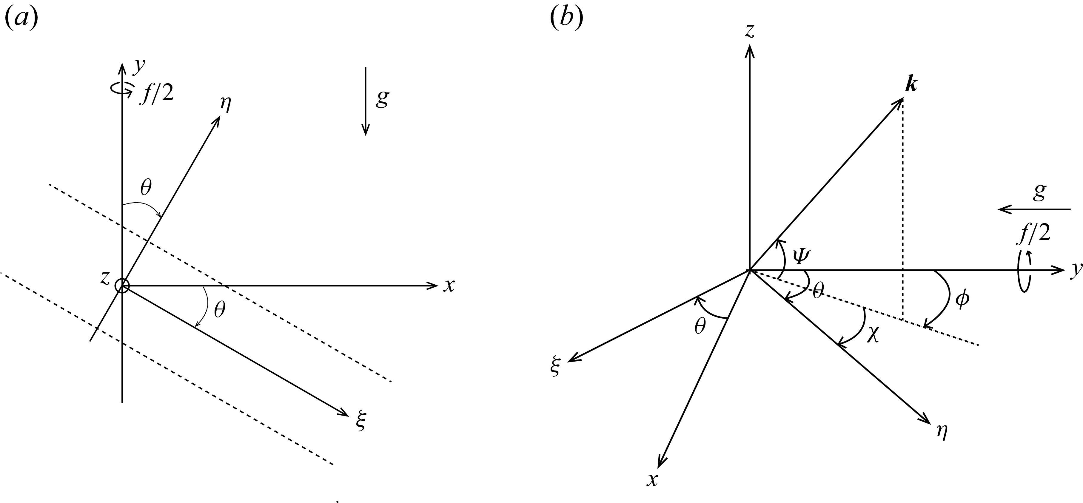
 ω
 θ
 η
 χ
 ψ
 k=q
 t=0
 (α,β,γ)
 k
 χ
 ψ
 ϕ=θ−χ

 λr
 κ=ϵk
 ψ
 ϵ=0.01
 ϵ=0.1
 ψ=0
 κ≫1
 f=0
 ω=0.8
 ψ=π/20
 ψ=π/10
 ω=2.5
 f=10
 ψ=π/6
 ψ=π/3
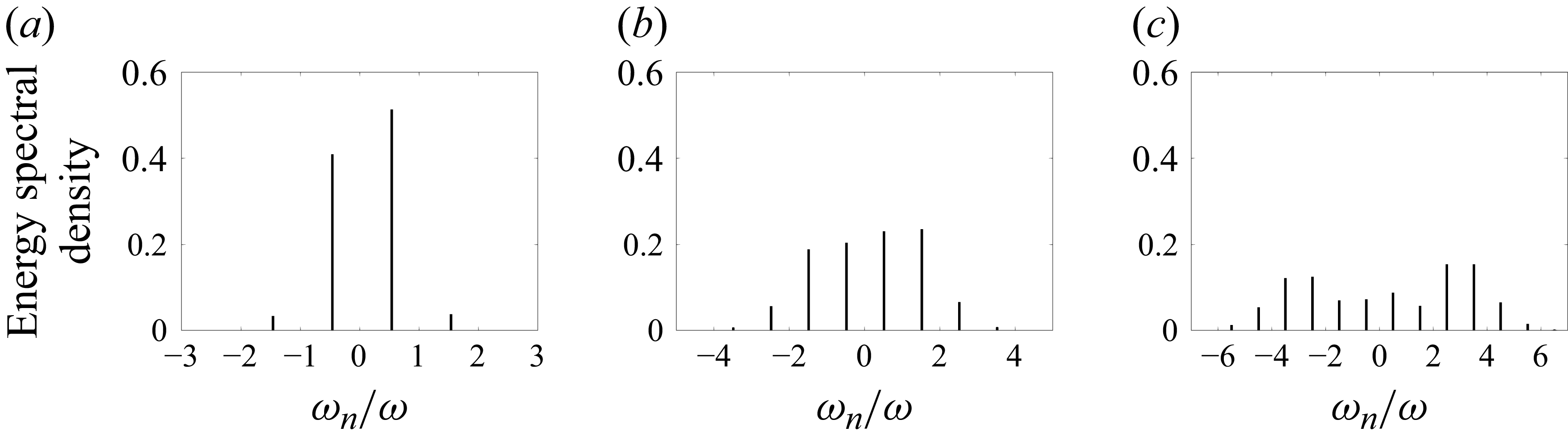
 κ=ϵk
 ω=2.5
 ϵ=0.1
 f=10
 ψ=π/3
 ωn=σr+nω
 n=0,±1,±2,…
 σ=σr+iσi
 κ=1.74
 κ=4.2
 κ=8.66


