1 Introduction
This paper is concerned with the question of how fluid inertia affects the settling of a particle under gravity in a fluid at rest. Understanding how particles settle in a fluid is of fundamental importance in many different scientific problems. An important example is sedimentation in suspensions of non-spherical particles. Homogeneous suspensions of settling spheroids are unstable to the formation of spatial patterns (Koch & Shaqfeh Reference Koch and Shaqfeh1989; Mackaplow & Shaqfeh Reference Mackaplow and Shaqfeh1998; Tornberg & Gustavsson Reference Tornberg and Gustavsson2006; Metzger, Butler & Guazzelli Reference Metzger, Butler and Guazzelli2007; Shin, Koch & Subramanian Reference Shin, Koch and Subramanian2009; Dahlklid Reference Dahlklid2011; Zhang et al. Reference Zhang, Dahlkild, Gustavsson and Lundell2014). The question is reviewed by Guazzelli & Hinch (Reference Guazzelli and Hinch2011). Other examples are plankton dynamics in the unsteady ocean (Jonsson Reference Jonsson1989; Guasto, Rusconi & Stocker Reference Guasto, Rusconi and Stocker2012; Gustavsson et al. Reference Gustavsson, Berglund, Jonsson and Mehlig2016), particle deposition (Charru, Mouilleron & Eiff Reference Charru, Mouilleron and Eiff2004) and the settling of ice particles in clouds, a process relevant for the onset and nature of precipitation (Pruppacher & Klett Reference Pruppacher and Klett2010).
When the particle is very small, the particle dynamics can be computed in the creeping-flow limit, assuming that inertial effects are negligible. For larger particles, when the particle Reynolds number is finite, then fluid inertia must be considered. It is known, for example, that weak fluid inertia causes a sphere to settle more slowly. This is a consequence of the disturbance flow created by the sphere at small particle Reynolds number. The corresponding disturbance problem (the ‘Oseen problem’) was solved by Proudman & Pearson (Reference Proudman and Pearson1957) using matched asymptotic expansions. Fluid inertia also affects the transient settling of a sphere, before the steady state is reached (Sano Reference Sano1981; Mei Reference Mei1992; Lovalenti & Brady Reference Lovalenti and Brady1993).
For non-spherical particles, less is known about the effects of fluid inertia. Only quite recently it was determined from first principles how weak fluid inertia modifies the torque on a spheroid in a simple shear (Subramanian & Koch Reference Subramanian and Koch2005; Candelier et al. Reference Candelier, Einarsson, Lundell, Mehlig and Angilella2015; Einarsson et al. Reference Einarsson, Candelier, Lundell, Angilella and Mehlig2015a ,Reference Einarsson, Candelier, Lundell, Angilella and Mehlig b ; Rosén et al. Reference Rosén, Einarsson, Nordmark, Aidun, Lundell and Mehlig2015).
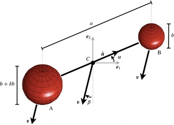
Illustration of the dumbbell and the notation used in this article. The centres of two spheres (A and B) of diameters
 $b+\unicode[STIX]{x1D6FF}b$
and
 $b$
are linked by a massless rigid rod of length
 $a$
. The centre of mass of the dumbbell is denoted by
 $C$
, and its velocity by
 $\boldsymbol{v}$
. The angle of the centre-of-mass velocity with the direction of gravity (negative
 $\boldsymbol{e}_{2}$
direction) is denoted by
 $\unicode[STIX]{x1D6FD}$
. As drawn, the angle is negative,
 $\unicode[STIX]{x1D6FD}<0$
. Since we consider a steady state where the angular velocity of the dumbbell vanishes (see text), the centre-of-mass velocities of both spheres are also
 $\boldsymbol{v}$
. The angle of inclination of the dumbbell (defined by the unit vector
 $\hat{\boldsymbol{n}}$
) with respect to the plane orthogonal to gravity (the
 $\boldsymbol{e}_{1}$
–
 $\boldsymbol{e}_{3}$
plane) is denoted by
 $\unicode[STIX]{x1D6FC}$
.

How does a non-spherical particle settle in a fluid at rest? Consider a small needle released at an inclination angle
 $\unicode[STIX]{x1D6FC}$
with the horizontal. If fluid inertia is negligible, then the needle continues to settle at this angle if it is fore–aft symmetric. Its centre of mass moves at an angle
 $\unicode[STIX]{x1D6FD}$
with the direction of gravity (figure 1). This angle is given by
 $$\begin{eqnarray}\tan \unicode[STIX]{x1D6FD}=\frac{\sin (2\unicode[STIX]{x1D6FC})}{\cos (2\unicode[STIX]{x1D6FC})-3}.\end{eqnarray}$$
Equation (1.1) is obtained in the creeping-flow limit for a slender body with fore–aft symmetry, as discussed by Happel & Brenner (Reference Happel and Brenner1983). See equation (5-11.33) in that book.
Khayat & Cox (Reference Khayat and Cox1989) analysed how weak fluid inertia affects the settling needle in the slender-body approximation. They found that a needle with fore–aft symmetry exhibits two equilibrium orientations: vertical (
 $\unicode[STIX]{x1D6FC}=\unicode[STIX]{x03C0}/2$
) and horizontal (
 $\unicode[STIX]{x1D6FC}=0$
). Only the horizontal equilibrium is stable. Khayat & Cox (Reference Khayat and Cox1989) concluded that the needle turns as it falls until it reaches horizontal orientation,
 $\unicode[STIX]{x1D6FC}=0$
, and then it continues to fall horizontally. This implies that its centre-of-mass velocity is aligned with the direction of gravity, that is,
 $\unicode[STIX]{x1D6FD}=0$
.
Dabade, Navaneeth & Subramanian (Reference Dabade, Navaneeth and Subramanian2015) computed how weak fluid inertia affects the orientation at which spheroids with arbitrary aspect ratios settle in a quiescent fluid. They found that, when settling in a fluid at rest, weak fluid inertia causes an oblate spheroid to align its axis of rotational symmetry with the direction of gravity.
Now consider a slender body that is rotationally symmetric but does not possess fore–aft symmetry. In the creeping-flow limit one expects the body to turn as it settles until it is oriented vertically (
 $\unicode[STIX]{x1D6FC}=\unicode[STIX]{x03C0}/2$
). But fluid inertia exerts a torque that tends to turn the body towards the horizontal. As mentioned by Khayat & Cox (Reference Khayat and Cox1989) this may cause the slender body to fall at an equilibrium angle that depends upon the degree of asymmetry of the body. In this paper we calculate this angle for a dumbbell without fore–aft symmetry. We use the method of reflection (Kim & Karrila Reference Kim and Karrila1991) to calculate the torque on the dumbbell, taking into account convective fluid inertia to linear order in the Reynolds number
 $\mathit{Re}_{b}=bv/\unicode[STIX]{x1D708}$
. Here
 $b$
is the diameter of the needle,
 $v$
is its centre-of-mass velocity and
 $\unicode[STIX]{x1D708}$
is the kinematic viscosity of the fluid.
To conclude § 1, we briefly comment on the wider context of this work. More generally, the settling of particles in turbulent flows is of interest. Maxey (Reference Maxey1987) showed that turbulence can enhance the settling speed of spherical particles. Recent experimental and numerical results on the settling of spherical particles in turbulence are discussed by Good et al. (Reference Good, Ireland, Bewley, Bodenschatz, Collins and Warhaft2014). The dynamics of neutrally buoyant non-spherical particles in turbulence has been investigated by a number of authors (Gustavsson, Einarsson & Mehlig Reference Gustavsson, Einarsson and Mehlig2014; Parsa & Voth Reference Parsa and Voth2014; Byron et al. Reference Byron, Einarsson, Gustavsson, Voth, Mehlig and Variano2015; Soldati & Voth Reference Soldati and Voth2017), but little is known about the settling of heavy non-spherical particles in turbulence.
2 Formulation of the problem
We consider a simple model system: a dumbbell composed of two spheres, A and B. Their centres are linked by a massless rigid rod of length
 $a$
(figure 1). Both spheres have the same mass density
 $\unicode[STIX]{x1D70C}_{p}$
, so that the centre of mass of the dumbbell coincides with its geometrical centre. This means that the dumbbell experiences no gravitational torque with respect to its geometrical centre. But we mention that the effect of gravitational torques on particles with inhomogeneous mass densities (‘gyrotaxis’) is important for the motion of certain plankton species (Durham et al.
Reference Durham, Climent, Barry, de Lillo, Boffetta, Cencini and Stocker2013; Zhan et al.
Reference Zhan, Sardina, Lushi and Brandt2014).
Sphere A has diameter
 $b+\unicode[STIX]{x1D6FF}b$
. Sphere B has diameter
 $b$
. We take
 $\unicode[STIX]{x1D6FF}b>0$
and define two dimensionless parameters that characterise the shape of the dumbbell:
 $$\begin{eqnarray}\unicode[STIX]{x1D706}\equiv \frac{\unicode[STIX]{x1D6FF}b}{b}\geqslant 0\quad \text{and}\quad \unicode[STIX]{x1D705}\equiv \frac{a}{b}.\end{eqnarray}$$
Here
 $\unicode[STIX]{x1D706}$
measures of the asymmetry of the dumbbell and
 $\unicode[STIX]{x1D705}$
defines its aspect ratio. We note that Khayat & Cox (Reference Khayat and Cox1989) define their parameter
 $\unicode[STIX]{x1D705}$
differently. In the following it is assumed that the dumbbell is slender and that its asymmetry is small:
 $$\begin{eqnarray}\unicode[STIX]{x1D705}\gg 1\quad \text{and}\quad \unicode[STIX]{x1D706}\ll 1.\end{eqnarray}$$
We do not consider the transient dynamics of the dumbbell but analyse its steady-state dynamics where the angular velocity of the dumbbell vanishes:
 $$\begin{eqnarray}\unicode[STIX]{x1D74E}=\mathbf{0}.\end{eqnarray}$$
In this case the two spheres settle with the same constant velocity
 $\boldsymbol{v}$
. We write
 $$\begin{eqnarray}\boldsymbol{v}=v\sin \unicode[STIX]{x1D6FD}\boldsymbol{e}_{1}-v\cos \unicode[STIX]{x1D6FD}\boldsymbol{e}_{2}.\end{eqnarray}$$
Here
 $\unicode[STIX]{x1D6FD}$
is the angle between the velocity vector and the direction of gravity (the negative
 $\boldsymbol{e}_{2}$
direction, figure 1), and
 $v$
is the magnitude of this velocity. To completely determine the steady-state dynamics of the dumbbell, it remains to specify its angle of inclination
 $\unicode[STIX]{x1D6FC}$
with the plane orthogonal to gravity (figure 1). We write
 $$\begin{eqnarray}\hat{\boldsymbol{n}}=\cos (\unicode[STIX]{x1D6FC})\boldsymbol{e}_{1}+\sin (\unicode[STIX]{x1D6FC})\boldsymbol{e}_{2}.\end{eqnarray}$$
The three unknowns of the problem (
 $v$
,
 $\unicode[STIX]{x1D6FC}$
and
 $\unicode[STIX]{x1D6FD}$
) are determined by three equations that are derived from the steady-state condition, namely that the force on the dumbbell and the torque with respect to its centre of mass
 $C$
must vanish in the steady state. The force condition reads
 $$\begin{eqnarray}\displaystyle \mathbf{0} & = & \displaystyle \boldsymbol{f}_{A}+\boldsymbol{f}_{B}.\end{eqnarray}$$
Here
 $\boldsymbol{f}_{A}$
and
 $\boldsymbol{f}_{B}$
are the forces acting on spheres A and B, and
 $\boldsymbol{x}_{A}$
and
 $\boldsymbol{x}_{B}$
are the position vectors of their centres. The torque condition
 $$\begin{eqnarray}\displaystyle & \displaystyle \mathbf{0}=\unicode[STIX]{x1D749}_{A}+(\boldsymbol{x}_{A}-\boldsymbol{x}_{C})\times \boldsymbol{f}_{A}+\unicode[STIX]{x1D749}_{B}+(\boldsymbol{x}_{B}-\boldsymbol{x}_{C})\times \boldsymbol{f}_{B} & \displaystyle\end{eqnarray}$$
is the sum of the hydrodynamic torques centred on the spheres,
 $\unicode[STIX]{x1D749}_{A}$
and
 $\unicode[STIX]{x1D749}_{B}$
, and the torques with respect to the centre of mass
 $\boldsymbol{x}_{C}$
of the dumbbell. Equations (2.6) and (2.7) provide three independent conditions because the forces lie in the plane spanned by
 $\boldsymbol{e}_{1}$
and
 $\boldsymbol{e}_{2}$
. The first equation gives two conditions, the second just one. It turns out that the torques
 $\unicode[STIX]{x1D749}_{A}$
and
 $\unicode[STIX]{x1D749}_{B}$
are negligible (§ 3). In this case it follows from (2.6) and (2.7) that the forces
 $\boldsymbol{f}_{A}$
and
 $\boldsymbol{f}_{B}$
must align with the vector
 $\boldsymbol{x}_{A}-\boldsymbol{x}_{B}$
.
The spheres are subject to gravity and to the forces exerted by the fluid. The main difficulty lies in determining the force exerted by the fluid on each sphere. To this end, we must solve the Navier–Stokes equations governing the fluid velocity and pressure. We note that the partial time derivative of the fluid velocity evaluates to zero in the frame translating with the centre of mass of the particle, since the dumbbell is assumed to settle with a time-independent velocity. In this frame of reference the Navier–Stokes equations read
 $$\begin{eqnarray}\unicode[STIX]{x1D735}\boldsymbol{\cdot }\boldsymbol{u}=0,\quad \unicode[STIX]{x1D70C}_{f}(\boldsymbol{u}\boldsymbol{\cdot }\unicode[STIX]{x1D735})\boldsymbol{u}=-\unicode[STIX]{x1D735}p+\unicode[STIX]{x1D707}\unicode[STIX]{x0394}\boldsymbol{u}+\unicode[STIX]{x1D70C}_{f}\boldsymbol{g}.\end{eqnarray}$$
The boundary conditions read
 $$\begin{eqnarray}\boldsymbol{u}=\mathbf{0}\quad \text{for}~\boldsymbol{x}\in \mathscr{S}=\mathscr{S}_{A}\cup \mathscr{S}_{B}\quad \text{and}\quad \boldsymbol{u}\rightarrow -\boldsymbol{v}\quad \text{as}~|\boldsymbol{x}|\rightarrow \infty .\end{eqnarray}$$
Here
 $\boldsymbol{u}$
is the fluid velocity as seen by the particle,
 $\unicode[STIX]{x1D707}=\unicode[STIX]{x1D70C}_{f}\unicode[STIX]{x1D708}$
is the dynamic viscosity of the fluid,
 $\unicode[STIX]{x1D708}$
is the kinematic viscosity,
 $\unicode[STIX]{x1D70C}_{f}$
is its density,
 $p$
is pressure,
 $\boldsymbol{g}$
is the gravitational acceleration pointing in the
 $-\boldsymbol{e}_{2}$
direction, and
 $\mathscr{S}_{A}$
and
 $\mathscr{S}_{B}$
are the surfaces of the spheres A and B. We follow Maxey & Riley (Reference Maxey and Riley1983) and decompose the fluid velocity and pressure as follows:
 $$\begin{eqnarray}\boldsymbol{u}=-\boldsymbol{v}+\boldsymbol{u}^{1}\quad \text{and}\quad p=(\unicode[STIX]{x1D70C}_{f}\,\boldsymbol{g}\boldsymbol{\cdot }\boldsymbol{x}+p_{\infty })+p^{1}.\end{eqnarray}$$
Here
 $-\boldsymbol{v}$
is the undisturbed fluid velocity in the frame translating with the centre of mass of the particle,
 $\unicode[STIX]{x1D70C}_{f}\,\boldsymbol{g}\boldsymbol{\cdot }\boldsymbol{x}+p_{\infty }$
is the (undisturbed) hydrostatic pressure, and
 $\boldsymbol{u}^{1}$
and
 $p^{1}$
are corrections to the fluid velocity and pressure due to the disturbance caused by the dumbbell.
The forces
 $\boldsymbol{f}_{A}$
and
 $\boldsymbol{f}_{B}$
are given by
 $$\begin{eqnarray}\boldsymbol{f}_{A}=(m_{A}-m_{fA})\boldsymbol{g}+\int _{\mathscr{S}_{A}}\unicode[STIX]{x1D748}^{1}\,\text{d}\boldsymbol{s}\quad \text{and}\quad \boldsymbol{f}_{B}=(m_{B}-m_{fB})\boldsymbol{g}+\int _{\mathscr{S}_{B}}\unicode[STIX]{x1D748}^{1}\,\text{d}\boldsymbol{s}.\end{eqnarray}$$
The terms proportional to
 $\boldsymbol{g}$
are forces due to the undisturbed pressure (Archimedean forces) and gravitational forces. Here
 $m_{A}$
and
 $m_{B}$
are the masses of the spheres, and
 $m_{fA}$
and
 $m_{fB}$
are the equivalent fluid masses. The remaining terms in (2.11) are forces due to the disturbance. They are integrals over the fluid stress tensor
 $\unicode[STIX]{x1D748}^{1}=-p^{1}\unicode[STIX]{x1D644}+2\unicode[STIX]{x1D707}\unicode[STIX]{x1D64E}^{1}$
of the disturbance. Here
 $\unicode[STIX]{x1D64E}^{1}$
is the symmetric part of the matrix of gradients of the disturbance flow velocity
 $\boldsymbol{u}^{1}$
. The integrals are over the surfaces
 $\mathscr{S}_{A}$
and
 $\mathscr{S}_{B}$
of the spheres, and
 $\text{d}\boldsymbol{s}$
is the surface element defined by the outward unit normal. The torques
 $\unicode[STIX]{x1D749}_{A}$
and
 $\unicode[STIX]{x1D749}_{B}$
are given by
 $$\begin{eqnarray}\unicode[STIX]{x1D749}_{A}=\int _{\mathscr{S}_{A}}(\boldsymbol{x}-\boldsymbol{x}_{A})\times \unicode[STIX]{x1D748}^{1}\,\text{d}\boldsymbol{s}\quad \text{and}\quad \unicode[STIX]{x1D749}_{B}=\int _{\mathscr{S}_{B}}(\boldsymbol{x}-\boldsymbol{x}_{B})\times \unicode[STIX]{x1D748}^{1}\,\text{d}\boldsymbol{s}.\end{eqnarray}$$
To determine
 $\unicode[STIX]{x1D748}^{1}$
, the disturbance problem must be solved. In the steady case the disturbance velocity
 $\boldsymbol{u}^{1}$
must satisfy
 $$\begin{eqnarray}\unicode[STIX]{x1D735}\boldsymbol{\cdot }\boldsymbol{u}^{1}=0,\quad \unicode[STIX]{x1D70C}_{f}[(\boldsymbol{u}^{1}-\boldsymbol{v})\boldsymbol{\cdot }\unicode[STIX]{x1D735}]\boldsymbol{u}^{1}=-\unicode[STIX]{x1D735}p^{1}+\unicode[STIX]{x1D707}\unicode[STIX]{x0394}\boldsymbol{u}^{1},\end{eqnarray}$$
with boundary conditions
 $$\begin{eqnarray}\boldsymbol{u}^{1}=\boldsymbol{v}\quad \text{for}~\boldsymbol{x}\in \mathscr{S}\quad \text{and}\quad \boldsymbol{u}^{1}\rightarrow \mathbf{0}\quad \text{as}~|\boldsymbol{x}|\rightarrow \infty .\end{eqnarray}$$
Equations (2.6), (2.7) and (2.11)–(2.14) constitute the problem to be solved.
3 Creeping-flow limit – method of reflection
In order to determine the forces due to the disturbance flow, we must determine
 $\unicode[STIX]{x1D748}^{1}$
by solving (2.13) with the boundary conditions (2.14).
Consider how the magnitude of the convective terms on the left-hand side of (2.13) compares to the magnitude of the viscous terms on the right-hand side of the same equation, in the vicinity of each sphere. It follows from the boundary condition (2.14) that the disturbance velocity
 $\boldsymbol{u}^{1}$
is of order
 $v$
. The length scale is given by
 $b$
. This allows us to estimate:
 $$\begin{eqnarray}\frac{\unicode[STIX]{x1D70C}_{f}(\boldsymbol{u}^{1}\boldsymbol{\cdot }\unicode[STIX]{x1D735})\boldsymbol{u}^{1}}{\unicode[STIX]{x1D707}\unicode[STIX]{x0394}\boldsymbol{u}^{1}}\sim \frac{\unicode[STIX]{x1D70C}_{f}(\boldsymbol{v}\boldsymbol{\cdot }\unicode[STIX]{x1D735})\boldsymbol{u}^{1}}{\unicode[STIX]{x1D707}\unicode[STIX]{x0394}\boldsymbol{u}^{1}}\sim O(\mathit{Re}_{b}).\end{eqnarray}$$
In the creeping-flow limit,
 $\mathit{Re}_{b}=0$
, these terms are negligible, so that (2.13) becomes the steady Stokes equation determining the hydrodynamic interactions between the two spheres. We compute these interactions using the method of reflection (Kim & Karrila Reference Kim and Karrila1991). The method of reflection is applied iteratively. First the sphere A is considered as if this sphere was alone in a fluid at rest. The disturbance flow at
 $\boldsymbol{x}$
can then be written as
 $$\begin{eqnarray}\boldsymbol{u}_{A}^{1(1)}(\boldsymbol{x})=-\left(1+\frac{b^{2}(1+\unicode[STIX]{x1D706})^{2}}{24}\,\unicode[STIX]{x0394}\right)\unicode[STIX]{x1D642}(\boldsymbol{x}-\boldsymbol{x}_{A})\boldsymbol{\cdot }\boldsymbol{f}_{A}^{1(1)}\end{eqnarray}$$
(the superscript in parentheses denotes the number of the iteration). The first term is the elementary solution of Stokes equation with a point force (stokeslet). The second term is a short-range correction due to the finite size of the particle. Moreover,
 $$\begin{eqnarray}\boldsymbol{f}_{A}^{1(1)}=-3\unicode[STIX]{x03C0}\unicode[STIX]{x1D707}b(1+\unicode[STIX]{x1D706})\boldsymbol{v}\end{eqnarray}$$
is the Stokes drag experienced by sphere A,
 $\boldsymbol{x}_{A}$
is its position and
 $\unicode[STIX]{x1D642}(\boldsymbol{y})$
is the Green tensor of the Stokes equation:
 $$\begin{eqnarray}\unicode[STIX]{x1D60E}_{ij}(\boldsymbol{y})=\frac{1}{8\unicode[STIX]{x03C0}\unicode[STIX]{x1D707}}\left(\frac{\unicode[STIX]{x1D6FF}_{ij}}{r}+\frac{y_{i}y_{j}}{r^{3}}\right),\quad r=|\boldsymbol{y}|.\end{eqnarray}$$
The minus sign in (3.2) arises from the fact that the sphere is seen by the fluid as a point force, with intensity equal to the Stokes drag experienced by the sphere, but with the opposite sign. The terms in (3.2) that account for the finite size of the particle are of order
 $(1+\unicode[STIX]{x1D706})^{3}b^{3}v/r^{3}$
. These terms thus contribute to the force acting on the sphere B at order
 $\unicode[STIX]{x1D705}^{-3}$
, at higher order than considered in our calculation. In the following we neglect these terms.
Second, the sphere B is introduced into the flow field
 $\boldsymbol{u}_{A}^{1(1)}$
, disregarding its effect on sphere A. To determine the force acting on sphere B, we use the first Faxén law (see e.g. Happel & Brenner Reference Happel and Brenner1983), which leads us to
 $$\begin{eqnarray}\boldsymbol{f}_{B}^{1(2)}\simeq -3\unicode[STIX]{x03C0}\unicode[STIX]{x1D707}b\left[\boldsymbol{v}-\boldsymbol{u}_{A}^{1(1)}(\boldsymbol{x}_{B})-\frac{b^{2}}{24}\unicode[STIX]{x0394}\boldsymbol{u}_{A}^{1(1)}(\boldsymbol{x}_{B})\right].\end{eqnarray}$$
The term involving the Laplacian is neglected in the following since it is of order
 $\unicode[STIX]{x1D705}^{-3}$
.
Third, consider the torque
 $\unicode[STIX]{x1D749}_{B}$
. In the creeping-flow limit, the torque centred on sphere B is given by
 $$\begin{eqnarray}\unicode[STIX]{x1D749}_{B}^{1(2)}\simeq \unicode[STIX]{x03C0}\unicode[STIX]{x1D707}b^{3}\unicode[STIX]{x1D734}_{f}(\boldsymbol{x}_{B})\quad \text{where}~\unicode[STIX]{x1D734}_{f}(\boldsymbol{x}_{B})={\textstyle \frac{1}{2}}\unicode[STIX]{x1D735}\times \boldsymbol{u}_{A}^{1(1)}(\boldsymbol{x}_{B}).\end{eqnarray}$$
Since
 $\unicode[STIX]{x1D734}_{f}(\boldsymbol{x}_{B})\sim bv/a^{2}$
, we see that this torque is smaller than the term
 $(\boldsymbol{x}_{B}-\boldsymbol{x}_{C})\times \boldsymbol{f}_{B}^{1(2)}$
by a factor of
 $\unicode[STIX]{x1D705}^{-3}$
.
Fourth, in the same way, the force and torque acting upon sphere A are computed. Taking the results together, we find to order
 $\unicode[STIX]{x1D705}^{-1}$
:
 $$\begin{eqnarray}\left.\begin{array}{@{}c@{}}\boldsymbol{f}_{A}=(m_{A}-m_{fA})\boldsymbol{g}-3\unicode[STIX]{x03C0}\unicode[STIX]{x1D707}b(1+\unicode[STIX]{x1D706})(\boldsymbol{v}-3\unicode[STIX]{x03C0}\unicode[STIX]{x1D707}b\unicode[STIX]{x1D642}(-\boldsymbol{a})\boldsymbol{\cdot }\boldsymbol{v})+O(\unicode[STIX]{x1D705}^{-2}),\\ \boldsymbol{f}_{B}=(m_{B}-m_{fB})\boldsymbol{g}-3\unicode[STIX]{x03C0}\unicode[STIX]{x1D707}b(\boldsymbol{v}-3\unicode[STIX]{x03C0}\unicode[STIX]{x1D707}b(1+\unicode[STIX]{x1D706})\unicode[STIX]{x1D642}(\boldsymbol{a})\boldsymbol{\cdot }\boldsymbol{v})+O(\unicode[STIX]{x1D705}^{-2}).\end{array}\right\}\end{eqnarray}$$
Here
 $\boldsymbol{a}=\boldsymbol{x}_{B}-\boldsymbol{x}_{A}$
. Inserting these expressions into (2.6) and (2.7) and noting that the torques
 $\unicode[STIX]{x1D749}_{A}$
and
 $\unicode[STIX]{x1D749}_{B}$
are negligible, we can determine
 $\unicode[STIX]{x1D6FC}$
,
 $v$
and
 $\unicode[STIX]{x1D6FD}$
in the creeping-flow limit.
3.1 Symmetric dumbbell
 $(\unicode[STIX]{x1D706}=0)$

For a symmetric dumbbell, the torque condition (2.7) is always satisfied in the creeping-flow limit. It follows that all inclination angles
 $\unicode[STIX]{x1D6FC}$
are steady-state solutions. This well-known result (Happel & Brenner Reference Happel and Brenner1983) means that the dumbbell continues to fall at its initial inclination. For a symmetric dumbbell, the force conditions (2.6) are readily solved to determine the centre-of-mass speed
 $v$
and the angle
 $\unicode[STIX]{x1D6FD}$
as functions of
 $\unicode[STIX]{x1D6FC}$
. We find
 $$\begin{eqnarray}\tan \unicode[STIX]{x1D6FD}=\frac{\sin (2\unicode[STIX]{x1D6FC})}{\cos (2\unicode[STIX]{x1D6FC})+3-\frac{16}{3}\unicode[STIX]{x1D705}}=-\frac{3\sin (2\unicode[STIX]{x1D6FC})}{16\unicode[STIX]{x1D705}}+O(\unicode[STIX]{x1D705}^{-2}).\end{eqnarray}$$
We have expanded (3.8) for large values of
 $\unicode[STIX]{x1D705}$
because our perturbative solution assumes that
 $\unicode[STIX]{x1D705}$
is large. In this limit the angular dependence in (3.8) is qualitatively similar to that in (1.1), derived for a thin needle with fore–aft symmetry (Happel & Brenner Reference Happel and Brenner1983). According to (3.8) the angle
 $\unicode[STIX]{x1D6FD}$
is negative for
 $0<\unicode[STIX]{x1D6FC}<\unicode[STIX]{x03C0}/2$
and it tends to zero as
 $\unicode[STIX]{x1D6FC}\rightarrow 0$
and
 $\unicode[STIX]{x1D6FC}\rightarrow \unicode[STIX]{x03C0}/2$
. An important difference between (1.1) and (3.8) is, however, that the angle
 $\unicode[STIX]{x1D6FD}$
is independent of the aspect ratio in the case of the needle, while it does depend on
 $\unicode[STIX]{x1D705}$
for the dumbbell. According to (3.8) the angle
 $\unicode[STIX]{x1D6FD}$
tends to zero in the limit
 $\unicode[STIX]{x1D705}\rightarrow \infty$
. This is simply a consequence of the fact that there are no hydrodynamic interactions between the spheres in this limit; they must fall as if they were independent, each at the same terminal velocity.
For the centre-of-mass speed we find
 $$\begin{eqnarray}v=\frac{m_{fB}(\unicode[STIX]{x1D6FE}-1)g}{3\unicode[STIX]{x03C0}b\unicode[STIX]{x1D707}}\left(1+\frac{6-3\cos (\unicode[STIX]{x1D6FC})^{2}}{8\unicode[STIX]{x1D705}}\right)+O(\unicode[STIX]{x1D705}^{-2}),\end{eqnarray}$$
where
 $\unicode[STIX]{x1D6FE}=m_{B}/m_{fB}$
. From (3.9) we infer that vertical orientation (
 $\unicode[STIX]{x1D6FC}=\unicode[STIX]{x03C0}/2$
) yields the fastest terminal velocity. We also see that, in general, the dumbbell settles faster than either sphere A or B alone. This is due to the disturbance flow.
3.2 Asymmetric dumbbell
$(\unicode[STIX]{x1D706}\neq 0)$

Now consider an asymmetric particle. When
 $\unicode[STIX]{x1D706}$
is not zero, then (2.6) and (2.7) admit the solutions
 $$\begin{eqnarray}\unicode[STIX]{x1D6FC}=\pm \unicode[STIX]{x03C0}/2,\quad \unicode[STIX]{x1D6FD}=0\end{eqnarray}$$
and
 $$\begin{eqnarray}v=\frac{m_{fB}(\unicode[STIX]{x1D6FE}-1)g}{3\unicode[STIX]{x03C0}\unicode[STIX]{x1D707}b}\left(1+\frac{3}{4\unicode[STIX]{x1D705}}+\unicode[STIX]{x1D706}\right)+O(\unicode[STIX]{x1D706}^{2},\unicode[STIX]{x1D705}^{-2},\unicode[STIX]{x1D706}\unicode[STIX]{x1D705}^{-1}).\end{eqnarray}$$
The asymmetric dumbbell settles vertically in the steady state. From the torque equation (2.7), it follows that
 $\unicode[STIX]{x1D6FC}=-\unicode[STIX]{x03C0}/2$
(the smaller sphere first) is unstable. By contrast,
 $\unicode[STIX]{x1D6FC}=\unicode[STIX]{x03C0}/2$
is stable. So when an asymmetric dumbbell is released in fluid at rest, then it tends to settle vertically, the larger sphere first.
4 Effect of fluid inertia
In this section we incorporate weak effects of fluid inertia on the dynamics of the dumbbell settling in a quiescent fluid, assuming that
 $\mathit{Re}_{b}$
is small but finite. As mentioned in § 1, Khayat & Cox (Reference Khayat and Cox1989) investigated the effect of fluid inertia on the settling of a needle with fore–aft symmetry (see also Dabade et al.
Reference Dabade, Navaneeth and Subramanian2015). What happens when fore–aft symmetry is broken? To answer this question, we need to determine the disturbance flow produced by a single sphere when convective inertia is taken into account. The disturbance flow produced by a single sphere corresponds, to leading order and in the vicinity of the sphere, to a Stokes flow plus a small correction. Since the Stokes solution scales as
 $vb/r$
, it follows that, far from the spheres, the convective term
 $\unicode[STIX]{x1D70C}_{f}(\boldsymbol{u}^{1}\boldsymbol{\cdot }\unicode[STIX]{x1D735})\boldsymbol{u}^{1}$
is always smaller than the viscous term
 $\unicode[STIX]{x1D707}\unicode[STIX]{x0394}\boldsymbol{u}^{1}$
and can be neglected. But the convective term
 $\unicode[STIX]{x1D70C}_{f}(\boldsymbol{v}\boldsymbol{\cdot }\unicode[STIX]{x1D735})\boldsymbol{u}^{1}$
decays more slowly than the viscous terms and must balance the viscous terms at a distance
 $b/\mathit{Re}_{b}$
, the Oseen length. At this distance, this convective term can no longer be neglected. In this way we are led to the Oseen equations.
4.1 Elementary solution of the Oseen equations
We use an iterative procedure, as in the previous section. The first step is to find an elementary closed-form solution of the Oseen equations. Keeping in mind that the two spheres are assumed to be far from each other (
 $\unicode[STIX]{x1D705}\gg 1$
), the rapidly decreasing terms with respect to
 $r$
in the solution of the Oseen equations can be neglected. We therefore consider the equations
 $$\begin{eqnarray}\unicode[STIX]{x1D735}\boldsymbol{\cdot }\boldsymbol{u}=0,\quad -\unicode[STIX]{x1D70C}_{f}(\boldsymbol{v}\boldsymbol{\cdot }\unicode[STIX]{x1D735})\boldsymbol{u}=-\unicode[STIX]{x1D735}p+\unicode[STIX]{x1D707}\unicode[STIX]{x0394}\boldsymbol{u}+\boldsymbol{f}\unicode[STIX]{x1D6FF},\end{eqnarray}$$
where the particle is represented by a point force (
 $\unicode[STIX]{x1D6FF}(\boldsymbol{x})$
stands for the Dirac delta function). The solution of (4.1) can be found in the literature (Pignatel, Nicolas & Guazzelli Reference Pignatel, Nicolas and Guazzelli2011), see also Happel & Brenner (Reference Happel and Brenner1983, p. 79). It can be obtained as follows. Applying the Fourier transform
 $$\begin{eqnarray}\boldsymbol{u}=\mathscr{F}\boldsymbol{u}\equiv \int _{\mathbb{R}^{3}}\boldsymbol{u}(\boldsymbol{y})\exp (-\text{i}\boldsymbol{k}\boldsymbol{\cdot }\boldsymbol{y})\,\text{d}\boldsymbol{y},\end{eqnarray}$$
to (4.1) we find
 $$\begin{eqnarray}\displaystyle & \displaystyle \boldsymbol{k}\boldsymbol{\cdot }\boldsymbol{u}=0,\quad -\text{i}\unicode[STIX]{x1D70C}_{f}(\boldsymbol{v}\boldsymbol{\cdot }\boldsymbol{k})\boldsymbol{u}=-\text{i}\boldsymbol{k}\tilde{p}-\unicode[STIX]{x1D707}k^{2}\boldsymbol{u}+\boldsymbol{f}. & \displaystyle\end{eqnarray}$$
As usual, the pressure is determined by projecting equation (4.3b
) along
 $\boldsymbol{k}$
. This yields
 $-\text{i}\tilde{p}=-\boldsymbol{f}\boldsymbol{\cdot }\boldsymbol{k}/k^{2}$
, and performing a partial fraction decomposition we are led to
 $$\begin{eqnarray}\boldsymbol{u}=\frac{\boldsymbol{f}}{(\unicode[STIX]{x1D707}\boldsymbol{k}-\text{i}\unicode[STIX]{x1D70C}_{f}\boldsymbol{v})\boldsymbol{\cdot }\boldsymbol{k}}-\left(\frac{\boldsymbol{f}\boldsymbol{\cdot }\boldsymbol{k}}{\unicode[STIX]{x1D70C}_{f}\boldsymbol{v}\boldsymbol{\cdot }\boldsymbol{k}}\right)\text{i}\boldsymbol{k}\left(\frac{1}{k^{2}}-\frac{\unicode[STIX]{x1D707}}{(\unicode[STIX]{x1D707}\boldsymbol{k}-\text{i}\unicode[STIX]{x1D70C}_{f}\boldsymbol{v})\boldsymbol{\cdot }\boldsymbol{k}}\right).\end{eqnarray}$$
This result simplifies: since the vectors
 $\boldsymbol{f}$
and
 $\boldsymbol{v}$
are collinear, we have
 $$\begin{eqnarray}\left(\frac{\boldsymbol{f}\boldsymbol{\cdot }\boldsymbol{k}}{\unicode[STIX]{x1D70C}_{f}\boldsymbol{v}\boldsymbol{\cdot }\boldsymbol{k}}\right)=\frac{f}{\unicode[STIX]{x1D70C}_{f}v},\end{eqnarray}$$
where
 $f=|\boldsymbol{f}|$
. Now we apply the inverse Fourier transform. Using the relations
 $$\begin{eqnarray}\mathscr{F}^{-1}\frac{1}{k^{2}}=\frac{1}{4\unicode[STIX]{x03C0}r}\quad \text{and}\quad \mathscr{F}^{-1}\frac{1}{(\unicode[STIX]{x1D707}\boldsymbol{k}-\text{i}\unicode[STIX]{x1D70C}_{f}\boldsymbol{v})\boldsymbol{\cdot }\boldsymbol{k}}=\frac{\text{exp}\left[-{\displaystyle \frac{1}{2\unicode[STIX]{x1D708}}}(vr+\boldsymbol{v}\boldsymbol{\cdot }\boldsymbol{y})\right]}{4\unicode[STIX]{x03C0}\unicode[STIX]{x1D707}r},\end{eqnarray}$$
we find
 $$\begin{eqnarray}\boldsymbol{u}=\frac{\text{exp}\left[-{\displaystyle \frac{1}{2\unicode[STIX]{x1D708}}}(vr+\boldsymbol{v}\boldsymbol{\cdot }\boldsymbol{y})\right]}{4\unicode[STIX]{x03C0}\unicode[STIX]{x1D707}r}\boldsymbol{f}-\frac{f}{\unicode[STIX]{x1D70C}_{f}v}\unicode[STIX]{x1D735}\frac{1-\text{exp}\left[-{\displaystyle \frac{1}{2\unicode[STIX]{x1D708}}}(vr+\boldsymbol{v}\boldsymbol{\cdot }\boldsymbol{y})\right]}{4\unicode[STIX]{x03C0}r}.\end{eqnarray}$$
Expanding the derivatives in (4.7) yields
 $$\begin{eqnarray}\displaystyle & \displaystyle \boldsymbol{u}=\frac{\text{exp}\left[-\displaystyle \frac{1}{2\unicode[STIX]{x1D708}}(vr+\boldsymbol{v}\boldsymbol{\cdot }\boldsymbol{y})\right]}{8\unicode[STIX]{x03C0}\unicode[STIX]{x1D707}r}\boldsymbol{f}+\left\{1-\left(1+\frac{vr}{2\unicode[STIX]{x1D708}}\right)\text{exp}\left[-\frac{1}{2\unicode[STIX]{x1D708}}(vr+\boldsymbol{v}\boldsymbol{\cdot }\boldsymbol{y})\right]\right\}\frac{f}{\unicode[STIX]{x1D70C}_{f}v}\frac{\boldsymbol{y}}{4\unicode[STIX]{x03C0}r^{3}}. & \displaystyle \nonumber\\ \displaystyle & & \displaystyle\end{eqnarray}$$
The next step is to apply the method of reflection, with (4.8) instead of (3.2).
4.2 Method of reflections
As a first step, the flow
 $\boldsymbol{u}_{A}^{1(1)}$
produced by the sphere A is considered as if it were alone in a fluid at rest. The result is given by (4.8) in which
 $\boldsymbol{f}$
is replaced by
 $3\unicode[STIX]{x03C0}b(1+\unicode[STIX]{x1D706})\boldsymbol{v}$
(that is, the Stokes drag, with a minus sign). The sphere B is then introduced into this flow. We note first that the flow produced by the sphere A is non-uniform. In the previous section we discussed the fact that Faxén corrections are negligible in our problem. One may ask whether the non-uniformity of
 $\boldsymbol{u}_{A}^{1(1)}$
may give rise to a Saffman lift force acting on the sphere B. It turns out that, in the equations governing the flow produced by the sphere B, effects of the convective terms due to the non-uniformity of
 $\boldsymbol{u}_{A}^{1(1)}$
are negligible compared to those arising from the Oseen convective terms of the form
 $\unicode[STIX]{x1D70C}_{f}\{[\boldsymbol{v}-\boldsymbol{u}_{A}^{1(1)}(\boldsymbol{x}_{B})]\boldsymbol{\cdot }\unicode[STIX]{x1D735}\}\boldsymbol{u}_{B}^{1(2)}$
. The lift force can therefore be neglected and the equations that govern the fluid velocity take the same form as (4.1) but where the velocity
 $\boldsymbol{v}$
has to be replaced by the relative velocity
 $\boldsymbol{v}-\boldsymbol{u}_{A}^{1(1)}(\boldsymbol{x}_{B})$
. The force acting on the sphere B (see e.g. Proudman & Pearson Reference Proudman and Pearson1957) is then given by
 $$\begin{eqnarray}\boldsymbol{f}_{B}^{1(2)}=-3\unicode[STIX]{x03C0}\unicode[STIX]{x1D707}b\left(1+{\textstyle \frac{3}{16}}\mathit{Re}_{b}\right)[\boldsymbol{v}-\boldsymbol{u}_{A}^{1(1)}(\boldsymbol{x}_{B})]+O(\unicode[STIX]{x1D705}^{-2},\unicode[STIX]{x1D706}\mathit{Re}_{b},\mathit{Re}_{b}\unicode[STIX]{x1D705}^{-1})\end{eqnarray}$$
(note that
 $\boldsymbol{u}_{A}^{1(1)}$
depends on
 $\mathit{Re}_{b}$
). Similarly, the disturbance force acting on the sphere A reads as
 $$\begin{eqnarray}\boldsymbol{f}_{A}^{1(2)}=-3\unicode[STIX]{x03C0}\unicode[STIX]{x1D707}b(1+\unicode[STIX]{x1D706})\left(1+{\textstyle \frac{3}{16}}\mathit{Re}_{b}\right)[\boldsymbol{v}-\boldsymbol{u}_{B}^{1(1)}(\boldsymbol{x}_{A})]+O(\unicode[STIX]{x1D705}^{-2},\unicode[STIX]{x1D706}\mathit{Re}_{b},\mathit{Re}_{b}\unicode[STIX]{x1D705}^{-1}).\end{eqnarray}$$
4.3 Results
Inserting the disturbance forces (4.9) and (4.10) into (2.11) and solving (2.6) and (2.7) yields the desired solution. In general, this must be done numerically. Here we consider the limit
 $\unicode[STIX]{x1D705}\mathit{Re}_{b}\ll 1$
. In this case we can obtain explicit expressions by expanding the Oseen solution (4.8). In this way we find that the angle of inclination tends to the equilibrium value
 $$\begin{eqnarray}\unicode[STIX]{x1D6FC}=\left\{\begin{array}{@{}ll@{}}\displaystyle \arcsin \left(\frac{16\unicode[STIX]{x1D706}}{3\mathit{Re}_{b}}\right)+O(\unicode[STIX]{x1D705}\unicode[STIX]{x1D706}) & \text{when}~\displaystyle \frac{16\unicode[STIX]{x1D706}}{3\mathit{Re}_{b}}<1,\\ \displaystyle \frac{\unicode[STIX]{x03C0}}{2} & \text{otherwise.}\end{array}\right.\end{eqnarray}$$
As expected, it follows from (4.11) that a sufficiently asymmetric dumbbell falls in vertical orientation. A perfectly symmetric dumbbell, by contrast, settles in the horizontal orientation, like a fore–aft symmetric slender body (Khayat & Cox Reference Khayat and Cox1989). This is a consequence of the fact that the Oseen solution breaks the symmetry of the Stokes solution. But when the effect of breaking fore–aft symmetry and of convective fluid inertia balance, then the dumbbell falls at the equilibrium inclination determined by (4.11). For
 $\mathit{Re}_{b}=0.1$
, for example, a slight asymmetry of 1 %,
 $\unicode[STIX]{x1D706}=0.01$
, causes the dumbbell to settle at an inclination angle different from zero. The vector
 $\hat{\boldsymbol{n}}$
forms an angle of roughly 30° with the horizontal according to (4.11), as schematically shown in figure 1. One expects slender particles to exhibit a qualitatively similar behaviour and this could be tested experimentally by observing a small rod settling in a quiescent fluid at small Reynolds number.
Equation (4.11) shows that the angle is independent of
 $\unicode[STIX]{x1D705}$
when
 $\unicode[STIX]{x1D705}\mathit{Re}_{b}$
small. This is a consequence of a property of the Oseen solution that is particular to the dumbbell. Expanding the Oseen solution assuming that
 $a$
is of the order of or smaller than
 $b/\mathit{Re}_{b}$
, we deduce that there is a uniform contribution to the fluid velocity that is proportional to
 $\mathit{Re}_{b}$
. This means that the inertial torque is proportional to
 $a$
. Since the contribution to the torque from the particle asymmetry is also proportional to
 $a$
, it follows that
 $\unicode[STIX]{x1D6FC}$
is independent of
 $\unicode[STIX]{x1D705}$
. A slender body behaves slightly differently, since the torque has a different dependence upon
 $a$
. See (6.12) and (6.22) in Khayat & Cox (Reference Khayat and Cox1989). When
 $\unicode[STIX]{x1D705}\mathit{Re}_{b}\ll 1$
, the angular dependence of the inertial torque is the same for the dumbbell as for a thin needle, proportional to
 $\sin (2\unicode[STIX]{x1D6FC})$
.
At the order considered here, the angle
 $\unicode[STIX]{x1D6FD}$
of the centre-of-mass velocity is found to remain unchanged compared with the creeping-flow limit (3.8). The settling speed is given by
 $$\begin{eqnarray}v=\frac{m_{fB}(\unicode[STIX]{x1D6FE}-1)g}{3\unicode[STIX]{x03C0}b\unicode[STIX]{x1D707}}\left[\left(1+\frac{6-3\cos (\unicode[STIX]{x1D6FC})^{2}}{8\unicode[STIX]{x1D705}}\right)+\unicode[STIX]{x1D706}-\frac{3}{8}\mathit{Re}_{b}\right]+O(\unicode[STIX]{x1D716}^{2}).\end{eqnarray}$$
Here
 $\unicode[STIX]{x1D716}^{2}$
denotes any quadratic combination of the small parameters
 $\unicode[STIX]{x1D705}^{-1}$
,
 $\unicode[STIX]{x1D706}$
or
 $\mathit{Re}_{b}$
. Equation (4.12) is consistent with the results obtained in the creeping-flow limit in § 3. In the limit
 $\mathit{Re}_{b}\rightarrow 0$
, (4.12) reduces to (3.9) for
 $\unicode[STIX]{x1D6FC}\neq 0$
,
 $\unicode[STIX]{x1D706}=0$
, and to (3.11) for
 $\unicode[STIX]{x1D6FC}=\unicode[STIX]{x03C0}/2$
,
 $\unicode[STIX]{x1D706}\neq 0$
.
5 Conclusions
We computed the hydrodynamic torque on an asymmetric dumbbell settling in a quiescent fluid, assuming that the Reynolds number
 $\mathit{Re}_{b}$
is small but finite. The two spheres have the same mass densities but different sizes. This asymmetry gives rise to an additional contribution to the torque that may balance the contribution of convective fluid inertia. In this case the dumbbell settles at an equilibrium angle that is determined by this balance. This prediction is expected to qualitatively hold more generally for particles of other shapes with broken fore–aft symmetry. When
 $\unicode[STIX]{x1D705}\mathit{Re}_{b}$
is small, the equilibrium angle of the settling dumbbell is independent of the value of the aspect ratio
 $\unicode[STIX]{x1D705}$
. This property is particular to the dumbbell; it does not hold for more general bodies.
In an independent study, Roy et al. (Reference Roy, Tierney, Voth and Koch2016) have analysed the settling of small rod-like and ramified particles without fore–aft symmetry that settle in a quiescent fluid, using slender-body approximations and experiments. It will be of interest for future work to determine the full range of particle shapes and flow parameters at which fore–aft asymmetry produces an equilibrium sedimentation angle that is neither horizontal nor vertical. It is of particular interest to answer the question: how robust are results derived assuming fore–aft symmetry?
Our results were obtained using the method of reflection. This method generates a perturbation expansion in the inverse of the aspect ratio
 $\unicode[STIX]{x1D705}$
of the dumbbell. The method makes it possible to systematically treat the dynamics of more general assemblies of spheres, partially linked. It allows, for instance, the computation of the dynamics of two dumbbells settling together, affecting each other but not coming too close to each other. The method used here is not restricted to quiescent flows. Applying the method of reflection for a neutrally buoyant symmetric dumbbell in a simple shear gives Jeffery’s equation (Jeffery Reference Jeffery1922), and it may be possible to treat the effect of fluid inertia upon the angular dynamics of the dumbbell using the method of § 4 and the reciprocal theorem (Subramanian & Koch Reference Subramanian and Koch2005; Einarsson et al.
Reference Einarsson, Candelier, Lundell, Angilella and Mehlig2015a
,Reference Einarsson, Candelier, Lundell, Angilella and Mehlig
b
).
Acknowledgements
This work was supported by grants from Vetenskapsrådet (grant no. 2013-3992), Formas (grant no. 2014-585), and by the grant ‘Bottlenecks for particle growth in turbulent aerosols’ from the Knut and Alice Wallenberg Foundation, Dnr. KAW 2014.0048.