1. Introduction
Natural convection associated with
 $\text{CO}_{2}$
sequestration in deep saline aquifers occurs due to the unstable density stratification of diffusive boundary layers. The density-driven instability plays a key role in the rapid dissolution of
 $\text{CO}_{2}$
into brine (Orr Reference Orr2009; Riaz & Cinar Reference Riaz and Cinar2014). We investigate the stability behaviour of gravitationally unstable, transient, diffusive boundary layers in the presence of permeability heterogeneity. The objective of this study is to develop a basic understanding of the instability mechanisms that govern the interaction of perturbations with permeability heterogeneity. We therefore take permeability to vary periodically across the thickness of the aquifer. Such a variation of permeability is relevant for saline aquifers (Chadwick, Arts & Eiken Reference Chadwick, Arts and Eiken2005; Bickle et al.
Reference Bickle, Chadwick, Huppert, Hallworth and Lyle2007; Neufeld & Huppert Reference Neufeld and Huppert2009; Green & Ennis-King Reference Green and Ennis-King2010) and also allows the identification of general mechanisms of instability in heterogeneous porous media.
A number of investigations of miscible flows in heterogeneous porous media highlight the importance of the interactions between fluid flow and permeability heterogeneity. These studies relate to displacement processes for oil recovery (Christie, Muggeridge & Barley Reference Christie, Muggeridge and Barley1993; Tchelepi et al. Reference Tchelepi, Orr, Rakotomalala, Salin and Woumeni1993; Zhang, Sorbie & Tsibuklis Reference Zhang, Sorbie and Tsibuklis1997), the flow of a contaminant jet into an aquifer (Schincariol, Schwartz & Mendoza Reference Schincariol, Schwartz and Mendoza1997; Schincariol Reference Schincariol1998) and the problem of natural convection due to a gravitationally unstable boundary layer (Simmons, Fenstemaker & Sharp Reference Simmons, Fenstemaker and Sharp2001; Prasad & Simmons Reference Prasad and Simmons2003; Rapaka et al. Reference Rapaka, Pawar, Stauffer, Zhang and Chen2009; Ranganathan et al. Reference Ranganathan, Farajzadeh, Bruining and Zitha2012). The presence of correlated variability of permeability leads to complex regimes. As the variance and the correlation length of permeability heterogeneity increase, the details of the permeability field dictate the flow paths (Tan & Homsy Reference Tan and Homsy1992; Tchelepi & Orr Reference Tchelepi and Orr1994; Chen & Meiburg Reference Chen and Meiburg1998; Camhi, Meiburg & Ruith Reference Camhi, Meiburg and Ruith2000). A resonant amplification of instability was reported by DeWit & Homsy (Reference DeWit and Homsy1997) and Riaz & Meiburg (Reference Riaz and Meiburg2004), which occurs when the length scale of the viscous instability is close to the correlation scale of the permeability variation.
The onset of natural convection depends on the growth rate of the perturbation amplitude within the linear regime. For the problem of
 $\text{CO}_{2}$
sequestration, the dynamic nature of the diffusive boundary layer imparts an evolutionary character to the growth of the amplitude that depends on the instantaneous coupling between the perturbations and the boundary layer. In the presence of heterogeneity, the coupling involves additional terms related to the permeability field, the effect of which has not been investigated for the onset of convection. In this study we characterize the onset of natural convection on the basis of the linear stability behaviour of diffusive boundary layers in heterogeneous porous media. Our approach is based on characterizing the mechanisms of vorticity production within the boundary layer. Among our main contributions is the identification of qualitatively different stability behaviours that depend upon the spatial scale of permeability variation relative to the instantaneous thickness of the boundary layer. Within a certain range of permeability phase, we find that the instability decreases with an increase in the variance if the permeability wavelength is small compared with the boundary layer thickness. The opposite effect of an increase in instability as a function of variance is observed in the limit of larger permeability wavelengths. We show that such behaviours are governed by two distinct modes of vorticity production that depend on the coupling between the fluctuations of permeability and concentration as well as the coupling between permeability gradients and velocity perturbations. Because of the unsteady nature of the diffusive boundary layer, the relative influence of these two modes changes in time. Consequently, we show that the evolutionary paths followed by the most amplified perturbations, up to the time for the onset of convection, are determined by the instantaneous competition between the two modes of vorticity production. The interpretation based on vorticity modes should also be useful for other problems. For example, McKibbin & O’Sullivan (Reference McKibbin and O’Sullivan1980) and Gjerde & Tyvand (Reference Gjerde and Tyvand1984) discuss the conditions under which localized convection may occur for the classical Rayleigh–Bénard convection in heterogeneous porous media. Though the classical Rayleigh–Bénard convection involves a steady basic state, in contrast to the current problem, the interaction of permeability with perturbation structures can be interpreted in a similar manner.
In order to carry out the stability analysis for transient boundary layers, we use initial perturbation profiles that are confined within the boundary layer (Riaz et al. Reference Riaz, Hesse, Tchelepi and Orr2006; Wessel-Berg Reference Wessel-Berg2009). We use statistical analysis to demonstrate that such profiles represent the most likely physical outcome from among all possible initial conditions. Our statistical results also indicate that the maximum instantaneous growth rate is bounded from above as time goes to zero, as predicted by the numerical abscissa of the linear operator (Trefethen & Embree Reference Trefethen and Embree2005). However, because of the uncertainty in the statistical ensemble, the upper bound is less likely to be observed in practice. More importantly though, Tilton, Daniel & Riaz (Reference Tilton, Daniel and Riaz2013) show that the perturbation profiles that maximize the instantaneous growth rate are not confined to the boundary layer and thus cannot lead to the onset of nonlinear convection in finite time. In order to determine the most amplified initial perturbation profile within the boundary layer, Daniel, Tilton & Riaz (Reference Daniel, Tilton and Riaz2013) employ an adjoint-based optimization analysis. These authors find that the dominant mode of Riaz et al. (Reference Riaz, Hesse, Tchelepi and Orr2006) is consistent with their optimal profile.
The paper is organized as follows. In § 2 we briefly describe the governing equations and the permeability model. In § 3 we compare the stability results based on perturbation profiles in the boundary layer with those obtained by conventional optimization methods. In § 4 we discuss the critical times for the onset of instability and describe a physical reasoning for the observed behaviour. In § 5 we consider the onset of convection and its connection to linear dynamics. Finally, a summary of our findings is presented in § 6.
2. Governing equations
The mathematical model governing the flow of dissolved
 $\text{CO}_{2}$
in a porous saline aquifer can be expressed in dimensionless form as
 $$\begin{eqnarray}\boldsymbol{{\rm\nabla}}\boldsymbol{\cdot }\boldsymbol{u}=0,\quad c_{t}=-\boldsymbol{u}\boldsymbol{\cdot }\boldsymbol{{\rm\nabla}}c+\frac{1}{\mathit{Ra}}{\rm\nabla}^{2}c,\quad \boldsymbol{u}=-k\left(\boldsymbol{{\rm\nabla}}p-c\hat{\boldsymbol{z}}\right),\end{eqnarray}$$
where
 $\boldsymbol{u}(\boldsymbol{x},t)$
is the Darcy velocity,
 $c(\boldsymbol{x},t)$
is the concentration,
 $p(\boldsymbol{x},t)$
the pressure. In (2.1),
 $\mathit{Ra}$
and
 $k(z)$
are dimensionless quantities corresponding to the Rayleigh number and permeability field. The unit vector,
 $\hat{\boldsymbol{z}}$
, acts in the direction of gravity,
 $g$
. The initial condition is the quiescent state,
 $\boldsymbol{u}=0$
. Periodic boundary conditions are imposed on the vertical boundaries. On the horizontal boundaries, we employ
 $$\begin{eqnarray}c|_{z=0}=1,\quad c_{z}|_{z=1}=0,\quad w|_{z=0}=w|_{z=1}=0.\end{eqnarray}$$
Equation (2.1) was non-dimensionalized as in Riaz et al. (Reference Riaz, Hesse, Tchelepi and Orr2006) with the following characteristic values for length, time, velocity, and pressure:
 $$\begin{eqnarray}L=H,\quad T=\frac{{\it\phi}{\it\mu}H}{\bar{k}{\rm\Delta}{\it\rho}g},\quad U=\frac{\bar{k}{\rm\Delta}{\it\rho}g}{{\it\mu}},\quad P=\frac{{\it\mu}UH}{\bar{k}},\end{eqnarray}$$
where
 $\bar{k}$
is a characteristic value of permeability,
 ${\it\phi}$
is the porosity, and
 $H$
the thickness of the aquifer. Concentration is scaled with respect to its maximum value found at
 $z=0$
. The Rayleigh number is defined as
 $\mathit{Ra}=UH/({\it\phi}D)$
, where
 $D$
is the diffusion coefficient. The driving mechanism of density difference is represented by
 ${\rm\Delta}{\it\rho}={\it\rho}_{1}-{\it\rho}_{o}$
, where
 ${\it\rho}_{o}$
and
 ${\it\rho}_{1}$
refer, respectively, to the density of pure brine and
 $\text{CO}_{2}$
saturated brine. The difference in density compared with the density of brine is small,
 ${\rm\Delta}{\it\rho}/{\it\rho}_{o}\sim {\rm\Delta}{\it\rho}/{\it\rho}_{1}\ll ~1$
(Yang & Gu Reference Yang and Gu2006; Nomeli, Tilton & Riaz Reference Nomeli, Tilton and Riaz2014). This justifies the use of the Boussinesq approximation and a linear density profile,
 ${\it\rho}={\it\rho}_{o}+{\rm\Delta}{\it\rho}c$
, for obtaining (2.1). The Boussinesq approximation further allows the velocity to be divergence free, as expressed in (2.1). Because contrasts in viscosity,
 ${\it\mu}$
, are relatively minor under typical aquifer conditions (Bando et al.
Reference Bando, Takemura, Nishio, Hihara and Akai2004; Fleury & Deschamps Reference Fleury and Deschamps2008), we will not consider them in the current analysis.
We take the dimensionless permeability field to vary periodically in the vertical direction according to
 $$\begin{eqnarray}k(z)=\exp \left[\sqrt{2{\it\sigma}^{2}}\cos (mz+{\it\gamma})\right].\end{eqnarray}$$
The term,
 $\sqrt{2{\it\sigma}^{2}}$
, indicates the amplitude of the spatial permeability oscillation, where
 ${\it\sigma}^{2}$
is the variance of
 $\ln (k)$
. The wavelength of permeability oscillation is
 $m$
, and
 ${\it\gamma}$
indicates the phase with respect to
 $z=0$
. The cosine permeability variation allows the spatial distribution to be smooth with a constant wavelength,
 $2{\rm\pi}/m$
. When
 $k(z)$
is normalized according to
 $\int _{0}^{1}k(z)\text{d}z=1$
, as in this work, then
 $\bar{k}$
corresponds to the average of the permeability field. The permeability model given by (2.4) includes the essential features of the spatial correlation of the permeability field and its variance (Freeze Reference Freeze1975; Delhomme Reference Delhomme1979). The variance associated with the spatial distribution of the natural logarithm of the permeability field has been reported to be within the range 0.5–5 (Clifton & Neuman Reference Clifton and Neuman1982), while the spatial correlation scales are often observed to be large horizontally and much smaller vertically (Dagan Reference Dagan1984), indicating a layered permeability structure. Porosity variation is not considered in this study because it is generally much less than the permeability variation (Hoeksema & Kitanidis Reference Hoeksema and Kitanidis1985).
3. Comparison of linear stability methods
We employ linear stability analysis for identifying the structure and growth of finite-amplitude perturbations that lead to the onset of nonlinear effects. Such perturbations are typically associated with the maximum eigenvalue of the linear operator when the base state is steady and the linear operator is normal. These conditions are not satisfied for the current problem. In the following, we evaluate the effectiveness of various methods in dealing with our problem by comparing with the statistical results of an initial value problem (IVP). To perform a linear stability analysis, we impose perturbations in the form of vertical shape functions that vary periodically in the
 $x$
and
 $y$
directions,
 $$\begin{eqnarray}(\boldsymbol{u},p,c)(\boldsymbol{x},t)=c^{o}(z,t)+(\tilde{\boldsymbol{u}},\tilde{p},\tilde{c})(z,t)\exp \left[\text{i}(\ell _{x}x+\ell _{y}y)\right],\end{eqnarray}$$
where
 $c^{o}$
is the concentration base state and
 $\tilde{\boldsymbol{u}},\tilde{p}$
and
 $\tilde{c}$
denote the perturbation profiles in the
 $z$
direction. Perturbation wavenumbers in the
 $x$
and
 $y$
direction are denoted by
 $\ell _{x}$
and
 $\ell _{y}$
, respectively, and
 $\text{i}=\sqrt{-1}$
.
The base state,
 $c^{o}(z,t)$
, is the solution of the diffusion equation,
 $c_{t}=c_{zz}/\mathit{Ra}$
, that follows from the initial condition,
 $\boldsymbol{u}=0$
, and the concentration boundary conditions, (2.2). This time-varying base state represents a diffusive boundary layer that originates at
 $z=0$
and diffuses downwards. By substituting (3.1) into (2.1), eliminating pressure and collecting linear terms, we obtain the following system for perturbations
 $\tilde{c}$
and
 $\tilde{w}$
:
 $$\begin{eqnarray}\displaystyle & \displaystyle \tilde{c}_{t}-\frac{1}{\mathit{Ra}}\left(\tilde{c}_{zz}-\ell ^{2}\tilde{c}\right)=-c_{z}^{o}\tilde{w}, & \displaystyle\end{eqnarray}$$
 $$\begin{eqnarray}\displaystyle & \tilde{w}_{zz}-(\ln k)_{z}\tilde{w}_{z}-\ell ^{2}\tilde{w}=-k\ell ^{2}\tilde{c}, & \displaystyle\end{eqnarray}$$
 $\ell =\sqrt{\ell _{x}^{2}+\ell _{y}^{2}}$
. The boundary conditions are
 $$\begin{eqnarray}\tilde{c}|_{z=0}=\tilde{c}_{z}|_{z=1}=\tilde{w}|_{z=0}=\tilde{w}|_{z=1}=0.\end{eqnarray}$$
The above set of equations represents a linear IVP with respect to the perturbations
 $\tilde{c}$
and
 $\tilde{w}$
. The IVP can be expressed more compactly as
 $$\begin{eqnarray}\frac{\partial \tilde{c}}{\partial t}={\mathcal{A}}(t;\ell )\tilde{c},\quad \tilde{c}(z,t_{o})=\tilde{c}_{o}(z);\quad z\in \{0,1\},\end{eqnarray}$$
where
 $t_{o}$
is the time at which perturbations are introduced, and
 ${\mathcal{A}}(t;\ell )$
is the linear operator that results from the elimination of
 $\tilde{w}$
between (3.2) and (3.3). The IVP can be marched in time to determine the evolution of the initial condition,
 $\tilde{c}_{o}(z)$
. The rate of instantaneous exponential growth associated with the evolution of
 $\tilde{c}_{o}(z)$
can be defined as
 $$\begin{eqnarray}{\it\omega}_{p}=\frac{\text{d}}{\text{d}t}\ln \Vert \tilde{c}(z,t)\Vert _{p},\end{eqnarray}$$
where
 $\Vert \cdot \Vert _{p}$
, indicates one of the
 $L^{\infty }$
,
 $L^{1}$
or
 $L^{2}$
norms that are defined, respectively, as
 $$\begin{eqnarray}\max _{z\in \{0,1\}}\{|\tilde{c}(z,t)|\},\quad \int _{0}^{1}|\tilde{c}(z,t)|\text{d}z\quad \text{and}\quad \left[\int _{0}^{1}\left(\tilde{c}(z,t)\right)^{2}\text{d}z\right]^{1/2}.\end{eqnarray}$$
The linear operator,
 ${\mathcal{A}}(t;\ell )$
, associated with the IVP, (3.5), is time varying and non-normal. For such problems, the maximum eigenvalue of
 $({\mathcal{A}}+{\mathcal{A}}^{\text{T}})/2$
can be interpreted as the maximum possible instantaneous growth rate,
 ${\it\omega}_{2}$
, that can be achieved by any initial condition as
 $t\rightarrow 0$
(Trefethen & Embree Reference Trefethen and Embree2005),
 $$\begin{eqnarray}\max \{{\it\lambda}(({\mathcal{A}}+{\mathcal{A}}^{\text{T}})/2)\}=\sup \{{\it\omega}_{2}:\tilde{c}_{o}(z)\in {\mathcal{R}}\},\end{eqnarray}$$
where
 ${\it\lambda}(({\mathcal{A}}+{\mathcal{A}}^{\text{T}})/2)$
refers to the eigenvalues of
 $({\mathcal{A}}+{\mathcal{A}}^{\text{T}})/2$
. The unsteady nature of the base state, however, makes the growth rate particularly sensitive to the initial condition,
 $\tilde{c}_{o}(z)$
. The effectiveness of this approach for the current problem is therefore unclear.
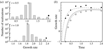
Figure 1(a) demonstrates the sensitivity to the initial condition, where we plot
 ${\it\omega}_{2}$
obtained from the IVP (3.5) based on a large number of initial conditions for
 $\mathit{Ra}=500$
,
 $\ell =8{\rm\pi}$
and
 ${\it\sigma}^{2}=0$
. Each realization of the initial condition is given by
 $\tilde{c}_{o}(z)={\it\Pi}r$
, where
 $r$
belongs to the set of random numbers distributed uniformly in
 $\{-1,1\}$
, and
 ${\it\Pi}$
is the box car function with a value of 1 for
 $0<z<z_{o}$
. In order to confine the initial perturbations inside the boundary layer, the location
 $z_{o}$
is selected to coincide with
 $c^{o}=10^{-2}$
. The histogram of the ensemble of
 ${\it\omega}_{2}$
, plotted at two different times in figure 1(a), shows that the distribution has a Gaussian-like character. Hence, the mean value (open circles) represents the most likely outcome of the ensemble, while the maximum value (filled circles) has a substantially lower probability. Figure 1(b) indicates that for small times the maximum value of the ensemble is bounded by the maximum eigenvalue of
 $({\mathcal{A}}+{\mathcal{A}}^{\text{T}})/2$
in accordance with (3.8). However, being far from the mean value of the ensemble, the maximum eigenvalue of
 $({\mathcal{A}}+{\mathcal{A}}^{\text{T}})/2$
is an imprecise estimate of the most likely statistical outcome.
(a) Histogram of the growth rate,
 ${\it\omega}_{2}$
, obtained from the IVP (3.5) based on
 $10^{4}$
realizations of initial conditions, at two different times, for
 $\mathit{Ra}=500$
,
 $\ell =8{\rm\pi}$
and
 ${\it\sigma}^{2}=0$
. (b) Comparison of IVP ensemble results, mean (open circles) and maximum (filled circles), with linear stability results based on the maximum eigenvalues of
 $({\mathcal{A}}+{\mathcal{A}}^{\text{T}})/2$
(dashed line) and
 ${\mathcal{B}}$
(dash-dotted line). The growth rate,
 ${\it\omega}_{2}$
, from IVP for
 $\tilde{c}_{o}=z{\it\alpha}\exp (-z^{2}{\it\alpha}^{2})$
(solid line) leads to good agreement with the ensemble mean.

The IVP (3.5) is also studied by considering a transformation of the underlying operator
 ${\mathcal{A}}$
. We employ the transformation
 ${\it\xi}=z{\it\alpha}$
and
 $\hat{t}=t$
, where
 ${\it\alpha}=\sqrt{\mathit{Ra }/4t}$
and
 ${\it\xi}\in \{0,\infty \}$
, to express (3.2) and (3.3) in
 $({\it\xi},t)$
-space, which gives the new IVP
 $$\begin{eqnarray}\frac{\partial \tilde{c}}{\partial t}={\mathcal{B}}(t;\ell )\tilde{c},\quad \tilde{c}({\it\xi},t_{o})=\tilde{c}_{o}({\it\xi});\quad {\it\xi}\in \{0,\infty \}.\end{eqnarray}$$
The base state in
 $({\it\xi},t)$
-space is self-similar,
 $c^{o}=\text{erfc}({\it\xi})$
, where erfc is the complementary error function. Homogeneous Dirichlet boundary conditions are employed for both
 $\tilde{c}$
and
 $\tilde{w}$
. The IVP in
 $({\it\xi},t)$
-space, (3.9), is equivalent to the IVP in
 $(z,t)$
-space, (3.5), provided
 ${\it\alpha}>3$
. When
 ${\it\alpha}>3$
, the two IVPs, (3.5) and (3.9), produce identical results when the growth rate for the IVP in self-similar space is transformed back to physical space according to
 $$\begin{eqnarray}\frac{\text{d}}{\text{d}t}\ln \Vert \tilde{c}(z,t)\Vert _{p}=\frac{\text{d}}{\text{d}t}\ln \Vert \tilde{c}({\it\xi},t)\Vert _{p}-f_{p}({\it\xi},t),\end{eqnarray}$$
with
 $$\begin{eqnarray}f_{\infty }=0,\quad f_{1}=\frac{1}{2t\Vert \tilde{c}({\it\xi},t)\Vert _{1}}\int _{0}^{\infty }{\it\xi}\frac{\partial |\tilde{c}|}{\partial {\it\xi}}\text{d}{\it\xi},\quad f_{2}=\frac{1}{2t\Vert \tilde{c}({\it\xi},t)\Vert _{2}^{2}}\int _{0}^{\infty }{\it\xi}\tilde{c}\frac{\partial \tilde{c}}{\partial {\it\xi}}\text{d}{\it\xi}.\end{eqnarray}$$
When
 ${\it\alpha}<3$
, the concentration profile interacts with the lower wall, in which case the solutions of (3.5) and (3.9) are no longer equivalent because of the different boundary conditions at
 $z=1$
.
Figure 1(b) demonstrates that the maximum eigenvalue of
 ${\mathcal{B}}$
(dash-dot line), transformed to the physical space with (3.10) based on the
 $L^{2}$
norm, is in close agreement with the mean value of the ensemble (open circles). Even though the operator,
 ${\mathcal{B}}$
, is time varying and non-normal, similar to
 ${\mathcal{A}}$
, the maximum eigenvalue of
 ${\mathcal{B}}$
is a good approximation of the ensemble mean. This is because the eigenfunctions of
 ${\mathcal{B}}$
are localized in the boundary layer (Ben, Demekhin & Chang Reference Ben, Demekhin and Chang2002; Riaz et al.
Reference Riaz, Hesse, Tchelepi and Orr2006), in contrast to either
 ${\mathcal{A}}$
or
 $({\mathcal{A}}+{\mathcal{A}}^{\text{T}})/2$
, and are thus better suited to represent the evolution of concentration perturbations originating within the boundary layer. Interestingly, we also find that the maximum eigenvalues of
 $({\mathcal{A}}+{\mathcal{A}}^{\text{T}})/2$
and
 $({\mathcal{B}}+{\mathcal{B}}^{\text{T}})/2$
are identical, i.e. the upper bound on the growth rate is independent of the coordinate transformation.
We next consider the initial profile suggested by Riaz et al. (Reference Riaz, Hesse, Tchelepi and Orr2006),
 $$\begin{eqnarray}\tilde{c}_{o}=z{\it\alpha}\exp (-z^{2}{\it\alpha}^{2}),\end{eqnarray}$$
which corresponds to the first eigenmode of the diffusion operator in self-similar space and is thus localized in the boundary layer. Figure 1(b) plots the growth rate,
 ${\it\omega}_{2}$
, obtained with an IVP using the initial condition, (3.12). The result (solid line) is in good agreement with the mean value of the ensemble. Tilton et al. (Reference Tilton, Daniel and Riaz2013) demonstrate that the onset of nonlinear convection occurs in finite time only for initial profiles, such as (3.12), that are localized within the boundary layer. Daniel et al. (Reference Daniel, Tilton and Riaz2013) show that the profile (3.12) coincides with the physically realizable optimal initial perturbations that maximize the amplification. Therefore, in this study, we use linear stability methods based on (3.12) and the eigenvalue problem based on the transformed operator,
 ${\mathcal{B}}$
, to characterize the linear instabilities.
4. Linear perturbation growth
We investigate the effect of permeability on the onset of linear instability. The onset of instability is defined as the time at which the perturbation growth rate first becomes positive,
 ${\it\omega}>0$
. The critical time for the onset of instability is defined as the minimum onset time of instability over all perturbation wavenumbers. A marginal state of stability corresponds to
 ${\it\omega}=0$
. To analyse the behaviour in the presence of heterogeneity, we consider the parameters of permeability variance,
 ${\it\sigma}^{2}$
, phase,
 ${\it\gamma}$
, permeability wavenumber,
 $m$
, in addition to perturbation wavenumber,
 $\ell$
, and time,
 $t$
. We perform our analysis for
 $\mathit{Ra}=500$
. Results for different
 $\mathit{Ra}$
are related through simple scaling relationships.
4.1. Influence of permeability variance and phase
The effect of permeability variance and phase on the marginal stability curve is shown in figure 2 for
 $\mathit{Ra}=500$
and
 $m=6{\rm\pi}$
. Two different values of the phase,
 ${\it\gamma}=0$
and
 ${\it\gamma}={\rm\pi}$
, are shown in plots (a) and (b), respectively. The marginal stability curve, for which
 ${\it\omega}=0$
, maps the boundaries of the stable (negative growth rate) and unstable (positive growth rate) regions in the
 $t{-}\ell$
plane. The lowest point on the curve, highlighted with a dot, indicates the critical conditions,
 $(t_{c},\ell _{c})$
, for the onset of instability, i.e. the earliest time,
 $t_{c}$
, at which the critical wavenumber,
 $\ell _{c}$
, becomes unstable. The critical time is greater than zero because perturbations are initially damped. The marginal stability curves also show the long-wave cutoff indicating that wavenumbers smaller than a critical value are damped.
Marginal stability curves for
 $\mathit{Ra}=500$
and
 $m=6{\rm\pi}$
, based on
 ${\it\omega}_{\infty }$
(lines) and
 ${\it\omega}_{DMA}$
(open symbols). (a)
 ${\it\gamma}=0$
and (b)
 ${\it\gamma}={\rm\pi}$
. Critical conditions for the onset of instability,
 $(t_{c},\ell _{c})$
, are indicated by solid dots. Increasing the variance for
 ${\it\gamma}=0$
results in greater instability, shifting the onset of instability to earlier times and larger wavenumbers. For the case of
 ${\it\gamma}={\rm\pi}$
, an increase in variance has the opposite effect.

The marginal stability curves based on the growth rate,
 ${\it\omega}_{\infty }$
, and the maximum eigenvalue of
 ${\mathcal{B}}$
are indicated with lines in figure 2. Symbols represent the growth rate,
 ${\it\omega}_{DMA}$
, obtained with the dominant mode analysis (DMA) of Riaz et al. (Reference Riaz, Hesse, Tchelepi and Orr2006), namely,
 $$\begin{eqnarray}{\it\omega}_{DMA}=-\frac{1}{4t}\left(4+{\it\beta}^{2}\right)+\frac{1}{a(t)\sqrt{{\rm\pi}t}}\int _{0}^{\infty }\exp (-{\it\xi}^{2})\tilde{w}\text{d}{\it\xi},\end{eqnarray}$$
where
 ${\it\beta}=\ell /{\it\alpha}$
,
 ${\it\alpha}=\sqrt{\mathit{Ra }/4t}$
and
 $a(t)$
is the coefficient in the expansion
 $\tilde{c}({\it\xi},t)=a(t){\it\xi}\text{e}^{-{\it\xi}^{2}}$
. For problems with homogeneous permeability, i.e.
 ${\it\sigma}^{2}=0$
, an analytical solution for
 $\tilde{w}$
can be used to obtain the following relation:
 $$\begin{eqnarray}{\it\omega}_{DMA}=-\frac{1}{4t}\left(4+{\it\beta}^{2}\right)+\frac{1}{16}\sqrt{\frac{{\rm\pi}}{t}}{\it\beta}^{2}\text{e}^{{\it\beta}^{2}/2}\left[1-\text{erf}\left(\frac{{\it\beta}}{2}\right)\right]^{2}.\end{eqnarray}$$
For heterogeneous cases, where
 ${\it\sigma}^{2}>0$
,
 $\tilde{w}$
can only be determined numerically. The integration in (4.1) is then carried out numerically to determine
 ${\it\omega}_{DMA}$
. The results based on
 ${\it\omega}_{DMA}$
are plotted to demonstrate the validity of DMA for the heterogeneous case. Figure 2(a) shows that the marginal stability curves based on
 ${\it\omega}_{DMA}$
and
 ${\it\omega}_{\infty }$
agree quite well for wavenumbers up to the critical wavenumber. Note that the time required for calculating critical conditions using DMA is at least an order of magnitude smaller than for other methods.
Figure 2(a) shows that when
 ${\it\gamma}=0$
, larger values of permeability variance,
 ${\it\sigma}^{2}$
, lead to greater instability (i.e. smaller critical times,
 $t_{c}$
), larger critical wavenumbers,
 $\ell _{c}$
, and a larger spectrum of unstable wavenumbers. Figure 2(b) indicates that the effect of variance is reversed when
 ${\it\gamma}={\rm\pi}$
. The critical time,
 $t_{c}$
, shifts to larger values with increasing variance while the critical wavenumber,
 $\ell _{c}$
, decreases, and the entire spectrum of unstable wavenumbers shrinks.
4.2. Stability mechanisms
A physical understanding of the effect of heterogeneity can be gained by considering the vorticity,
 $\boldsymbol{{\rm\nabla}}\times \boldsymbol{u}$
, which is obtained from (2.1) as
 $$\begin{eqnarray}\boldsymbol{{\rm\nabla}}\times \boldsymbol{u}=k\boldsymbol{{\rm\nabla}}c\times \hat{\boldsymbol{z}}+\boldsymbol{{\rm\nabla}}\ln k\times \boldsymbol{u}.\end{eqnarray}$$
The two terms on the right-hand side of (4.3) indicate that vorticity is produced or diminished by the interaction of two effects. The first term is related to the misalignment of the concentration gradient with the gravity vector,
 $\hat{\boldsymbol{z}}$
. The second term is associated with the misalignment of the velocity field with the gradient of
 $\ln k$
. For the homogeneous case,
 ${\it\sigma}^{2}=0$
, only the first term is present. For
 ${\it\sigma}^{2}>0$
, both terms contribute to either amplify or diminish vorticity. Note that the production of vorticity due to variable viscosity is given by
 $R\boldsymbol{{\rm\nabla}}c\times \boldsymbol{u}$
, where
 $R$
is the mobility ratio (Chen & Meiburg Reference Chen and Meiburg1998; Camhi et al.
Reference Camhi, Meiburg and Ruith2000; Riaz & Meiburg Reference Riaz and Meiburg2004; Daripa Reference Daripa2012; Daniel & Riaz Reference Daniel and Riaz2014). Although this term is similar to vorticity production by permeability gradients (4.3), the physical effect is different because of the transient nature of the concentration field as opposed to the fixed spatial variation of permeability.
To interpret vorticity in the linear regime for a two-dimensional disturbance field, we consider the
 $y$
-component of vorticity,
 ${\it\eta}(x,z,t)=\text{i}\tilde{{\it\eta}}(z,t)\,\exp (\text{i}\ell x)$
, which can be expressed as
 $$\begin{eqnarray}\tilde{{\it\eta}}=\ell k\tilde{c}-\frac{1}{\ell }(\ln k)^{\prime }\tilde{w}_{z}.\end{eqnarray}$$
The vorticity,
 $\tilde{{\it\eta}}$
, reflects the net effect of the coupling between perturbation and permeability profiles. The amplitude of perturbations,
 $\tilde{c}$
and
 $\tilde{w}$
, is governed by the history of perturbation growth. In order to focus on the effect of the instantaneous coupling between perturbation and permeability profiles, the concentration perturbation,
 $\tilde{c}$
, in (4.4) will be scaled with
 $\Vert \tilde{c}\Vert _{\infty }$
. The velocity perturbation,
 $\tilde{w}$
, then also scales with
 $\Vert \tilde{c}\Vert _{\infty }$
because the governing equations (3.2) and (3.3) are linear and do not contain the time derivative of
 $\tilde{w}$
. Note that the resulting instantaneous value of
 $\tilde{{\it\eta}}/\Vert \tilde{c}\Vert _{\infty }$
is useful for comparing the effect of different permeability profiles for a fixed value of
 $\ell$
. We also note that this approach is independent of the specific scale,
 $\Vert \tilde{c}\Vert _{p}$
, for
 $\tilde{c}$
and
 $\tilde{w}$
. Our interpretation and conclusions do not change when perturbations are scaled with either
 $\Vert \tilde{c}\Vert _{1}$
or
 $\Vert \tilde{c}\Vert _{2}$
.
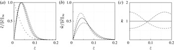
The spatial profiles for
 $\tilde{c}/\Vert \tilde{c}\Vert _{\infty }$
,
 $\tilde{w}/\Vert \tilde{c}\Vert _{\infty }$
and
 $k$
for
 $\mathit{Ra}=500$
, are plotted in figure 3 for
 $\ell =40$
,
 $m=6{\rm\pi}$
and
 $t=0.5$
. These perturbation profiles are based on the initial condition (3.12). The base state,
 $c^{o}$
, is also plotted in figure 3(a) to indicate that
 $\tilde{c}$
and
 $\tilde{w}$
decay rapidly to zero outside the boundary layer. Figure 3(a) shows that the profiles for
 $\tilde{c}/\Vert \tilde{c}\Vert _{\infty }$
do not change appreciably when heterogeneity is introduced. Therefore, the differences in the corresponding velocity perturbations,
 $\tilde{w}/\Vert \tilde{c}\Vert _{\infty }$
, plotted in figure 3(b), are mainly due to differences in the corresponding permeability profiles, shown in figure 3(c). Figure 3(b) shows that compared with the homogeneous case, the amplitude of
 $\tilde{w}/\Vert \tilde{c}\Vert _{\infty }$
increases for
 ${\it\gamma}=0$
but decreases when
 ${\it\gamma}={\rm\pi}$
. This behaviour can be understood with the help of (3.3). When
 $\tilde{c}$
and
 $\ell$
are fixed, larger positive values of
 $k(z)$
increase the magnitude of
 $\tilde{w}$
while larger negative values of
 $k(z)$
decrease the magnitude of
 $\tilde{w}$
.
Perturbation and permeability profiles for
 $\ell =40$
,
 $m=6{\rm\pi}$
and
 $t=0.5$
. Lines represent:
 ${\it\sigma}^{2}=0$
(solid),
 ${\it\sigma}^{2}=0.1,{\it\gamma}=0$
(dashed) and
 ${\it\sigma}^{2}=0.1,{\it\gamma}={\rm\pi}$
(dash-dotted). The base state,
 $c^{o}$
, is plotted in (a) with symbols. It indicates that perturbations rapidly decay to zero outside the boundary layer.

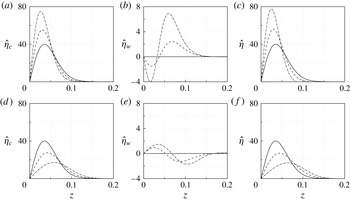
The perturbation–permeability interactions are shown in figure 4 with the help of
 $$\begin{eqnarray}\hat{{\it\eta}}_{c}=\ell k\tilde{c}/\Vert \tilde{c}\Vert _{\infty },\quad \hat{{\it\eta}}_{w}=\tilde{w}_{z}(\ln k)^{\prime }/\ell \Vert \tilde{c}\Vert _{\infty },\quad \text{and}\quad \hat{{\it\eta}}=\hat{{\it\eta}}_{c}-\hat{{\it\eta}}_{w},\end{eqnarray}$$
for
 $\mathit{Ra}=500$
,
 $\ell =40$
,
 $m=6{\rm\pi}$
and
 $t=0.5$
. Figure 4(a) shows that
 $\hat{{\it\eta}}_{c}$
increases with an increase in the variance for
 ${\it\gamma}=0$
. This is because larger values of
 $k$
coincide with the peak of
 $\tilde{c}/\Vert \tilde{c}\Vert _{\infty }$
when
 ${\it\sigma}^{2}$
is increased, as shown in figure 3(a,c). Conversely,
 $\hat{{\it\eta}}_{c}$
decreases with an increase in
 ${\it\sigma}^{2}$
when
 ${\it\gamma}={\rm\pi}$
, as shown in figure 4(d). This is because smaller values of
 $k$
coincide with the peak of
 $\tilde{c}/\Vert \tilde{c}\Vert _{\infty }$
with an increase in
 ${\it\sigma}^{2}$
, as shown in figure 3(a,c). The profiles of
 $\hat{{\it\eta}}_{w}$
, shown in figure 4(b,d), are much smaller in magnitude compared with
 $\hat{{\it\eta}}_{c}$
. The primary contribution to
 $\hat{{\it\eta}}$
therefore comes from
 $\hat{{\it\eta}}_{c}$
.
Spatial variation of vorticity contributions and net vorticity,
 $\hat{{\it\eta}}_{c}$
,
 $\hat{{\it\eta}}_{w}$
and
 $\hat{{\it\eta}}$
, defined in (4.5), for
 $\ell =40$
,
 $m=6{\rm\pi}$
and
 $t=0.5$
. Lines represent:
 ${\it\sigma}^{2}=0$
(solid),
 ${\it\sigma}^{2}=0.1$
(dashed) and
 ${\it\sigma}^{2}=0.5$
(dash-dotted). The two cases,
 ${\it\gamma}=0$
and
 ${\it\gamma}={\rm\pi}$
are shown, respectively, in plots (a–c) and (d–f).

The net vorticity associated with the boundary layer is defined as
 $$\begin{eqnarray}\int _{0}^{1}\hat{{\it\eta}}\text{d}z=\ell \int _{0}^{1}k\tilde{c}/\Vert \tilde{c}\Vert _{\infty }\text{d}z-\frac{1}{\ell }\int _{0}^{1}\tilde{w}_{z}(\ln k)^{\prime }/\Vert \tilde{c}\Vert _{\infty }\text{d}z.\end{eqnarray}$$
The first term on the right-hand side of (4.6),
 ${\mathcal{I}}_{c}$
, is positive because
 $\tilde{c}$
and
 $k$
are both positive, as shown in figure 3(a,c). The second term on the right-hand side of (4.6),
 ${\mathcal{I}}_{w}$
, shown in figure 4(b,e), depends in a more complicated manner on the coupling between the spatial variations of
 $(\ln k)^{\prime }$
and
 $\tilde{w}_{z}$
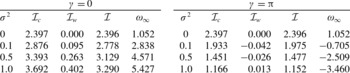
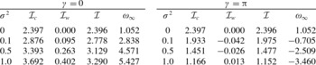
. We list the values of
 ${\mathcal{I}}_{c}$
,
 ${\mathcal{I}}_{w}$
and
 ${\mathcal{I}}$
(the left-hand side of (4.6)) in table 1 for
 $\mathit{Ra}=500$
,
 $\ell =40$
,
 $m=6{\rm\pi}$
and
 $t=0.5$
. Table 1 indicates that
 ${\mathcal{I}}$
increases with an increase in the variance when
 ${\it\gamma}=0$
and decreases with an increase in the variance when
 ${\it\gamma}={\rm\pi}$
. Corresponding values of the growth rate listed in table 1 indicate that larger values of
 ${\mathcal{I}}$
are associated with greater instability and smaller values with less instability. Table 1 further indicates that
 ${\mathcal{I}}_{c}$
is an order of magnitude greater than
 $|{\mathcal{I}}_{w}|$
and therefore sets the magnitude of the net vorticity,
 ${\mathcal{I}}$
. Hence, with an increase in
 ${\it\sigma}^{2}$
, both the increase in
 ${\mathcal{I}}$
for
 ${\it\gamma}=0$
and the decrease in
 ${\mathcal{I}}$
for
 ${\it\gamma}={\rm\pi}$
are related, respectively, to the larger and smaller values of
 $k$
within the boundary layer, as shown in figure 3(c). Permeability gradients play a relatively minor role for the parameter set considered in figure 2.
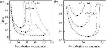
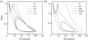
Marginal stability contours for
 ${\it\gamma}=0$
. (a) Influence of
 ${\it\sigma}^{2}$
for
 $m=10{\rm\pi}$
. (b) Influence of
 $m$
for
 ${\it\sigma}^{2}=1$
.

Net vorticity contributions,
 ${\mathcal{I}}_{c}$
,
 ${\mathcal{I}}_{w}$
and
 ${\mathcal{I}}$
, as a function of
 ${\it\sigma}^{2}$
for
 $\ell =40$
,
 $m=6{\rm\pi}$
and
 $t=0.5$
. The corresponding growth rates,
 ${\it\omega}_{\infty }$
, indicate that larger positive values of
 ${\mathcal{I}}$
are associated with greater instability. Net vorticity,
 ${\mathcal{I}}$
, is determined primarily by
 ${\mathcal{I}}_{c}$
for this parameter set because
 ${\mathcal{I}}_{c}/|{\mathcal{I}}_{w}|\gg 1$
.
4.3. Effect of correlation length
For larger values of
 $m$
, the contribution of
 ${\mathcal{I}}_{w}$
to net vorticity is expected to increase because of larger permeability gradients within the boundary layer. To investigate this effect, figure 5(a) plots the marginal stability curves for
 $\mathit{Ra}=500$
,
 ${\it\gamma}=0$
,
 $m=10{\rm\pi}$
and different values of
 ${\it\sigma}^{2}$
. The overall stability behaviour, as a function of
 ${\it\sigma}^{2}$
, is quantitatively different from the case of
 $m=6{\rm\pi}$
considered in figure 2(a). In the case of
 $m=10{\rm\pi}$
considered in figure 5(a), we find that the instability decreases with an increase in
 ${\it\sigma}^{2}$
. This effect is more obvious at times greater than about
 $t>0.4$
, which indicates that the influence of the two modes of vorticity production changes in time due to the change in the thickness of the boundary layer. For
 ${\it\sigma}^{2}=1.1$
, the marginal stability curve splits into two separate unstable regions that continue to diminish with further increase in the variance. Figure 5(b) plots the effect of
 $m$
for
 ${\it\sigma}^{2}=1$
. As
 $m$
is increased from
 $8{\rm\pi}$
to
 $10{\rm\pi}$
the marginal stability curve shrinks substantially. With further increase in
 $m$
to
 $10.4{\rm\pi}$
, the marginal stability curve again splits, similar to the case for
 $m=10{\rm\pi}$
and
 ${\it\sigma}^{2}=1.1$
shown in figure 5(a). The lower branch disappears entirely with further increase in
 $m$
to
 $12{\rm\pi}$
.
The physical basis for the reduced instability at larger values of
 $m$
and
 ${\it\sigma}^{2}$
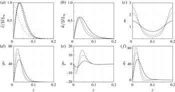
, indicated in figure 5, is explained with the help of figure 6. The profiles for scaled concentration perturbations observed in figure 6(a) are not sensitive to
 ${\it\sigma}^{2}$
. The corresponding peak velocity perturbations are similarly not sensitive to
 ${\it\sigma}^{2}$
, but the profiles move slightly inwards into the boundary layer when
 ${\it\sigma}^{2}$
is increased, as shown in figure 6(b). Permeability profiles plotted in figure 6(c) indicate that
 $k$
undergoes a relatively smaller increase in the neighbourhood of the peak of
 $\tilde{c}/\Vert \tilde{c}\Vert _{\infty }$
with an increase in
 ${\it\sigma}^{2}$
compared with the case for
 $m=6{\rm\pi}$
shown in figure 3(c). Consequently, the increase in the corresponding vorticity contribution,
 $\hat{{\it\eta}}_{c}$
, is relatively smaller for
 $m=10{\rm\pi}$
as shown in figure 6(d) compared with the case for
 $m=6{\rm\pi}$
shown in figure 4(a). The permeability gradients, on the other hand, are now much larger and lead to significantly larger values of
 $\hat{{\it\eta}}_{w}$
with an increase in
 ${\it\sigma}^{2}$
, as shown in figure 6(e). The effect on
 $\hat{{\it\eta}}$
, plotted in figure 6( f), shows that vorticity is now confined to a narrower region of the boundary layer. This results in a decrease in the net vorticity,
 ${\mathcal{I}}=(2.40,2.32,2.23)$
, with an increase in variance,
 ${\it\sigma}^{2}=(0.1,0.5,1.0)$
, which coincides with a corresponding decrease in the growth rate,
 ${\it\omega}_{\infty }=(1.43,1.22,0.70)$
.
Spatial variation of perturbation and vorticity contributions for
 $\ell =40$
,
 $m=10{\rm\pi}$
and
 $t=0.5$
. Lines represent:
 ${\it\sigma}^{2}=0$
(solid),
 ${\it\sigma}^{2}=0.1$
(dashed) and
 ${\it\sigma}^{2}=0.5$
(dash-dotted). Symbols in plot (a) represent the base state.

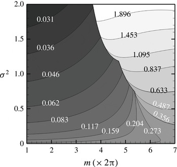
The overall effect of the interaction of the two mechanisms of vorticity production described above is summarized in figure 7, which plots contours of
 $t_{c}$
in the plane of
 ${\it\sigma}^{2}$
and
 $m$
. These results are obtained with the DMA, given by (4.1). Figure 7 indicates that
 $t_{c}$
decreases with an increase in
 ${\it\sigma}^{2}$
for small values of
 $m$
and increases with an increase in
 ${\it\sigma}^{2}$
for larger values of
 $m$
. Transition from one type of behaviour to the other occurs at intermediate values of
 $m$
. A sharp jump in the critical time,
 $t_{c}$
, occurs for large values of
 ${\it\sigma}^{2}$
because the lower of the two stability branches, shown in figure 5, vanishes, and
 $t_{c}$
jumps to the larger value on the upper branch. For smaller values of
 ${\it\sigma}^{2}$
the transition is gradual. Such transitions are associated with the relative strength of the vorticity production mechanisms, see (4.4), related to the magnitude and the gradient of permeability. The mode of instability switches from being dominated by the magnitude of permeability for smaller values of
 $m$
to being dominated by the gradients of permeability for large values of
 $m$
. We note that the effect of mode switching is most prominent when high-permeability regions are located closer to the top boundary,
 $z=0$
, for
 $-3{\rm\pi}/4<{\it\gamma}<3{\rm\pi}/8$
. In this range, the effects of mode switching observed in figures 5 and 7 extend to the onset of nonlinear convection, as described next in § 5. We have also observed similar mode transitioning effects in anisotropic porous media (not shown) where the transition occurs for larger (smaller) permeability wavenumbers with increasing (decreasing) horizontal permeability. We expect these mode switching effects to also occur for steady boundary layers (Hewitt, Neufeld & Lister Reference Hewitt, Neufeld and Lister2014).
Effect of
 ${\it\sigma}^{2}$
and
 $m$
on the critical time for the onset of instability,
 $t_{c}$
, determined by the DMA, (4.1). Numbers indicate the magnitude of
 $t_{c}$
. Grey scale emphasizes the direction of increasing and decreasing values of
 $t_{c}$
, with lighter (darker) colour indicating higher (lower) values.

5. Onset of natural convection
The onset of natural convection, which marks the beginning of a period of enhanced dissolution, occurs in response to perturbation amplification within the linear regime. At the time of convection onset, the flux of
 $\text{CO}_{2}$
into the brine transitions from a diffusive to a convective regime. The critical time for the onset of convection is defined as the minimum time for the onset of convection over all perturbation wavenumbers. The onset of convection is associated with the onset of nonlinear effects that are triggered when the perturbation amplitude becomes sufficiently large. Below we characterize, with the help of two-dimensional numerical simulation, the dependence of the onset time of convection on the amplification of perturbations predicted using linear theory. We show that due to this dependence, the mode switching behaviours in the linear regime are also observed in the onset of convection.
Our method of direct numerical simulation (DNS) is based on the vorticity streamfunction formulation for (2.1) (Riaz et al.
Reference Riaz, Hesse, Tchelepi and Orr2006). We use spectral discretization in the
 $x$
direction, compact finite differences in the
 $z$
direction, and a third-order Runge–Kutta explicit time integration. Periodic boundary conditions are used in the
 $x$
direction. The initial conditions for the DNS are set as
 $u=w=0$
, and
 $$\begin{eqnarray}c(x,z,t_{o})=c^{o}(z,t_{o})+{\it\varepsilon}\cos (\ell x)\tilde{c}_{o}(z),\end{eqnarray}$$
where
 $t_{o}$
is the time at which the system is perturbed,
 $c^{o}(z,t_{o})=\text{erfc}(z\sqrt{\mathit{Ra }/4t_{o}})$
is the base state for the linear stability analysis,
 ${\it\varepsilon}$
is the initial perturbation amplitude,
 $\ell$
is the perturbation wavenumber and
 $\tilde{c}_{o}(z)$
is the initial perturbation defined in (3.12). The minimum amplitude is
 ${\it\varepsilon}=0$
, which cannot lead to instability because of the quiescent initial state,
 $u=w=0$
. The maximum value of
 ${\it\varepsilon}$
is constrained by the requirement
 $c(x,z,t_{o})>0\,\text{for all}~(x,z)$
, to ensure that no unphysical negative values of concentration occur at
 $t=t_{o}$
and beyond. Tilton et al. (Reference Tilton, Daniel and Riaz2013) developed an asymptotic scaling to demonstrate how the onset time of convection approaches infinity as the amplitude goes to zero. They showed that the initial concentration perturbations outside the boundary layer cannot lead to finite onset times because the initial amplitude needs to go to zero in order to satisfy the physical constraint.
5.1. Critical time of convection onset
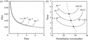
The time at which convection starts is typically associated with the point of deviation of the flux from the diffusive behaviour. The flux of
 $\text{CO}_{2}$
into brine is obtained by integrating the normal concentration gradient across the boundary at
 $z=0$
from
 $x=0$
to the domain width,
 $x=a_{r}$
,
 $$\begin{eqnarray}J(t)=-\frac{1}{a_{r}\mathit{Ra}}\int _{0}^{a_{r}}\left.\frac{\partial c}{\partial z}\right|_{z=0}\text{d}x.\end{eqnarray}$$
The time at which the onset of natural convection occurs is taken to be the time,
 $t_{n}$
, when
 $\text{d}J/\text{d}t=0$
. The flux,
 $J(t)$
, obtained from the DNS for various values of the initial amplitude,
 ${\it\varepsilon}$
, is shown in figure 8(a) for
 $\mathit{Ra}=500$
,
 $\ell =20$
,
 ${\it\sigma}^{2}=0$
,
 $a_{r}=2{\rm\pi}/\ell$
and
 $t_{o}=0.01$
. The symbols in the plot represent the diffusive flux in the linear regime,
 $1/\sqrt{{\rm\pi}\,\mathit{Ra }\,t}$
. Figure 8(a) shows that the flux follows the diffusive path initially. Eventually, nonlinear interactions between the perturbed mode and its harmonics modify the mean concentration to deviate the flux from the diffusive behaviour (Tilton & Riaz Reference Tilton and Riaz2014).
(a) Flux,
 $J(t)$
, for
 $\mathit{Ra}=500$
,
 $\ell =20$
,
 ${\it\sigma}^{2}=0$
and
 $t_{o}=0.01$
for various values of the perturbation amplitude. Symbols represent the flux associated with the diffusive boundary layer. (b) Time for convection onset,
 $t_{n}$
, as a function of
 $\ell$
obtained from DNS (solid lines). Amplification,
 ${\it\Phi}$
, at
 $t_{n}$
is only a function of
 ${\it\varepsilon}$
. The critical onset time,
 $t_{nc}$
, (symbols) occurs on the path of maximum amplification,
 ${\it\Phi}^{\ast }(t)$
, (dashed line) in the linear regime.

The onset time
 $t_{n}$
is plotted as a function of
 $\ell$
in figure 8(b). A critical time for the onset of convection,
 $t_{nc}$
, can be defined as the minimum value of
 $t_{n}$
over all perturbation wavenumbers. In order to associate
 $t_{nc}$
with the dynamics in the linear regime, we define the amplification attained by a given perturbation over a specific time interval,
 $\{t_{o},t\}$
, according to
 $$\begin{eqnarray}{\it\Phi}(t;\ell )=\frac{\Vert \tilde{c}(z,t;\ell )\Vert _{2}}{\Vert \tilde{c}(z,t_{o})\Vert _{2}}=\exp \int _{t_{o}}^{t}{\it\omega}_{2}(t;\ell )\text{d}t.\end{eqnarray}$$
Note that the growth rates,
 ${\it\omega}_{2}$
(IVP), and the perturbation profile,
 $\tilde{c}$
, are obtained using linear theory, while the onset of convection is calculated via DNS. The term on the right in (5.3) indicates that the amplification measures the combined effect of the instantaneous growth rates, summed over a specific period of time. Clearly,
 ${\it\Phi}(t;\ell )$
is a function of
 $t_{o}$
, which is discussed in more detail by Daniel et al. (Reference Daniel, Tilton and Riaz2013). Here we consider a fixed value of
 $t_{o}=0.01$
that is about an order of magnitude smaller than the onset time for instability in homogeneous media. The maximum instantaneous amplification can then be defined as
 $$\begin{eqnarray}{\it\Phi}^{\ast }(t)=\sup _{\ell }\{{\it\Phi}(t;\ell )\}.\end{eqnarray}$$
Tilton & Riaz (Reference Tilton and Riaz2014) show that the amplification based on the linear analysis accurately predicts the nonlinear amplification at the onset of convection because of weak nonlinearity at
 $t_{nc}$
. The critical time for the onset of convection thus occurs along the path followed by
 ${\it\Phi}^{\ast }(t)$
in
 $(t,\ell )$
-space, as shown in figure 8(b) with the dashed line. The minimum level of amplification needed to trigger the onset is also noted for different values of
 ${\it\varepsilon}$
. We next consider how the specific profile of the path of
 ${\it\Phi}^{\ast }(t)$
and its magnitude influence the time for the onset of convection.
5.2. Influence of mode switching on convection onset
The dependence of
 $t_{nc}$
on
 ${\it\varepsilon}$
,
 ${\it\Phi}^{\ast }(t)$
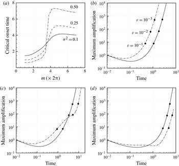
and the heterogeneity parameters is examined in figure 9 for
 $\mathit{Ra}=500$
,
 $t_{o}=0.01$
and
 $a_{r}=2{\rm\pi}/\ell$
. Figure 9(a) shows the effect of variance for three different values of
 ${\it\sigma}^{2}$
and
 ${\it\varepsilon}=10^{-2}$
. In each case,
 $t_{nc}$
transitions from a set of small to large values with an increase in
 $m$
. The transition is gradual when
 ${\it\sigma}^{2}=0.1$
but becomes progressively steeper for larger values of
 ${\it\sigma}^{2}$
. Figure 9(a) further shows that with an increase in the variance,
 $t_{nc}$
decreases to the left of the transition region but increases to the right. This transition is similar to the one observed in figure 7 with respect to the critical time for the onset of instability,
 $t_{c}$
. The behaviour of
 $t_{nc}$
depicted in figure 9(a) is a consequence of the mode switching mechanisms in the linear regime as discussed in § 4.
(a) Influence of permeability variance,
 ${\it\sigma}^{2}$
, on the critical onset time,
 $t_{nc}$
, for
 $\mathit{Ra}=500$
,
 $t_{o}=0.01$
and
 ${\it\varepsilon}=10^{-2}$
. (b–d)
 ${\it\Phi}^{\ast }(t)$
versus time for
 $m=4{\rm\pi}$
,
 $6.5{\rm\pi}$
and
 $12{\rm\pi}$
, respectively, and
 ${\it\sigma}^{2}=0.1$
and
 $0.5$
. Solid symbols mark
 $t_{nc}$
for three different values of
 ${\it\varepsilon}$
.

In order to understand the effect of mode switching on the behaviour of
 $t_{nc}$
observed in figure 9(a), we consider the temporal evolution of
 ${\it\Phi}^{\ast }(t)$
in figure 9(b–d). In figure 9(b), we plot
 ${\it\Phi}^{\ast }(t)$
as a function of time for
 $m=4{\rm\pi}$
and two different values of
 ${\it\sigma}^{2}=0.1$
and 0.5. The critical time for the onset of convection,
 $t_{nc}$
, corresponding to
 ${\it\varepsilon}=10^{-3}$
,
 $10^{-2}$
and
 $10^{-1}$
is marked with symbols. Figure 9(b) shows that for all values of
 ${\it\varepsilon}$
the amplification,
 ${\it\Phi}^{\ast }(t)$
, is greater when the variance is larger. Therefore, the minimum amplification required for the onset is attained more quickly for the case of
 ${\it\sigma}^{2}=0.5$
resulting in an earlier onset time. This explains the behaviour of the decrease in
 $t_{nc}$
with an increase in
 ${\it\sigma}^{2}$
for small values of
 $m$
, as shown in figure 9(b). We note further in figure 9(b) that the amplification needed to trigger the onset of convection for a fixed value of
 ${\it\varepsilon}$
is similar to that in the homogeneous case shown in figure 8(b).
To examine the transition region noted in figure 9(b), we consider the case of
 $m=6.5{\rm\pi}$
in figure 9(c). In this case,
 ${\it\Phi}^{\ast }(t)$
is greater for
 ${\it\sigma}^{2}=0.5$
until about
 $t=3$
. A point of crossover occurs beyond this time where the amplification is greater for the case of
 ${\it\sigma}^{2}=0.1$
. As a consequence of the crossover, we observe that the critical onset time,
 $t_{nc}$
, for various values of
 ${\it\sigma}^{2}$
depends additionally on
 ${\it\varepsilon}$
. The crossover can be attributed to the mode switching effects that are brought about in this case by the shift in the relative strength of vorticity contributions as a result of boundary layer growth. For larger values of
 ${\it\varepsilon}$
,
 $t_{nc}$
occurs earlier for
 ${\it\sigma}^{2}=0.5$
. On the other hand, for smaller values of
 ${\it\varepsilon}$
,
 $t_{nc}$
occurs later for
 ${\it\sigma}^{2}=0.5$
because the level of amplification needed to trigger the onset of convection is attained beyond the point of crossover. Finally, in the case of a large value of
 $m=12{\rm\pi}$
shown in figure 9(d), the crossover occurs relatively early in time. Consequently,
 ${\it\Phi}^{\ast }(t)$
attains the threshold for the onset well beyond the point of crossover for all values of
 ${\it\varepsilon}$
. This explains why
 $t_{nc}$
is delayed with an increase in variance for large
 $m$
, as observed in figure 9(a).
6. Conclusion
With the help of a periodic model for permeability, we developed a framework for describing instability in terms of vorticity mechanisms. We carried out a statistical analysis with respect to the initial conditions and found that the ensemble of growth rates closely resembles a normal distribution with a relatively large spread. We identified stability methods that lead to good agreement with the mean value of the ensemble. We also showed that the growth rate based on the numerical abscissa is unlikely to occur in practice.
We analysed the behaviour of instability with respect to the interactions between permeability and perturbation profiles within the transient boundary layer. We showed that perturbations in the concentration field couple with the magnitude of permeability within the boundary layer to produce vorticity. A second mode of vorticity production is associated with the coupling of the velocity perturbation with the gradients of permeability within the boundary layer. The gradients of permeability become important when the wavelength of permeability oscillation is small compared with the thickness of the boundary layer. Perturbations in the velocity field either enhance or diminish the vorticity produced by the first mode, depending on the permeability phase. The time required by any perturbation to amplify sufficiently and trigger the onset of nonlinear convection depends on the instantaneous contribution of each vorticity mode, which changes in time with an increase in the boundary layer thickness. Vorticity production can transition from one mode to the other in response to small changes in the permeability field when the variance is high, resulting in abrupt changes in the onset time for convection.
We studied the problem for a single value of the Rayleigh number. This is because simple rescaling based on an internal length scale formed using buoyancy velocity and diffusivity can be used to obtain corresponding results at other values of the Rayleigh number, as shown by Riaz et al. (Reference Riaz, Hesse, Tchelepi and Orr2006) and Tilton et al. (Reference Tilton, Daniel and Riaz2013) for the linear regime. This type of rescaling is also appropriate for characterizing the onset of the nonlinear convection as long as the boundary layer does not interact with the bottom aquifer boundary.
Our physics-based analysis provides a robust basis for the evaluation of practical problems. For example, heterogeneity may be characterized by multiple length scales and sharp changes in the permeability field whose effect on the onset of convection can be understood with respect to the interaction of individual vorticity modes. In the case of multiple permeability length scales, we expect mode switching effects to be present depending upon the magnitude of permeability gradients in the boundary layer. In the limit of high permeability and high variance, the periodic model can also account for abrupt changes in permeability.
Acknowledgements
The authors would like to acknowledge Dr N. Tilton for several helpful discussions and the reviewers for insightful comments. This study was supported through a research grant from the Petroleum Institute, Abu Dhabi.