INTRODUCTION
Irrigation is a basic tool for the sustainability of farm production in arid and semiarid areas. However, it competes with other water uses, both consumptive (urban and industrial uses) and non-consumptive (environmental, energy and leisure uses). Together with the scarcity of fresh water, increasing costs and continual world population growth, this justifies the interest in the promotion of improvements in water use efficiency (WUE) within agriculture (Bessembinder et al. Reference Bessembinder, Leffelaar, Dhindwal and Ponsioen2005). This is observed in the increasing concern of institutions, sprinkler manufacturers, engineers and users in improving application uniformity of irrigation water (Louie & Selker Reference Louie and Selker2000; Cavero et al. Reference Cavero, Jiménez, Puig, Faci and Martínez-Cob2008). By doing so, economic benefits could be obtained, water could be saved, and the environmental impact of irrigation could be reduced (Brennan Reference Brennan2008).
When designing an irrigation system, irrigation engineers try to maximize irrigation efficiency (IE), which has been defined by the American Society of Civil Engineers (ASCE) on-farm irrigation committee (Kruse Reference Kruse1978), as the proportion of the volume of irrigation water applied that is taken up by the crop. IE depends on both water losses and uniformity of water distribution (Stern & Bresler Reference Stern and Bresler1983; Tarjuelo et al. Reference Tarjuelo, Carrión and Valiente1994). The best design and management of an irrigation system should minimize water losses and maximize distribution uniformity (Brennan Reference Brennan2008). There are various different types of irrigation system, but sprinkler irrigation is considered to be the most efficient (McLean et al. Reference McLean, Sri Ranjan and Klassen2000; Al-Jamal et al. Reference Al-Jamal, Ball and Sammis2001). However, even here water losses and uniformity of distribution are affected by the environmental conditions during the irrigation event. Wind is the main environmental factor affecting irrigation uniformity, which decreases as wind speed increases (Seginer et al. Reference Seginer, Nir and Von Bernuth1991; Tarjuelo et al. Reference Tarjuelo, Carrión and Valiente1994; Kincaid et al. Reference Kincaid, Solomon and Oliphant1996; Dechmi et al. Reference Dechmi, Playán, Cavero, Faci and Martínez–Cob2003). The heterogeneity of water application can affect the crop yield (Letey et al. Reference Letey, Vaux and Feinerman1984; Ruelle et al. Reference Ruelle, Mailhol, Quinones and Granier2003; Dechmi et al. Reference Dechmi, Playán, Cavero, Martínez-Cob and Faci2004). Most of the studies carried out in relation to this subject show that a lack of uniformity translated into a lower mean yield (Mantovani et al. Reference Mantovani, Villalobos, Orgaz and Fereres1995; Martínez Reference Martínez2004). Knowledge of the influence of uniformity on yield is important for the proper design, management and economic evaluation of an irrigation system (Stern & Bresler Reference Stern and Bresler1983).
Onion (Allium cepa L.; Alliaceae) is the most widely produced and consumed bulb vegetable throughout the world. Onion is used worldwide among all nationalities and cultures and is available in most markets of the world during all seasons of the year. World onion production has doubled in the last 20 years, reaching 58 million tonnes from an area of 3·2 million ha (Food and Agriculture Organization (FAO) 2004). Average world yield increased from 12 t/ha in the early 1960s to 18 t/ha in 2004. Onion can be grown under a wide range of climatic conditions. Production is well-adapted to cool weather conditions with adequate moisture during early growth followed by warm, dry conditions during maturity and curing (Jones & Mann Reference Jones and Mann1963). Spain produces c. 1 000 000 t/year on 23 000 ha, which accounts for one-fifth of the whole European Union (EU) production. This is mainly the result of its high average yield of 47 t/ha (Ministerio de Agricultura, Pesca y Alimentacíon (MAPA) 2006). According to official published data, Albacete produces more onions than any other Spanish province (377 500 t); it also has the largest area given over to onion production (5630 ha) and the largest mean yield (67 t/ha; MAPA 2006). All onion production in Albacete is carried out using sprinkler irrigation systems.
Many studies have been carried out worldwide in relation to the crop water requirements of onion (Martín De Santa Olalla et al. Reference Martín De Santa Olalla, De Juan and Fabeiro1994; Sharma et al. Reference Sharma, Katole and Gautam1994; Wu & Shimabuku Reference Wu and Shimabuku1996; Saha et al. Reference Saha, Khan, Haider and Saha1997; Shock et al. Reference Shock, Feibert and Saunders1998, Reference Shock, Feibert and Saunders2000a; Al-Jamal et al. Reference Al-Jamal, Sammis, Ball and Smeal1999; Bandyopadhyay et al. Reference Bandyopadhyay, Mallick and Rana2003; Kadayifci et al. Reference Kadayifci, Tuylu, Ucar and Cakmak2005; Rajput & Patel Reference Rajput and Patel2006; Kumar et al. Reference Kumar, Imtiyaz, Kumar and Singh2007a). These studies give various water requirements depending on the onion variety, planting density, crop techniques, expected output, local climatic conditions, irrigation scheduling and irrigation system. Doorenbos & Kassam (Reference Doorenbos and Kassam1979) considered that for an optimum production of 35–45 t/ha (bulbs with 100–150 g dry matter (DM)/kg FW), onions needed 350–550 mm of water (10–12 kg/m3). Using a lysimeter, Bossie et al. (Reference Bossie, Tilahun and Hordofa2009) found maximum evapotranspiration values of 51 mm during the initial growth stages (first 20 days), 140 mm during crop development (next 30 days), 145 mm in mid season (next 30 days) and 54 mm during late season (last 20 days). These data differ significantly from those obtained recently by other researchers. When grown in semi-arid climates, such as that used in the present study, onions are considered to have a high water demand. Ells et al. (Reference Ells, Mcsay, Soltanpour, Schweissing, Bartolo and Kruse1993) reported that onions grown under a furrow irrigation system require 1040 mm water to achieve a 59 t/ha yield in the Arkansas River Valley of Colorado. Martín De Santa Olalla et al. (Reference Martín De Santa Olalla, Domínguez-Padilla and López2004) reported that the water requirements in Albacete (Spain) for an optimum yield of 75 t/ha were 602 mm water when using drip irrigation. Drost et al. (Reference Drost, Grossl, Koenig, Camp, Sadler and Yoder1996) obtained 77 t/ha from a sprinkler-irrigated onion crop in Utah with 910 mm of water. Another important aspect is that in Albacete (Spain), seasonal evapotranspiration measured in the lysimeter (893 mm) was higher than the seasonal theoretical crop evapotranspiration (ETc) calculated by the FAO-56 method (833 mm; López Urrea Reference López Urrea, Martín De Santa Olalla, Montoro and López Fuster2009).
As it is highly sensitive to soil water deficit, both bulb yield (BY) and WUE of this crop are reduced when subjected to water deficit (Martín De Santa Olalla et al. Reference Martín De Santa Olalla, De Juan and Fabeiro1994; Kadayifci et al. Reference Kadayifci, Tuylu, Ucar and Cakmak2005; Sarkar et al. Reference Sarkar, Goswami, Mallick and Nanda2008). Doorenbos & Kassam (Reference Doorenbos and Kassam1979) reported that the crop is more sensitive to water deficit during the yield formation period, especially during the period when the bulb is growing quickly. The crop is equally sensitive during transplanting. In the case of a seed crop, the flowering period is also very sensitive to water deficit. During the vegetative growth period, the crop seems to be relatively less sensitive to water deficit. Shock et al. (Reference Shock, Feibert and Saunders2000b, Reference Shock, Feibert and Saunders2007) and Bekele & Tilahun (Reference Bekele and Tilahun2007) confirm these results for onion under irrigation deficits. Irrigation deficit during late bulb formation greatly reduced BY and size grade of onion in Oregon (Shock et al. Reference Shock, Feibert and Saunders2000b). However, a number of experiments carried out in the past by our own research team (Martín De Santa Olalla et al. Reference Martín De Santa Olalla, De Juan and Fabeiro1994), as well as by other teams who worked under different conditions, have led to the suggestion that it is possible to ration water applications on a highly selective basis at particular phenological stages with negligible losses in terms of quantity and quality of final output. Such studies have contributed to increasing the existing knowledge on water use characteristics of onion crops under deficit irrigation with respect to irrigation depth, daily and seasonal evapotranspiration, BY, quality of final yield, water productivity functions developed from yield-evapotranspiration and yield-seasonal irrigation depth (generally, a curvilinear water production function (WPF) is expressed as a second- or third-order polynomial), yield response factor (ky), irrigation WUE (IWUE) and WUE (Martín De Santa Olalla et al. Reference Martín De Santa Olalla, De Juan and Fabeiro1994, Reference Martín De Santa Olalla, Domínguez-Padilla and López2004; Ramos Reference Ramos1999; Al-Jamal et al. Reference Al-Jamal, Sammis, Ball and Smeal2000; Kadayifci et al. Reference Kadayifci, Tuylu, Ucar and Cakmak2005; Sarkar et al. Reference Sarkar, Goswami, Mallick and Nanda2008).
Except for the study by Al-Jamal et al. (Reference Al-Jamal, Ball and Sammis2001), no other references have been found that analyse the agronomic effects of irrigation uniformity on an onion crop. This is important in the context of arid or semiarid areas with limited water resources, such as Albacete (Spain), where water is extracted from aquifers which are in serious danger of over-exploitation.
The present paper analyses how water application through a sprinkler irrigation system influences onion yield and quality, taking into account water application heterogeneity and the effect on ETc.
MATERIALS AND METHODS
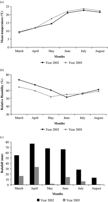
The field experiment was conducted at commercial onion plots irrigated with a permanent sprinkler irrigation system located in Motilleja (Albacete, Spain), during the 2002 (location 39°10′05″N, 1°46′15″W) and 2005 (location 39°10′23″N, 1°47′34″W) irrigation seasons. The local climate is classed as Warm Mediterranean (Papadakis Reference Papadakis1966) characterized by a warm temperature thermal regime (TE) and a dry Mediterranean humidity regime (Me). There is pronounced seasonal variations, with mean temperatures of around 4·5°C in the coldest month (January) and 24–26°C in the hottest month (July). The average annual rainfall in the area is about 320 mm. The weather during 2002 and 2005 is summarized in Fig. 1.
Climate variables during the experimental seasons. (a) Mean temperature, (b) relative humidity and (c) rainfall.

Soils at the experimental plots are representative of the area. They are classified as a petric calcisol (at the 2002 location) and a haplic calcisol (2005 location; FAO 1998) and have a clay loam texture in the first 0·35 m of the soil profile. The average soil depth of the plots involved in the experiment was 0·65 m and was limited by the development of the petrocalcic and calcic horizons which are found to be more or less fragmented. Moreover, the soil is basic (pH=8·6–8·8), poor in organic matter (OM=10–20 g/kg), total nitrogen (N=0·4–1·0 mg/g), and assimilable phosphorus (P=0·05–0·08 mg/g); and also is rich active limestone and potassium (K=0·3–0·6 mg/g).
In order to obtain total available water (TAW), as the difference between field capacity (FC) and permanent wilting point (PWP), the empirical methods of Gupta & Larson (Reference Gupta and Larson1979) and Rawls et al. (Reference Rawls, Brakensiek and Saxton1982) were used. Water content at FC was 0·34 m3/m3 and water content at the wilting point was 0·21 m3/m3. TAW was estimated as 52 mm for the 0·40 m root zone. The readily available water (RAW) was obtained as RAW=TAW×p, where a permissible soil water depletion level (p) of 0·35 was adjusted for an average ETc of 5·83 mm/day during the whole crop growing cycle. As a result, RAW=18·2 mm. This value was taken as the maximum irrigation dose to be applied during the experimental season.
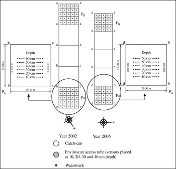
Two experimental plots were selected each study year from a commercial field: Plot A (PA), in which water was heterogeneously applied, and Plot B (PB), used as the reference plot. Sprinkler spacing was 17·2×16·4 m in 2002 and 15·0×15·0 m in 2005, in both PA and PB. Sprinklers were provided with different diameter nozzles in PA and maintained with the same nozzle combination (4·4+2·4 mm diameter) throughout the crop growing cycle in PB (Fig. 2). Sprinklers were placed 2·40 m high and operated at a pressure of c. 300 kPa.
Layout of the experimental plots. a=sprinkler with double nozzle 4·4 mm+2·4 mm in diameter (discharge=1671 l/h; throw=14·5 m); b=sprinkler with double nozzle 5·2 mm+3·2 mm in diameter (discharge=2481 l/h; throw=15·4 m); c=sprinkler with a single nozzle 4 mm in diameter (discharge=1075 l/h; throw=13·8 m); d=sprinkler with a single nozzle 3·2 mm in diameter (discharge=681 l/h; throw=10·2 m); PA, plot A; PB, plot B.

Both PA and PB were divided into 25 subplots (11·3 m2 each in 2002; 9·0 m2 each in 2005), in order to study not only the distribution of water when it was applied with a different degree of uniformity but also the yield obtained.
The method used for daily irrigation scheduling was the simplified water balance in the root zone, calculated by means of software devised by our own team and developed according to the methodology formulated by Doorenbos & Pruitt (Reference Doorenbos and Pruitt1977) and Doorenbos & Kassam (Reference Doorenbos and Kassam1979), updated in Allen et al. (Reference Allen, Pereira, Raes and Smith1998) and Pereira & Allen (Reference Pereira, Allen, van Lier, Pereira and Steiner1999). Reference evapotranspiration (ET0) was calculated on a daily basis by means of Penman–Monteith's semi-empirical formula (Allen et al. Reference Allen, Pereira, Raes and Smith1998), using data from an agrometeorological station located in Motilleja (Albacete, Spain) (39°10′0″N, 1°46′7″W). Kc values were obtained from Allen et al. (Reference Allen, Pereira, Raes and Smith1998) and local experience (López Urrea et al. Reference López Urrea, López Córcoles, López Fuster, Fabeiro and Martín De Santa Olalla2001; Martín De Santa Olalla et al. Reference Martín De Santa Olalla, Domínguez-Padilla and López2004; Ortega et al. Reference Ortega, De Juan and Tarjuelo2005) with the dates and duration of each phenological stage adapted to those observed in the area in the 2002 and 2005 growing seasons. Kc values adopted during the growing season were: 0·5 during the establishment stage (15 March–12 May in 2002 and 16–30 May in 2005), from 0·5 to 1·0 during the development stage (13 May–16 June in 2002 and 31 May–27 June in 2005), 1·0 during the bulb growth stage (yield formation) (17 June–6 August in 2002 and 28 June–7 August in 2005) and from 1·0 to 0·6 during the ripening stage (7–28 August in 2002 and 8–25 August in 2005). The expression of the simplified water balance used was In=ETc−Pe, where In is net irrigation requirements, ETc was the result of the expression ETc=ET0×Kc and Pe is the effective precipitation, estimated as 0·7 of total rainfall (Doorenbos & Pruitt Reference Doorenbos and Pruitt1977; Reca et al. Reference Reca, Roldán, Alcaide, López and Camacho2001; Pulido et al. Reference Pulido-Calvo, Roldán, López-Luque and Gutiérrez-Estrada2003). Scheduling began with soil at FC due to irrigation. When onion ETc was greater than Pe, the soil water reserve was decreased by ETc–Pe until it reached the RAW level; then a net volume of irrigation equal to RAW was applied. This way, the soil returned to its initial water content.
The two experimental plots (PA and PB) were evaluated, over the crop growth period, during the two seasons studied. Evaluations were carried out following not only the Merriam & Keller (Reference Merriam and Keller1978) and Merriam et al. (Reference Merriam, Shearer, Burt and Jensen1980) methodologies but also the ISO 15886-3 standard (ISO 2004). The irrigation events evaluated represented half of 30 irrigation events that took place in 2002, and 0·42 of 26 events in 2005. The coefficient of uniformity (CU) (Christiansen Reference Christiansen1942; Keller & Bliesner Reference Keller and Bliesner1990) was computed from the amount of water collected in the 25 catch cans placed in each subplot:

where CU is the Christiansen uniformity coefficient (given as a number between 0 and 100), Wi is the water depth collected by a catch can i (in ml), MWD is the mean water depth collected in the catch cans (ml) and nc is the number of catch cans.
Pressure was continuously measured during the irrigation events using a gauge pressure transmitter (Druck PTX 1400, Druck Ltd., Leicester, UK), calibrated previously to use (range 0–600 kPa, accuracy ±0·01).
The discharge-pressure sprinkler curve was measured in the laboratory, using an electromagnetic flow meter (accuracy±0·02) and a similar pressure transmitter to the one used at the experimental plots. This way, the discharged flow during the irrigation events could be obtained by measuring pressure evolution over time at the plots.
The existing space between sprinklers was divided into equal parts so catch cans were placed forming a grid collector array. The collected water volume was measured using graduated test tubes (accuracy±0·03). The CU was estimated using the data collected.
Soil water potential was measured using 12 Watermark™ sensors (Irrometer Co., Riverside, CA, USA) placed at depths of 100, 200, 300, 400, 500 and 600 mm in PA, six of them next to one side of the plot and the other six next to the other side (Fig. 2). These data, registered every 8 h, were used daily to locate the zero flux plane (ZFP) or the depth within the soil profile at which the hydraulic gradient is zero (Khalil et al. Reference Khalil, Sakai, Mizoguchi and Miyazaki2003).
Soil moisture content was measured by means of a sensor that utilizes the frequency domain reflectometry (FDR) technology (Enviroscan™, Sentek Pty Ltd., Stepney, Australia). Four probes were placed in each side of PA, monitoring soil water down to 400 mm; sensors were placed at depths of 100, 200, 300 and 400 mm, data were registered every 10 min and the mean of those values registered every hour was stored (Fig. 2).
Onions (cv. ‘Himalaya’) were directly sowed on 20 February in 2002 (416 667 plants/ha) and row-planted on 16 May in 2005 (307 692 plants/ha). Harvest took place at the end of August both years (28 August 2002 and 25 August 2005). The rest of the farm work and crop operations followed the tradition carried out by the farmers in the area (De Juan et al. Reference De Juan, Ortega and Tarjuelo2003). Plots were fertilized annually with 210 kg N/ha, 200 kg P2O5/ha and 180 kg K2O/ha. During the experimental seasons a control of weeds was conducted based on chemical control by pre-emergence treatment or pre-transplant with pendimethalin (330 g/l) at a dose of 4 l/ha. There was a second treatment with oxifluorfen (48%) at a dose of 1 litre/ha when the crop had between two and five leaves. With regard to disease control, two treatments of mancozeb (80%), at a dose of 2·5 kg/ha and applied 100 and 120 days after transplantation (115 and 135 days from sowing in 2002), were used to prevent rust and mildew of onion. Some problems regarding insects (Agrotis segetum Schiff) were detected, which were controlled with azadirachtin (3·2%) at a dose of 1·5 l/ha.
Throughout the 2 years of study, the crop growing stages were monitored, by using the phonological scale proposed by Feller et al. (Reference Feller, Bleiholder, Burhr, Hack, Hess, Klose, Meier, Stauss, Van Den Boom and Weber1995). Yield and its components were determined for each subplot in PA and PB after manual harvest of one-third of the area of each and the bulbs classified by diameter using the main marketing criteria of the country viz., the Spanish Standard Classification of fresh bulbs (MAPA 1992): S1 (diameter >90 mm), S2 (diameter 90–70 mm), S3 (diameter 70–40 mm), S4 (diameter 40–20 mm) and S5 (diameter ⩽20 mm) and the proportion in each class determined.
In 2005, additional qualitative characteristics of the harvested onions were assessed in the laboratory. These were the DM content of both bulbs and leaves, estimation of firmness using a texture analyser (TA.XT Plus, Stable Micro Systems Ltd., Godalming, Surrey, UK) with a cylinder probe of 3 mm diameter, estimation of soluble solid content using a digital refractometer (Palette PR-100, Atago Co. Ltd., Itabashi-ku, Tokyo, Japan), measurement of pH using a pH meter (micro pH 2001, Crison Instruments S. A., Alella, Barcelona, Spain) and determination of total acidity by potentiometric titration with a 0·1 N standardized sodium hydroxide (NaOH) solution.
The statistical analyses were performed using Statgraphics Plus™ software (v. 5.1 for Windows, Statistical Graphics Corp., Herndon, VA, USA) and ArcGIS™ (v. 9.0, ESRI, Redlands, CA, USA). The analyses carried out included non-linear regressions in order to determine yield as a function of total water received by the crop (mm) and to estimate the Kc curve in addition to a one-way analysis of variance (ANOVA) for yield, yield components and firmness. In order to determine the significant differences between group means in the ANOVA, accuracy of the ordinary kriging procedure used at the geostatistics analysis was evaluated using the standardized mean absolute error and the root-mean-square standardized error (Webster & Oliver Reference Webster and Oliver2001; Johnston et al. Reference Johnston, Ver Hoef, Krivoruchko and Lucas2003). The experimental semivariogram showed the best fit with spherical models (Johnston et al. Reference Johnston, Ver Hoef, Krivoruchko and Lucas2003; Zhang Reference Zhang2005).
RESULTS
Uniformity of water application
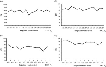
Figure 3 presents the evolution of the CU throughout the irrigation events tested in both years of study.
Evolution of the coefficient of uniformity through the irrigation events tested. 2002 (a and b), 2005 (c and d), plot A (a; c), plot B (b and d). PA, plot A; PB, plot B; CU, Christiansen coefficient of uniformity; ni, number of the irrigation event tested.

The CU in PA ranged from 65 to 82 in 2002 and from 59 to 79 in 2005, while that in PB ranged from 78 to 92 in 2002 and from 79 to 93 in 2005. The variability in the results of each irrigation season and each nozzle combination is mostly due to random variations of the wind conditions during each irrigation event. However, the results show clear differences between the experimental plots. Thus, in PA, with a nozzle combination designed to produce heterogeneity, the values of CU obtained were below 80, in contrast to those on PB (the reference experimental plot) which had CU values usually higher than 80.
Estimation of actual evapotranspiration (ETa)
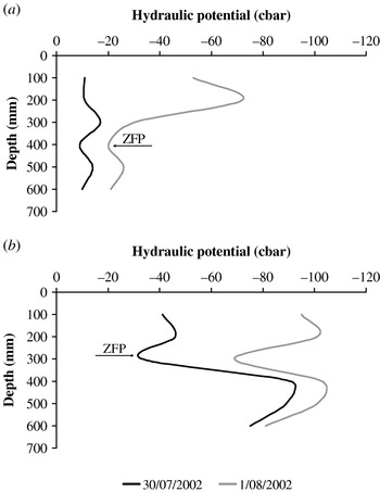
A comparison was made between the theoretically estimated ETc and ETa in the two experimental seasons. First, the ZFP was located daily within the soil profile (Fig. 4), by monitoring of the soil water potential. This information, plus measurements of the crop roots, was used to set the maximum depth from which the crop could have extracted water. Afterwards, daily soil moisture differences at that set depth were quantified by means of the data registered by the EnviroScan™. ETa (mm) was estimated using the following water balance equation:

where In is the net irrigation required (mm), Pe is the effective precipitation (mm) and ΔS is the change in soil moisture storage (mm).
Hydraulic potential within the soil profile after the irrigation event of 29 July 2002 in plot A (PA). (a) Side of the plot on which more irrigation water was received. (b) Side of the plot on which less irrigation water was received. ZFP, zero flux plane.

These estimations were carried out at both sides of PA (Fig. 2). Data registered next to the sprinklers with a higher rainfall intensity were used to estimate crop water requirements in the absence of water deficit, and data registered next to the opposite sprinklers were used to estimate crop water needs under conditions of water deficit.
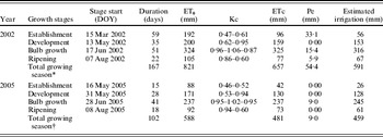
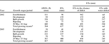
Irrigation scheduling through the growth stages is detailed in Table 1. Table 2 shows seasonal onion ETa measured, seasonal onion ETc calculated by standard FAO methodology and water applied with both irrigation and rainfall.
Irrigation scheduling

* Emergence: 15 March. Harvest: 28 Aug.
† Transplant: 16 May. Harvest: 25 Aug.
DOY, day of year; ET0, reference evapotranspiration (Penman–Monteith); ETc, theoretical crop evapotranspiration (Allen et al. Reference Allen, Pereira, Raes and Smith1998); Pe, effective precipitation.
Evapotranspiration estimation

* Emergence: 15 March. Harvest: 28 Aug.
† Transplant: 16 May. Harvest: 25 Aug.
‡ Estimation assuming the ETc values in the period of time in which no data to calculate ETa+ were available.
AWD, accumulated water depth in plot A (PA) considering all the irrigation events that took place in the study period; Pe, effective precipitation; ETc, theoretical crop evapotranspiration (Allen et al. Reference Allen, Pereira, Raes and Smith1998); ETa, actual crop evapotranspiration; ETa in the absence of deficit=ETa estimated next to the side of the plot on which more irrigation water was received (next to the sprinklers with double nozzle 5·2 mm+3·2 mm in diameter); ETa with water deficit=ETa estimated next to the side of the plot on which less irrigation water was received (next to the sprinklers with a single nozzle 4 mm in diameter in 2002 and 3·2 mm in diameter in 2005); nd, no data available.
As shown in Table 2, ETc and crop water requirements in the absence of water deficit increased rapidly during the first growth stages due to the canopy growth and increasing ET0. Peak ETc and ETa in the absence of water deficit were reached around 20 July and then declined following the general decrease in ET0 as the agronomic cycle advanced. As shown in Table 2, between 30 May and 18 August 2002, ETa in the absence of water deficit was 22 mm over the accumulated ETc value (491 v. 469 mm). In contrast, ETa in conditions of water deficit was 187 mm below ETc (282 v. 469 mm). In 2005, between 29 May and 25 August, ETa in the absence of water deficit was more similar to ETc, although the accumulated value was 14 mm over ETc (458 v. 444 mm). Correspondingly, ETa in conditions of water deficit was 202 mm below the ETc value for the same period of time (242 v. 444 mm). ETa− represented 0·56 of ETa in the absence of water deficit in both 2002 and 2005. This is because ETa in the absence of water deficit corresponds to a situation of maximum evapotranspiration, in contrast to the ETa in conditions of water deficit. If it is assumed that ETa in the absence of water deficit=ETc in the period of time without EnviroScan™ data, then in 2002 ETc was estimated to be 657 mm and ETa in the absence of water deficit was 679 mm. In 2005, ETc and ETa in the absence of water deficit were estimated as 481 and 495 mm, respectively.
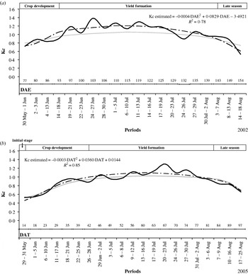
The crop coefficient values shown in Fig. 5 were calculated using the FAO-56 Penman–Monteith equation (Kc=ETa in the absence of water deficit/ET0). The values measured were adjusted to a second-order polynomial function, where the independent variables were days after emergence (DAE) of the seedling in 2002 and days after transplanting (DAT) in 2005.
Comparison between the theoretical and the estimated Kc. (a) 2002 and (b) 2005. Kc, crop coefficient; theoretical Kc, Kc used in the theoretical irrigation scheduling; Kc estimated, relationship between ETa+ and ET0; DAE, days after emergence; DAT, days after transplanting; R 2, coefficient of determination.

Relationship between the water received by the crop and the crop yield
The WPF represents the relationship between crop yield and seasonal water applied (Al-Jamal et al. Reference Al-Jamal, Sammis, Ball and Smeal2000). A non-linear response indicates that not all of the water was used by the crop because some was lost by deep drainage (for example, water application heterogeneity). Generally, a curvilinear WPF is expressed as a second- or third-order polynomial (Hexem & Heady Reference Hexem and Heady1978). This WPF can be useful to determine the capacity of irrigation systems and irrigation amount and timing, as well as to compare relative WUEs. Because WPF varies according to the management skills of the irrigator and the type of irrigation system, no single WPF can be determined for a crop.
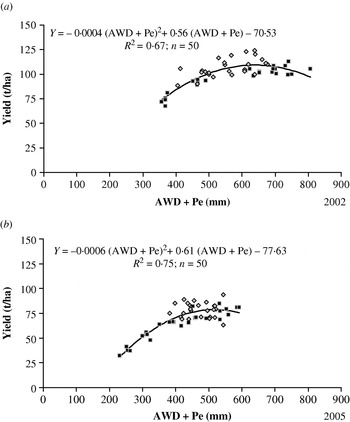
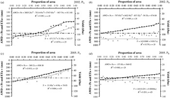
In the present paper, the total water received by the crop was estimated as the accumulated water depth (AWD), considering all the irrigation events from the emergence/transplant plus the Pe. It has to be mentioned that evaporation and drift losses (EDL) were similar in all the studied plots (mean value of 0·09 and that Pe represented 54 and 9 mm in 2002 and 2005, respectively (data not shown). The relationship between yield and AWD+Pe has been adjusted to second-degree polynomial functions, which best fit the data. The models obtained explained 0·67 and 0·75 of BY variability in 2002 and 2005, respectively (Fig. 6). However, the R 2 of these models improves if only PA data is used for estimation. In that case, they would explain 0·91 of BY variability in both 2002 and 2005 (Table 3).
Relationship between the water received by the crop and the yield obtained in each subplot. (a) 2002 and (b) 2005. PA, plot A; PB, plot B; Y, yield; AWD, accumulated water depth considering all the irrigation events from the emergence/transplant; Pe, effective precipitation; R 2, coefficient of determination; n, sample size.

Regression models explaining yield as a function of total water depth received by the crop from the emergence/transplant at the experimental plot A (PA)

Y, yield (t/ha); AWD, accumulated water depth considering all the irrigation events from the emergence/transplant (mm); Pe, effective precipitation (mm); R 2, coefficient of determination (%); n, sample size.
Figure 7 shows the BY associated with AWD+Pe values of each subplot in decreasing order. Thus, the values of BY and AWD+Pe v. the proportion of area are shown (Fig. 7). As a general rule, in those subplots which received water to maintain ETa in the absence of water deficit, no greater BY was obtained. The higher uniformity of water distribution in PB was translated into a higher uniformity of yield distribution.
Water and yield distribution. 2002 (a and b), 2005 (c and d), plot A (a and c), plot B (b and d). PA, plot A; PB, plot B; AWD, accumulated water depth considering all the irrigation events from the emergence/transplant; Pe, effective precipitation; ETa+, actual crop evapotranspiration estimated next to the side of PA on which more irrigation water was received; Y, yield; R 2, coefficient of determination; n, sample size.

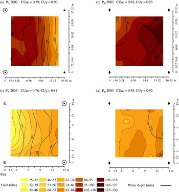
Figure 8 shows both the contour maps of kriged yield estimates and the isolines described by the AWD for all the studied plots. The best yield distributions were observed at PB (Fig. 8 b, d) which confirms the relationship between the uniformity of water applied and yield uniformity.
Superposition of the isoline maps of water depth collected by the catch cans in all the tested irrigation events (mm) and the onion yield (t/ha) obtained. 2002 (a and b), 2005 (c and d), plot A (a and c), plot B (b and d). PA, plot A; PB, plot B;  , sprinkler with double nozzle 5·2+3·2 mm in diameter; ▴, sprinkler with a single nozzle 4 mm in diameter; ◆, sprinkler with double nozzle 4·4+2·4 mm in diameter;
 , sprinkler with a single nozzle 3·2 mm in diameter; CUac, accumulated coefficient of uniformity, estimated with the accumulated depth of water in the irrigation events tested; CUy, yield coefficient of uniformity.

IWUE
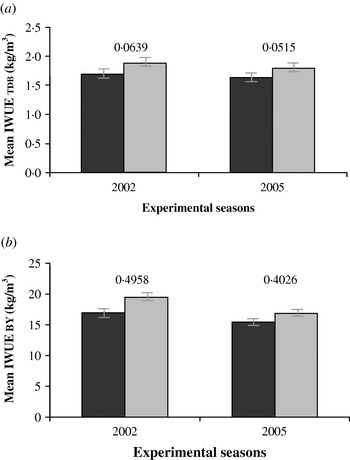
IWUE (t/m3) was estimated by dividing BY (onion DM content of 100 g/kg) by AWD+Pe (IWUEBY) and total dry biomass (TDB) by AWD+Pe (IWUETDB), for all subplots (Fig. 9). The difference between PA and PB is statistically significant in both 2002 and 2005. The highest IWUE was obtained, in both years, in the control plot (PB).
(a) IWUE regarding TDB (IWUETDB) in the two experimental seasons; (b) IWUE regarding BY (IWUEBY) in the two experimental seasons. PA, plot A; PB, plot B. The numbers above each pair of columns are the s.e.d.

BY and harvest quality
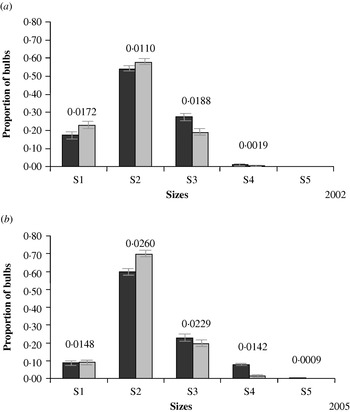
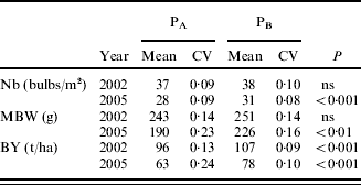
The mean values and the coefficient of variability (CV) of BY and yield components (number of bulbs/m2 (Nb) and mean bulb weight (MBW)) are shown in Table 4. The obtained yield for the experimental plot PA in each experimental season was similar to the obtained yield in the neighbouring areas for similar crop management. There were significant differences between PA and PB in 2002 for the BY values, and in 2005 for Nb, MBW and BY. In 2005, the higher Nb and MBW values were translated into a greater BY in PB (Fig. 10).
Proportion of bulbs regarding size. (a) 2002 and (b) 2005. PA, plot A; PB, plot B; S1, diameter >90 mm; S2, diameter 90–70 mm; S3, diameter 70–40 mm; S4, diameter 40–20 mm; S5, diameter ⩽20 mm.The numbers above each pair of columns are the s.e.d.

Mean and coefficient of variation of yield and yield components

PA, plot A; PB, plot B; CV, coefficient of variation; Nb, number of bulbs/m2; MBW, mean bulb weight; BY, yield of fresh bulbs; ns, not significant.
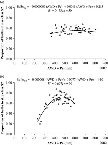
Bulb grading is an important parameter associated with the post-harvest quality (processing) of onions. In both seasons, onion bulbs 70–90 mm in diameter (S2) were of a higher commercial value. Figure 11 shows the relation between AWD+Pe and the proportion of bulbs in class S2. The proportion of S2 bulbs decreased with AWD+Pe in excess of 595 mm in 2002 and in excess of 460 mm in 2005.
Relationship between the water received by the crop and the proportion of bulbs with sizes between 70 and 90 mm in diameter (S2) obtained in each subplot. (a) 2002 and (b) 2005. PA, plot A; PB, plot B; AWD, accumulated water depth considering all the irrigation events from the emergence/transplant; Pe, effective precipitation; R 2, coefficient of determination; n, sample size.

There were no statistically significant differences between PA and PB (P<0·05) in bulb moisture content. Mean bulb moisture contents ranged from 907 (PA 2005) to 917 g water/kg onions (PA 2002).
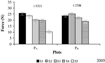
Bulb firmness varies with bulb size (Fig. 12). More force had to be exerted in order to break the first layer of the larger onions. Statistically significant differences between the groups of bulbs created by the treatments imposed were possibly more to do with size itself than with the water received by the crop. No significant differences were found between PA and PB for the total soluble solids, pH and total acidity of onion bulbs.
Onion bulb firmness 2005. PA, plot A; PB, plot B; S1, diameter >90 mm; S2, diameter 90–70 mm; S3, diameter 70–40 mm; S4, diameter 40–20 mm; S5, diameter ⩽20 mm.The numbers above each pair of columns are the s.e.d.

DISCUSSION
Evapotranspiration
The obtained values of seasonal ETc and ETa in the absence of water deficit are significantly different from those provided by Doorenbos & Kassam (Reference Doorenbos and Kassam1979), Drost et al. (Reference Drost, Grossl, Koenig, Camp, Sadler and Yoder1996) and Bossie et al. (Reference Bossie, Tilahun and Hordofa2009). In a previous study conducted in the same area of Albacete (Spain), Martín De Santa Olalla et al. (Reference Martín De Santa Olalla, Domínguez-Padilla and López2004) confirms the achievement of production of 75 t/ha with the application of 602 mm of water through drip irrigation. In the same area, more recent studies, López Urrea et al. (Reference López Urrea, Martín De Santa Olalla, Montoro and López Fuster2009), obtained values of seasonal crop evapotranspiration estimated by both FAO and lysimeter measures, of around 833 and 893 mm, respectively.
The ETc values obtained depend on the onion variety, planting density, crop techniques, expected output, local climatic conditions and the irrigation system.
The theoretical Kc curve used in the present work to schedule the irrigation events was based on a Kc value for each of the four growth stages. When comparing this curve and that belonging to the estimated Kc (polynomial) (Fig. 5), the values used are observed to be a little lower, especially during yield formation (Fig. 5 a, b). At the late-season stage, the estimated Kc curve was a little below the theoretical Kc in 2002 (Fig. 5 a). However, in 2005, both curves were similar (Fig. 5 b). Several Kc values appear in the existing literature depending on the onion variety, crop planting or sowing date, crop development rate, growing season length, soil evaporation, crop techniques and climate conditions. For example, Bandyopadhyay et al. (Reference Bandyopadhyay, Mallick and Rana2003) provided Kc ini, Kc mid and Kc end values of 0·52, 1·04 and 0·87, respectively, in a humid tropical climate in Gayeshpur (eastern India). Al-Jamal et al. (Reference Al-Jamal, Sammis, Ball and Smeal1999) provided a Kc curve correlated to growing degree days. That research was conducted in Farmington (New Mexico) using sprinkler irrigation, and Kc values at the start, middle and end of growth were 0·43, 1·09 and 0·56, respectively. Bossie et al. (Reference Bossie, Tilahun and Hordofa2009) gave a consistent rise from 0·51 to 1·04 during 20–60 DAT. During the mid-season stage, Kc values of onion decreased slightly from 1·04 to 0·95. The crop coefficient declined rapidly to 0·46 during the last stage, 80–100 DAT in the Central Rift Valley of Ethiopia. Recent studies conducted in Albacete provide Kc values derived from lysimeter measurements of 0·65, 1·20 and 0·75 at the start, middle and end of growth (López Urrea et al. Reference López Urrea, Martín De Santa Olalla, Montoro and López Fuster2009). The dual crop coefficient (Kcb) derived from lysimetric measurements were 0·60, 1·10 and 0·65 at the start, middle and end of growth.
Thus, the obtained Kc values are of use in semiarid regions that have similar crop characteristics to those described in the present work. The current values are more accurate than those described in most of the references.
Relationship between the water received by the crop and the crop yield
In the present study, a quadratic relation between AWD+Pe and the BY was obtained (Fig. 6), which could be caused by poor soil aeration and leaching of nutrients when having an excessive soil moisture content.
Many studies relate crop yield and water received by the crops, taking uniformity of water application into account. However, the results show very different R 2 values. Thus, Li & Rao (Reference Li and Rao2000) concluded that sprinkler uniformity, measured on a 2×2 m square grid, had little effect on the yield of a winter wheat cultivated in Beijing (China). The linear regression of yields on irrigation depths led those authors to equations with R 2 values of 0·06 and even lower. On the contrary, Martínez (Reference Martínez2004) obtained an R 2 value of 0·83 in a maize crop and Ayars et al. (Reference Ayars, Hutmacher, Hoffman, Letey, Ben-Asher and Solomon1990) reached 0·96 in sugar beet. In other studies, relationships between onion yield and the total depth of water received by the crop were obtained, without considering the heterogeneity of irrigation water applied. Irrigation scheduling in those studies was performed on the basis of a management-allowed deficit. The abovementioned relationship is explained by statistically significant second-degree polynomial functions, with R 2 values that range from 0·66 to 0·99 (Martín De Santa Olalla et al. Reference Martín De Santa Olalla, De Juan and Fabeiro1994; Ramos Reference Ramos1999; Al-Jamal et al. Reference Al-Jamal, Sammis, Ball and Smeal2000; López Urrea et al. Reference López Urrea, López Córcoles, López Fuster, Fabeiro and Martín De Santa Olalla2001).
Comparing the ungraded onion yields obtained during the 2002 and 2005 growing seasons indicated that higher yield is possible when AWD+Pe increases from 350 to 639 mm in the 2002 growing season and from 215 to 518 mm in 2005. These data vary depending on weather conditions, as well as on crop growth stages and locations (Al-Jamal et al. Reference Al-Jamal, Sammis, Ball and Smeal2000).
IWUE
The values of IWUEBY are greater than those described by Doorenbos & Kassam (Reference Doorenbos and Kassam1979), who estimate it as 8–10 kg/m3 for bulbs containing 850–900 g water/kg onion bulbs. These values are more similar to the results obtained by Martín De Santa Olalla et al. (Reference Martín De Santa Olalla, De Juan and Fabeiro1994) in an experiment carried out in Albacete. These last authors suggested IWUETDB and IWUEBY values of 0·99 and 9·57 kg/m3, respectively, for a treatment in which 0·80 of the crop water needs were satisfied on the basis of the ETc estimation, values of 1·21 and 11·16 kg/m3, respectively, when the water needs were fully satisfied and values of 1·56 and 13·83 kg/m3, respectively, when the water received by the crop exceeded the ETc by 0·20. The values of IWUEBY obtained in the present study are higher than those obtained with onion crops by other authors (Ells et al. Reference Ells, Kruse, McSay, Neal and Horn1986, Reference Ells, Mcsay, Soltanpour, Schweissing, Bartolo and Kruse1993; Al-Jamal et al. Reference Al-Jamal, Ball and Sammis2001) using different irrigation systems (sprinkler, trickle and furrow irrigation systems).
The IWUE values give a more complete analysis of water resource use. This information can be used to inform the selection of the irrigation systems and the irrigation management system used.
BY and harvest quality
In general, mean bulb size and weight reduced significantly with the decrease in irrigation depth, which suggests an effect of water shortage (Doorenbos & Kassam Reference Doorenbos and Kassam1979; Woldetsadik et al. Reference Woldetsadil, Gertsson and Ascard2003; Martín De Santa Olalla et al. Reference Martín De Santa Olalla, Domínguez-Padilla and López2004; Kumar et al. Reference Kumar, Imtiyaz and Kumar2007b). Begum et al. (Reference Begum, Malik, Rahman, Anowar and Khan1990) observed that transpiration, photosynthesis and growth are lowered by mild water deficit and the plants produce smaller bulbs.
The proportion of bulbs in different size classes is a quality indicator having great influence on the final yield price. Martín De Santa Olalla et al. (Reference Martín De Santa Olalla, Domínguez-Padilla and López2004) also reported higher proportions of large bulbs in the presence of optimum soil moisture, whereas water storage during the crop growing period led to higher proportions of smaller bulbs.
The total amount of water the crop requires to maximize the proportion of bulbs of a higher commercial value (Fig. 11) is below the required AWD+Pe to obtain the maximum BY (Fig. 6).
Lai et al. (Reference Lai, Chen, Shanmugasundaram and Tsov1994) reported total soluble solids of different onion cultivars at different harvest times, to range 56–102 g DM/kg. Although Chopade et al. (Reference Chopade, Bansode and Hiwase1998) and Kumar et al. (Reference Kumar, Imtiyaz and Kumar2007b) reported higher total soluble solids in onion with optimum water and fertilizer application, in contrast, Orta & Ener (Reference Orta and Ener2001) found no significant effect of irrigation on total soluble solids of onion bulbs. According to Namesny (Reference Namesny1996), a greater soluble solid content indicates a higher storage success, because of greater resistance to sprouting and greater disease resistance.
The main conclusions from the present work are that onions grown under deficit irrigation, caused by the irrigation heterogeneity of a sprinkler irrigation system, have lower ETa rates, lower yields and smaller mean bulb sizes. In both years, the seasonal water applied and marketable yield of onion crop exhibited quadratic relationships. Onion attained maximum marketable yields of 107 and 78 t/ha with seasonal water applications of 639 and 518 mm, respectively, and thereafter tended to decline. Kc values derived from water balance measurements are similar to those recommended by FAO. The IWUE for the yield of fresh bulbs ranged from 15 to 19 kg/m3, and was greater in those subplots irrigated with higher distribution uniformity. A higher proportion of bulbs in the largest commercially valuable size (S2, 90–70 mm diameter) was obtained at a total water depth (AWD+Pe), slightly lower than that necessary to reach maximum yield. No statistically significant differences were observed between the mean values of the main quality parameters studied in the two experimental plots (PA and PB). The results of the present study can be used to inform the economic costs and benefits of sprinkler irrigation systems both during design and management of irrigated fields.
The authors wish to express their gratitude to the ‘Ministerio de Educación y Ciencia’ (MEC) and the European Social Fund (ESF), for funding the AGL2004-06675-C03-01/AGR and the AGL2007-66716-C03-03 projects of the R&D National Plan. They would also like to thank the ‘S. A. T.’ of Motilleja (Albacete, Spain) for providing the products and facilities needed to carry out this experiment.