

Introduction
Alfalfa (Medicago sativa L.) is one of the most disseminated forage legumes in the temperate regions of the world. It can be used for hay, silage and pasture. With the intensification of milk and meat production systems, there is an increased need to investigate the potential use of alfalfa as a source of feed for cattle in the tropics. Alfalfa can contribute to the productivity and profitability of milk and meat production systems as a result of its symbiotic nitrogen fixation, its ability to mobilize nutrients from the deepest layers of the soil, its high nutritional quality and forage productivity. However, there has been little focus on the potential use of alfalfa cultivars in tropical regions. The utilization of adapted cultivars in combination with adequate herbage management practices is important for the improvement of pasture productivity, quality and persistence.
Genetic evaluation of perennial forage species usually takes several years with repeated samples having to be taken from the same plant. This, in addition to missing data, makes statistical analyses quite complex. Usually, in a repeated-measure design, it is assumed that errors are independent, so that all the observations within an experimental unit are equally correlated. However, in a typical repeated-measure experiment, two measurements taken at adjacent times are more correlated than two measurements taken at different times (Littell et al., Reference Littell, Milliken, Stroup and Wolfinger1996). In order to accommodate the correlation structure of the repeated measures, specific methods of analysis are required.
Plant breeders have traditionally estimated variance and covariance components using the method of moments on the basis of analysis of variance (ANOVA). The drawbacks of ANOVA include ignorance of the distributional properties of estimators when data are unbalanced and the possibility of obtaining estimates outside of the established parameter range (Liu et al., Reference Liu, Knapp and Birkes1997). An alternative is the restricted maximum likelihood (REML) method (Patterson and Thompson, Reference Patterson and Thompson1971; Holland, Reference Holland2006), which has been used largely by animal breeders and recently by tree and forage breeders (Assis et al., Reference Assis, Valentim, Carneiro Júnior, Azevedo and Ferreira2008; Resende et al., Reference Resende, Resende, Jank, Valle, Resende, Valle and Jank2008). Besides the estimation of genetic parameters, breeders are also interested in identifying superior genotypes. The usual methodologies, based on least-square estimation, are not the best suited for analysis of data from perennial plant-breeding programmes (Resende, Reference Resende2002). Several authors (Duarte and Vencovsky, Reference Duarte and Vencovsky2001; Smith et al., Reference Smith, Cullis and Gilmour2001; Resende, Reference Resende2004; Welham et al., Reference Welham, Cullis, Gogel, Gilmour and Thompson2004; Resende and Duarte, Reference Resende and Duarte2007) have emphasized the importance of considering genotypes as random effects. Resende and Duarte (Reference Resende and Duarte2007) do not recommend the use of multiple comparison tests in cultivar trials when the number of treatments is higher than four. Thus, in order to select superior genotypes, the empirical best linear unbiased prediction (EBLUP) of the breeding values is used (Smith et al., Reference Smith, Cullis and Gilmour2001; Resende, Reference Resende2002; Furlani et al., Reference Furlani, Moraes, Resende, Furlani Júnior, Gonçalves, Valério Filho and Paiva2005).
Therefore, if appropriate statistical models are defined in agreement with the experimental designs and also in agreement with the objectives of breeding programme, mixed model methodology (Henderson, Reference Henderson1973) can be used for the genetic evaluation of plants. Analyses based on mixed model methodology can be accomplished through the MIXED procedure of SAS® System (Littell et al., Reference Littell, Henry and Ammerman1998), which allows access to the covariance structure among measures over time. It is also possible to accomplish efficient statistical tests for fixed and random effects. In addition, one can ignore all measures of a certain genotype if some observations are lost.
The objectives of this study were to verify the genetic variability among alfalfa cultivars grown in a tropical environment using variance components estimation and then to rank them using PROC MIXED of SAS® System.
Materials and methods
Data and experimental design
This experiment is part of the National Evaluation Program of Alfalfa Cultivars (RENACAL), coordinated by the Brazilian Agricultural Research Corporation (Embrapa). It was developed by the Advanced Center for Technological Beef Cattle Agribusiness Research, located in Sertãozinho, São Paulo, Brazil. This Center is located at an altitude of 548 m, 21°08′S latitude and 47°59′W longitude. The climate is humid tropical, classified as AW according to Koppen, with a rainy season (RS) in the summer and a dry season (DS) in the winter. The soil is classified as oxissoil with high fertility.
A total of 35 alfalfa cultivars were evaluated from 1996 to 2000 in plots of 2.8 m2. The experiment was designed in complete randomized blocks with three replications. The plants were harvested when they reached 10% of flowering and the data were collected at unequal intervals of time. There were 23 harvests in the RS and eight in the DS. The first harvest, which occurred on 12 September 1996, was not included in the analyses. Alfalfa cultivars were harvested on 42, 77, 116, 160, 194, 397, 427, 467, 495, 525, 567, 771, 804, 826, 854, 889, 939, 1134, 1183, 1217, 1245 and 1288 days after the first harvest in the RS and 244, 293, 327, 609, 658, 714, 987 and 1033 days after the first harvest in the DS. Four incomplete agricultural years were considered. Year 1, year 2, year 3 and year 4 encompass harvests from October 1996 to September 1997, from October 1997 to September 1998, from October 1998 to September 1999 and from October 1999 to March 2000, respectively. The trait evaluated at each harvest was dry matter yield (DMY; kg/ha). This experiment became unbalanced for RS because the block 1 replications of harvest number 13 were accidentally lost.
Model and statistical analyses
The following mixed linear model was considered:

where y ijk is the observation of cultivar i on block j from harvest k; μ is a constant inherent to all observations; c i is the random effect of cultivar i; b j is the random effect of block j; δij is the residual term referred to interaction of cultivar i with block j; h k is the fixed effect of harvest k; ch ik is the random effect of interaction among cultivar i and harvest k; and ɛijk is the random error.
The analyses were done for RS and DS separately. Initially, data of each season were submitted to sphericity test to verify the possibility to perform split plot ANOVA. The sphericity condition is satisfied when the variances of differences between the harvests are all the same (Huynh and Feldt, Reference Huynh and Feldt1970). These tests were performed using the REPEATED command through PROC GLM of SAS® (Littell et al., Reference Littell, Henry and Ammerman1998), and the obtained covariance matrices for both seasons did not satisfy sphericity condition. So it is not appropriate to analyze these repeatedly measured data considering a split plot design.
Hence, the data were then analyzed by PROC MIXED, available in SAS® System (Littell et al., Reference Littell, Henry and Ammerman1998). A RANDOM statement was used to specify the random effects and to model variation between experimental units, whereas a REPEATED statement was added to model the covariance structure within experimental units (R matrix).
PROC MIXED provides an assortment of covariance types from which to select (Littell et al., Reference Littell, Milliken, Stroup and Wolfinger1996); however, several of them are not adequate to unequally spaced measures. The compound symmetry (CS) and unstructured (UN) structures are still appropriate, but CS assumes that the correlations remain constant and UN is often too general. Spatial structures are also available in PROC MIXED and are useful for unequally spaced longitudinal measurements. Thus, five different covariance structures were evaluated to model covariances within experimental units: two traditional structures – CS and UN – and three spatial structures – SP(POW), SP(GAU) and SP(SPH). SP means Spatial and POW, GAU and SPH mean Power, Gaussian and Spherical, respectively. More details about these structures are found in Verbeke and Molenberghs (Reference Verbeke and Molenberghs2000).
Two different methods to fit criteria were considered to compare and select the most appropriate covariance structure: Akaike Information Criterion (AIC) and Schwarz Bayesian Criterion (SBC). The AIC and SBC are adjusted versions of REML log likelihood. It was used to impose a penalty according to the number of parameters estimated (Littell et al., Reference Littell, Henry and Ammerman1998). The penalty imposed by SBC is more severe than the one imposed by AIC.
Variance components were estimated by REML (Patterson and Thompson, Reference Patterson and Thompson1971), and approximate Wald and likelihood ratio tests were performed to verify the significance of components. Based on these variance components, EBLUP of cultivar effects was obtained for each season. Thus, cultivars were classified and it was possible to select those that are genetically superior for dry matter production.
An example of SAS statements used to perform the above analysis:
PROC MIXED DATA = DRY COVTEST;
CLASS CULT HARVEST REPETITION SUBJECT;
MODEL DMY = HARVEST;
RANDOM CULT REPETITION CULT × REPETITION CULT × HARVEST/SOLUTION;
REPEATED HARVEST/TYPE = SP(POW) (DAYS) SUB = SUBJECT R RCORR;
RUN;
Some options were added to data analysis, like COVTEST, SOLUTION, R, SUB and RCORR:
(1) through option COVTEST, one can print the resulting asymptotic standard errors and associated Wald tests for variance components;
(2) using the SOLUTION option, the predictions for the random effects parameters (EBLUP) are printed;
(3) with the R option, blocks of the estimated R matrix can be displayed (the first block determined by the ‘SUB = effect’ is the default displayed block);
(4) the SUB option defines SUBJECT (each CULTIVAR × REPETITION, which is the experimental unit) to be a blocking factor, where data from different blocks are assumed to be independent; and
(5) the RCORR option produces the correlation matrix corresponding to blocks of the estimated R matrix.
This example uses SP(POW) structure, which was previously selected. The TYPE option specifies the structure using the continuous variable DAYS to indicate time levels, which is a copy of HARVEST in the DRY dataset.
Genotypic values (μ+c) of each cultivar obtained from EBLUP were presented only for DS, since the hypothesis that variance component of cultivar effect for RS is equal to zero was not rejected. Additionally, upper and lower confidence limits were calculated for each cultivar.
Since the interaction cultivar × harvest was significant, regression analysis for all harvests (RS and DS) were performed for the ten cultivars that had highest dry matter production in DS.
Results
Descriptive analysis
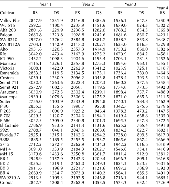
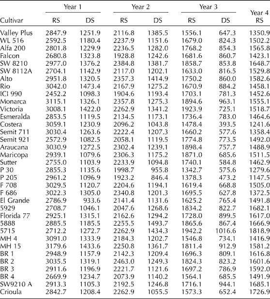
The results of DMY (kg/ha) per harvest for each cultivar during the RS and DS for each agricultural year are shown in Table 1. The average of DMY considering all cultivars and all harvests was 1979 kg/ha per harvest for RS and 1105 kg/ha per harvest for DS. The highest average DMY was observed for RS, as was expected, and was responsible for about 81.3–85.0% of annual DMY. The total annual DMY varied from 12,900 kg/ha (P205 cultivar) to 16,200 kg/ha (Monarca); from 10,900 kg/ha (P205) to 13,400 kg/ha (Monarca and BR 2) for RS and from 1900 kg/ha (P205) to 2900 kg/ha (SW 8210, Rio, 5715 and MH 15) for DS. Unequal seasonal DMY distribution could be observed for all cultivars. However, special attention is necessary to select superior productive genotypes that have a better production distribution during the year. Thus, it is also important to study the trait seasonal DMY distribution to verify whether genetic variability exists among cultivars. A possible cause of the pronounced unequal seasonal distribution is the fact that there was no effective irrigation of the experimental area. Thus, the lack of water in the DS was probably a determinant factor contributing to the low DMY observed.
Dry matter yield production means (kg/ha) per harvest for each cultivar, considering rainy season (RS) and dry season (DS) of each agricultural year
High standard deviations were observed, mainly for RS. These high values are associated with high DMY at the beginning of the experiment and low DMY at the end of the experiment. For instance, DMY of cultivar MH 15 in a single harvest ranged from 5509 to 419 kg/ha in RS and from 2219 to 552 kg/ha in DS. These accentuated decreases in yields over the years indicate that a meticulous study of the persistence of the cultivars must be performed.
Covariance structure and statistical tests
Selection of covariance structure was based on goodness of fit for criteria AIC and SBC. The larger the value of AIC or SBC, the better the structure. For both criteria, the best structure was SP(POW) for RS and DS. REML failed to converge when analyses were performed with UN structure, probably because it requires estimation of a large number of variance and covariance parameters.
Covariance components and correlations between harvests were estimated at RS and DS using SP(POW) structure, which models the covariance between two measurements at times t 1 and t 2 (Littell et al., Reference Littell, Milliken, Stroup and Wolfinger1996) as follows:

where ρ is an autoregressive parameter, estimates were 0.9803 and 0.9554 for RS and DS, respectively, and σ2 is the residual variance; estimates are shown below. The covariance matrix is printed for experimental unit number 1. It indicates that it is the covariance submatrix for the repeated measures from cultivar 1 drawn from block 1. All the other subjects (cultivars i versus block j) are assumed to have the same covariance matrix.
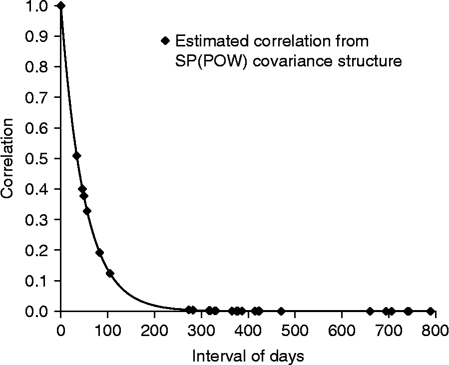
All correlations were of medium (for DS) and low (for RS) values or equal to zero (for RS and DS). It was also verified that there is no correlation between harvests when different agricultural years are compared. The most significant correlations were between adjacent harvests, which were illustrated for DS in Fig. 1. For RS, correlations between adjacent harvests at year 1 varied from 0.13 to 0.21; at year 2 varied from 0.00 to 0.25; at year 3 varied from 0.10 to 0.37; and at year 4 varied from 0.11 to 0.28. For DS, they were highest, ranging from 0.38 to 0.51 at year 1; from 0.33 to 0.38 at year 2 and equal to 0.40 at year 3. Thus, a linear association only appears between adjacent harvests in the same year, mainly at DS. It emphasizes the necessity to evaluate perennial alfalfa cultivars during different years and harvests.
Estimated correlations from SP(POW) covariance structure between harvests (expressed in interval of days) of alfalfa cultivars evaluated in dry season, showing the decay in correlation between harvests.

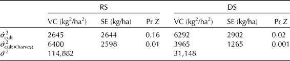
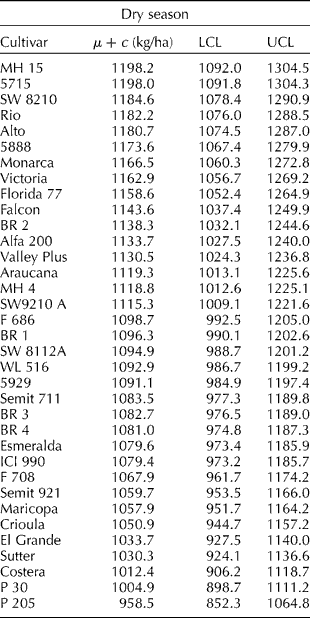
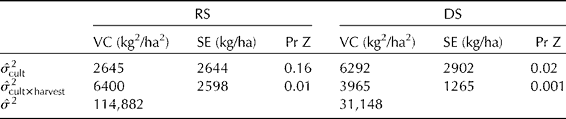
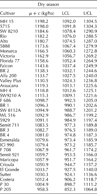
Variance components estimated by REML as well as the standard errors associated with each estimate and approximate Wald tests are in Table 2. The hypothesis  was only rejected at the 16% level of significance for RS and at the 2% level of significance for DS. This result indicates that genetic variability among cultivars is larger at DS. Thus, selection of superior cultivars will be more efficient if it is based on predicted genotypic values of cultivars in this season. The rank of 35 alfalfa cultivars, based on EBLUP of cultivar effect evaluated in DS considering the SP(POW) structure, is presented in Table 3. Upper and lower confidence limits for each cultivar are also shown in Table 3.
Cultivar  , interaction cultivar with harvest
 and residual
 variance component estimates (VC) obtained by REML, their standard errors (SE) and approximate Wald test (Pr Z) for rainy season (RS) and dry season (DS)
Rank of 35 alfalfa cultivars based on EBLUP of cultivar effect (μ+c) in kilograms (kg) per hectare (ha), lower confidence limit (LCL) and upper confidence limit (UCL) of confidence interval of the genotypic effect evaluated in dry season
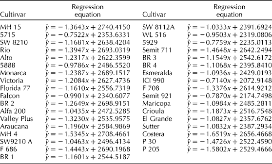
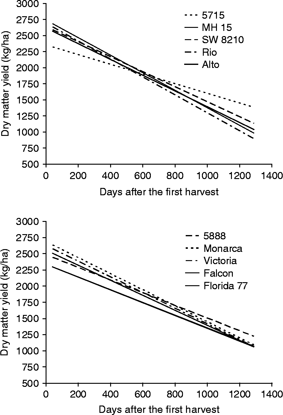
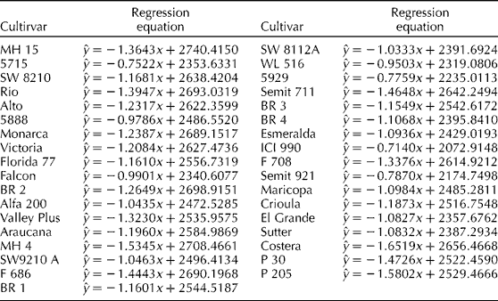
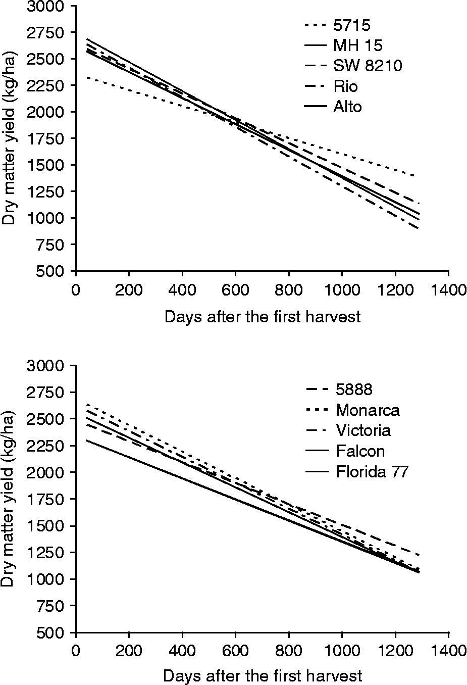
The hypothesis  was rejected at 1 and 0.1% level of significance for RS and DS, respectively (Table 2). It indicates that there is a significant interaction among cultivars and harvests. Simple linear regression of dry matter production (y) on days after the first harvest (x) has presented the best fit of the data, when comparing with the quadratic linear regression. The regression equations obtained are presented in Table 4. The productivity over the years of ten alfalfa cultivars selected in DS (Table 3) was studied from regression analyses considering all harvests and can be observed in Fig. 2.
Simple linear regression equations of dry matter production (y) on days after the first harvest (x), considering all harvests for 35 alfalfa cultivar evaluated at tropical environment
Productivity (dry matter yield – kg/ha) over the years (42–1288 days after the first harvest) of ten alfalfa cultivars selected in dry season from EBLUP, considering all harvests.
Discussion
Some experiments in Brazil have also shown the absence of genetic variability of alfalfa cultivars. Monteiro et al. (Reference Monteiro, Costa and Silveira1998) evaluated 17 alfalfa cultivars in a subtropical climate in Brazil and did not find significant differences among cultivars for annual dry matter production. The results obtained for dry matter production per harvest during summer and winter indicated significant differences only for the 1992 winter. The authors used the ANOVA and classified cultivars as fixed effects. On the other hand, several experiments carried out in Minas Gerais, Brazil, showed significant differences among alfalfa cultivars when DMY per harvest was the evaluated trait (Souza-Sobrinho et al., Reference Souza-Sobrinho, Ledo, Pereira, Botrel, Evangelista and Viana2004). These data were also analyzed using variances in a split plot design. Thus, genetic variability detection is influenced by the evaluated cultivars, the experimental precision, the genetic–environmental interaction and the statistical methodology used.
Approximate Wald test and standard errors are based on asymptotic properties and are not very reliable if the degrees of freedom to estimate the variance component are small (Littell et al., Reference Littell, Milliken, Stroup and Wolfinger1996; Steel et al., Reference Steel, Torrie and Dickey1997). Another approximate test is possible when a set of model parameters can be set to zero. This is called the likelihood ratio test, drawing from likelihood theory. It is computed taking the difference between the -2 REML log likelihood of the model containing the random effect, whose component will be tested, and the model without it. This difference is compared to a chi-square (χ2) distribution. The hypothesis  was only rejected at the 14% level of significance (χ2 = 1.2) for RS and at the 0.2% level of significance (χ2 = 8.2) for DS. The hypothesis
 was rejected at the 0.5% (χ2 = 6.8) and the 0.01% (χ2 = 13.6) levels of significance for RS and DS, respectively. These p-values were obtained by taking half of the probability of a greater χ2 from a χ2 distribution with one degree of freedom. It can be noted that likelihood ratio tests generated smaller p-values than Wald tests, but the discussion made above is still appropriate.
Since the hypothesis  was rejected, the classification of cultivars for RS and DS changes over different harvests. Consequently, the identification of the most productive cultivars depends on the evaluation during several harvests. It can be appropriately analyzed by a mixed model methodology using cultivars ranking based on EBLUP of genotypic values that consider all harvests to predict these effects.
Regression analyses were also performed to study the cultivars productivity over the years, since the interactions between cultivars and harvests were significant. According to a simple linear regression, it is important to verify: (a) the intercept value of the equation, which is related to the cultivar productivity; and (b) the angular coefficient, which is related to the persistence of the cultivar. Since all angular coefficients were negative (Table 4), the closer they are to zero the greater the persistence of cultivar. It is interesting to note that the cultivar 5715 showed a less pronounced reduction in dry matter production over the years, being a persistent and productive genotype in tropical regions (Fig. 2). Estimated DMY per harvest was 1385 kg/ha after 3.5 years of evaluation. On the other hand, cultivar MH 15 showed a sharper decrease in DMY, although its estimated production was 2883 kg/ha 42 days after the first harvest. Thus, observing the rank of alfalfa cultivars (Table 3) and the linear regression equations estimated (Table 4), it is possible to verify that the most productive cultivars are not always the more persistent.
The genetic variability was more expressive in DS; therefore, selection of superior genotypes based on DMY should consider EBLUP for this season. The first ten cultivars with higher genotypic values were: MH 15, 5715, SW 8210, Rio, Alto, 5888, Monarca, Victoria, Florida 77 and Falcon. Crioula, the most common cultivar in Brazil, showed low forage potential in Sertãozinho. Results demonstrate that more productive alfalfa cultivars can be used in tropical pastures.
The use of multiple comparison tests is not appropriate when the number of treatments is greater than four, since they have low capacity to detect significant differences (Steel et al., Reference Steel, Torrie and Dickey1997; Resende and Duarte, Reference Resende and Duarte2007). Moreover, treatments should be treated as random effects. Thus, lower and upper confidence limits of the genotypic effects were calculated for each cultivar. Confidence limits are the lower and upper boundaries of a confidence interval, i.e. the values that define the range of a confidence interval (Snedecor and Cochran, Reference Snedecor and Cochran1989). The interval estimate gives an indication of how much uncertainty there is in the estimate of the true parameter. The narrower the interval is, the more precise the estimate.
This statistical approach, based on a mixed model methodology, has proven to be an interesting way to analyze data from perennial herbage-breeding programmes. It allows testing and selecting of appropriate covariance structure within cultivars and among harvests and also indicates superior cultivars that can be selected by cultivar effects of EBLUP. Moreover, it allows for analysis of the possible interactions between cultivars and harvests. Correlations between harvests were estimated, providing a better understanding of the relationship between production and the harvests during different seasons of the year.
Acknowledgements
The authors acknowledge the Fundação de Amparo à Pesquisa do Estado de São Paulo (FAPESP) for the financial support.