1 Introduction
Strong departures from Gaussianity are a hallmark feature of fully developed turbulence. The probability density functions (PDFs) of small-scale quantities measured in turbulent flows, such as the gradients of velocity fields or particle accelerations, display heavy tails with comparably large probabilities of encountering extreme events many times larger than the corresponding standard deviation. The frequent occurrence of extreme acceleration events has broad implications – for instance, it directly impacts droplet collision rates and therefore the droplet size distributions in a cloud (Shaw Reference Shaw2003).
The strongly non-Gaussian statistics of particle accelerations is the cause of Lagrangian small-scale intermittency: for large time lags the Lagrangian velocity increment PDF is almost Gaussian as a result of the nearly Gaussian single-point statistics of the velocity, but as the time lag is reduced, the Lagrangian velocity increment becomes proportional to the particle acceleration, therefore the statistics become more and more non-Gaussian, with a heavy-tailed PDF. Direct experimental measurements of Lagrangian tracer statistics were pioneered by Snyder & Lumley (Reference Snyder and Lumley1971), with significant progress being further made, for example, by Sato & Yamamoto (Reference Sato and Yamamoto1987), Virant & Dracos (Reference Virant and Dracos1997), Voth, Satyanarayan & Bodenschatz (Reference Voth, Satyanarayan and Bodenschatz1998), Ott & Mann (Reference Ott and Mann2000), La Porta et al. (Reference La Porta, Voth, Crawford, Alexander and Bodenschatz2001), Lehmann, Nobach & Tropea (Reference Lehmann, Nobach and Tropea2002), Voth et al. (Reference Voth, La Porta, Crawford, Alexander and Bodenschatz2002), Mordant, Levêque & Pinton (Reference Mordant, Levêque and Pinton2004), Reynolds et al. (Reference Reynolds, Mordant, Crawford and Bodenschatz2005), Volk et al. (Reference Volk, Mordant, Verhille and Pinton2008b ) and Xu & Bodenschatz (Reference Xu and Bodenschatz2008); numerical studies were first reported in Yeung & Pope (Reference Yeung and Pope1989), and continued, for example, by Vedula & Yeung (Reference Vedula and Yeung1999), Sawford et al. (Reference Sawford, Yeung, Borgas, Vedula, La Porta, Crawford and Bodenschatz2003) and Toschi et al. (Reference Toschi, Biferale, Boffetta, Celani, Devenish and Lanotte2005) with Reynolds numbers comparable to the experiments attained only recently (Sawford & Yeung Reference Sawford and Yeung2015). See also the review by Toschi & Bodenschatz (Reference Toschi and Bodenschatz2009) for a more comprehensive overview.
Lagrangian intermittency is closely related to its Eulerian counterpart: spatial velocity increment PDFs also change from slightly sub-Gaussian for large increments to heavy-tailed for small increments on the order of the Kolmogorov length scale. Bridging relations were established to connect Lagrangian to Eulerian statistics in previous works – for example, in the multifractal framework (Chevillard et al. Reference Chevillard, Roux, Levêque, Mordant, Pinton and Arneodo2003; Biferale et al. Reference Biferale, Boffetta, Celani, Devenish, Lanotte and Toschi2004; Buzzicotti et al. Reference Buzzicotti, Bhatnagar, Biferale, Lanotte and Ray2016) or in terms of PDF equations (Homann et al. Reference Homann, Kamps, Friedrich and Grauer2009; Kamps, Friedrich & Grauer Reference Kamps, Friedrich and Grauer2009; Lalescu & Wilczek Reference Lalescu and Wilczek2018) – revealing the repercussions of the spatial structure of turbulence on Lagrangian particle statistics.
The aim of the current paper is to further investigate the relation between Lagrangian and Eulerian statistics. Focusing on Lagrangian small-scale intermittency, our goal is to quantify the impact of Eulerian scales on Lagrangian acceleration statistics. Our findings may have implications for large eddy simulations (LES) of particulate flows, in which the influence of the unresolved scales need to be quantified (Zhou, Chen & Jin Reference Zhou, Chen and Jin2017) or modelled (see, for example, Mazzitelli, Toschi & Lanotte Reference Mazzitelli, Toschi and Lanotte2014). Our results also help to better understand the impact of the fine-scale structure of turbulence on finite-sized, neutrally buoyant particles in turbulence, which have been broadly investigated, for example, by Qureshi et al. (Reference Qureshi, Bourgoin, Baudet, Cartellier and Gagne2007), Volk et al. (Reference Volk, Calzavarini, Verhille, Lohse, Mordant, Pinton and Toschi2008a ), Xu & Bodenschatz (Reference Xu and Bodenschatz2008), Brown, Warhaft & Voth (Reference Brown, Warhaft and Voth2009), Homann & Bec (Reference Homann and Bec2010), Naso & Prosperetti (Reference Naso and Prosperetti2010), Volk et al. (Reference Volk, Calzavarini, Lévêque and Pinton2011), Cisse, Homann & Bec (Reference Cisse, Homann and Bec2013), Klein et al. (Reference Klein, Gibert, Bérut and Bodenschatz2013), Cisse et al. (Reference Cisse, Saw, Gibert, Bodenschatz and Bec2015) and Uhlmann & Chouippe (Reference Uhlmann and Chouippe2017). It has been argued by Voth et al. (Reference Voth, La Porta, Crawford, Alexander and Bodenschatz2002) that acceleration statistics can be estimated by considering only turbulent fluctuations at scales larger than the particle size, leading to an effective filtering. In fact, Calzavarini et al. (Reference Calzavarini, Volk, Bourgoin, Lévêque, Pinton and Toschi2009) employ filtering techniques to evaluate Faxén corrections in a simple numerical model of finite-sized particles. Qureshi et al. (Reference Qureshi, Bourgoin, Baudet, Cartellier and Gagne2007), Brown et al. (Reference Brown, Warhaft and Voth2009) and Volk et al. (Reference Volk, Calzavarini, Lévêque and Pinton2011) presented acceleration measurements from experiments with large, neutrally buoyant particles, focusing on PDFs and acceleration variances as they change with particle size. Notably, Volk et al. (Reference Volk, Calzavarini, Lévêque and Pinton2011) also discussed estimates of the acceleration flatness as a function of particle size. The experiments indicate scaling of the acceleration moments as a function of particle size, and the scaling laws are consistent with the view that only fluctuations of scales larger than the particle size contribute to their acceleration.
Here, we investigate acceleration statistics of Lagrangian tracers in filtered velocity fields by combining extensive direct numerical simulations (DNS) of homogeneous isotropic turbulence with spatial filtering. This numerical experiment is aimed at cleanly isolating the role of spatial scales – particle boundary layer effects, fluid-mediated interactions with other particles, as well as particle backreactions on the flow are deliberately neglected. By systematically eliminating scales, we are able to precisely quantify the impact of the spatial scales on Lagrangian acceleration statistics, and in particular on the occurrence of extreme events. As intuitively expected, we find that removing spatial scales systematically reduces the frequency of occurrence of extreme acceleration events. We show that this simple approach is sufficient to capture experimental results of acceleration variance and flatness of neutrally buoyant, finite-sized particles as a function of particle size. We furthermore test the robustness of the results with respect to the filtering procedure by comparing top-hat, Gaussian and sharp Fourier filters – i.e. we use filters that either have finite support in real space, are fast decaying in both real and Fourier space, or have finite support in Fourier space.
2 Lagrangian particles in filtered fields
In the following, we are considering an incompressible Navier–Stokes flow with a velocity field
 $\boldsymbol{u}$
. To systematically remove spatial scales from the flow, we employ filtering (see, for example, Germano Reference Germano1992), i.e. the velocity field is convolved with a filter kernel
 $\unicode[STIX]{x1D719}_{\ell }$
 $$\begin{eqnarray}\boldsymbol{u}_{\ell }(\boldsymbol{x},t)=\int \,\text{d}^{3}\boldsymbol{r}\,\boldsymbol{u}(\boldsymbol{r},t)\unicode[STIX]{x1D719}_{\ell }(\boldsymbol{x}-\boldsymbol{r}).\end{eqnarray}$$
The equations for the tracers of the filtered field,
 $$\begin{eqnarray}\frac{\text{d}}{\text{d}t}\boldsymbol{X}_{\ell }(\boldsymbol{x},t)=\boldsymbol{u}_{\ell }(\boldsymbol{X}_{\ell }(\boldsymbol{x},t),t),\quad \boldsymbol{X}_{\ell }(\boldsymbol{x},t_{0})=\boldsymbol{x}_{0},\end{eqnarray}$$
can then be used to compute trajectories of virtual particles that are affected only by fluctuations of characteristic scales larger than
 $\ell$
. For
 $\ell =0$
these equations reduce to the standard equations of motion for tracer particles. The acceleration of fluid particles can be obtained from the left-hand side of the Navier–Stokes equations. The acceleration of tracer particles in a filtered field obeys an analogous equation:
 $$\begin{eqnarray}\tilde{\boldsymbol{a}}_{\ell }(\boldsymbol{x},t)=[(\unicode[STIX]{x2202}_{t}+\boldsymbol{u}_{\ell }\boldsymbol{\cdot }\unicode[STIX]{x1D735})\boldsymbol{u}_{\ell }](\boldsymbol{x},t).\end{eqnarray}$$
As a subtle point, we note that this differs from the filtered acceleration
 $\boldsymbol{a}_{\ell }$
by the divergence of the subgrid-scale stress tensor,
 $\boldsymbol{a}_{\ell }=\tilde{\boldsymbol{a}}_{\ell }+\unicode[STIX]{x1D735}\boldsymbol{\cdot }\boldsymbol{{\mathcal{T}}}_{\ell }$
with
 $\boldsymbol{{\mathcal{T}}}_{\ell }\equiv (\boldsymbol{u}\boldsymbol{u})_{\ell }-\boldsymbol{u}_{\ell }\boldsymbol{u}_{\ell }$
. Experimentally, finite-sized particles are subject to a coarse-grained force, i.e.
 $\boldsymbol{a}_{\ell }$
in the simplest approximation (Voth et al.
Reference Voth, La Porta, Crawford, Alexander and Bodenschatz2002). We focus on
 $\tilde{\boldsymbol{a}}_{\ell }$
in our presentation, which, as detailed below, shows scaling properties consistent with
 $\boldsymbol{a}_{\ell }$
.
For studying the statistics of
 $\tilde{\boldsymbol{a}}_{\ell }$
, we use DNS – a standard pseudo-spectral solver for the Navier–Stokes equations in the vorticity formulation with a third-order Runge–Kutta method for time-stepping and a high-order Fourier smoothing (Hou & Li Reference Hou and Li2007) to reduce aliasing errors. A quasi-stationary regime was maintained by the use of a large-scale Lundgren type of forcing (Lundgren Reference Lundgren2003), active in a band of small wavenumbers
 $k\in [1.5,3]$
(DNS units). We consider three datasets first studied in Lalescu & Wilczek (Reference Lalescu and Wilczek2018), with Reynolds numbers based on the Taylor scale
 $R_{\unicode[STIX]{x1D706}}=208$
, 304, 429 and respective resolutions
 $k_{max}\unicode[STIX]{x1D702}=1.7$
, 1.4, 1.2 (here
 $k_{max}$
is the maximum wavenumber resolved by our DNS and
 $\unicode[STIX]{x1D702}$
is the Kolmogorov length scale). The simulations are computed on grids of respective sizes
 $1024^{3}$
,
 $1536^{3}$
,
 $2048^{3}$
, in the three-dimensional periodic domain
 $[0,2\unicode[STIX]{x03C0}]\times [0,2\unicode[STIX]{x03C0}]\times [0,2\unicode[STIX]{x03C0}]$
(DNS units). Fully developed turbulence with scale separations
 $L/\unicode[STIX]{x1D702}=168$
, 297, 468 and
 $T/\unicode[STIX]{x1D70F}_{\unicode[STIX]{x1D702}}=22.9$
, 33.5, 44.4 is achieved; here
 $L=\unicode[STIX]{x03C0}\int \,\text{d}k\,E(k)/(2k{u_{rms}}^{2})$
is the integral length,
 $T=L/u_{rms}$
is the Eulerian integral time, where
 $u_{rms}$
is the root-mean-squared velocity component, and
 $\unicode[STIX]{x1D70F}_{\unicode[STIX]{x1D702}}$
is the Kolmogorov time scale. The relevant statistics (for example, moments of acceleration components
 $\tilde{a}_{\ell }$
) are then computed in postprocessing, using regularly timed snapshots over intervals of 14, 6.1 and 4.4 Eulerian integral times, respectively.
In this study, we use three different types of filter to test the robustness of the results with respect to the choice of filters. We consider three spherically symmetric filters:
 $$\begin{eqnarray}\displaystyle & \displaystyle \unicode[STIX]{x1D719}_{\ell }^{b}(r)=\frac{1}{\ell ^{3}}\frac{6}{\unicode[STIX]{x03C0}}H(\ell /2-r) & \displaystyle\end{eqnarray}$$
 $$\begin{eqnarray}\displaystyle & \displaystyle \unicode[STIX]{x1D719}_{\ell }^{g}(r)=\frac{1}{\unicode[STIX]{x1D70E}_{\ell }^{3}}\frac{1}{(2\unicode[STIX]{x03C0})^{3/2}}\exp \left(-\frac{1}{2}\left(\frac{r}{\unicode[STIX]{x1D70E}_{\ell }}\right)^{2}\right) & \displaystyle\end{eqnarray}$$
 $$\begin{eqnarray}\displaystyle & \displaystyle \unicode[STIX]{x1D719}_{\ell }^{s}(r)=\frac{1}{2\unicode[STIX]{x03C0}^{2}r^{3}}(\sin k_{\ell }r-k_{\ell }r\cos k_{\ell }r), & \displaystyle\end{eqnarray}$$
where
 $H$
is the Heaviside step function.
 $\unicode[STIX]{x1D719}^{b}$
is a function that is constant inside the ball of radius
 $\ell /2$
;
 $\unicode[STIX]{x1D719}^{g}$
is a Gaussian filter with width
 $\unicode[STIX]{x1D70E}_{\ell }$
; and
 $\unicode[STIX]{x1D719}^{s}$
is the Fourier transform of a sharp Fourier low-pass filter at wavenumber
 $k_{\ell }$
. To compare the results obtained with different filters, we calibrate them by requesting that the field
 $\boldsymbol{u}_{\ell }$
has approximately the same energy, independently of the filter type used. Given the energy spectrum
 $E(k)$
, we require that
 $$\begin{eqnarray}\int _{0}^{\infty }\,\text{d}k\,E(k)\hat{\unicode[STIX]{x1D719}_{\ell }^{b}}(k)^{2}\approx \int _{0}^{\infty }\,\text{d}k\,E(k)\hat{\unicode[STIX]{x1D719}_{\ell }^{g}}(k)^{2}\approx \int _{0}^{\infty }\,\text{d}k\,E(k)\hat{\unicode[STIX]{x1D719}_{\ell }^{s}}(k)^{2},\end{eqnarray}$$
with
 $\unicode[STIX]{x1D719}^{b}$
chosen as a reference; the hat here indicates Fourier transforms. We find that using
 $\unicode[STIX]{x1D70E}_{\ell }=0.23\ell$
and
 $k_{\ell }=2.8/\ell$
leads to the three coarse-grained fields having the same energy in very good approximation. We note that Calzavarini et al. (Reference Calzavarini, Volk, Bourgoin, Lévêque, Pinton and Toschi2009) obtained Faxén corrections by calibrating a Gaussian filter to approximate spherical volume and surface integrals of the velocity, with a calibration factor of
 $1/(2\sqrt{5})$
, close to our 0.23.
3 Acceleration statistics
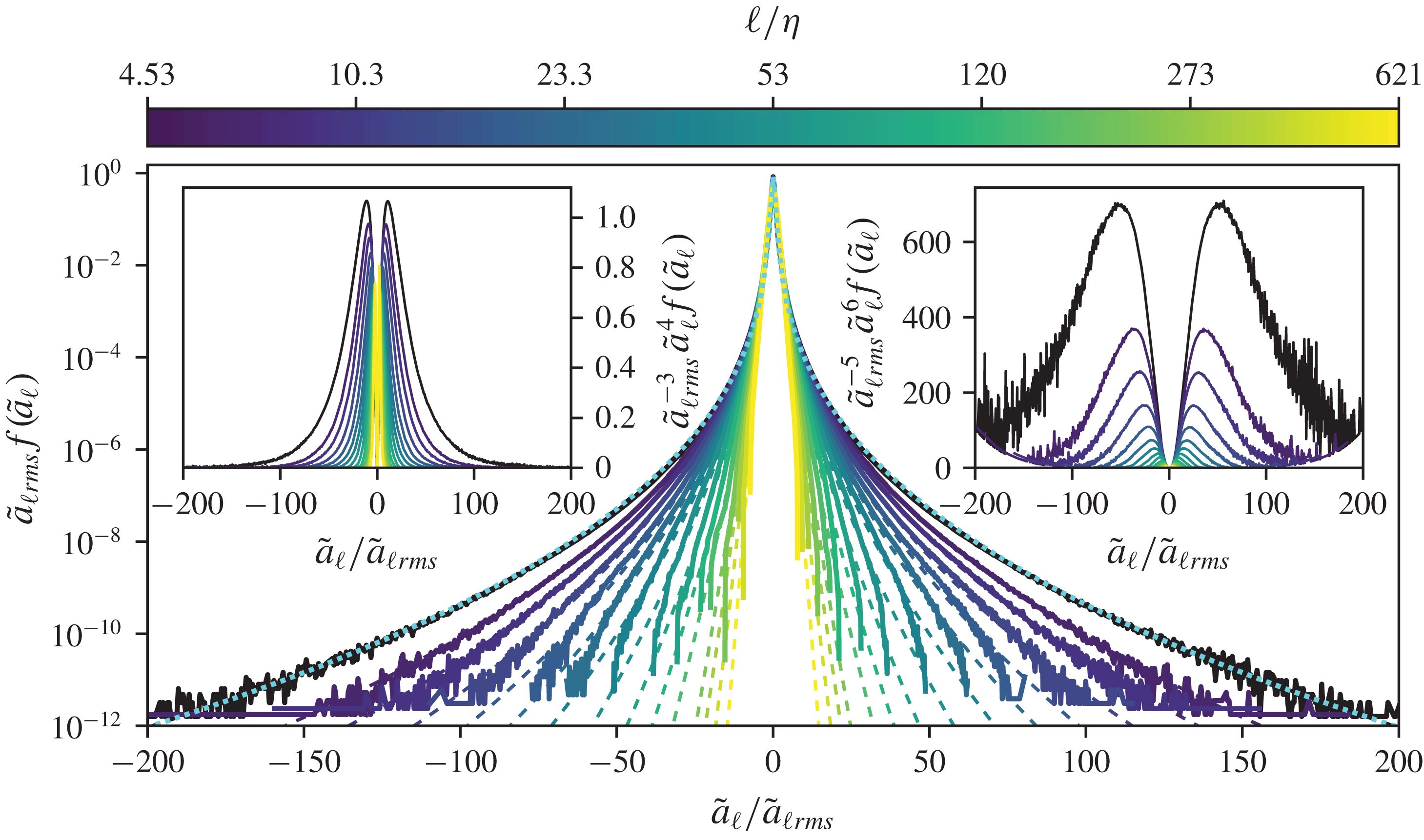
To provide the best possible statistical convergence, we compute the acceleration statistics directly from our extensive database of turbulent fields rather than from particle data. The resulting acceleration PDFs are presented in figure 1. The black curve corresponds to the acceleration PDF of regular fluid particles at
 $R_{\unicode[STIX]{x1D706}}=429$
. In agreement with previous works (La Porta et al.
Reference La Porta, Voth, Crawford, Alexander and Bodenschatz2001; Sawford et al.
Reference Sawford, Yeung, Borgas, Vedula, La Porta, Crawford and Bodenschatz2003; Ishihara et al.
Reference Ishihara, Kaneda, Yokokawa, Itakura and Uno2007; Volk et al.
Reference Volk, Calzavarini, Lévêque and Pinton2011), the PDF is pronouncedly heavy-tailed, extending to accelerations 200 times larger than the root-mean-squared acceleration
 $a_{rms}$
in our dataset. For reference, the dotted (cyan) line shows the stretched exponential fit introduced in La Porta et al. (Reference La Porta, Voth, Crawford, Alexander and Bodenschatz2001):
 $f(a)=C\exp (-(a/\unicode[STIX]{x1D70E})^{2}/(1+|\unicode[STIX]{x1D6FD}a/\unicode[STIX]{x1D70E}|^{\unicode[STIX]{x1D6FE}}))$
with
 $\unicode[STIX]{x1D6FD}=0.4981$
,
 $\unicode[STIX]{x1D70E}=0.5073a_{rms}$
and
 $\unicode[STIX]{x1D6FE}=1.636$
for the unfiltered acceleration. In fact, the same formula can be used to also fit acceleration PDFs of tracers of filtered fields (see thin, dashed lines). Compared to the acceleration PDF tails of regular tracers, those of tracers of filtered fields are reduced with increasing filter size. This can be explained by the fact that the acceleration field, comprised of the pressure gradient and viscous Laplacian fields, exhibits a pronounced fine-scale structure which is smoothed out by the filtering. Furthermore, large acceleration events have been related to trapping events in small-scale vortices – for example, by Toschi et al. (Reference Toschi, Biferale, Boffetta, Celani, Devenish and Lanotte2005). Such events are also reduced by filtering, resulting in less heavy-tailed statistics. We note, however, that the PDF does not become Gaussian for increasing
 $\ell$
: the tails follow a stretched exponential form for a range of scales. A steeper drop-off towards extreme accelerations (not captured by the formula) is observed for larger
 $\ell$
, but the parametrization is quite accurate for the majority of the PDFs’ support.
Tracer acceleration PDFs, computed from the filtered velocity field for the
 $R_{\unicode[STIX]{x1D706}}=429$
DNS. Thin, dashed lines in the background are individual stretched exponential fits with the formula introduced in La Porta et al. (Reference La Porta, Voth, Crawford, Alexander and Bodenschatz2001) (see text for details). The two insets show linear plots of the PDFs premultiplied with the fourth and sixth power of the acceleration: the fourth-order moment is well converged, and the sixth-order moment is well converged for
 $\ell \geqslant 4.53$
.

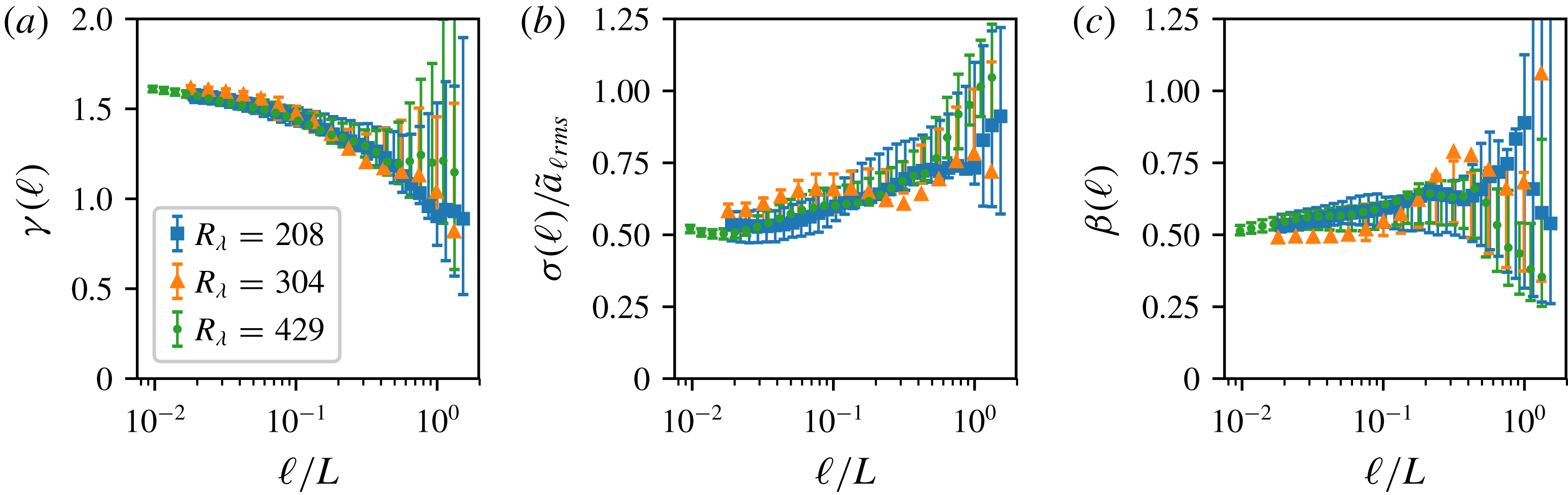
Fit parameters for the stretched exponential fits as a function of filter scale for three DNS. Errors are estimated through bootstrapping (see text for details). (a) Fitted stretching exponent
 $\unicode[STIX]{x1D6FE}(\ell )$
. (b) Fitted
 $\unicode[STIX]{x1D70E}(\ell )$
, normalized by the corresponding root-mean-squared acceleration. (c) Fitted
 $\unicode[STIX]{x1D6FD}(\ell )$
.

Figure 2 shows how the parameters of the stretched exponential fits change as the filter scale
 $\ell$
is increased. Errors are estimated with bootstrapping: PDFs of individual field snapshots are fitted independently, and 80 % of the corresponding values are contained in the intervals displayed as error bars. Symbols denote the parameters obtained for the fit of the time-averaged PDF. As the large scales converge only slowly in time, the errors are quite large for
 $\ell \geqslant L/2$
. One observation stands out: within errors, the parameters are independent of
 $R_{\unicode[STIX]{x1D706}}$
when the filter length is considered as a fraction of
 $L$
. This is consistent with the intuitive interpretation that filtering a turbulent flow effectively leads to a smaller
 $R_{\unicode[STIX]{x1D706}}$
, determined by the filter scale. In fact, given the energy spectrum of the filtered field
 $E(k)\hat{\unicode[STIX]{x1D719}}_{\ell }(k)^{2}$
, and the energy injection rate
 $\unicode[STIX]{x1D700}$
(which is on average equal to the energy transfer rate and the dissipation rate for large
 $R_{\unicode[STIX]{x1D706}}$
), one may compute the corresponding effective viscosity
 $\unicode[STIX]{x1D708}^{(\ell )}=\unicode[STIX]{x1D700}/\int _{0}^{\infty }\,\text{d}k\,k^{2}E(k)\hat{\unicode[STIX]{x1D719}}_{\ell }(k)^{2}$
, as well as effective statistical quantities such as the root-mean-squared velocity
 $u_{rms}^{(\ell )}$
, the effective Taylor microscale
 $\unicode[STIX]{x1D706}^{(\ell )}={u_{rms}}^{(\ell )}\sqrt{15\unicode[STIX]{x1D708}^{(\ell )}/\unicode[STIX]{x1D700}}$
, and therefore an effective
 $R_{\unicode[STIX]{x1D706}}^{(\ell )}={u_{rms}}^{(\ell )}\unicode[STIX]{x1D706}^{(\ell )}/\unicode[STIX]{x1D708}^{(\ell )}$
. Assuming
 $E(k)$
is the typical energy spectrum of a high-
 $R_{\unicode[STIX]{x1D706}}$
flow, and that
 $\ell$
is in the inertial range, it follows that
 $R_{\unicode[STIX]{x1D706}}^{(\ell )}$
is independent of
 $R_{\unicode[STIX]{x1D706}}$
. Our fitting results show that the PDFs of accelerations of coarse-grained field tracers are essentially characterized by
 $R_{\unicode[STIX]{x1D706}}^{(\ell )}$
.
The well-resolved PDFs imply that our data have well-resolved fourth- and sixth-order statistics. The insets of figure 1 show premultiplied PDFs: integrating the curves yields the fourth- and the sixth-order moment, respectively. Here, we would like to emphasize that the computed fourth-order moments are statistically well converged, and the errors made for the sixth-order moment are small for
 $\ell >0$
. For fluid particles,
 $\tilde{a}_{\ell }^{6}f(\tilde{a}_{\ell })$
only decreases to about 10 % of its maximum value at the outermost bins used in our histograms; however, once filtering is applied, we note that a much better estimate of the area under the curve can be obtained, improving more and more with increasing
 $\ell$
. In the following, we discuss observed scaling of normalized acceleration moments for
 $\ell \gtrsim 10\unicode[STIX]{x1D702}$
where the moments are indeed statistically converged.
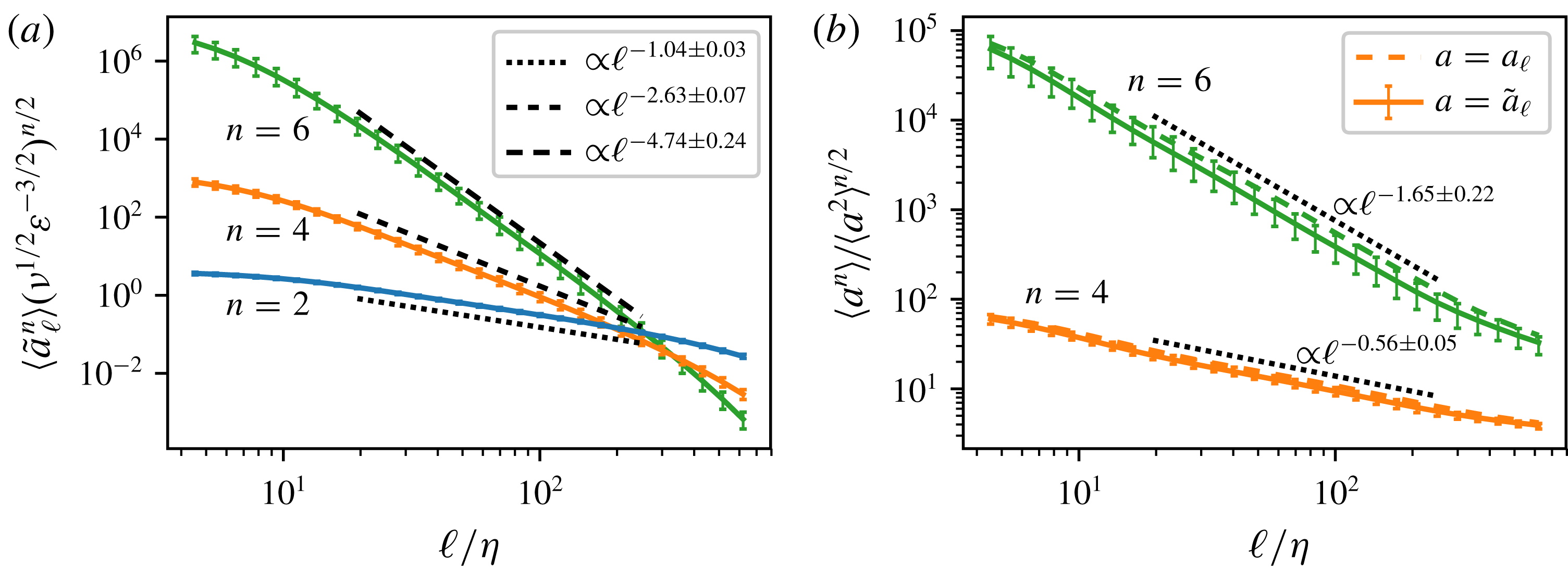
Moments of the acceleration as a function of filter scale for
 $R_{\unicode[STIX]{x1D706}}=429$
. Errors are estimated through bootstrapping (see text for details). (a) Second-, fourth- and sixth-order moments of the tracer acceleration (continuous lines). Scaling laws for the appropriate range are also shown, with the exponents obtained by least-squares fitting. (b) Scaling for normalized moments. Continuous lines designate tracer acceleration
 $\tilde{a}_{\ell }$
, dashed lines designate filtered acceleration
 $a_{\ell }$
– the distinction between moments of
 $a_{\ell }$
and
 $\tilde{a}_{\ell }$
is only noticeable for
 $n=4,6$
. Dotted lines show corresponding scaling laws. Errors for
 $a_{\ell }$
(which are comparable to those for
 $\tilde{a}_{\ell }$
) are not shown for clarity.

In figure 3 we show the acceleration moments for the
 $R_{\unicode[STIX]{x1D706}}=429$
dataset, using the Gaussian filter; the influence of filter choice on the results is discussed at the end of this section. A bootstrapping procedure is applied here as well: error bars designate intervals containing 80 % of the moments computed for individual field snapshots, while the symbols denote the time-averaged moment. Consistent with the trend observed in figure 1, the acceleration moments decrease as the filtering scale is increased and larger and larger fluctuations are removed from the velocity field. Both moments of
 $a_{\ell }$
and
 $\tilde{a}_{\ell }$
show scaling ranges with non-trivial scaling exponents, which depart from the Kolmogorov 1941 (K41) predictions
 $\langle a_{\ell }^{n}\rangle \sim (\ell /L)^{-n/3}$
(discussed later in this section). Regarding the difference between the statistics of tracers of filtered fields and the statistics of filtered acceleration fields, figure 3(b) shows that the differences in magnitude between
 $a_{\ell }$
and
 $\tilde{a}_{\ell }$
are significant for high-order moments. The measured scaling exponents themselves, however, which are important for the following discussion, are identical to within 3 %; a theoretical argument to this effect is given below.
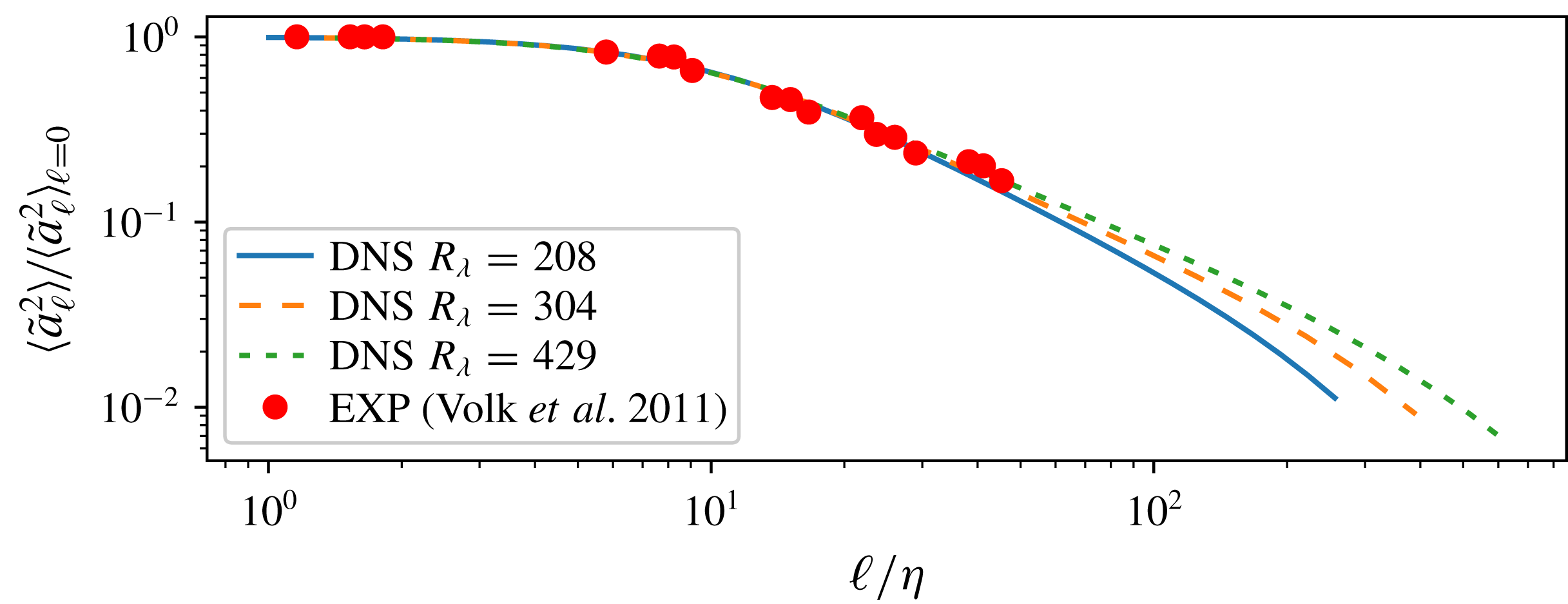
Tracer acceleration variance as a function of filter scale for different DNS (continuous lines), compared with experimental results of neutrally buoyant particles of sizes
 $D=\ell$
from Volk et al. (Reference Volk, Calzavarini, Lévêque and Pinton2011) (symbols).

We now compare our results with previous experimental results, in which the acceleration statistics of finite-sized, neutrally buoyant particles was addressed in terms of filtered acceleration fields. In the previous experimental works (Voth et al.
Reference Voth, La Porta, Crawford, Alexander and Bodenschatz2002; Qureshi et al.
Reference Qureshi, Bourgoin, Baudet, Cartellier and Gagne2007; Brown et al.
Reference Brown, Warhaft and Voth2009) the available data only allowed estimating the PDF over the comparably narrow interval
 $\tilde{a}\in [-15\tilde{a}_{\ell rms},15\tilde{a}_{\ell rms}]$
. Considering only this range of accelerations for
 $\ell \leqslant 50\unicode[STIX]{x1D702}$
, we indeed find that the cores of the PDFs are quite close, consistent with the experimental works. A direct comparison with the experimental results of Volk et al. (Reference Volk, Calzavarini, Lévêque and Pinton2011) (
 $590\leqslant R_{\unicode[STIX]{x1D706}}\leqslant 1050$
) is made in figure 4. The tracer acceleration variance is normalized by the fluid particle acceleration variance, in order to collapse the varying
 $R_{\unicode[STIX]{x1D706}}$
data in the dissipation range. The experimental data show a surprisingly good overall agreement with our DNS data: for very small particle diameters the acceleration variance is identical to that of fluid particles, then there is a transition to a scaling range at
 $\ell \approx 10\unicode[STIX]{x1D702}$
, for both the DNS and experimental datasets. For the DNS, the value of
 $\ell$
at which the transition occurs depends on the filter calibration; the agreement with the experiments gives, albeit a posteriori, a physical justification for choosing
 $\unicode[STIX]{x1D719}^{b}$
as the reference filter. In the inertial range we observe a slight
 $R_{\unicode[STIX]{x1D706}}$
dependency of our data, with differences between the three curves roughly comparable to differences from the experimental data. Volk et al. (Reference Volk, Calzavarini, Lévêque and Pinton2011) use two different fits of the acceleration PDF to give two estimates for the scaling exponent of the acceleration flatness,
 $-0.40$
and
 $-0.60$
, which are also roughly consistent with our numerical result of
 $-0.56$
. These results indicate that the scaling behaviour of acceleration moments of passive tracers of filtered fields is consistent with experimental results on finite-sized, neutrally buoyant particles, although the physics of the particle–flow interaction is significantly simpler in our numerical study.
Regarding theoretical arguments for our observations, predictions on filtered acceleration statistics can be made starting from the filtered Navier–Stokes equations, discussed in detail in Germano (Reference Germano1992). In Qureshi et al. (Reference Qureshi, Bourgoin, Baudet, Cartellier and Gagne2007) large, neutrally buoyant particles are studied, and it is argued that the force acting on these particles is, in essence, the pressure gradient filtered at the scale of the particle. This in turn leads to the prediction
 $\langle a_{\ell }^{2}\rangle \sim \ell ^{-2}S_{2}^{p}(\ell )$
, where
 $S_{n}^{p}$
is the
 $n$
th-order structure function of the pressure. The argument can be straightforwardly extended to general
 $n$
, showing that
 $\langle a_{\ell }^{n}\rangle \lesssim \ell ^{-n}S_{n}^{p}(\ell )$
, by using the triangle inequality for
 ${\mathcal{L}}^{n}$
norms, and assuming that the forcing term is independent of
 $\ell$
and that
 $\ell \ll L$
. The simple K41 prediction mentioned above is obtained by assuming
 $S_{n}^{p}(\ell )\sim (\ell /L)^{2n/3}$
.
Velocity (a) and pressure (b) structure functions (continuous lines) for DNS data at
 $R_{\unicode[STIX]{x1D706}}=429$
. Scaling exponents are estimated by a least-squares fit in the approximate range
 $30\unicode[STIX]{x1D702}<\ell <L$
, and the corresponding power laws are shown with dotted and dashed lines. Error estimates are obtained by bootstrapping (see text for details). Insets show the corresponding logarithmic derivatives over the same
 $\ell$
range, with dotted thin lines (obtained from individual snapshots) shown to quantify uncertainty; dashed vertical lines are placed at
 $\ell =30\unicode[STIX]{x1D702}$
and
 $\ell =L$
for reference.

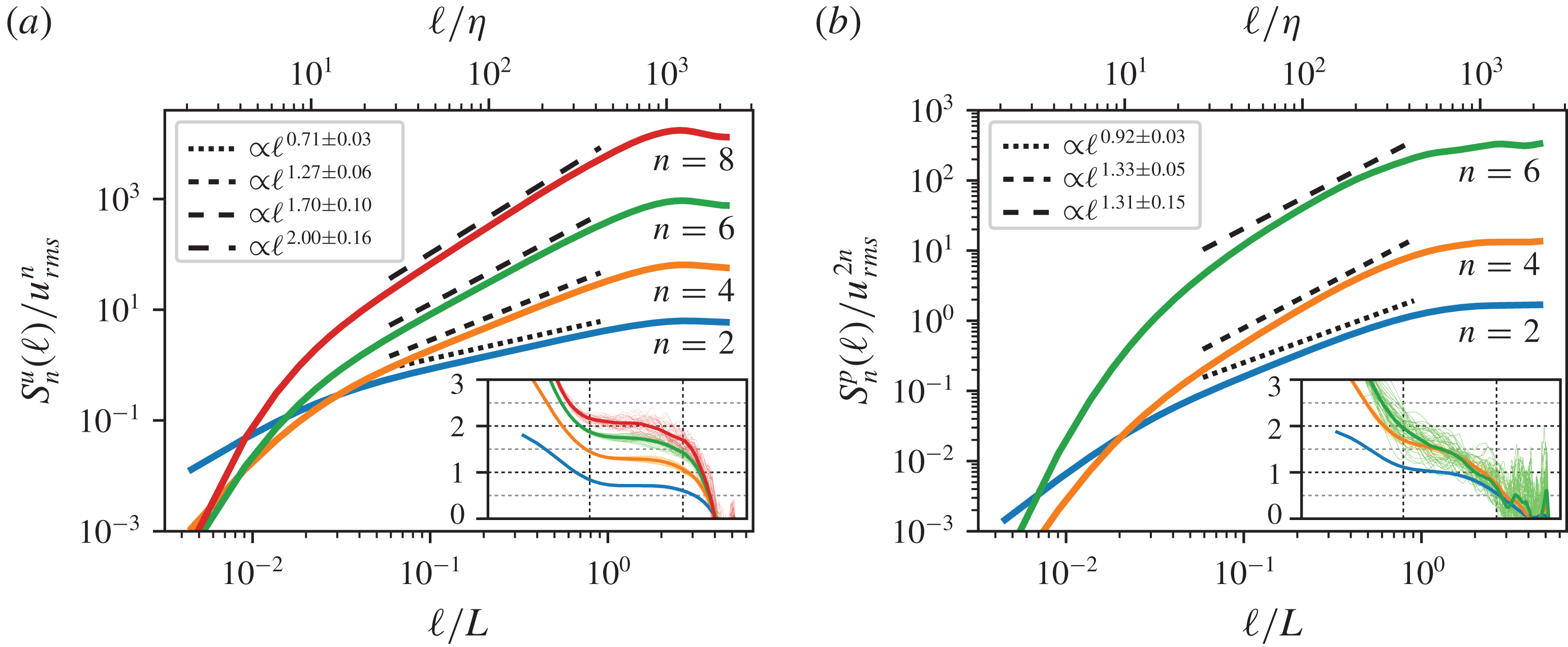
In figure 5 we show velocity and pressure structure functions (for the velocity we consider
 $S_{n}^{u}(\ell )\equiv \langle |\unicode[STIX]{x1D6FF}_{\ell }\boldsymbol{u}|^{n}\rangle$
). Panel (a) shows a clear scaling region for the velocity structure functions in the interval
 $30\unicode[STIX]{x1D702}\leqslant \ell \leqslant L$
(the scaling exponents are extracted with least-squares fitting, and the same bootstrapping procedure as above is used for error estimation). Assuming a pressure structure function scaling with exponents
 $\unicode[STIX]{x1D709}_{n}$
,
 $S_{n}^{p}(\ell )\lesssim (\ell /L)^{\unicode[STIX]{x1D709}_{n}}$
, we also use least-squares fitting over the same
 $30\unicode[STIX]{x1D702}\leqslant \ell \leqslant L$
range to obtain
 $\unicode[STIX]{x1D709}_{2}=0.92\pm 0.03$
,
 $\unicode[STIX]{x1D709}_{4}=1.33\pm 0.05$
and
 $\unicode[STIX]{x1D709}_{6}=1.31\pm 0.15$
for the
 $R_{\unicode[STIX]{x1D706}}=429$
dataset. Furthermore it can be shown that
 $\unicode[STIX]{x1D709}_{6}\geqslant \unicode[STIX]{x1D709}_{4}$
(Eyink Reference Eyink2007), which our data are consistent with when considering the errors. To better illustrate the limitations of the fitted scaling laws, the insets of figure 5 show logarithmic derivatives of the structure functions. We note that this approach gives even larger error estimates for
 $\unicode[STIX]{x1D709}_{4}$
and
 $\unicode[STIX]{x1D709}_{6}$
, when extracting the exponents from the same
 $\ell$
range. In the interest of avoiding unintentional biases when defining scaling exponents, we have chosen to use the same
 $\ell$
range for all fits, as well as the same bootstrapping technique for error estimation. The measurements lead to the predictions
 $-1.08$
,
 $-2.67$
and
 $-4.69$
for the corresponding acceleration moments, which agree with our observations (figure 3) to within 4 %. Also the corresponding predictions for the normalized moments,
 $-0.51$
and
 $-1.45$
, are quite close to the fit results. Because
 $\boldsymbol{{\mathcal{T}}}_{\ell }\sim S_{2n}^{u}(\ell )$
(Eyink Reference Eyink2007), it can be directly argued that
 $\langle \tilde{a}_{\ell }^{n}\rangle \sim (\ell /L)^{min[\unicode[STIX]{x1D709}_{n}-n,\unicode[STIX]{x1D701}_{2n}-n]}$
, where
 $\unicode[STIX]{x1D701}_{n}$
are the scaling exponents of the velocity (T. Drivas, 2018, Private communication). Since
 $\unicode[STIX]{x1D709}_{n}<\unicode[STIX]{x1D701}_{2n}$
, it is then only natural that both types of accelerations have the same scaling properties, as previously observed. The results are intriguing: even though the pressure structure functions do not show simple power-law scaling in the inertial range, the power laws extracted with a least-square fitting predict the correct scaling exponents of the acceleration moments, which do show scaling regions. We note that Volk et al. (Reference Volk, Calzavarini, Lévêque and Pinton2011) measured second- and fourth-order pressure structure functions in their experiment, obtaining
 $\unicode[STIX]{x1D709}_{2}=1.2\pm 0.1$
and
 $\unicode[STIX]{x1D709}_{4}-2\unicode[STIX]{x1D709}_{2}=-0.38\pm 0.03$
, different from our measurements. The discrepancy may originate in the measurement being performed, as the authors state, outside the bulk of the flow. Previously, second-order pressure structure functions and pressure spectra had been investigated experimentally by Pearson & Antonia (Reference Pearson and Antonia2001), Tsuji & Ishihara (Reference Tsuji, Ishihara and Kida2006), and numerically by Vedula & Yeung (Reference Vedula and Yeung1999), Gotoh & Fukayama (Reference Gotoh and Fukayama2001) and Ishihara et al. (Reference Ishihara, Kaneda, Yokokawa, Itakura and Uno2003): the scaling exponent of the pressure spectrum, in particular, is shown to reach a stationary value for
 $R_{\unicode[STIX]{x1D706}}$
at least of order 600. Therefore the differences may also be due to lingering small
 $R_{\unicode[STIX]{x1D706}}$
effects in our DNS.
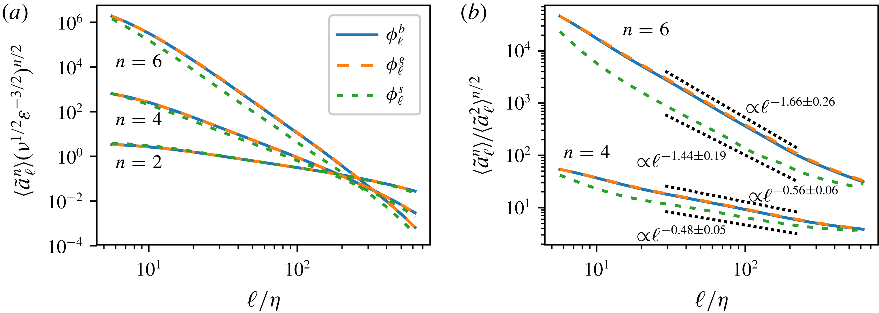
Before concluding, we briefly discuss the influence of the filter shape on the results. In figure 6(a) we show the moments of the tracer acceleration
 $\tilde{a}_{\ell }$
, as a function of the filter scale, obtained with the three different filters. Interestingly, the second-order moments collapse over the inertial range – even though the acceleration variance is a small-scale quantity and the filters are calibrated with a large-scale quantity. The sharp Fourier filter yields significantly different higher-order results than the other two filters; such deviations are not unexpected, since the sharp Fourier filter is the only one which is not positive-definite in its real-space representation, additionally to not being of finite support. These differences are further emphasized in panel (b) of the same figure, where we show the normalized fourth- and sixth-order moments. The results obtained with the positive-definite filters are, however, extremely close, with all the curves overlapping almost perfectly. We find that measured scaling exponents as well as the corresponding prefactors are quite robust to the choice of the two finite-support filters that we tested.
Influence of filter on acceleration statistics, for the
 $R_{\unicode[STIX]{x1D706}}=429$
case. Error bars are not shown for clarity, but they are consistent with those shown in figure 3. (a) Moments of the tracer acceleration versus filter scale. (b) Normalized moments of the tracer acceleration versus filter scale; dashed lines show power-law fits next to the relevant curves.

4 Conclusions
In this paper, we have studied the accelerations of passive tracers of the filtered velocity field based on direct numerical simulations of fully developed turbulence. In particular, we have analysed well-resolved PDFs and moments of order 2, 4 and 6. Our results indicate a scaling range of the acceleration moments as a function of filter scale, which can be explained based on pressure structure functions. As expected, filtering reduces the relative frequency of occurrence of extreme events. As a result, the standardized acceleration PDF tails become less heavy as the filter scale increases. Intuitively, extreme accelerations are associated with the small-scale structure of the velocity field; we observe that filtering out the small scales leads to acceleration moments decreasing as power laws of the filter length.
To directly test the common picture that spatial filtering is a dominant effect in the acceleration statistics of finite-sized, neutrally buoyant particles, we have compared our results to analytic predictions and experimental data. Indeed, we observe that low-order acceleration statistics of large, neutrally buoyant particles can be captured by tracers of filtered velocity fields: acceleration variances are reproduced quite well, and the acceleration flatness, while displaying a large margin of error for the experimental data, is also consistent. We also note that our numerical results on the acceleration variance are quite robust to the change of the filter shape, even though our filters range from one with finite support in Fourier space to one with finite support in real space.
However, our results show that the shape of the filter used in numerical approaches does influence high-order statistics of the filtered acceleration. In particular, when using a sharp Fourier cutoff, the acceleration flatness scales with an exponent of
 $-0.48$
, whereas when using a sharp real-space ball filter, or a Gaussian filter, the measured scaling exponent is
 $-0.56$
. These results are reminiscent of recent work by Buzzicotti et al. (Reference Buzzicotti, Linkmann, Aluie, Biferale, Brasseur and Meneveau2018), where it is shown that the energy transfer between scales displays different intermittency properties depending on the filter type.
The present study shows that tracers of the coarse-grained field reasonably approximate the acceleration statistics of finite-sized, neutrally buoyant particles. While the numerical modelling of realistic particles presents a significant challenge (see for instance the recent review by Maxey (Reference Maxey2017) and references therein), approaches like the one by Calzavarini et al. (Reference Calzavarini, Volk, Bourgoin, Lévêque, Pinton and Toschi2009) indicate that simple and efficient numerical models are sufficient to capture some features of finite-sized, neutrally buoyant particles. Our findings lend further support to this view. Our scaling results furthermore suggest that data from finite-sized particles can be used to extrapolate to smaller particles. This may also have implications on particle results from LES simulations. Here, the particle motion is only resolved on the cutoff scale of the LES. Using scaling results such as the one obtained here for the acceleration statistics, LES results could be extrapolated to unresolved scales to make statements about sub-resolution particle statistics.
Acknowledgements
We gratefully acknowledge helpful discussions with G. Voth, T. D. Drivas, N. Pujara and J. Lawson. We would also like to thank R. Volk for providing the data used in figure 4. Computations were performed on the clusters of the Max Planck Computing and Data Facility. Figures were generated with Matplotlib (Hunter Reference Hunter2007).