1 Introduction
In human blood, the haematocrit, that is, the volume fraction of red blood cells (RBCs), is usually between 40 % and 50 % while other cells, platelets and white blood cells, occupy less than 1 % of blood volume. Under healthy conditions, RBCs are highly deformable cells. This allows them to easily squeeze through narrow capillaries while preventing clogging even at high volume fraction, and to migrate away from vessel walls, which optimizes transport thanks to the formation of a lubricating cell-free layer. Cells also contribute strongly to blood viscosity and its shear-thinning behaviour (see Chien Reference Chien1970; Pries, Neuhaus & Gaehtgens Reference Pries, Neuhaus and Gaehtgens1992; Vitkova et al.
Reference Vitkova, Mader, Polack, Misbah and Podgorski2008; Fedosov et al.
Reference Fedosov, Pan, Caswell, Gompper and Karniadakis2011; Forsyth et al.
Reference Forsyth, Wan, Owrutsky, Abkarian and Stone2011), which allows for partial compensation for the higher heart power needed in situations of effort. While in most situations blood flow is influenced by interactions with walls and between cells, the question of the dynamics of a single RBC in a simple linear shear flow is of utmost fundamental interest and has been the subject of many experimental and theoretical studies owing to its complexity and its sensitivity to RBC properties. From a structural and mechanical viewpoint, an RBC is fundamentally a liquid drop encapsulated in a membrane. The cytosol is a haemoglobin solution with an average concentration (mean corpuscular haemoglobin concentration (MCHC)) normally between 320 and
 $360~\text{g}~\text{l}^{-1}$
corresponding to a mean viscosity in the range 6–10 mPa s (see Ross & Minton Reference Ross and Minton1977). The RBC membrane is composed of a lipid bilayer that provides area dilation resistance and bending rigidity, and a spectrin network that constitutes a quasi-2D skeleton on the inner surface of the lipid bilayer and connected to it via junction complexes and membrane proteins. This skeleton provides 2D shear elasticity to the membrane and to some extent shape memory. The cell volume is about
 $90~\unicode[STIX]{x03BC}\text{m}^{3}$
on average and the membrane area
 $136~\unicode[STIX]{x03BC}\text{m}^{2}$
, corresponding to a reduced volume of around 0.6 (see Linderkamp, Wu & Meiselman Reference Linderkamp, Wu and Meiselman1983; Fung Reference Fung1993). This leads to the characteristic biconcave disk shape and provides enough excess area (compared with a sphere) to allow large deformations.
Simple shear flow is a basic rheometric configuration and as such the dynamics of a suspended object can be considered as a marker of rheological and mechanical properties. In addition, it is also a benchmark situation for comparing experiments and theoretical or numerical modelling of the RBC. Indeed, there are still many open questions about the mechanical structure and properties of the RBC: what are the respective roles of the bending rigidity of the lipid bilayer, the elasticity of the spectrin network and the viscosity of the cytosol? Does the cytoskeleton have a permanent stress-free shape or should the possibility of remodelling be considered (e.g. due to nitric oxide (NO; see Grau et al. Reference Grau, Pauly, Ali, Walpurgis, Thevis, Bloch and Suhr2013; Simmonds, Detterich & Connes Reference Simmonds, Detterich and Connes2014) or adenosine triphosphate (ATP; see Betz et al. Reference Betz, Lenz, Joanny and Sykes2009) release and production in response to stress)? What is this stress-free shape (see Fischer et al. Reference Fischer, Haest, Stöhr-Liesen, Schmid-Schönbein and Skalak1981; Svelc & Svetina Reference Svelc and Svetina2012; Cordasco & Bagchi Reference Cordasco and Bagchi2014; Peng, Mashayekh & Zhu Reference Peng, Mashayekh and Zhu2014; Sinha & Graham Reference Sinha and Graham2015)? RBC mechanical properties are an indicator and consequence of several pathologies (sickle cell disease, thalassaemia, elliptocytosis) and can be modified by physical activity or conditions such as long-term space flight for instance (see Rizzo et al. Reference Rizzo, Corsetto, Montorfano, Zava, Tavella, Cancedda and Berra2012). It has been shown that these conditions can induce modifications of membrane composition and properties, RBC shape and internal viscosity. The corresponding variations of dynamics, deformation and orientation of RBCs in flow strongly condition blood rheology (viscosity, viscoelasticity) and the hydrodynamic interactions that govern the structure of blood flows in vessels through lift forces near walls, interactions between cells and distribution in networks (see Grandchamp et al. Reference Grandchamp, Coupier, Srivastav, Minetti and Podgorski2013; Roman et al. Reference Roman, Merlo, Duru, Risso and Lorthois2016; Shen et al. Reference Shen, Coupier, Kaoui, Polack, Harting, Misbah and Podgorski2016).
Numerous studies, both experimental (see Goldsmith & Marlow Reference Goldsmith and Marlow1972; Morris & Williams Reference Morris and Williams1979; Bitbol Reference Bitbol1986; Abkarian, Faivre & Viallat Reference Abkarian, Faivre and Viallat2007; Dupire, Socol & Viallat Reference Dupire, Socol and Viallat2012; Fischer & Korzeniewski Reference Fischer and Korzeniewski2013; Lanotte et al.
Reference Lanotte, Mauer, Mendez, Fedosov, Fromental, Claveria, Nicoud, Gompper and Abkarian2016; Levant & Steinberg Reference Levant and Steinberg2016; Mauer et al.
Reference Mauer, Mendez, Lanotte, Nicoud, Abkarian, Gompper and Fedosov2018) and numerical (see Cordasco & Bagchi Reference Cordasco and Bagchi2013, Reference Cordasco and Bagchi2014; Peng et al.
Reference Peng, Mashayekh and Zhu2014; Sinha & Graham Reference Sinha and Graham2015; Lanotte et al.
Reference Lanotte, Mauer, Mendez, Fedosov, Fromental, Claveria, Nicoud, Gompper and Abkarian2016; Mauer et al.
Reference Mauer, Mendez, Lanotte, Nicoud, Abkarian, Gompper and Fedosov2018), have been devoted to the dynamics of a single RBC in a shear flow. There have been recent efforts to capture the main features of the dynamics (see Dupire, Abkarian & Viallat Reference Dupire, Abkarian and Viallat2015; Mendez & Abkarian Reference Mendez and Abkarian2018). In an attempt to isolate the contributions of shear elasticity and membrane bending energy, investigations related to the modelling of blood flows using elastic capsules or giant lipid vesicles as simplified models of RBCs already show rather complex diagrams of dynamical states notably involving tumbling (TB), tank-treading (TT) and vacillating–breathing (VB) modes as a function of membrane properties, viscosities of the external and internal media, shear rate and rest shape of the object (see Barthès-Biesel & Rallison Reference Barthès-Biesel and Rallison1981; de Haas et al.
Reference de Haas, Blom, van den Ende, Duits and Mellema1997; Ramanujan & Pozrikidis Reference Ramanujan and Pozrikidis1998; Rioual, Biben & Misbah Reference Rioual, Biben and Misbah2004; Abkarian & Viallat Reference Abkarian and Viallat2005; Kantsler & Steinberg Reference Kantsler and Steinberg2005; Lac & Barthès-Biesel Reference Lac and Barthès-Biesel2005; Noguchi & Gompper Reference Noguchi and Gompper2005a
,Reference Noguchi and Gompper
b
; Kantsler & Steinberg Reference Kantsler and Steinberg2006; Mader et al.
Reference Mader, Vitkova, Abkarian, Viallat and Podgorski2006; Misbah Reference Misbah2006; Danker et al.
Reference Danker, Biben, Podgorski, Verdier and Misbah2007; Lebedev, Turitsyn & Vergeles Reference Lebedev, Turitsyn and Vergeles2007; Mader et al.
Reference Mader, Ez-Zahraouy, Misbah and Podgorski2007; Noguchi & Gompper Reference Noguchi and Gompper2007; Skotheim & Secomb Reference Skotheim and Secomb2007; Kantsler, Segre & Steinberg Reference Kantsler, Segre and Steinberg2008; Bagchi & Kalluri Reference Bagchi and Kalluri2009; Deschamps, Kantsler & Steinberg Reference Deschamps, Kantsler and Steinberg2009; Kessler, Finken & Seifert Reference Kessler, Finken and Seifert2009; Farutin, Biben & Misbah Reference Farutin, Biben and Misbah2010; Biben, Farutin & Misbah Reference Biben, Farutin and Misbah2011; Foessel et al.
Reference Foessel, Walter, Salsac and Barthès-Biesel2011; Walter, Salsac & Barthès-Biesel Reference Walter, Salsac and Barthès-Biesel2011; Zabusky et al.
Reference Zabusky, Segre, Deschamps, Kantsler and Steinberg2011; Farutin, Aouane & Misbah Reference Farutin, Aouane and Misbah2012; Farutin & Misbah Reference Farutin and Misbah2012; Laadhari, Saramito & Misbah Reference Laadhari, Saramito and Misbah2012; Dupont, Salsac & Barthès-Biesel Reference Dupont, Salsac and Barthès-Biesel2013; Barthès-Biesel Reference Barthès-Biesel2016; Dupont et al.
Reference Dupont, Delahaye, Barthès-Biesel and Salsac2016). These parameters are usually combined in a set of dimensionless numbers such as reduced volume
 $\unicode[STIX]{x1D708}$
, viscosity ratio
 $\unicode[STIX]{x1D706}$
and capillary number
 $Ca$
, the latter comparing the hydrodynamic shear with either bending rigidity or shear elasticity of the membrane. In high-viscosity media, the drop-like tank-treading motion and its characteristics (cell elongation, inclination and tank-treading frequency) have often been proposed as a means to characterize RBC mechanical properties (see Fischer, Stöhr-Liesen & Schmidt-Schönbein Reference Fischer, Stöhr-Liesen and Schmidt-Schönbein1978; Chien Reference Chien1987; Fischer Reference Fischer2007). While other regimes that exist for physiological values of viscosity and shear rate, such as flipping/tumbling (see Goldsmith & Marlow Reference Goldsmith and Marlow1972), rolling motion (see Bitbol Reference Bitbol1986) or swinging motion at intermediate stress and viscosity (see Abkarian et al.
Reference Abkarian, Faivre and Viallat2007), have been identified, as well as hysteretic behaviour in the transitions between different modes (see Dupire et al.
Reference Dupire, Socol and Viallat2012), there is still no clear consensus on the whole dynamical diagram of RBCs in shear flow as a function of shear stress and external viscosity.
The discrepancies and uncertainties on the boundaries of the different dynamical modes in phase space in experimental studies available in the literature is likely partly due to the variability of RBC properties between different subjects and even within a given blood sample. Indeed, most studies focused on the analysis of single cells, sometimes the same cell (by varying shear rate) and often different cells when it is necessary to vary the viscosity of suspending medium. However, RBCs are filled with a haemoglobin solution whose concentration, and viscosity, can vary significantly during the RBC lifespan, as they tend to dehydrate slightly when ageing, and between individuals. For instance, the volume of RBCs can vary by 25 % between young and old cells (see Linderkamp & Meiselman Reference Linderkamp and Meiselman1982), leading to equivalent variations of the haemoglobin concentration at the cell level (32–
 $40~\text{g}~\text{dl}^{-1}$
). This leads to dispersion of internal viscosities within a blood sample between 6 and 20 mPa s at
 $37\,^{\circ }\text{C}$
(see Ross & Minton Reference Ross and Minton1977) and dispersion of mechanical properties and dynamics (see Pfafferott, Nash & Meiselman Reference Pfafferott, Nash and Meiselman1985).
In this paper, after summarizing the data on transition thresholds between different dynamical modes available in the literature, we report on measurements of the distribution of orientation angles and aspect ratios of RBCs in large samples by varying suspending medium viscosity and shear rate. This allows us to derive and quantify the populations of cells that are in the different dynamic modes for a given set of parameters, for a given healthy blood sample in which natural variability of cell properties is present. We give ranges of values for the transition thresholds and their hysteretic behaviour, that take this variability into account. The large populations analysed for each point of the parameter space (several hundreds of RBCs) provide, for the first time, relevant statistical information on the dispersity of RBC dynamics in shear flow.
We focus on two suspending media: one has high viscosity (25 mPa s), and allows comparisons with the literature, which has notably focused on such a configuration because it allows the tank-treading regime to be reached; the other has a viscosity 1.5 mPa s close to that of plasma and has an obvious interest for physiological issues. This situation has been much less studied in the literature, as far as experiments are concerned.
2 Cell orientation and Jeffery orbits
We introduce the notation for angles that will be used throughout the paper, and Jeffery orbits, that describe the motion of rigid ellipsoids under shear flow. This motion that will be used in our modelling is also a reference case.
2.1 Euler angles
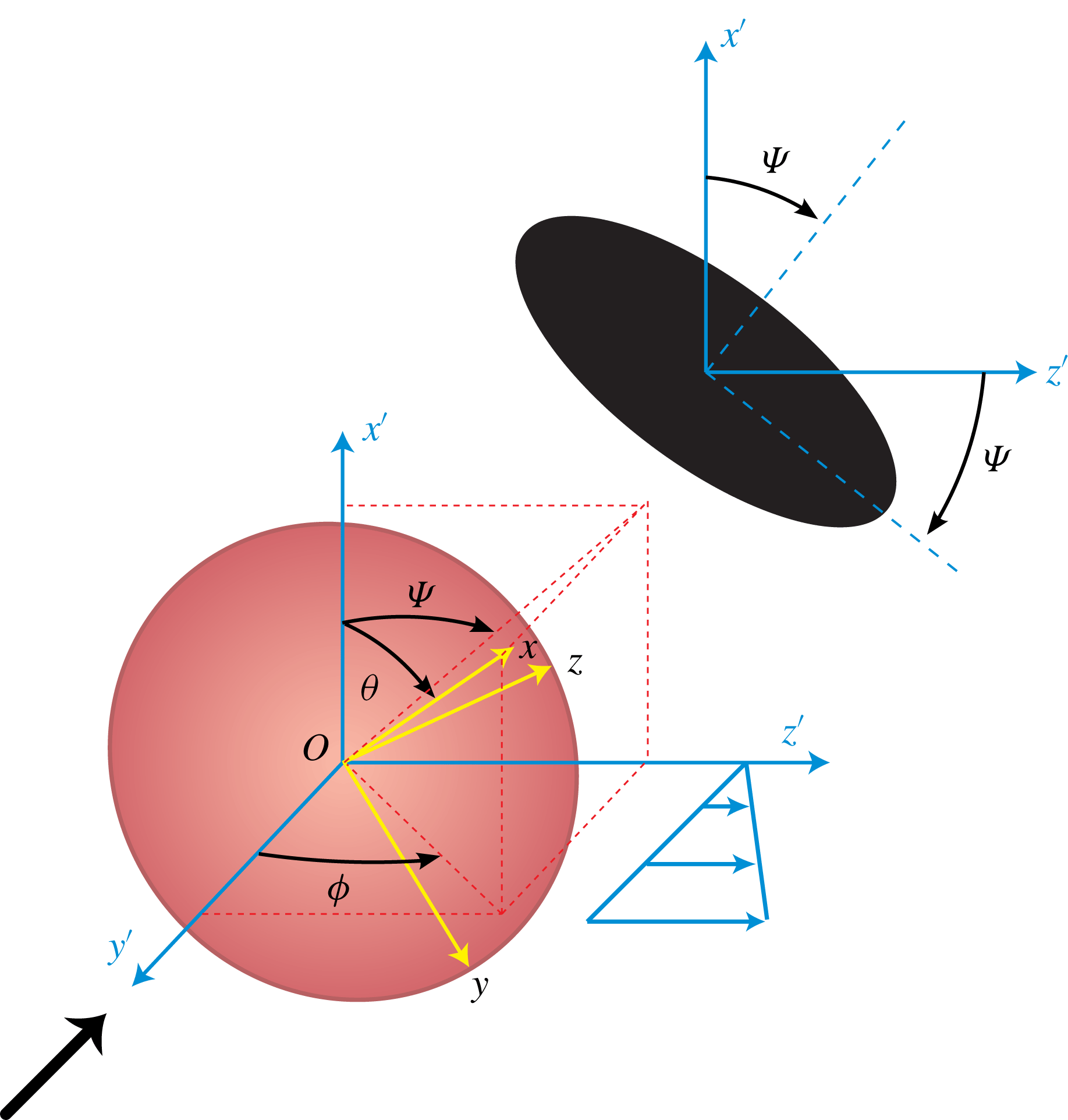
We consider cells placed in a shear flow with flow direction
 $Oz^{\prime }$
, shear gradient direction
 $Oy^{\prime }$
and vorticity axis
 $Ox^{\prime }$
. To characterize the orientation and motion of cells, we shall use the Euler angles. Let us consider, as a first approximation of RBC shape, an ellipsoid of the equation
 $$\begin{eqnarray}r^{2}x^{2}+y^{2}+z^{2}=1.\end{eqnarray}$$
Here
 $r$
is the aspect ratio, which will be larger than 1 here (oblate ellipsoid). This ellipsoid may rotate and we use the Euler angles as defined in Jeffery (Reference Jeffery1922) and in figure 1 to describe this rotation in the fixed coordinate system
 $Ox^{\prime }y^{\prime }z^{\prime }$
that coincides initially with the system
 $Oxyz$
associated with the ellipsoid (supplemental material is available online at https://doi.org/10.1017/jfm.2019.42 and presents a comparison with the other convention used in the literature).
In the original paper by Jeffery (Reference Jeffery1922),
 $\unicode[STIX]{x1D703}$
is obtained by rotation around the
 $Oz^{\prime }=Oz$
axis, then
 $\unicode[STIX]{x1D719}$
is obtained by rotation around the
 $Ox^{\prime }$
axis, such that it is defined as the angle between the planes
 $Ox^{\prime }y^{\prime }$
and
 $Ox^{\prime }x$
(see figure 1). With this convention, when
 $\unicode[STIX]{x1D719}=0$
and
 $\unicode[STIX]{x1D703}=90^{\circ }$
, the cell face is in the
 $Ox^{\prime }z^{\prime }$
plane.
If the cells are viewed from the velocity gradient axis
 $Oy^{\prime }$
, as in our experiments, the angle
 $\unicode[STIX]{x1D6F9}$
defined as the angle between
 $Ox^{\prime }$
and the projection of the cell axis of revolution
 $Ox$
onto the plane
 $Ox^{\prime }z^{\prime }$
, can be easily determined (see figure 1). This angle is also the angle between the projection of the cell and the flow direction. Here
 $\unicode[STIX]{x1D6F9}$
is related to
 $\unicode[STIX]{x1D703}$
and
 $\unicode[STIX]{x1D719}$
through
 $\tan \unicode[STIX]{x1D6F9}=\tan \unicode[STIX]{x1D703}\sin \unicode[STIX]{x1D719}$
.
The Euler angles used to describe the flipping regime. Convention used in Jeffery (Reference Jeffery1922) and in this paper. The large black arrow shows the viewing direction in the experiments, where projection onto the
 $x^{\prime }z^{\prime }$
plane is seen (black ellipse).

Selected snapshots along half a flipping period of an ellipsoid of aspect ratio
 $r=3$
following a Jeffery orbit of orbit angle
 $\unicode[STIX]{x1D703}_{0}=45^{\circ }$
. The black shape is the projection of the ellipsoid parallel in the shear gradient direction; it corresponds to what is seen in our experiment. Here
 $\unicode[STIX]{x1D6F9}$
is the angle of the main axis of this projected shape with the flow direction. As stated by (2.6), it oscillates between
 $-\unicode[STIX]{x1D703}_{0}$
and
 $\unicode[STIX]{x1D703}_{0}$
. The apparent aspect ratio
 $r_{a}$
oscillates between a minimal value strictly larger than 1 and
 $r$
, when the cell is seen edge on and
 $\unicode[STIX]{x1D6F9}=\pm \unicode[STIX]{x1D703}_{0}$
.

2.2 Jeffery orbits
For a shear flow in the
 $z^{\prime }$
direction with
 $y^{\prime }$
the shear gradient direction and
 $x^{\prime }$
the vorticity direction, the motion of a rigid ellipsoid in creeping flow is given by Jeffery (Reference Jeffery1922)
 $$\begin{eqnarray}\displaystyle & \displaystyle \dot{\unicode[STIX]{x1D703}}=\dot{\unicode[STIX]{x1D6FE}}\frac{r^{2}-1}{r^{2}+1}\sin \unicode[STIX]{x1D703}\cos \unicode[STIX]{x1D703}\sin \unicode[STIX]{x1D719}\cos \unicode[STIX]{x1D719}, & \displaystyle\end{eqnarray}$$
 $$\begin{eqnarray}\displaystyle & \displaystyle \dot{\unicode[STIX]{x1D719}}=\frac{\dot{\unicode[STIX]{x1D6FE}}}{1+r^{-2}}(r^{-2}\cos ^{2}\unicode[STIX]{x1D719}+\sin ^{2}\unicode[STIX]{x1D719}), & \displaystyle\end{eqnarray}$$
with
 $C\equiv r\tan \unicode[STIX]{x1D703}_{0}$
the orbit parameter. These equations can be solved and give
 $$\begin{eqnarray}\displaystyle & \displaystyle \tan \unicode[STIX]{x1D703}=\frac{C}{r(r^{-2}\cos ^{2}\unicode[STIX]{x1D719}+\sin ^{2}\unicode[STIX]{x1D719})^{1/2}}, & \displaystyle\end{eqnarray}$$
 $$\begin{eqnarray}\displaystyle & \displaystyle \tan \unicode[STIX]{x1D719}=r^{-1}\tan \frac{\dot{\unicode[STIX]{x1D6FE}}t}{r+r^{-1}}. & \displaystyle\end{eqnarray}$$
Here
 $\unicode[STIX]{x1D703}$
oscillates between
 $\unicode[STIX]{x1D703}_{0}$
and
 $\arctan C$
(spinning motion).
We shall refer to these possible motions as flipping motions. Among them,
 $\unicode[STIX]{x1D703}_{0}=0^{\circ }$
corresponds to what is called rolling motion (
 $\unicode[STIX]{x1D703}$
always equal to 0), while
 $\unicode[STIX]{x1D703}_{0}=90^{\circ }$
corresponds to tumbling (
 $\unicode[STIX]{x1D703}$
always equal to
 $90^{\circ }$
). Note that when
 $r>1$
,
 $\dot{\unicode[STIX]{x1D719}}$
is minimal when
 $\unicode[STIX]{x1D719}=0$
, which corresponds to the cell aligned with the flow direction.
Simple trigonometry then yields the equation for
 $\unicode[STIX]{x1D6F9}(t)$
according to Jeffery theory:
 $$\begin{eqnarray}\tan \unicode[STIX]{x1D6F9}=\tan \unicode[STIX]{x1D703}_{0}\times \sin \frac{\dot{\unicode[STIX]{x1D6FE}}t}{r+r^{-1}}.\end{eqnarray}$$
Therefore,
 $\unicode[STIX]{x1D6F9}$
oscillates between two extreme positions
 $-\unicode[STIX]{x1D703}_{0}$
and
 $\unicode[STIX]{x1D703}_{0}$
, where it stays for more time (see figure 2 for an example).
In this paper, we shall consider the possible flipping motions for a cell, that will be hypothesized to closely follow Jeffery orbits, but also the tank-treading motion. In that case, the cell small axis remains in the shear plane (
 $\unicode[STIX]{x1D703}=90^{\circ }$
) while the cell adopts a constant angle relatively to the flow direction. This definition is unambiguous as long as the cell does not deform. If it does, as pointed out in Dupont et al. (Reference Dupont, Delahaye, Barthès-Biesel and Salsac2016) where oblate capsules are considered, one should refer to the membrane material point that was located, at rest, on the small axis. From this unambiguous definition, a cell of fixed shape in flow for which this point is directed toward the vorticity direction would be called a rolling cell, even though its deformation is such that it resembles a tank-treading cell. From this point of view, the tank-treading motion mentioned in Cordasco, Yazdani & Bagchi (Reference Cordasco, Yazdani and Bagchi2014, figure 12) or in Sinha & Graham (Reference Sinha and Graham2015, figure 15) should be called rolling motion.
Since the numerical studies we will refer to in the following have used the term tank-treading, and since in most experimental studies the deformation seems to remain weak, we shall however go on using the (potentially improper) term of tank-treading for cells whose small axis of symmetry lies in the shear plane.
3 State of the art
Throughout this paper and in this section in particular, we shall use the Jeffery notation and conventions (figure 1). The original notation used in the considered papers (which are quite varied) are recalled in the supplemental material, for the sake of clarity. Experiments were run at laboratory temperature, at which the viscosity of the haemoglobin solution is close to 10 mPa s, when it is equal to 6.5 mPa s at body temperature. In experimental papers, the ‘natural’ parameter space
 $(\unicode[STIX]{x1D702}_{0},\dot{\unicode[STIX]{x1D6FE}})$
is often used, where
 $\unicode[STIX]{x1D702}_{0}$
is the carrying fluid viscosity and
 $\dot{\unicode[STIX]{x1D6FE}}$
the shear rate, a parameter that can be varied continuously. As an alternative to
 $\dot{\unicode[STIX]{x1D6FE}}$
, the typical stress on the cell
 $\unicode[STIX]{x1D70F}=\unicode[STIX]{x1D702}_{0}\dot{\unicode[STIX]{x1D6FE}}$
is also often considered. We shall stick to this latter choice in the following.
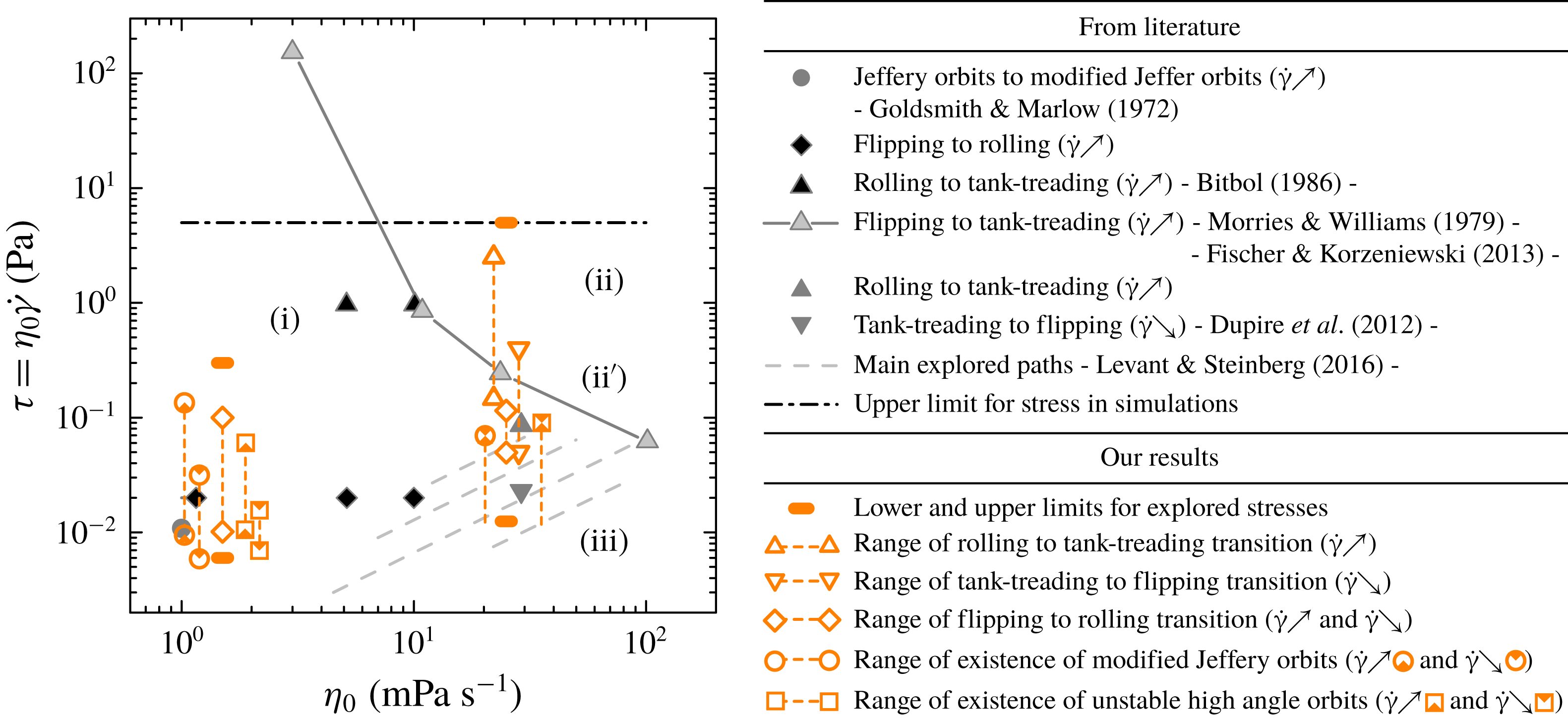
The main thresholds and dynamics states domains found in previous experiments from the literature are reported in figure 3.
In numerical simulations, dimensionless parameters are naturally chosen. These are
 $\unicode[STIX]{x1D706}$
and
 $C_{a}$
. Here
 $\unicode[STIX]{x1D706}$
is the viscosity contrast, that is, the ratio between the viscosity of the haemoglobin solution and that of the carrying fluid. Therefore,
 $\unicode[STIX]{x1D706}=1$
corresponds to
 $\unicode[STIX]{x1D702}_{0}\simeq 10~\text{mPa}~\text{s}$
in the experiments. The capillary number
 $C_{a}$
compares the flow stress
 $\unicode[STIX]{x1D702}_{0}\dot{\unicode[STIX]{x1D6FE}}$
with the elastic stress:
 $C_{a}=\unicode[STIX]{x1D702}_{0}\dot{\unicode[STIX]{x1D6FE}}R/\unicode[STIX]{x1D707}$
, where
 $R$
is the typical size of the RBC and
 $\unicode[STIX]{x1D707}$
the shear elasticity modulus of the membrane. Here
 $\unicode[STIX]{x1D702}_{0}$
is typically varied between 1 and 100 mPa s and the stress
 $\unicode[STIX]{x1D702}_{0}\dot{\unicode[STIX]{x1D6FE}}$
does not exceed 5 Pa (20 Pa in the more recent Mauer et al. (Reference Mauer, Mendez, Lanotte, Nicoud, Abkarian, Gompper and Fedosov2018)). Technical details and a description of the main results of the most recent and relevant papers that we consider here are reported in the supplemental material and will be recalled when necessary in the discussion of our results.
All recent simulation papers establish a diagram that is qualitatively coherent with that partly drawn by experiments (see Cordasco & Bagchi Reference Cordasco and Bagchi2013; Cordasco et al.
Reference Cordasco, Yazdani and Bagchi2014; Peng et al.
Reference Peng, Mashayekh and Zhu2014; Sinha & Graham Reference Sinha and Graham2015; Mendez & Abkarian Reference Mendez and Abkarian2018). This diagram can be divided into four zones, the frontier of which depends on the considered equilibrium shapes (see figure 3): (i) flipping motions, (ii) tank-treading, (ii
 $^{\prime }$
) tank-treading like motions with oscillations or slightly off-plane motion, (iii) flipping motions, but orbit stability is different than in the low external viscosity case (i). The intermediate region (ii
 $^{\prime }$
) corresponds to a narrow range in the parameter space. In all papers, the different regimes are obtained by starting with a cell with a given orientation
 $\unicode[STIX]{x1D703}$
, and following its time evolution. From the way the simulations are run, we can consider that they correspond more to the increasing
 $\dot{\unicode[STIX]{x1D6FE}}$
case (but to a sharp increase). None of the previous studies consider the decreasing case or the smoothly increasing case.
Summary of the transition thresholds identified in the literature and in our experiments. Whether the mentioned transition should be understood to occur in the increasing or decreasing shear rate case is indicated by the symbols (
 $\dot{\unicode[STIX]{x1D6FE}}{\nearrow}$
) and (
 $\dot{\unicode[STIX]{x1D6FE}}{\searrow}$
), respectively. The chosen data points from the literature are commented on in the text. Owing to variability between cells, all of our thresholds are identified by an interval. Some transitions have no lower bound because of the range of stresses explored. The transition intervals are slightly shifted around the two explored viscosities
 $1.5$
and 25 mPa s for clarity.

3.1 Experimental papers
One of the first major contributions to the study of RBC dynamics under shear flow can be found in Goldsmith & Marlow (Reference Goldsmith and Marlow1972) where statistics on the angle distribution is obtained. They observed dilute RBCs in a large tube where, at the cell scale, the flow can be assimilated to simple shear flow, with the same outer viscosity
 $\unicode[STIX]{x1D702}_{0}$
as plasma. They also performed experiments in a plate geometry at high
 $\unicode[STIX]{x1D702}_{0}$
(520 mPa s) and low
 $\dot{\unicode[STIX]{x1D6FE}}$
(around
 $1~\text{s}^{-1}$
). Both experiments correspond to an increasing
 $\dot{\unicode[STIX]{x1D6FE}}$
: in the Poiseuille flow experiment the observation tube is narrower than the upstream tubes, and in the shear chamber experiment, RBCs are initially at rest.
The main outcomes of Goldsmith and Marlow’s study are as follows.
(i) In plasma and at low shear rate (
 $\dot{\unicode[STIX]{x1D6FE}}<10~\text{s}^{-1},\unicode[STIX]{x1D70F}<0.01~\text{Pa}$
), the time evolution
$\unicode[STIX]{x1D719}(t)$
can be well described by Jeffery’s equation (2.5) if an effective aspect ratio is introduced, which is 25 % lower than the aspect ratio of the convex envelope of the cell. This result was previously found for rigid circular disks (Anczurowski & Mason Reference Anczurowski and Mason1967), and the discrepancy between the two ratios is expected to decrease as the aspect ratio gets closer to 1.
(ii) At higher
$\dot{\unicode[STIX]{x1D6FE}}$
, departure from Jeffery’s equation is observed, with longer duration of alignment with flow and the initial
$\unicode[STIX]{x1D719}\rightarrow -\unicode[STIX]{x1D719}$
symmetry for
$\dot{\unicode[STIX]{x1D719}}$
is lost. This is interpreted as the consequence of cell deformability, which induces different shapes depending on the cell orientation relatively to the extensional direction of the flow. At the same time, more cells drift into rolling motion (
$\unicode[STIX]{x1D703}=0$
). Those feature are lost for hardened cells.(iii) Contrary to what the Jeffery theory states,
$\unicode[STIX]{x1D703}$
was found not to be periodic as a function of
$\unicode[STIX]{x1D719}$
, and the motion appears to be less regular. This is interpreted as a consequence of rotary Brownian motion of cells.(iv) In the highly viscous suspending medium, cells are seen to align strongly with the flow. However, no clear discrimination is made between tank-treading and rolling cells.


The drift to rolling is studied in Bitbol (Reference Bitbol1986). The cells were observed in a cone-plate geometry allowing for
 $\dot{\unicode[STIX]{x1D6FE}}$
between 1 and
 $200~\text{s}^{-1}$
. Viscosity
 $\unicode[STIX]{x1D702}_{0}$
of the suspending medium was between 1 and 10 mPa s. The main results are as follows.
(i) If one considers the single parameter
$\unicode[STIX]{x1D70F}=\unicode[STIX]{x1D702}_{0}\dot{\unicode[STIX]{x1D6FE}}$
, which measures the flow stress on the cell, a rough phase diagram is obtained from direct observations as follows: if
$\unicode[STIX]{x1D70F}<0.02~\text{Pa}$
, cells rotate in the flow (that is, flipping motion is observed). In the intermediate range
$0.02~\text{Pa}<\unicode[STIX]{x1D70F}<1~\text{Pa}$
, cells drift to rolling. For higher stresses, the number of rolling cells plateaus at viscosity
$\unicode[STIX]{x1D702}_{0}=1~\text{mPa}~\text{s}$
while it decreases when
$\unicode[STIX]{x1D702}_{0}>5~\text{mPa}~\text{s}$
: cells start to tank-tread.(ii) In the rolling regime, the cell diameter increases with
$\unicode[STIX]{x1D702}_{0}$
and
$\dot{\unicode[STIX]{x1D6FE}}$
, as already found in Goldsmith & Marlow (Reference Goldsmith and Marlow1972).(iii) In the considered viscosity range, the typical time for cell drift towards rolling is of the order of
$100\times \dot{\unicode[STIX]{x1D6FE}}^{-1}$
.


Several new features were highlighted in Dupire et al. (Reference Dupire, Socol and Viallat2012), which followed a first paper by the same group (see Abkarian et al.
Reference Abkarian, Faivre and Viallat2007). In these papers, the case of decreasing
 $\dot{\unicode[STIX]{x1D6FE}}$
is considered for the first time, and off-shear plane motion is also described for the first time. The carrying fluid viscosities
 $\unicode[STIX]{x1D702}_{0}$
are 7 and 29 mPa s, and the
 $\dot{\unicode[STIX]{x1D6FE}}$
goes from 0 to
 $15~\text{s}^{-1}$
in the first case and to
 $2.7~\text{s}^{-1}$
in the second case. The cells flow in a large parallelepiped flow chamber where around 20 cells were tracked individually and visualized along both the shear and vorticity axes. The main results of this paper are as follows.
(i) At low
$\dot{\unicode[STIX]{x1D6FE}}$
, the orbit angle
$\unicode[STIX]{x1D703}_{0}$
of a flipping cell is not constant but varies between
$50^{\circ }$
and
$90^{\circ }$
.(ii) If the shear rate exceeds a threshold
$\dot{\unicode[STIX]{x1D6FE}}_{t}$
lying between 0.01 and 0.05 Pa depending on the observed cell, this orbit angle stabilizes to a constant value (that decreases with
$\dot{\unicode[STIX]{x1D6FE}}$
, until the rolling regime is reached).(iii) In the flipping regime, the time evolution of
$\unicode[STIX]{x1D719}$
is well described by the Jeffery equation.(iv) At some critical shear rate
$\dot{\unicode[STIX]{x1D6FE}}_{c}^{+}$
, transition towards tank-treading is observed. Tank-treading is associated to swinging, that is, periodic oscillation of the inclination angle.(v) If
$\dot{\unicode[STIX]{x1D6FE}}$
is then decreased, the tank-treading motion remains stable until some other critical shear rate
$\dot{\unicode[STIX]{x1D6FE}}_{c}^{-}<\dot{\unicode[STIX]{x1D6FE}}_{c}^{+}$
at which a transient intermittent regime is observed. It shows an alternance (in time) between tank-treading and flipping motions with high
$\unicode[STIX]{x1D703}_{0}$
. When an orbit angle lower than
$50^{\circ }$
is reached, flipping motion with a fixed orbit angle becomes stable, with the same orbit angle equal to that observed for the same shear rate in the increasing
$\dot{\unicode[STIX]{x1D6FE}}$
case. From this observation we deduce that
$\dot{\unicode[STIX]{x1D6FE}}_{t}<\dot{\unicode[STIX]{x1D6FE}}_{c}^{-}$
. Although not explicitly stated in Dupire et al. (Reference Dupire, Socol and Viallat2012), it seems that upon a further decrease of
$\dot{\unicode[STIX]{x1D6FE}}$
the same branch as in the increasing
$\dot{\unicode[STIX]{x1D6FE}}$
case is followed.(vi) There is no variation in
$\dot{\unicode[STIX]{x1D6FE}}_{c}^{-}$
and
$\dot{\unicode[STIX]{x1D6FE}}_{c}^{+}$
if many shear rate cycles are applied to the same cell. The corresponding critical shear stress values are 0.023 and 0.086 Pa for
$\unicode[STIX]{x1D702}_{0}=29~\text{mPa}~\text{s}$
. These are mean values, because all the critical stresses, as well as the orbit angles associated with a given stress, depend on the considered cell.(vii) All these transitions occur in a shape preserving manner, with diameter variations that remains lower than 10 %.


The transition between flipping and tank-treading for several viscosities and many cells is studied in Fischer & Korzeniewski (Reference Fischer and Korzeniewski2013). They consider a Poiseuille flow, so it is likely that only the increasing
 $\dot{\unicode[STIX]{x1D6FE}}$
case is considered, though we do not know what the upstream conditions are. The critical
 $\dot{\unicode[STIX]{x1D6FE}}$
for
 $\unicode[STIX]{x1D702}_{0}=11,24$
and 104 mPa s are 75, 10 and
 $0.6~\text{s}^{-1}$
, respectively. The transition shear rate is determined as the value at which half of the RBCs are in tank-treading regime. The authors also establish that the transition is not sharp: the number of cells in tank-treading increases smoothly with the
 $\dot{\unicode[STIX]{x1D6FE}}$
. The transition becomes more abrupt at high carrying fluid viscosity
 $\unicode[STIX]{x1D702}_{0}$
. Those thresholds together with that measured in Morris & Williams (Reference Morris and Williams1979) for plasma viscosity, allow a separation line to be drawn between flipping-like motion and tank-treading-like motion in the (
 $\unicode[STIX]{x1D702}_{0},\unicode[STIX]{x1D70F}$
) space, as shown in figure 3.
In Lanotte et al. (Reference Lanotte, Mauer, Mendez, Fedosov, Fromental, Claveria, Nicoud, Gompper and Abkarian2016), experiments similar to those in Fischer & Korzeniewski (Reference Fischer and Korzeniewski2013) are performed in physiological condition, but on a limited amount of cells. Transitions from flipping to rolling are observed from
 $\dot{\unicode[STIX]{x1D6FE}}=10~\text{s}^{-1}$
until
 $\dot{\unicode[STIX]{x1D6FE}}=40~\text{s}^{-1}$
(
 $\unicode[STIX]{x1D70F}=0.04~\text{Pa}~\text{s}$
). In the meantime and also for larger shear rates, an increasing proportion of cup-shaped stomatocytes in rolling motion is detected. At even higher shear rates (until the maximum considered,
 $\dot{\unicode[STIX]{x1D6FE}}=2000~\text{s}^{-1}$
), highly deformed polylobed shapes are observed. No notion of increasing or decreasing
 $\dot{\unicode[STIX]{x1D6FE}}$
is introduced in these experiments. They confirmed this picture in a second recent paper with shear rates higher than
 $60~\text{s}^{-1}$
(see Mauer et al.
Reference Mauer, Mendez, Lanotte, Nicoud, Abkarian, Gompper and Fedosov2018).
Finally, in Levant & Steinberg (Reference Levant and Steinberg2016), 17 cells are studied in a four roll mill apparatus which allows to consider a more general flow defined by the vorticity
 $\unicode[STIX]{x1D714}$
and the strain rate
 $s$
. Simple shear flow corresponds to the case
 $2\unicode[STIX]{x1D714}=2s=\dot{\unicode[STIX]{x1D6FE}}$
. It corresponds to a stability threshold for the apparatus, since
 $\unicode[STIX]{x1D714}/s>1$
is required for the cell to remain trapped. Long time observation is then possible, while varying the ratio
 $\unicode[STIX]{x1D714}/s$
. More precisely,
 $\unicode[STIX]{x1D714}$
is fixed and
 $s$
is varied. The explored range of external viscosities is 20–87 mPa s. The possibility to increase the contribution of the vorticity allows to switch to flipping regimes even in that viscosity range. With the choice to characterize the flow stress by
 $2s\unicode[STIX]{x1D702}_{0}$
and to consider the extended viscosity
 $\unicode[STIX]{x1D702}_{0}(w/s)^{-1}$
, three regions are identified, corresponding to tumbling, swinging, and an intermittent regime, which coincide with those identified in Dupire et al. (Reference Dupire, Socol and Viallat2012). Contrary to what was observed in Dupire et al. (Reference Dupire, Socol and Viallat2012), large deformations are associated with the intermittent regime. Although the stress seems to be increased and decreased within the same experiment, no hysteretic behaviour is reported. In figure 3, the explored area in the
 $(\unicode[STIX]{x1D702}_{0}(w/s)^{-1},2s\unicode[STIX]{x1D702}_{0})$
parameter space is shown on the phase diagram for simple shear rate with parameter space
 $(\unicode[STIX]{x1D702}_{0},\unicode[STIX]{x1D702}_{0}\dot{\unicode[STIX]{x1D6FE}})$
. We shall note that, in agreement with numerical simulations in Cordasco & Bagchi (Reference Cordasco and Bagchi2013), no off-plane motion is observed in the flipping region, while it is seen in simple shear flow in Dupire et al. (Reference Dupire, Socol and Viallat2012). This partial mapping shows that an increased rotational component in the flow, as in Levant & Steinberg (Reference Levant and Steinberg2016), favours in-plane motion.
The experimental studies summarized above have all brought new features to the problem. They neither contradict each other nor provide cross-validation since the explored parameter ranges, or the experimental method, often differ. Studies on individual cells that are followed in time have allowed more detailed dynamics to be exhibited (see Abkarian et al.
Reference Abkarian, Faivre and Viallat2007; Dupire et al.
Reference Dupire, Socol and Viallat2012; Levant & Steinberg Reference Levant and Steinberg2016), but full characterization of the transition dynamics could not be addressed, in particular concerning the consequence of dispersion in size and mechanical properties of cells. The decreasing
 $\dot{\unicode[STIX]{x1D6FE}}$
case has only been clearly addressed in Dupire et al. (Reference Dupire, Socol and Viallat2012). On the other hand studies on statistically relevant populations are often limited to the study of a single feature, e.g. the population in tank-treading regime (see Goldsmith & Marlow Reference Goldsmith and Marlow1972; Fischer & Korzeniewski Reference Fischer and Korzeniewski2013) or in deformed rolling regime (see Mauer et al.
Reference Mauer, Mendez, Lanotte, Nicoud, Abkarian, Gompper and Fedosov2018), but they allowed the width of transition zones due to cell dispersity to be estimated, in the increasing
 $\dot{\unicode[STIX]{x1D6FE}}$
case only.
The case of physiological values for the external fluid viscosity has seldom been addressed, probably because of sedimentation issues, and is therefore much less documented than the case of more viscous fluids.
3.2 On the hysteresis and the intermittent regimes
A striking feature is the existence, at least for high enough viscosities of the external fluid, of an hysteresis in the
 $(\unicode[STIX]{x1D702}_{0},\dot{\unicode[STIX]{x1D6FE}})$
space upon variations of
 $\dot{\unicode[STIX]{x1D6FE}}$
, which has been described differently in different papers. We aim at clarifying this in the following.
In the first experimental paper to account for such a feature (see Abkarian et al.
Reference Abkarian, Faivre and Viallat2007), the observed low shear rate motion is surprisingly always tumbling. Transition to tank-treading (or, rather, swinging) is characterized by the existence of an intermediate regime where cells alternatively tumble and swing, which is observed for both decreasing and increasing
 $\dot{\unicode[STIX]{x1D6FE}}$
. The experimental constraints did not allow a conclusion on whether this intermittent regime is transient or not. Transition shear rates denoted
 $\dot{\unicode[STIX]{x1D6FE}}_{c}^{{>}}$
and
 $\dot{\unicode[STIX]{x1D6FE}}_{c}^{{<}}$
are identified, with
 $\dot{\unicode[STIX]{x1D6FE}}_{c}^{{>}}>\dot{\unicode[STIX]{x1D6FE}}_{c}^{{<}}$
, a signature of hysteretic behaviour. They correspond respectively to the first observed transition from tumbling to swinging when increasing
 $\dot{\unicode[STIX]{x1D6FE}}$
and to the first observed transition from swinging to tumbling when decreasing
 $\dot{\unicode[STIX]{x1D6FE}}$
, for an observation over a time scale of order 20s.
In the same paper, an improvement of the analytical model by Keller & Skalak (Reference Keller and Skalak1982) (a droplet enclosed by an ellipsoidal fluid membrane) is proposed for RBC dynamics. Membrane shear elasticity is taken into account (as, simultaneously, in Skotheim & Secomb (Reference Skotheim and Secomb2007)), and in Dupire et al. (Reference Dupire, Abkarian and Viallat2015) the possibility for a stress-free configuration different from the equilibrium shape is explored. In that model, considering more inflated stress-free configurations amounts to multiplying the shear modulus by some constant smaller than 1. Considering the transition threshold and other characteristics such as cell oscillation periods, it was deduced in Dupire et al. (Reference Dupire, Abkarian and Viallat2015) that the stress-free configuration is likely to be a spheroid, in agreement with other modelling approaches (see Lim, Wortis & Mukhopadhyay Reference Lim, Wortis and Mukhopadhyay2002; Cordasco & Bagchi Reference Cordasco and Bagchi2014; Peng et al.
Reference Peng, Mashayekh and Zhu2014). Returning to our initial question, the analytical model results in differential equations for the angles characterizing cell dynamics, for the case where the cell axis of symmetry remains in the shear plane. In other words, only transitions between tumbling-like and tank-treading-like motions can be explored (a recent model proposed by Mendez & Abkarian (Reference Mendez and Abkarian2018) should solve this issue in the future). These equations can be solved numerically for a given shear rate and a given set of parameters for the cell mechanical properties, and an intermittent regime is observed in an interval
 $[\dot{\unicode[STIX]{x1D6FE}}_{c}^{-};\dot{\unicode[STIX]{x1D6FE}}_{c}^{+}]$
. In Abkarian et al. (Reference Abkarian, Faivre and Viallat2007) or in Dupire et al. (Reference Dupire, Abkarian and Viallat2015) it is however not specified whether the threshold values are obtained by considering increasing or decreasing
 $\dot{\unicode[STIX]{x1D6FE}}$
. Knowing the dependency of the solutions of the cell angle evolution equations on the history of
 $\dot{\unicode[STIX]{x1D6FE}}$
values probably requires a precise stability analysis such as that done in Kessler et al. (Reference Kessler, Finken and Seifert2009) in the case of quasi-spherical cells.
Though they are clearly related to each other, how the different thresholds
 $\dot{\unicode[STIX]{x1D6FE}}_{c}^{\langle ,\rangle }$
and
 $\dot{\unicode[STIX]{x1D6FE}}_{c}^{-,+}$
compare with each other is not clear as they were determined differently (limited observation time in the experiments and more importantly no direct study of potential hysteresis in the numerical analysis).
The intermittent behaviour has been observed and thoroughly studied using numerical simulations (starting from a rest configuration) in Cordasco & Bagchi (Reference Cordasco and Bagchi2014) and in Peng et al. (Reference Peng, Mashayekh and Zhu2014), with the axis of revolution also restricted to shear plane, though in some cases this configuration is said to be metastable according to Cordasco & Bagchi (Reference Cordasco and Bagchi2014). In Peng et al. (Reference Peng, Mashayekh and Zhu2014), the minor bound
 $\dot{\unicode[STIX]{x1D6FE}}_{c}^{-}$
of the intermittent regime is determined and shown to be smaller than the transition shear rate between rolling and tank-treading. Finally, in the experimental paper by Levant & Steinberg (Reference Levant and Steinberg2016) a stationary intermittent regime is also observed for, apparently, increasing and decreasing flow stress although it is only explicitly highlighted for a decrease of the flow stress
 $2s\unicode[STIX]{x1D702}_{0}$
. Note that in this paper the flow geometry is not the same and no off-shear plane motion is observed.
In Dupire et al. (Reference Dupire, Socol and Viallat2012), the picture turns out to be more complex: the decreasing
 $\dot{\unicode[STIX]{x1D6FE}}$
path would be characterized by the apparition of a transient intermittent (tank-treading/flipping with angle larger than
 $50^{\circ }$
) phase when tank-treading regime is left, whose duration in time is not clear. After this intermittent phase, flipping motion with orbit angle strictly smaller than
 $50^{\circ }$
would follow. The shear rate at which this transition takes place is denoted by
 $\dot{\unicode[STIX]{x1D6FE}}_{c}^{-}$
, and no notion of interval over which this intermittent regime would be possible is introduced. The analogy with the notation
 $\dot{\unicode[STIX]{x1D6FE}}_{c}^{-}$
introduced in Abkarian et al. (Reference Abkarian, Faivre and Viallat2007) suggests that the transient intermittent regime would only take place in the low part of the whole expected range for the intermittent regime
 $[\dot{\unicode[STIX]{x1D6FE}}_{c}^{-};\dot{\unicode[STIX]{x1D6FE}}_{c}^{+}]$
, while stable tank-treading would be preferred in the top range.
On the other hand, upon an increase of shear rate, no intermittent regime is observed but rather a continuous drift from tumbling to rolling, then a transition to swinging. In Dupire et al. (Reference Dupire, Socol and Viallat2012), the threshold for this transition is denoted by
 $\dot{\unicode[STIX]{x1D6FE}}_{c}^{+}$
, suggesting that when increasing
 $\dot{\unicode[STIX]{x1D6FE}}$
the route to swinging through the intermittent regime is replaced by the orbital drift. In Levant & Steinberg (Reference Levant and Steinberg2016), the intermittent regime is associated with large cell deformations: we hypothesize that the orbital drift is another route that prevents such large elastic distortions. This would explain why the intermittent regime is not seen in the increasing shear rate case, unless forced by restricting the motion to the shear plane, artificially in the simulations or because of a specific flow geometry as in Levant & Steinberg (Reference Levant and Steinberg2016).
Finally, the fact that, to the best of the authors’ knowledge, no analytical or numerical analysis has considered the decreasing shear rate case so far limits the discussion on the relationship between hysteretic and (possibly transient) intermittent regimes. A secondary goal of the present study is to reinforce the experimental input on this question.
4 Experiments
Blood samples from healthy donors were tested and provided by the French blood bank EFS. To remove all substances except RBCs, the samples were centrifuged and washed in physiological buffer solution (phosphate buffered saline (PBS), Sigma). This procedure was repeated three times at room temperature; after each centrifugation, the liquid phase and buffy coat were removed by aspiration. Then RBCs were resuspended either in PBS solution with
 $1~\text{g}~\text{L}^{-1}$
of bovine serum albumin (BSA, Sigma) or in a PBS
 $+$
BSA solution where dextran was diluted (
 $20~\text{g}~\text{L}^{-1}$
of dextran of molecular weight
 $1.5\times 10^{4}+70~\text{g}~\text{L}^{-1}$
of dextran of molecular weight
 $2\times 10^{6}$
). This latter solution has a viscosity at room temperature (
 $23{-}25\,^{\circ }\text{C}$
) of
 $25\pm 0.5$
mPa s, a configuration close to that often considered in the literature. The viscosity and density of this solution are such that they allow long-time acquisition without sedimentation issues.
By contrast, cells in plasma quickly sediment, with a velocity of typically
 $1~\unicode[STIX]{x03BC}\text{m}~\text{s}^{-1}$
. This prevents long-time observations in flow chambers adapted to microscopy. In order to counterbalance sedimentation, water in the PBS solution was replaced by a mixture of 68.5 % water and 31.5 % Optiprep© (iodixanol solution, Axis-Shield), so as to reach a density close to that of cells (
 $1.1~\text{g}~\text{ml}^{-1}$
), following a method initially proposed in Roman et al. (Reference Roman, Lorthois, Duru and Risso2012) and subsequently used in Shen et al. (Reference Shen, Coupier, Kaoui, Polack, Harting, Misbah and Podgorski2016) and Roman et al. (Reference Roman, Merlo, Duru, Risso and Lorthois2016). This solution has a viscosity at room temperature of
 $1.5\pm 0.1$
mPa s, close to that of plasma (1.95 mPa s at
 $20\,^{\circ }\text{C}$
, and 1.34 mPa s at
 $37\,^{\circ }\text{C}$
(see Brust et al.
Reference Brust, Schaefer, Doerr, Pan, Garcia, Arratia and Wagner2013)).
In all suspensions, the volume fraction is very weak (
 ${\sim}0.01\,\%$
), and cells are located everywhere in the chamber: one can consider the cells are isolated and do not interact hydrodynamically. The suspension is injected into a plane–plane shear chamber of gap
 $200~\unicode[STIX]{x03BC}\text{m}$
as described previously in Callens et al. (Reference Callens, Minetti, Coupier, Mader, Dubois, Misbah and Podgorski2008). The shear rate
 $\dot{\unicode[STIX]{x1D6FE}}$
is varied step by step from
 $0.5~\text{s}^{-1}$
to
 $200~\text{s}^{-1}$
, then decreased back. The flow stress ranges are, thus,
 $7.5\times 10^{-4}~\text{Pa}$
to 0.3 Pa and
 $1.3\times 10^{-2}~\text{Pa}$
to 5 Pa for the low- and high-viscosity solutions, respectively. Those ranges are indicated in figure 3 for a comparison with the ranges explored in the literature. Owing to the low sedimentation rate, one sequence of increasing or decreasing shear rate could last around 1 h, with the same RBCs in the chamber all along the experiment. Thus, small steps for shear rate variation could be imposed, so as to obtain a precise diagram of the RBC dynamics. At each value of
 $\dot{\unicode[STIX]{x1D6FE}}$
, between 1 and 5 (for low shear rates) series of 600 images are taken at 24 fps. Series are separated by at least 15 s. Using several series allow good enough statistics to be obtained on the shape and orientation of the cells. Only cells located at
 $20~\unicode[STIX]{x03BC}\text{m}$
or further from the walls are included in the analysis, because the presence of walls may have an impact on the cell dynamics, in particular flipping motion (see Vitkova et al.
Reference Vitkova, Coupier, Mader, Kaoui, Misbah and Podgorski2009).
The RBC suspension is monitored by digital holographic microscopy (DHM) working in reduced spatial coherence, whose optical axis is perpendicular to the chamber planes. This configuration allows a strong reduction of the inherent noise of interferometry and provides better in-depth reconstruction capabilities (see Grandchamp et al. Reference Grandchamp, Coupier, Srivastav, Minetti and Podgorski2013; Minetti et al. Reference Minetti, Vitkova, Dubois and Bivas2016). On the basis of the acquired interferogram, it is possible to extract the complex amplitude of the optical beam passing through the sample and simulate numerically the propagation of the beam through the whole thickness of the experimental cell. In this way one can scan, slide by slide, the experimental volume and refocus numerically all the RBCs present in the suspension volume. The procedure to extract the three-dimensional position and features of each cell in the experimental volume is similar to that used in Minetti et al. (Reference Minetti, Podgorski, Coupier and Dubois2014) for lipid vesicles. RBCs require more attention in the data treatment than vesicles because their convex shape leads to a much higher distortion of the light beam, a property that was recently used to characterize cell morphologies (see Miccio et al. Reference Miccio, Memmolo, Merola, Netti and Ferraro2015). The projection of the cell shape on the plane perpendicular to the shear gradient direction is obtained, where each pixel intensity is proportional to the optical thickness (thickness of the cell times the difference of refractive index between the cell and the suspending fluid) in the optical axis direction. A segmentation is applied on each cell to determine the geometrical boundaries of the projected shape.
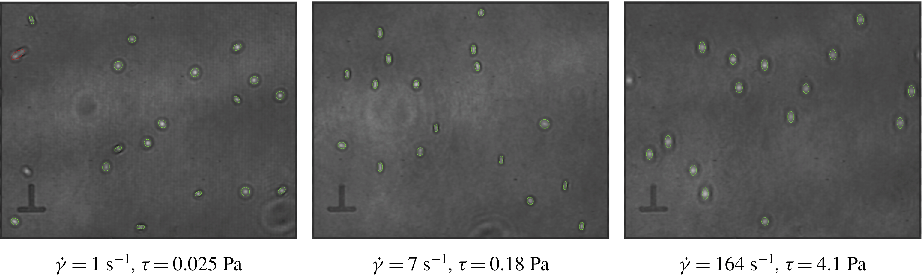
Example DHM images after treatment. The green contours are the fits of the cells projected shapes and the red contours correspond to those that were discarded because the aspect ratio or the apparent surface are considered as non-realistic. They mostly correspond to superimposed cells. Owing to the low concentration in cells, those patterns are scarce and, whatever the exclusion criterion considered, do not have much influence on the analysis.

For each detected cell, its major axis is determined from the diagonalization of the inertia matrix of its projected shape. This axis makes an angle
 $\unicode[STIX]{x1D6F9}$
with respect to the flow direction, as defined is § 2.1. Here
 $\unicode[STIX]{x1D6F9}$
is defined in the range
 $[0,90^{\circ }]$
. Taking this axis as an origin for angle
 $\unicode[STIX]{x1D709}$
, the contour of the projection of the cell is fitted by the polar equation
 $\unicode[STIX]{x1D70C}(\unicode[STIX]{x1D709})=\unicode[STIX]{x1D70C}_{0}+a_{1}\cos ^{2}\unicode[STIX]{x1D709}+a_{2}\cos ^{4}\unicode[STIX]{x1D709}+a_{3}\cos ^{6}\unicode[STIX]{x1D709}$
, which allows shapes that are more rod-like than ellipse-like to also be described, as is the case when viewed from the side. In that case, they may also appear as concave, because of the smaller contribution of the outer ring to the total optical thickness of the object. Examples of obtained images with the associated contours are shown in figure 4. The weight of the contribution of the outer ring can vary a lot depending on the orientation or position of the cell; for that reason we consider the aspect ratio
 $r_{a}$
of the convex envelope of the cell (that is, its effective projection) rather than the ratio between the radii at
 $\unicode[STIX]{x1D709}=0$
and
 $\unicode[STIX]{x03C0}/2$
:
 $r_{a}=\unicode[STIX]{x1D70C}(0)/\max (\unicode[STIX]{x1D70C}(\unicode[STIX]{x1D709})\sin \unicode[STIX]{x1D709})$
. Here
 $r_{a}$
lies in the range
 $[1;+\infty ]$
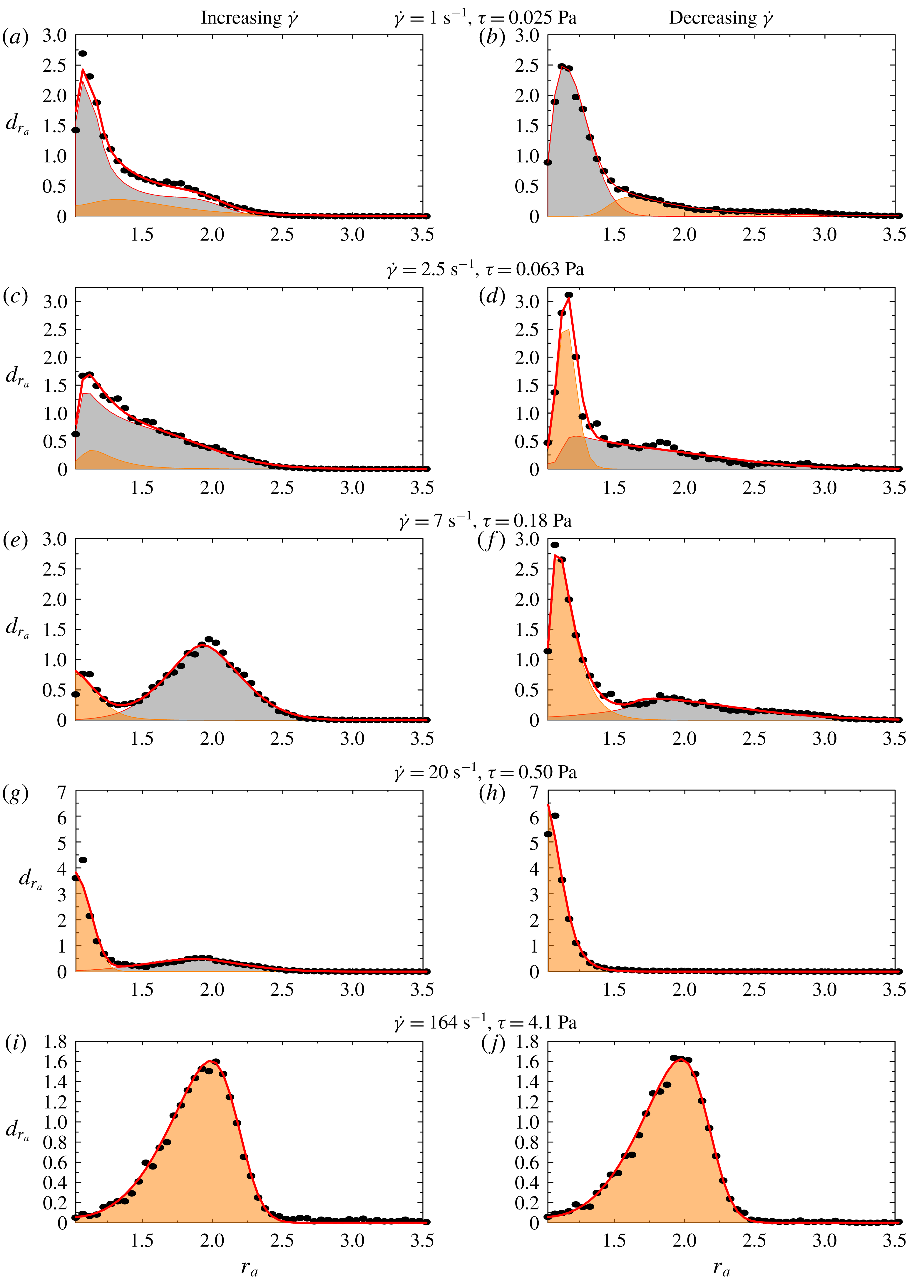
, but in practice it is never larger than 5. Probability densities for
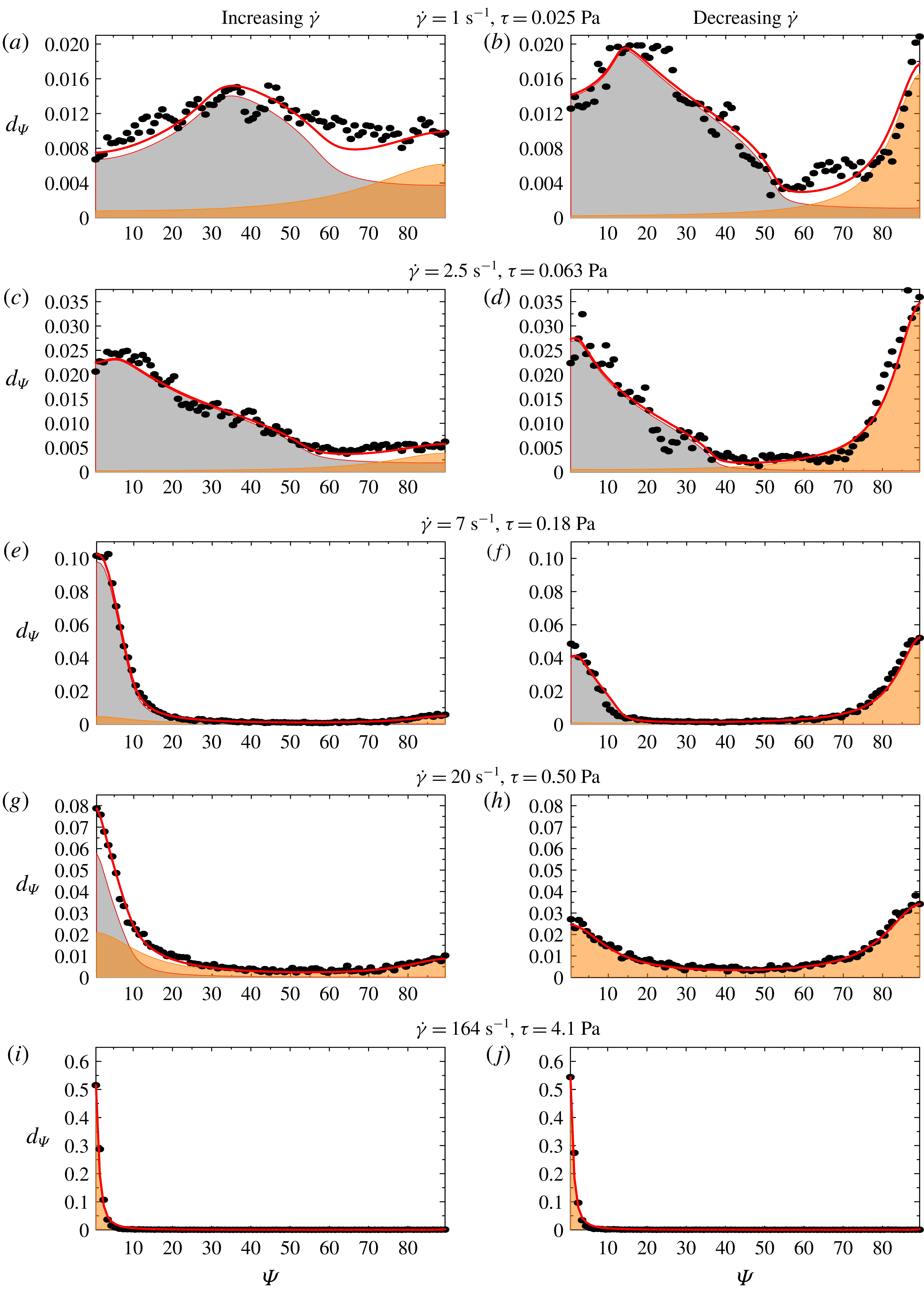
 $\unicode[STIX]{x1D6F9}$
and
 $r_{a}$
are then calculated for each shear rate. For simplicity, we consider the
 $\unicode[STIX]{x1D6F9}$
and
 $r_{a}$
distributions separately, so as to make the fitting procedure described in the next section converge more easily and in a reasonable amount of time. A long computing time is due to the necessity to consider only discrete data sets instead of formal expressions for some fitting functions, as described in the next section. The bin sizes are
 $\unicode[STIX]{x1D6FF}r_{a}=0.05$
for
 $r_{a}$
and
 $\unicode[STIX]{x1D6FF}\unicode[STIX]{x1D6F9}=1^{\circ }$
for
 $\unicode[STIX]{x1D6F9}$
. For high
 $\dot{\unicode[STIX]{x1D6FE}}$
, around 6000 cell pictures are included in the statistics. This number is regularly increased as lower shear rates are considered, up to 40 000 for the lower shear rate
 $0.5~\text{s}^{-1}$
, so as to describe more complex dynamics with many orbit angles accurately. This last number corresponds to about 500 different cells that were observed at least once.
5 Model and data analysis
In this section, the experimental probability densities are compared with the theoretical distribution for
 $\unicode[STIX]{x1D6F9}$
and
 $r_{a}$
that are expected from the model described.
5.1 Premise
We assume that, for a given shear rate, the suspension is composed at each time, on average, of a proportion
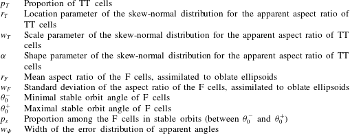
 $p_{T}$
of cells in tank-treading-like (or swinging) motion and a proportion
 $1-p_{T}$
of cells in flipping motion following a Jeffery orbit, where the orbit angle
 $\unicode[STIX]{x1D703}_{0}$
can be between 0 (rolling) and
 $90^{\circ }$
(tumbling). In Dupire et al. (Reference Dupire, Socol and Viallat2012), it is shown that above a threshold value, orbits are unstable and the cells switch from one orbit to another, with angles between this threshold and
 $90^{\circ }$
. In contrast, below this value orbits are stable. In order to explore this idea, we look for two subpopulations of flipping cells: (i) with proportion
 $p_{s}$
, those with stable orbits that we suppose to lie between two extremal values
 $\unicode[STIX]{x1D703}_{0}^{-}$
and
 $\unicode[STIX]{x1D703}_{0}^{+}$
, with equal probability; while this may appear as a strong statement, this is the only reasonable choice amongst the possible distributions that would lead to a reasonable number of fitting parameters; (ii) with proportion
 $(1-p_{s})$
, those with unstable orbits with angles between
 $\unicode[STIX]{x1D703}_{0}^{+}$
and
 $90^{\circ }$
, with equal probability. In addition, shear stress may have an influence on the cells’ aspect ratio, which should also be determined.
In the following, we derive the expression of the theoretical densities that include the geometrical and dynamical characteristics of the tank-treading and flipping regimes, but also the dispersion in size and shape within a sample and the uncertainties associated with the shape characterizations.
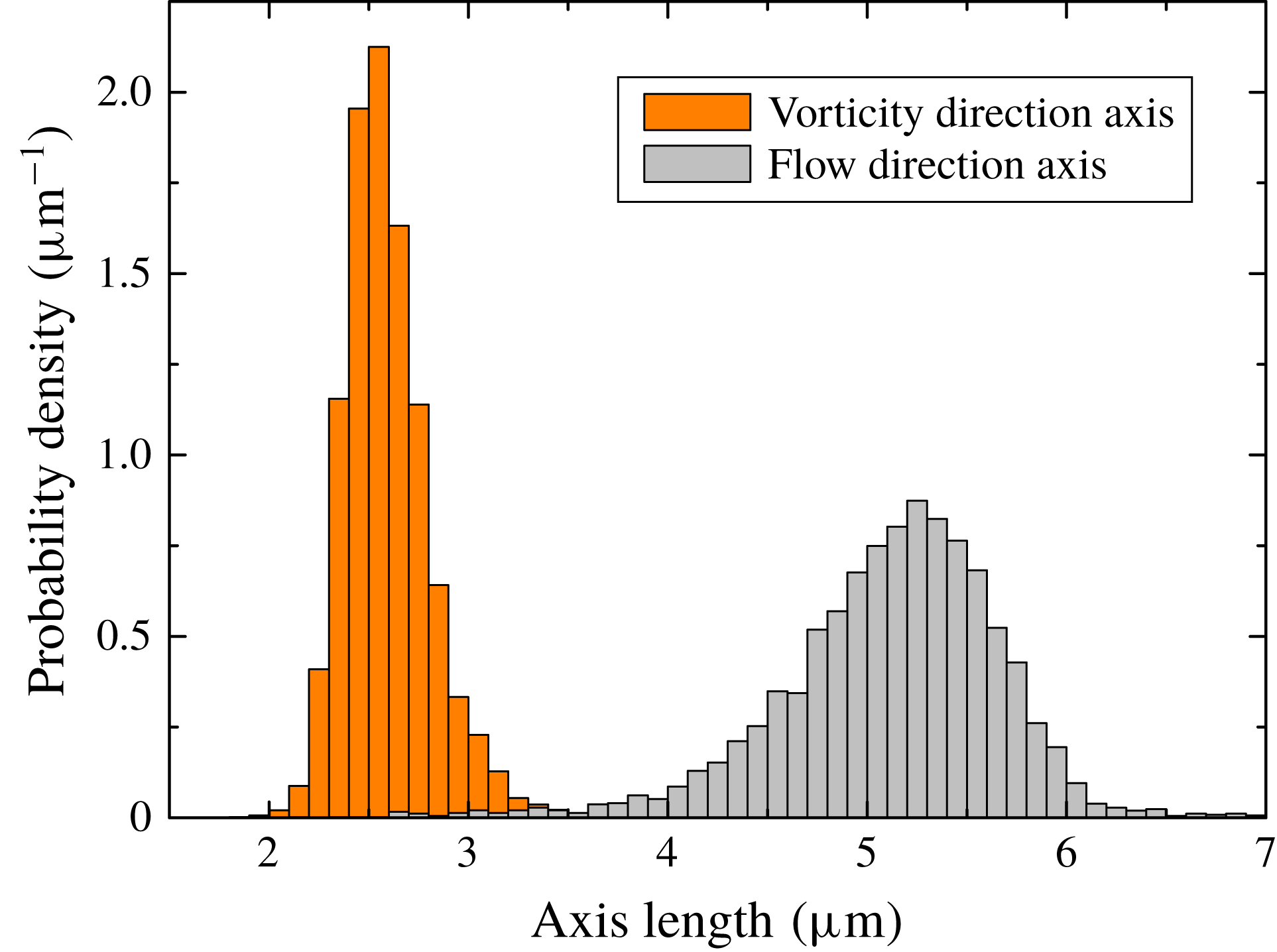
Probability density for the length of the projected shapes of RBCs, in the vorticity and flow direction, in the
 $\unicode[STIX]{x1D702}=25~\text{mPa}~\text{s}$
solution, for
 $\dot{\unicode[STIX]{x1D6FE}}=200~\text{s}^{-1}$
.

5.2 Tank-treading
Viewed from the shear axis direction, depending on the elongation of the cell (increasing with shear rate), but also on its angle
 $\unicode[STIX]{x03C0}/2-\unicode[STIX]{x1D719}$
compared with the flow direction (decreasing with shear rate), a tank-treading (or swinging) cell will appear as an ellipse whose long axis may be in the flow or in the vorticity direction. We therefore look for two populations of cells, in proportion
 $\unicode[STIX]{x1D6FD}$
and
 $1-\unicode[STIX]{x1D6FD}$
, with orientations 0 and
 $90^{\circ }$
. The theoretical distribution
 $d_{\unicode[STIX]{x1D6F9},TT}$
on
 $[0^{\circ };90^{\circ }]$
is then, in principle,
 $$\begin{eqnarray}d_{\unicode[STIX]{x1D6F9},TT}[\unicode[STIX]{x1D6FD}](\unicode[STIX]{x1D6F9})=\unicode[STIX]{x1D6FD}2\unicode[STIX]{x1D6FF}_{0}(\unicode[STIX]{x1D6F9})+(1-\unicode[STIX]{x1D6FD})2\unicode[STIX]{x1D6FF}_{90}(\unicode[STIX]{x1D6F9}),\end{eqnarray}$$
where
 $\unicode[STIX]{x1D6FF}_{\unicode[STIX]{x1D6F9}_{0}}$
is the Dirac distribution centred on
 $\unicode[STIX]{x1D6F9}_{0}$
.
Here and in the following, we place the parameters of the distribution inside square brackets
 $[-]$
while the studied variable is placed inside parentheses
 $(-)$
. For the aspect ratio, we note that the size distribution is large, as at rest: typical range for the long axis of a cell at rest is 7–
 $9~\unicode[STIX]{x03BC}\text{m}$
(see Canham & Burton Reference Canham and Burton1968). In addition, the distribution of apparent cell length in the flow direction is not symmetric but has a shorter tail on the large values side (see figure 5). The distribution of width in the vorticity direction is not symmetric either, with a shorter tail on the low value side. This may be due to many factors: uneven distribution of the deformability among the cells (see Dobbe et al.
Reference Dobbe, Streekstra, Hardeman, Ince and Grimbergen2002b
), saturation of deformation of a given cell under shear (it would not be possible to elongate a cell and shrink it in the vorticity direction beyond a given threshold), a result of swinging dynamics that favours some projected lengths (not valid for width). For the aspect ratio
 $r_{zx}=$
(flow direction axis/vorticity direction axis) we shall therefore expect an asymmetric distribution (see Dobbe et al.
Reference Dobbe, Hardeman, Streekstra, Strackee, Ince and Grimbergen2002a
). It appeared that the skew-normal distribution, defined by
 $$\begin{eqnarray}p_{sG}[r_{T},w_{T},\unicode[STIX]{x1D6FC}](r_{zx})\propto \left(1+\text{erf}\left(\frac{\unicode[STIX]{x1D6FC}(r_{zx}-r_{T})}{\sqrt{2}w_{T}}\right)\right)\text{e}^{-(r_{zx}-r_{T})^{2}/(2w_{T}^{2})},\end{eqnarray}$$
works well. Here
 $\unicode[STIX]{x1D6FC}$
is an asymmetry parameter that will be negative in our case. In our general analysis, we chose to consider the aspect ratio
 $r_{a}$
between the long axis and the short axis of the cells, a parameter that is defined even for cells not parallel or perpendicular to flow. Here, we shall therefore consider the inverse aspect ratio for the cells with aspect ratio
 $r_{zx}$
lower than 1, hence the following theoretical distribution
 $d_{r_{a},TT}$
for
 $r_{a}$
:
 $$\begin{eqnarray}d_{r_{a},TT}[r_{T},w_{T},\unicode[STIX]{x1D6FC}](r_{a})=\unicode[STIX]{x1D6E9}(r_{a}-1)\left[p_{sG}[r_{T},w_{T},\unicode[STIX]{x1D6FC}](r_{a})+\frac{1}{r_{a}^{2}}p_{sG}[r_{T},w_{T},\unicode[STIX]{x1D6FC}]\left(\frac{1}{r_{a}}\right)\right],\end{eqnarray}$$
with
 $\unicode[STIX]{x1D6E9}$
the Heaviside function. The proportion
 $\unicode[STIX]{x1D6FD}$
of cells whose projection is aligned with the flow (5.1), is equal to
 $\int _{1}^{\infty }p_{sG}[r_{T},w_{T},\unicode[STIX]{x1D6FC}](r_{a})\,\text{d}r_{a}$
.
5.3 Flipping motion
Although cells are not exactly ellipsoids, we assume that the dynamics of a flipping cell may still be described by the Jeffery orbit of an ellipsoid having the same aspect ratio
 $r$
as the convex envelope of the cell, as in Anczurowski & Mason (Reference Anczurowski and Mason1967).
In experiments, the optical axis is
 $y^{\prime }$
and we visualize its projection on the
 $x^{\prime }z^{\prime }$
plane (see figure 1 for the notation and figure 2 for an example). The relationship between the coordinates
 $(x,y,z)$
in the moving
 $Oxyz$
coordinate system and
 $(x^{\prime },y^{\prime },z^{\prime })$
in the
 $Ox^{\prime }y^{\prime }z^{\prime }$
coordinate system is, according to the convention used here,
 $$\begin{eqnarray}\left(\begin{array}{@{}c@{}}x\\ y\\ z\end{array}\right)=\left[\left(\begin{array}{@{}ccc@{}}1 & 0 & 0\\ 0 & \cos \unicode[STIX]{x1D719} & -\text{sin}\unicode[STIX]{x1D719}\\ 0 & \sin \unicode[STIX]{x1D719} & \cos \unicode[STIX]{x1D719}\\ \end{array}\right)\left(\begin{array}{@{}ccc@{}}\cos \unicode[STIX]{x1D703} & -\text{sin}\unicode[STIX]{x1D703} & 0\\ \sin \unicode[STIX]{x1D703} & \cos \unicode[STIX]{x1D703} & 0\\ 0 & 0 & 1\\ \end{array}\right)\right]^{-1}\left(\begin{array}{@{}c@{}}x^{\prime }\\ y^{\prime }\\ z^{\prime }\end{array}\right).\end{eqnarray}$$
Equations (2.1) and (5.4) yield the equation of the ellipsoid in the
 $Ox^{\prime }y^{\prime }z^{\prime }$
coordinate system. This is a quadratic equation in
 $x^{\prime }$
,
 $y^{\prime }$
and
 $z^{\prime }$
, with parameters
 $r$
,
 $\unicode[STIX]{x1D703}$
and
 $\unicode[STIX]{x1D719}$
. The contour of the projection of the ellipsoid along the
 $y^{\prime }$
axis corresponds to the
 $x^{\prime }z^{\prime }$
points for which the ellipsoid equation has exactly one solution for
 $y^{\prime }$
. It yields the quadratic equation of an ellipse for
 $x^{\prime }$
and
 $z^{\prime }$
, which can be written as
 $A(r,\unicode[STIX]{x1D703},\unicode[STIX]{x1D719}){x^{\prime }}^{2}+B(r,\unicode[STIX]{x1D703},\unicode[STIX]{x1D719})x^{\prime }z^{\prime }+C(r,\unicode[STIX]{x1D703},\unicode[STIX]{x1D719}){z^{\prime }}^{2}=1$
.
The angle
 $\unicode[STIX]{x1D6F9}$
of the long axis relatively to flow direction
 $z^{\prime }$
and the aspect ratio (long axis/short axis)
 $r_{a}$
of this ellipse are given by
 $$\begin{eqnarray}\displaystyle & \displaystyle \cot \unicode[STIX]{x1D6F9}=(-A+C-\sqrt{(A-C)^{2}+B^{2}})/B, & \displaystyle\end{eqnarray}$$
 $$\begin{eqnarray}\displaystyle & \displaystyle r_{a}=\sqrt{(A+C+\sqrt{(A-C)^{2}+B^{2}})/(A+C-\sqrt{(A-C)^{2}+B^{2}})}. & \displaystyle\end{eqnarray}$$
For a given aspect ratio
 $r$
and orbit parameter
 $\unicode[STIX]{x1D703}_{0}$
we can calculate the trajectories
 $\unicode[STIX]{x1D6F9}(r,\unicode[STIX]{x1D703}_{0},t)$
and
 $r_{a}(r,\unicode[STIX]{x1D703}_{0},t)$
over one period and deduce the associated probability function for
 $\unicode[STIX]{x1D6F9}$
and
 $r_{a}$
, as the probability is inversely proportional to the time derivative of the considered parameter. For
 $r_{a}$
it yields a very complex function, which furthermore has to be integrated to normalize the probability, making the calculation unfeasible. For
 $\unicode[STIX]{x1D6F9}$
, thanks to the more direct (2.6), this can indeed be more easily done, and one finds, for
 $\unicode[STIX]{x1D6F9}$
cast onto
 $[0;90^{\circ }]$
, the probability density
 $$\begin{eqnarray}p_{\unicode[STIX]{x1D6F9}}[\unicode[STIX]{x1D703}_{0}](\unicode[STIX]{x1D6F9})=\frac{1+\tan ^{2}\unicode[STIX]{x1D6F9}}{90\tan \unicode[STIX]{x1D703}_{0}\sqrt{1-\tan ^{2}\unicode[STIX]{x1D6F9}/\tan ^{2}\unicode[STIX]{x1D703}_{0}}}\quad \text{if }\unicode[STIX]{x1D6F9}<\unicode[STIX]{x1D703}_{0},\text{ and 0 otherwise.}\end{eqnarray}$$
Interestingly, for a given
 $\unicode[STIX]{x1D703}_{0}$
, the apparent angle probability does not depend on
 $r$
. This could already be seen from the expression (2.6), where the aspect ratio
 $r$
only appears in the expression through the period.
To calculate the probability density
 $p_{r_{a}}$
for
 $r_{a}$
we chose to sample
 $r_{a}(r,\unicode[STIX]{x1D703}_{0},t)$
given by (5.6) over one period
 $T$
with time step
 $10^{-3}T$
and infer the associated probabilities
 $p_{r_{a}}[r,\unicode[STIX]{x1D703}_{0}](r_{a})$
with bin size 0.05 as for the experimental data, for all aspect ratios
 $r$
between
 $r_{min}=1.025$
and
 $r_{max}=4.975$
with step
 $\unicode[STIX]{x1D6FF}r=0.05$
and all orbit angles
 $\unicode[STIX]{x1D703}_{0}$
between 0 and
 $90^{\circ }$
with step
 $\unicode[STIX]{x1D6FF}\unicode[STIX]{x1D703}_{0}=0.25^{\circ }$
. This set of
 $80\times 361=28\,880$
discretized probability distributions will be used in the fitting procedure.
Following the premise of this modelling section, the expected distributions are eventually obtained by considering that the orbit angle lies between two extremal values
 $\unicode[STIX]{x1D703}_{0}^{-}$
and
 $\unicode[STIX]{x1D703}_{0}^{+}$
, with equal probabilities of sum
 $p_{s}$
or between
 $\unicode[STIX]{x1D703}_{0}^{+}$
and
 $90^{\circ }$
, with equal probabilities of sum
 $(1-p_{s})$
and that, because the cell population is not fully homogeneous, there can be some variation in their aspect ratio. We consider normal
 $p_{G}[r_{F},w_{F}](r)$
distribution for the cell aspect ratio (see Rodak, Fritsma & Doig Reference Rodak, Fritsma and Doig2007), with mean
 $r_{F}$
and standard deviation
 $w_{F}$
. We would thus seek a
 $\unicode[STIX]{x1D6F9}$
and
 $r_{a}$
distribution in the flipping regime
 $$\begin{eqnarray}\displaystyle & & \displaystyle d_{r_{a},F}[r_{F},w_{F},\unicode[STIX]{x1D703}_{0}^{-},\unicode[STIX]{x1D703}_{0}^{+},p_{s}](r_{a})=\mathop{\sum }_{r=r_{min}}^{r_{max}}p_{G}[r_{F},w_{F}](r)\unicode[STIX]{x1D6FF}r\nonumber\\ \displaystyle & & \displaystyle \quad \times \left(\frac{p_{s}\unicode[STIX]{x1D6FF}\unicode[STIX]{x1D703}_{0}}{\unicode[STIX]{x1D703}_{0}^{+}-\unicode[STIX]{x1D703}_{0}^{-}+\unicode[STIX]{x1D6FF}\unicode[STIX]{x1D703}_{0}}\mathop{\sum }_{\unicode[STIX]{x1D703}_{0}=\unicode[STIX]{x1D703}_{0}^{-}}^{\unicode[STIX]{x1D703}_{0}^{+}}p_{r_{a}}[r,\unicode[STIX]{x1D703}_{0}](r_{a})+\frac{(1-p_{s})\unicode[STIX]{x1D6FF}\unicode[STIX]{x1D703}_{0}}{90-\unicode[STIX]{x1D703}_{0}^{+}+\unicode[STIX]{x1D6FF}\unicode[STIX]{x1D703}_{0}}\mathop{\sum }_{\unicode[STIX]{x1D703}_{0}=\unicode[STIX]{x1D703}_{0}^{-}}^{90}p_{r_{a}}[r,\unicode[STIX]{x1D703}_{0}](r_{a})\right),\qquad\end{eqnarray}$$
 $$\begin{eqnarray}d_{\unicode[STIX]{x1D6F9},F}[\unicode[STIX]{x1D703}_{0}^{-},\unicode[STIX]{x1D703}_{0}^{+},p_{s}](\unicode[STIX]{x1D6F9})=\frac{p_{s}\unicode[STIX]{x1D6FF}\unicode[STIX]{x1D703}_{0}}{\unicode[STIX]{x1D703}_{0}^{+}-\unicode[STIX]{x1D703}_{0}^{-}+\unicode[STIX]{x1D6FF}\unicode[STIX]{x1D703}_{0}}\mathop{\sum }_{\unicode[STIX]{x1D703}_{0}=\unicode[STIX]{x1D703}_{0}^{-}}^{\unicode[STIX]{x1D703}_{0}^{+}}p_{\unicode[STIX]{x1D6F9}}[\unicode[STIX]{x1D703}_{0}](\unicode[STIX]{x1D6F9})+\frac{(1-p_{s})\unicode[STIX]{x1D6FF}\unicode[STIX]{x1D703}_{0}}{90-\unicode[STIX]{x1D703}_{0}^{+}+\unicode[STIX]{x1D6FF}\unicode[STIX]{x1D703}_{0}}\mathop{\sum }_{\unicode[STIX]{x1D703}_{0}=\unicode[STIX]{x1D703}_{0}^{+}}^{90}p_{\unicode[STIX]{x1D6F9}}[\unicode[STIX]{x1D703}_{0}](\unicode[STIX]{x1D6F9}).\end{eqnarray}$$
Sums on
 $r$
are made with step
 $\unicode[STIX]{x1D6FF}r$
and sums on
 $\unicode[STIX]{x1D703}_{0}$
use step
 $\unicode[STIX]{x1D6FF}\unicode[STIX]{x1D703}_{0}$
. Both steps are those used for the generation of the reference distributions.
5.4 Error function on angles
Experimental uncertainty on aspect ratio determination is considered by the use of (skew-)normal distributions.
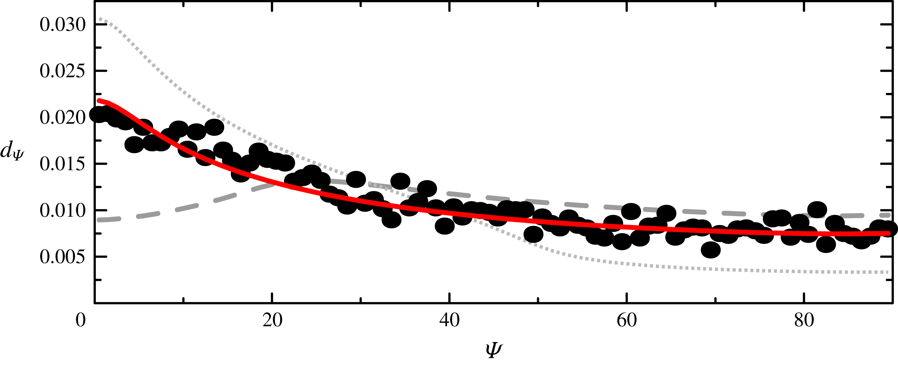
The determination of the cell angle may lead to huge errors when the cell apparent aspect ratio is close to 1. If one considers the ellipse equation
 $Ax^{2}+Bxz+Cz^{2}=1$
with
 $A$
,
 $B$
and
 $C$
being normally distributed around
 $1$
,
 $0$
and
 $1+\unicode[STIX]{x1D716}$
, respectively, and variances of the order of 0.1 close to the experimental ones, one numerically finds an orientation angle distribution that is centred on 0 but with a long tail such that it is rather well described by a Cauchy distribution. As the considered angles are in the interval
 $[0;90]$
we will therefore consider, instead of
 $\unicode[STIX]{x1D6FF}$
functions, the Cauchy distribution folded onto this interval:
 $$\begin{eqnarray}\tilde{p}_{C}[\unicode[STIX]{x1D6F9}_{0},w_{\unicode[STIX]{x1D6F9}}](\unicode[STIX]{x1D6F9})=p_{C}[\unicode[STIX]{x1D6F9}_{0},w_{\unicode[STIX]{x1D6F9}}](\unicode[STIX]{x1D6F9})+p_{C}[\unicode[STIX]{x1D6F9}_{0},w_{\unicode[STIX]{x1D6F9}}](-\unicode[STIX]{x1D6F9})+p_{C}[\unicode[STIX]{x1D6F9}_{0},w_{\unicode[STIX]{x1D6F9}}](180-\unicode[STIX]{x1D6F9}),\end{eqnarray}$$
with
 $p_{C}[\unicode[STIX]{x1D6F9}_{0},w_{\unicode[STIX]{x1D6F9}}](\unicode[STIX]{x1D6F9})=1/(w_{\unicode[STIX]{x1D6F9}}\unicode[STIX]{x03C0}(1+((\unicode[STIX]{x1D6F9}-\unicode[STIX]{x1D6F9}_{0})^{2})/w_{\unicode[STIX]{x1D6F9}}^{2}))$
the Cauchy distribution function around
 $\unicode[STIX]{x1D6F9}_{0}$
.
For the tank-treading regime, we will thus consider the modified distribution function for the angle:
 $$\begin{eqnarray}\hat{d}_{\unicode[STIX]{x1D6F9},TT}[\unicode[STIX]{x1D6FD},w_{\unicode[STIX]{x1D6F9}}](\unicode[STIX]{x1D6F9})=\unicode[STIX]{x1D6FD}\tilde{p}_{C}[0,w_{\unicode[STIX]{x1D6F9}}](\unicode[STIX]{x1D6F9})+(1-\unicode[STIX]{x1D6FD})\tilde{p}_{C}[90,w_{\unicode[STIX]{x1D6F9}}](\unicode[STIX]{x1D6F9}).\end{eqnarray}$$
Here
 $w_{\unicode[STIX]{x1D6F9}}$
is a free parameter that is expected to increase when
 $\dot{\unicode[STIX]{x1D6FE}}$
decreases, to take into account the fact that the aspect ratio approaches 1.
For the flipping cells, the link between aspect ratio and angle is more complex. The apparent aspect ratio is maximal when
 $\unicode[STIX]{x1D6F9}=\unicode[STIX]{x1D703}_{0}$
(cell viewed from the edge,
 $\unicode[STIX]{x1D719}=\pm 90^{\circ }$
). It is minimal when
 $\unicode[STIX]{x1D6F9}=0$
, but this minimal value depends on the orbit: it reaches 1 only for tumbling (
 $\unicode[STIX]{x1D703}_{0}=90^{\circ }$
). Therefore, the uncertainty on a given angle depends on the orbit the cell is following. Thus, to continue handling the
 $r_{a}$
distribution and the
 $\unicode[STIX]{x1D6F9}$
distribution separately, we make the simplifying assumption that, for a given orbit, the width of the modified Cauchy function is 0 when the angle is equal to its maximum value
 $\unicode[STIX]{x1D703}_{0}$
and increases linearly with the distance between the angle and the orbit angle. We, thus, consider the modified distribution for one orbit:
 $$\begin{eqnarray}\hat{p}_{\unicode[STIX]{x1D6F9}}[\unicode[STIX]{x1D703}_{0},w_{\unicode[STIX]{x1D6F9}}](\unicode[STIX]{x1D6F9})=\mathop{\sum }_{\unicode[STIX]{x1D709}=0}^{90}p_{\unicode[STIX]{x1D6F9}}[\unicode[STIX]{x1D703}_{0}](\unicode[STIX]{x1D709})\tilde{p}_{C}[\unicode[STIX]{x1D709},w_{\unicode[STIX]{x1D6F9}}|\unicode[STIX]{x1D709}-\unicode[STIX]{x1D703}_{0}|/90](\unicode[STIX]{x1D6F9}).\end{eqnarray}$$
Here,
 $w_{\unicode[STIX]{x1D6F9}}$
is the width of the error distribution when the aspect ratio is close to 1 (
 $\unicode[STIX]{x1D703}_{0}=90^{\circ }$
,
 $\unicode[STIX]{x1D709}=0$
). For simplicity, we shall consider the same
 $w_{\unicode[STIX]{x1D6F9}}$
for both tank-treading and flipping distributions. Both tank-treading and flipping populations will coexist in the highly viscous solution. At high shear rate, tank-treading cells have aspect ratio far from 1 so
 $w_{\unicode[STIX]{x1D6F9}}$
will be smaller than the expected value for the flipping cells, but in that case, there are few of latter. As
 $\dot{\unicode[STIX]{x1D6FE}}$
decreases, flipping cells will appear but in the meantime the apparent aspect ratio of tank-treading cells will be close to 1, and the
 $w_{\unicode[STIX]{x1D6F9}}$
values should coincide reasonably.
Finally, the modified distribution function for the flipping regime is
 $$\begin{eqnarray}\displaystyle \hat{d}_{\unicode[STIX]{x1D6F9},F}[\unicode[STIX]{x1D703}_{0}^{-},\unicode[STIX]{x1D703}_{0}^{+},p_{s},w_{\unicode[STIX]{x1D6F9}}](\unicode[STIX]{x1D6F9}) & = & \displaystyle \frac{p_{s}\unicode[STIX]{x1D6FF}\unicode[STIX]{x1D703}_{0}}{\unicode[STIX]{x1D703}_{0}^{+}-\unicode[STIX]{x1D703}_{0}^{-}+\unicode[STIX]{x1D6FF}\unicode[STIX]{x1D703}_{0}}\mathop{\sum }_{\unicode[STIX]{x1D703}_{0}=\unicode[STIX]{x1D703}_{0}^{-}}^{\unicode[STIX]{x1D703}_{0}^{+}}\hat{p}_{\unicode[STIX]{x1D6F9}}[\unicode[STIX]{x1D703}_{0},w_{\unicode[STIX]{x1D6F9}}](\unicode[STIX]{x1D6F9})\nonumber\\ \displaystyle & & \displaystyle +\,\frac{(1-p_{s})\unicode[STIX]{x1D6FF}\unicode[STIX]{x1D703}_{0}}{90-\unicode[STIX]{x1D703}_{0}^{+}+\unicode[STIX]{x1D6FF}\unicode[STIX]{x1D703}_{0}}\mathop{\sum }_{\unicode[STIX]{x1D703}_{0}=\unicode[STIX]{x1D703}_{0}^{+}}^{90}\hat{p}_{\unicode[STIX]{x1D6F9}}[\unicode[STIX]{x1D703}_{0},w_{\unicode[STIX]{x1D6F9}}](\unicode[STIX]{x1D6F9}).\end{eqnarray}$$
5.5 Complete fitting function
Considering that we have two populations of cells, one in tank-treading-like regime with proportion
 $p_{T}$
and one in flipping regime in proportion
 $(1-p_{T})$
, we finally have the following fitting functions for the distributions in apparent aspect ratio
 $r_{a}$
and apparent angle
 $\unicode[STIX]{x1D6F9}$
, respectively, defined on
 $[1;+\infty ]$
and
 $[0;90]$
, with 10 fitting parameters:
 $$\begin{eqnarray}\displaystyle & & \displaystyle d_{r_{a}}[p_{T},r_{T},w_{T},\unicode[STIX]{x1D6FC},r_{F},w_{F},\unicode[STIX]{x1D703}_{0}^{-},\unicode[STIX]{x1D703}_{0}^{+},p_{s}](r_{a})\nonumber\\ \displaystyle & & \displaystyle \quad =p_{T}d_{r_{a},TT}[r_{T},w_{T},\unicode[STIX]{x1D6FC}](r_{a})+(1-p_{T})d_{r_{a},F}[r_{F},w_{F},\unicode[STIX]{x1D703}_{0}^{-},\unicode[STIX]{x1D703}_{0}^{+},p_{s}](r_{a}),\end{eqnarray}$$
with
 $d_{r_{a},TT}$
given by (5.3) and
 $d_{r_{a},F}$
by (5.8), and
 $$\begin{eqnarray}\displaystyle & & \displaystyle d_{\unicode[STIX]{x1D6F9}}[p_{T},r_{T},w_{T},\unicode[STIX]{x1D6FC},\unicode[STIX]{x1D703}_{0}^{-},\unicode[STIX]{x1D703}_{0}^{+},p_{s},w_{\unicode[STIX]{x1D713}}](\unicode[STIX]{x1D6F9})\nonumber\\ \displaystyle & & \displaystyle \quad =p_{T}\hat{d}_{\unicode[STIX]{x1D6F9},TT}[\unicode[STIX]{x1D6FD},w_{\unicode[STIX]{x1D6F9}}](\unicode[STIX]{x1D6F9})+(1-p_{T})\hat{d}_{\unicode[STIX]{x1D6F9},F}[\unicode[STIX]{x1D703}_{0}^{-},\unicode[STIX]{x1D703}_{0}^{+},p_{s},w_{\unicode[STIX]{x1D6F9}}](\unicode[STIX]{x1D6F9}),\nonumber\\ \displaystyle & & \displaystyle \qquad \quad \text{with }\unicode[STIX]{x1D6FD}=\int _{1}^{\infty }p_{sG}[r_{T},w_{T},\unicode[STIX]{x1D6FC}](r_{a})\,\text{d}r_{a}.\end{eqnarray}$$
Here
 $\hat{d}_{\unicode[STIX]{x1D6F9},TT}$
is given by (5.11) and
 $\hat{d}_{\unicode[STIX]{x1D6F9},F}$
by (5.13).
The fitting parameters are recalled in table 1. For each shear rate, we minimize the distance between the theoretical and experimental distribution functions for
 $r_{a}$
and
 $\unicode[STIX]{x1D6F9}$
, given by
 $$\begin{eqnarray}\displaystyle \unicode[STIX]{x1D716} & = & \displaystyle \mathop{\sum }_{\unicode[STIX]{x1D6F9}}|d_{\unicode[STIX]{x1D6F9},exp}(\unicode[STIX]{x1D6F9})-d_{\unicode[STIX]{x1D6F9}}[p_{T},r_{T},w_{T},\unicode[STIX]{x1D6FC},\unicode[STIX]{x1D703}_{0}^{-},\unicode[STIX]{x1D703}_{0}^{+},p_{s},w_{\unicode[STIX]{x1D713}}](\unicode[STIX]{x1D6F9})|\unicode[STIX]{x1D6FF}\unicode[STIX]{x1D6F9}\nonumber\\ \displaystyle & & \displaystyle +\,\mathop{\sum }_{r_{a}}|d_{r_{a},exp}(r_{a})-d_{r_{a}}[p_{T},r_{T},w_{T},\unicode[STIX]{x1D6FC},r_{F},w_{F},\unicode[STIX]{x1D703}_{0}^{-},\unicode[STIX]{x1D703}_{0}^{+},p_{s}](r_{a})|\unicode[STIX]{x1D6FF}r_{a}.\end{eqnarray}$$
Because they appear as bounds in sums, the parameters
 $\unicode[STIX]{x1D703}_{0}^{-}$
and
 $\unicode[STIX]{x1D703}_{0}^{+}$
are treated differently from the other parameters. For a given choice of these angles, we minimize
 $\unicode[STIX]{x1D716}$
using the NMinimize function of Mathematica© software. We then explore systematically the region of interest for these angles so as to find the global minimum.
6 Results
6.1 Preliminary result: hardened cells
Glutaraldehyde-hardened cells were studied at
 $\dot{\unicode[STIX]{x1D6FE}}=200~\text{s}^{-1}$
in the
 $\unicode[STIX]{x1D702}_{0}=1.5~\text{mPa}~\text{s}$
solution. No tank-treading motion is expected and we find that the apparent angle distribution is fully compatible with that of flipping cells with orbit angles equally distributed in the
 $[0^{\circ };90^{\circ }]$
interval, as shown in figure 6. This is agreement with the fact that Jeffery orbits are stable at low Reynolds number: the followed orbit only depends on the initial condition.

Apparent angle
 $\unicode[STIX]{x1D6F9}$
probability distribution for hardened cells in the suspending medium of viscosity 1.5 mPa s, for different
 $\dot{\unicode[STIX]{x1D6FE}}=200~\text{s}^{-1}$
. Dots: experimental data; red solid line: full fit (5.15) with
 $p_{T}=0$
(no tank-treading cells),
 $\unicode[STIX]{x1D703}_{0}^{-}=0^{\circ }$
,
 $\unicode[STIX]{x1D703}_{0}^{+}=90^{\circ }$
. In order to help understand more complex distributions, we also show the distribution for
 $\unicode[STIX]{x1D703}_{0}^{-}=20^{\circ }$
, that exhibits a peak around
 $20^{\circ }$
(dotted line), and a case where the probability of orbits between
 $50^{\circ }$
and
 $90^{\circ }$
is
 $1/4$
of that between
 $0^{\circ }$
and
 $50^{\circ }$
(dashed line). A strong decrease can be seen around
 $50^{\circ }$
.

Selection of apparent angle
 $\unicode[STIX]{x1D6F9}$
probability distributions for cells in the suspending medium of viscosity 25 mPa s, for different shear rates. Dots: experimental data; red line: full fit (5.15); orange line and area: tank-treading population; red line and grey area: flipping population.

Selection of apparent aspect ratio
 $r_{a}$
probability distributions for cells in the suspending medium of viscosity 25 mPa s, for different shear rates. Dots: experimental data; red line: full fit (5.14); orange line and area: tank-treading population; red line and grey area: flipping population.

6.2 Cells in fluid of high viscosity
6.2.1 Examples of fits
We first comment on a set of fits obtained in the
 $\unicode[STIX]{x1D702}_{0}=25~\text{mPa}~\text{s}$
case for selected shear rates (see figures 7 and 8), so as to validate the modelling hypotheses and draw a rough scenario for cell dynamics. At high shear rates (
 $\dot{\unicode[STIX]{x1D6FE}}=164~\text{s}^{-1}$
and higher values), it is known that all cells are in the tank-treading regime. The apparent aspect ratio distribution is well described by the proposed skew-normal distribution (figure 8
i,j), whereas all angles are close to zero due to strong cell elongation (figure 7
i,j). The width
 $w_{\unicode[STIX]{x1D6F9}}$
of the angle distribution is of order
 $1^{\circ }$
; as the angle determination is quite precise due to the high apparent aspect ratio, this is an indicator of experimental intrinsic fluctuations: shear chamber vibrations and the influence of other cells, which can therefore be considered negligible.
For
 $\dot{\unicode[STIX]{x1D6FE}}=20~\text{s}^{-1}$
, the scenario is different depending on whether
 $\dot{\unicode[STIX]{x1D6FE}}$
is increasing or decreasing. In the latter case, there is still only one population of tank-treading cells, but as the cells are less stretched, their apparent aspect ratio is close to 1. As a consequence, the distribution of their apparent angle has two peaks around 0 and
 $90^{\circ }$
, well described by the proposed Cauchy distribution. The two peaks have almost the same height, indicating an aspect ratio close to 1 (as seen on the
 $r_{a}$
distribution), which is the worst case for angle detection. This results in the presence of all angles in the experimental distribution, which would not be well described by a Gaussian distribution, for instance.
On the other hand, in the increasing
 $\dot{\unicode[STIX]{x1D6FE}}$
case, a second peak appears in the apparent aspect ratio distribution, around
 $r_{a}=2$
, which is more important for
 $\dot{\unicode[STIX]{x1D6FE}}=12~\text{s}^{-1}$
or
 $7~\text{s}^{-1}$
, and corresponds to flipping cells with orbit angles close to
 $0^{\circ }$
, that is, to rolling. This second peak is well fitted by a normal distribution, as hypothesized for (5.8). This second peak of rolling cells is present in the decreasing
 $\dot{\unicode[STIX]{x1D6FE}}$
case, but has lower weight. We shall return to this later.
At low shear rates (
 $\dot{\unicode[STIX]{x1D6FE}}=2.5~\text{s}^{-1}$
and
 $1~\text{s}^{-1}$
for this example), the tank-treading cells contribute in the
 $r_{a}$
distribution with a peak which is now far from 1, with apparent angle is now only around
 $90^{\circ }$
, along the vorticity direction due to the projection. On the other hand, the contribution of flipping cells is more complex because other orbit angles have appeared. This results in a broadening of angle distribution towards higher angles (from 0 to around
 $\unicode[STIX]{x1D703}_{0}^{+}$
), while the aspect ratio distribution broadens towards
 $r_{a}=1$
: flipping cells with
 $\unicode[STIX]{x1D703}_{0}=0$
are always seen from their edge so the apparent aspect ratio is a peak centred on their 3D aspect ratio
 $r$
, while cells with larger
 $\unicode[STIX]{x1D703}_{0}$
also exhibit apparent aspect ratios lower than
 $r$
. Only for
 $\unicode[STIX]{x1D703}_{0}=90^{\circ }$
can this apparent aspect ratio be 1. At the minimum shear rate presented in this example, one can see that the peak of the distribution is no longer located at
 $0^{\circ }$
. As exemplified by the dashed line in figure 6, the location of this peak is indeed an indicator of the value of
 $\unicode[STIX]{x1D703}_{0}^{-}$
. For instance, at
 $\dot{\unicode[STIX]{x1D6FE}}=1~\text{s}^{-1}$
, decreasing case,
 $\unicode[STIX]{x1D703}_{0}^{-}$
is around
 $20^{\circ }$
while
 $\unicode[STIX]{x1D703}_{0}^{+}$
is around
 $50^{\circ }$
.
In particular, in the increasing case, for
 $\dot{\unicode[STIX]{x1D6FE}}=1~\text{s}^{-1}$
and
 $2.5~\text{s}^{-1}$
, the angle distribution does not drop to zero for high angles. This cannot be associated only with tank-treading cells with angle
 $90^{\circ }$
: a look at the probability distribution in the
 $(\unicode[STIX]{x1D6F9},r_{a})$
space (figure 9
a) shows that cells with high angles also have apparent aspect ratios as high as those with low angles; that is, they are also seen edge-on sometimes. This is even clearer when one compares with a case where the high angle cells are in tank-treading regime: in figure 9(b), the aspect ratios of the high angle cells are lower than those of the low angle rolling cells. Note that what matters here is the comparison between the low and high angle populations, not the absolute values of the aspect ratios, that depend on the shear rate through cell deformation. On the other hand, the angle distribution cannot be described by an equal orbit distribution between
 $\unicode[STIX]{x1D703}_{0}^{-}$
and
 $90^{\circ }$
. It requires the population of flipping cells to be divided into two subpopulations, in proportion
 $p_{s}$
and
 $1-p_{s}$
, having orbits between
 $\unicode[STIX]{x1D703}_{0}^{-}$
and
 $\unicode[STIX]{x1D703}_{0}^{+}$
, and
 $\unicode[STIX]{x1D703}_{0}^{+}$
and
 $90^{\circ }$
, respectively, such that the high angle orbits are less probable. This is exemplified by the dotted line in figure 6, to be compared with the solid line corresponding to equal probabilities. For instance, for
 $\dot{\unicode[STIX]{x1D6FE}}=1~\text{s}^{-1}$
, increasing shear rate case, we find
 $p_{s}=0.81$
such that the ratio
 $\unicode[STIX]{x1D6FC}_{u/s}$
between the probability of an orbit with
 $\unicode[STIX]{x1D703}_{0}^{+}<\unicode[STIX]{x1D703}_{0}<90^{\circ }$
, and of that of an orbit with
 $\unicode[STIX]{x1D703}_{0}^{-}<\unicode[STIX]{x1D703}_{0}<\unicode[STIX]{x1D703}_{0}^{+}$
, is equal here to 0.22. Here
 $\unicode[STIX]{x1D6FC}_{u/s}$
is defined by
 $[(1-p_{s})/(90-\unicode[STIX]{x1D703}_{0}^{+})]/[p_{s}/(\unicode[STIX]{x1D703}_{0}^{+}-\unicode[STIX]{x1D703}_{0}^{-})]$
.
Maps of probability densities in the
 $(\unicode[STIX]{x1D6F9},r_{a})$
space: (a)
 $\unicode[STIX]{x1D702}_{0}=25~\text{mPa}~\text{s}$
and
 $\dot{\unicode[STIX]{x1D6FE}}=1~\text{s}^{-1}$
, increasing shear rate case; (b)
 $\unicode[STIX]{x1D702}_{0}=25~\text{mPa}~\text{s}$
and
 $\dot{\unicode[STIX]{x1D6FE}}=7~\text{s}^{-1}$
, decreasing shear rate case.

Main parameters characterizing cell dynamics for
 $\unicode[STIX]{x1D702}_{0}=25~\text{mPa}~\text{s}$
as a function of shear stress
 $\unicode[STIX]{x1D70F}=\unicode[STIX]{x1D702}_{0}\dot{\unicode[STIX]{x1D6FE}}$
in both increasing
 $\dot{\unicode[STIX]{x1D6FE}}$
(full triangles) and decreasing
 $\dot{\unicode[STIX]{x1D6FE}}$
(empty triangles) cases, as indicated by arrows. Empty circles: additional control experiments at decreasing
 $\dot{\unicode[STIX]{x1D6FE}}$
made with RBCs from two other donors and a suspending medium prepared independently. On top of panel (a), the transition between the two stresses indicated by stars corresponds to that studied in figure 16. (a) Proportion
 $p_{T}$
of cells in tank-treading-like motion. (b) Mean apparent aspect ratio
 $\langle r_{zx}\rangle _{T}=r_{T}+w_{T}\unicode[STIX]{x1D6FC}\sqrt{2}/\sqrt{\unicode[STIX]{x03C0}(1+\unicode[STIX]{x1D6FC}^{2})}$
of tank-treading cells. (c) Minimal and maximal orbit angles
 $\unicode[STIX]{x1D703}_{0}^{-}$
and
 $\unicode[STIX]{x1D703}_{0}^{+}$
for stable flipping cells. Dotted symbols indicate the limit orbits (
 $90^{\circ }$
) of (probably) unstable orbits between
 $\unicode[STIX]{x1D703}_{0}^{+}$
and
 $90^{\circ }$
, when present. (d) Ratio
 $\unicode[STIX]{x1D6FC}_{u/s}$
between the probability of orbits with orbit angle between
 $\unicode[STIX]{x1D703}_{0}^{+}$
and
 $90^{\circ }$
, and between
 $\unicode[STIX]{x1D703}_{0}^{-}$
and
 $\unicode[STIX]{x1D703}_{0}^{+}$
.

6.2.2 Transition scenario
In figure 10 we show the evolution with flow stress
 $\unicode[STIX]{x1D70F}=\unicode[STIX]{x1D702}_{0}\dot{\unicode[STIX]{x1D6FE}}$
of the main parameters characterizing the collective dynamics of RBCs.
The main difference between the increasing and the decreasing
 $\dot{\unicode[STIX]{x1D6FE}}$
cases lies in the proportion
 $p_{T}$
of cells in the tank-treading regime (figure 10
a). A full hysteresis loop is highlighted: at low and high flow stresses, the amount of cells in tank-treading regime are identical. At low flow stress, we observe that, according to our model, the proportion of tank-treading cells is not equal to 0. We shall propose later an interpretation of this result, which calls for a refinement of the model.
For increasing
 $\dot{\unicode[STIX]{x1D6FE}}$
, a significant increase in the proportion of tank-treading cells is observed from
 $\unicode[STIX]{x1D70F}_{c-min}^{{>}}=0.08~\text{Pa}$
until all cells are in tank-treading regimes at
 $\unicode[STIX]{x1D70F}_{c-max}^{{>}}=2~\text{Pa}$
. This shows that the dispersion in the transition stress towards tank-treading
 $\unicode[STIX]{x1D70F}_{c}^{{>}}$
is high: the transition values span over one decade. This result is in agreement with Fischer & Korzeniewski (Reference Fischer and Korzeniewski2013), where for
 $\unicode[STIX]{x1D702}_{0}=24~\text{mPa}~\text{s}$
a transition to tank-treading is found around
 $\unicode[STIX]{x1D70F}=0.23~\text{Pa}$
but with a smooth transition that indeed spans over one decade, as here (see figure 2b in Fischer & Korzeniewski (Reference Fischer and Korzeniewski2013)).
For decreasing
 $\dot{\unicode[STIX]{x1D6FE}}$
, the first cells to leave the tank-treading regime do it at a flow stress
 $\unicode[STIX]{x1D70F}_{c-max}^{{<}}=0.4~\text{Pa}$
smaller than
 $\unicode[STIX]{x1D70F}_{c-max}^{{>}}$
. The last cells to leave the tank-treading regime seem to do it around
 $\unicode[STIX]{x1D70F}_{c-min}^{{<}}=0.02~\text{Pa}$
. The values for
 $\unicode[STIX]{x1D70F}_{c}^{{>}}$
and
 $\unicode[STIX]{x1D70F}_{c}^{{<}}$
found in Dupire et al. (Reference Dupire, Socol and Viallat2012) and Mauer et al. (Reference Mauer, Mendez, Lanotte, Nicoud, Abkarian, Gompper and Fedosov2018) lie in the lower part of the transition zone we find.
Figure 10(b) shows the mean aspect ratio of cells in tank-treading regime, considering the aspect ratio
 $r_{zx}$
between the axis along the flow direction and the axis in the vorticity direction, whose distribution is given by (5.2). This mean value is a function of the fit parameters through
 $\langle r_{zx}\rangle _{T}=r_{T}+w_{T}\unicode[STIX]{x1D6FC}\sqrt{2}/\sqrt{\unicode[STIX]{x03C0}(1+\unicode[STIX]{x1D6FC}^{2})}$
and is directly linked to the deformability of cells. Owing to the dispersion in cell properties (and, probably, to swinging motion), the standard deviation around this mean value is between 0.1 and 0.15 within the whole stress range.
Deformation is quite similar for both directions of shear rate variation. However, in the hysteretic region for the tank-treading population, the apparent aspect ratio is up to 10 % smaller in the decreasing
 $\dot{\unicode[STIX]{x1D6FE}}$
case and is almost constant, while it varies more strongly for higher stress values. On the other hand, in this range stress is not so small that we should expect cell shape not to be modified by the flow. Indeed, even for lower stresses transitions between different regimes occur and orbit angles of the flipping regimes change continuously: another explanation for this plateau has to be found.
We note that, while the aspect ratio of cells in the tank-treading regime should be an increasing function of stress, the population of cells in that regime is not constant. We hypothesize that the plateauing shows that, upon an increase of shear rate, the contribution of the cells switching to tank-treading compensates for the increased deformation of the cells already in the tank-treading regime. This implies that the latter are more deformable (in the sense of stretchable) than the newcomers, which are themselves the most deformable of the flipping cells that have not yet switched to tank-treading. This is coherent with the picture of more deformable cells needing smaller stress to make their transition. Similar reasoning shows that, upon a decrease of shear rate, the less deformable cells of the tank treading population are the first to transit towards the flipping motion.
A consequence of this would be that at a given stress, because of the hysteresis in the transition thresholds, the tank-treading population in the decreasing
 $\dot{\unicode[STIX]{x1D6FE}}$
case contains more cells than in the increasing
 $\dot{\unicode[STIX]{x1D6FE}}$
case. To validate the whole picture, let us first denote by
 $P_{T{\nearrow}}$
and
 $P_{T{\searrow}}$
the proportion of cells in the tank-treading regime in the increasing and decreasing
 $\dot{\unicode[STIX]{x1D6FE}}$
cases, respectively. From the previous discussion, we conclude that, among the tank-treading cells in the decreasing
 $\dot{\unicode[STIX]{x1D6FE}}$
case, the more deformable ones are also in the tank-treading regime in the increasing shear rate case, while the less deformable are not. The proportions of these two subpopulations are, by definition,
 $P_{T{\nearrow}}/P_{T{\searrow}}$
and
 $1-P_{T{\nearrow}}/P_{T{\searrow}}$
, respectively. Considering, for a given stress
 $\unicode[STIX]{x1D70F}$
, the whole skew-normal distribution of
 $r_{zx}$
in the decreasing shear rate case, we make a cut-off in this distribution by considering only the last
 $P_{T{\nearrow}}/P_{T{\searrow}}$
cells, on which the mean value of
 $r_{zx}$
, that we denote by
 $\langle r_{zx}\rangle _{T}^{\ast }$
, is calculated. The result is shown in figure 11. The curve of the mean value taken on the more deformable cells in the decreasing shear rate case now collapses onto the mean value
 $\langle r_{zx}\rangle _{T}$
in the increasing shear rate case, thus validating our hypothesis.
Mean apparent aspect ratio
 $\langle r_{zx}\rangle _{T}=r_{T}+w_{T}\unicode[STIX]{x1D6FC}\sqrt{2}/\sqrt{\unicode[STIX]{x03C0}(1+\unicode[STIX]{x1D6FC}^{2})}$
of tank-treading cells, in the increasing and decreasing shear case (same data as in figure 10
b). Additional full line shows the mean apparent aspect ratio
 $\langle r_{zx}\rangle _{T}^{\ast }$
when the less-deformable cells are removed from the distributions in the decreasing shear rate case (see the text).

Even in the hysteresis domain, the main characteristics of the cell flipping dynamics remains unchanged whether
 $\dot{\unicode[STIX]{x1D6FE}}$
is increased or decreased (figure 10
c): the range of orbit angles of flipping cells does not depend on shear rate history. This is in agreement with Dupire et al. (Reference Dupire, Socol and Viallat2012), where it is found that once the cells have left the tank-treading regime when decreasing
 $\dot{\unicode[STIX]{x1D6FE}}$
, they follow the same dynamics as if they had the same shear rate in the increasing sequence. However, in Dupire et al. (Reference Dupire, Socol and Viallat2012), no quantitative data on the orbit angles upon a decrease of
 $\dot{\unicode[STIX]{x1D6FE}}$
are given. A single example is given (figure 4c), where an orbit angle around
 $30^{\circ }$
is shown. Here, we do not prove formally that a given cell will follow the same orbit for a given stress, whatever the shear rate history, but the similarities in the angle distribution for both shear rate variation cases pleads in favour of such a scenario. Finally, the large range of orbits is another signature of the dispersion in cell properties.
Figure 10(d) shows that at low stress the flipping populations must be divided into two subpopulations with different probabilities. Interestingly, the range of existence of a population reaching orbits up to
 $90^{\circ }$
(in probability
 $1-p_{s}$
) is similar to that where
 $\unicode[STIX]{x1D703}_{0}^{+}$
is almost constant (between
 $50^{\circ }$
and
 $60^{\circ }$
, when
 $\unicode[STIX]{x1D70F}\lesssim 0.07~\text{Pa}$
close to the upper bound for
 $\unicode[STIX]{x1D702}_{0}\dot{\unicode[STIX]{x1D6FE}}=0.05~\text{Pa}$
found in Dupire et al. (Reference Dupire, Socol and Viallat2012)). This shows that, while limit orbit angles
 $\unicode[STIX]{x1D703}_{0}^{-}$
and
 $\unicode[STIX]{x1D703}_{0}^{+}$
vary smoothly with stress, a population with many different orbits equally distributed between
 $\unicode[STIX]{x1D703}_{0}^{+}$
and
 $90^{\circ }$
, with
 $\unicode[STIX]{x1D703}_{0}^{+}$
very different from
 $90^{\circ }$
, emerges (or disappears) as a whole as the stress is varied. This is in strong agreement with the observation in Dupire et al. (Reference Dupire, Socol and Viallat2012) of the existence of a threshold in
 $\unicode[STIX]{x1D703}_{0}$
above which orbits are not stable and are rather distributed on a wide range (hence, a much lower relative probability
 $\unicode[STIX]{x1D6FC}_{u/s}$
). Here we exhibit, with strong statistical weight, that this threshold is
 $56^{\circ }\pm 2^{\circ }$
(averaged on values for
 $\unicode[STIX]{x1D70F}\leqslant 0.05~\text{Pa}$
). Note finally that at decreasing
 $\dot{\unicode[STIX]{x1D6FE}}$
, cells also reach this state of unstable Jeffery orbits, which was not mentioned in Dupire et al. (Reference Dupire, Socol and Viallat2012). There is a difference in the number of cells in unstable orbits depending on the direction
 $\dot{\unicode[STIX]{x1D6FE}}$
variation, which is even clearer in the case of low
 $\unicode[STIX]{x1D702}_{0}$
discussed in the next section.
According to the fitting procedure, we find a non-negligible number of tank-treading cells at the lowest stresses, which clearly does not correspond to reality but must be seen as an artefact of the chosen model. As seen in figure 7, these cells are seen with apparent angle centred on
 $90^{\circ }$
. This is consistent with the assumption that the unstable flipping cells do not fully follow Jeffery orbits but spend more time aligned with the flow, presenting thus a kind of transient tank-treading regime, as found in physiological solution in Goldsmith & Marlow (Reference Goldsmith and Marlow1972). This interpretation is reinforced by the overlap of the domain of existence of these tank-treading-like cells and of unstable orbits (
 $\unicode[STIX]{x1D70F}\lesssim 0.08~\text{Pa}$
in the increasing
 $\dot{\unicode[STIX]{x1D6FE}}$
case). This feature as a major impact on the overall distribution of aspect ratios and apparent angles.
While the decrease of the flipping cell population with increasing
 $\dot{\unicode[STIX]{x1D6FE}}$
is associated with a decrease of the orbit angle
 $\unicode[STIX]{x1D703}_{0}$
, the data do not clearly show in which orbits the cells are right before switching to tank-treading. In Dupire et al. (Reference Dupire, Socol and Viallat2012), the tracking of single cells showed that all studied cells are in the rolling regime before they do so. To connect this observation to our statistically relevant sample, we compare our data for the population
 $1-p_{T}$
of cells in the flipping regime to that expected from the following model: we assume that, for a given relative stress variation
 $\text{d}\unicode[STIX]{x1D70F}/\unicode[STIX]{x1D70F}=\text{d}\log (\unicode[STIX]{x1D70F})$
, the flipping cells having orbit angle between 0 and
 $\text{d}\unicode[STIX]{x1D703}_{t}$
, if any, switch towards tank-treading. The ratio
 $q=\text{d}\unicode[STIX]{x1D703}_{t}/\text{d}\log (\unicode[STIX]{x1D70F})$
is considered as a constant to be determined. The theoretical proportion of cells in the flipping regime
 $1-p_{T,th}$
then obeys
 $$\begin{eqnarray}1-p_{T,th}(\unicode[STIX]{x1D70F}+\text{d}\unicode[STIX]{x1D70F})=[1-p_{T,th}(\unicode[STIX]{x1D70F})]\times \left[1-p_{s}(\unicode[STIX]{x1D70F})\frac{\max (0,\min (\unicode[STIX]{x1D703}_{0}^{+}(\unicode[STIX]{x1D70F}),q\,\text{d}\log (\unicode[STIX]{x1D70F}))-\unicode[STIX]{x1D703}_{0}^{-}(\unicode[STIX]{x1D70F}))}{\unicode[STIX]{x1D703}_{0}^{+}(\unicode[STIX]{x1D70F})-\unicode[STIX]{x1D703}_{0}^{-}(\unicode[STIX]{x1D70F})}\right].\end{eqnarray}$$
If this equation is discretized on the experimental stresses
 $\unicode[STIX]{x1D70F}_{i}$
,
 $i\leqslant n$
, one finds
 $$\begin{eqnarray}\displaystyle & & \displaystyle 1-p_{T,th}(\unicode[STIX]{x1D70F}_{i+1})=[1-p_{T,th}(\unicode[STIX]{x1D70F}_{1})]\nonumber\\ \displaystyle & & \displaystyle \quad \times \mathop{\prod }_{j=2}^{n}\left[1-p_{s}(\unicode[STIX]{x1D70F}_{i-1})\frac{\max (0,\min (\unicode[STIX]{x1D703}_{0}^{+}(\unicode[STIX]{x1D70F}_{j-1}),q\log (\unicode[STIX]{x1D70F}_{j}/\unicode[STIX]{x1D70F}_{j-1}))-\unicode[STIX]{x1D703}_{0}^{-}(\unicode[STIX]{x1D70F}_{j-1}))}{\unicode[STIX]{x1D703}_{0}^{+}(\unicode[STIX]{x1D70F}_{j-1})-\unicode[STIX]{x1D703}_{0}^{-}(\unicode[STIX]{x1D70F}_{j-1})}\right],\end{eqnarray}$$
where
 $1-p_{T,th}(\unicode[STIX]{x1D70F}_{1})$
is the proportion of cells in the flipping regime at the lowest explored stress, expected to be equal to 1 in our case where we have explored low enough stresses. Together with
 $q$
, they constitute the free parameters of the model, that can be adjusted to fit the experimental data. As shown in figure 12, a good fit is obtained, with
 $q=10.7^{\circ }$
. This means that, upon a relative stress variation
 $\text{d}\unicode[STIX]{x1D70F}/\unicode[STIX]{x1D70F}$
of 5 %, only the cells with orbit angle between 0 and
 $0.54^{\circ }$
will switch to tank-treading. This validates the observation made in Dupire et al. (Reference Dupire, Socol and Viallat2012). Note that a model that would assume a constant transition angle by absolute stress variations
 $\text{d}\unicode[STIX]{x1D703}_{t}/\text{d}\unicode[STIX]{x1D70F}$
does not result in a good fit with the experimental data (see figure 12).
Evolution of the proportion
 $1-p_{T}$
of cells in the flipping regime for
 $\unicode[STIX]{x1D702}_{0}=25~\text{mPa}~\text{s}$
as a function of shear stress
 $\unicode[STIX]{x1D70F}=\unicode[STIX]{x1D702}_{0}\dot{\unicode[STIX]{x1D6FE}}$
, for the increasing shear rate case: dots, experimental data (same as 16(a) with the low stress values set to 1 to discard the fake tank-treading cells); full line, fit with equation (6.2); dashed line, best fit with a constant transition angle by absolute stress variations
 $\text{d}\unicode[STIX]{x1D703}_{t}/\text{d}\unicode[STIX]{x1D70F}$
(see the text).

For decreasing
 $\dot{\unicode[STIX]{x1D6FE}}$
, figure 10(c) directly shows that at least half of the cells switching from tank-treading to flipping do switch to an orbit close to rolling (
 $\unicode[STIX]{x1D703}_{0}^{+}<10^{\circ }$
, in the range
 $0.1$
Pa
 ${<}\unicode[STIX]{x1D70F}<0.4$
Pa), while at lower stress the others may a priori directly reach other orbits. However, the same analysis made with equation (6.2) on the data for decreasing
 $\dot{\unicode[STIX]{x1D6FE}}$
reveals that
 $q=16.6^{\circ }$
that is, they always reach an orbit close to rolling.
Selection of apparent angle
 $\unicode[STIX]{x1D6F9}$
and apparent aspect ratio
 $r_{a}$
probability distributions for cells in the suspending medium of viscosity 1.5 mPa s, for different increasing shear rates. Dots, experimental data; red line, full fit (5.14) and (5.15); orange line and area, tank-treading population; red line and grey area, flipping population.

6.3 Cells in a fluid of physiological viscosity
6.3.1 Examples of fits
As for the first case, we start by commenting on some selected distributions and the corresponding fits, shown in figure 13 (increasing shear rate case). At the highest explored shear rate
 $\dot{\unicode[STIX]{x1D6FE}}=200~\text{s}^{-1}$
, the apparent angles mainly span between 0 and
 $10^{\circ }$
, indicating flipping orbit angles between 0 and
 $10^{\circ }$
. For such orbits, the apparent aspect ratio spans between a value larger than 1 and
 $r$
the cell aspect ratio (grey envelope in figure 13
g,h). Here, we observe that the probability of apparent aspect ratio around 1 is not 0, indicating that tank-treading-like motion is present, as found by the fitting procedure.
For lower
 $\dot{\unicode[STIX]{x1D6FE}}$
, the orbit distribution is wider, but a contribution of tank-treading-like motions is still needed to explain the whole distribution. At shear rate
 $\dot{\unicode[STIX]{x1D6FE}}=20~\text{s}^{-1}$
, all orbit angles are present, but the contribution of high
 $\unicode[STIX]{x1D703}_{0}$
orbits is less important, indicating probably the presence of unstable high angle orbits (see dotted curve of figure 6, to be compared with the solid curve on the same figure). At even smaller shear rate
 $\dot{\unicode[STIX]{x1D6FE}}=4~\text{s}^{-1}$
, these angles now have similar probabilities, but small angle orbits are no longer present, as on the dashed curve of figure 6.
Main parameters characterizing cell dynamics for
 $\unicode[STIX]{x1D702}_{0}=1.5~\text{mPa}~\text{s}$
as a function of shear stress
 $\unicode[STIX]{x1D70F}=\unicode[STIX]{x1D702}_{0}\dot{\unicode[STIX]{x1D6FE}}$
in both increasing (full triangles) and decreasing (empty triangles)
 $\dot{\unicode[STIX]{x1D6FE}}$
cases, also indicated by arrows. (a) Proportion
 $p_{T}$
of cells in tank-treading-like motion. For the sake of comparison, the full line corresponds to the data for
 $\unicode[STIX]{x1D702}_{0}=25~\text{mPa}~\text{s}$
, increasing
 $\dot{\unicode[STIX]{x1D6FE}}$
case, already shown in figure 10(a). (b) Mean apparent aspect ratio
 $\langle r_{zx}\rangle _{T}$
of tank-treading cells. (c) Minimal and maximal orbit angles
 $\unicode[STIX]{x1D703}_{0}^{-}$
and
 $\unicode[STIX]{x1D703}_{0}^{+}$
for flipping cells. Dotted symbols indicate the limit orbits of (probably) unstable orbits between
 $\unicode[STIX]{x1D703}_{0}^{+}$
and
 $90^{\circ }$
. The lines correspond to the data for
 $\unicode[STIX]{x1D702}_{0}=25~\text{mPa}~\text{s}$
, increasing
 $\dot{\unicode[STIX]{x1D6FE}}$
case, already shown in figure 10(c). In (c), the transition between the two stresses indicated by stars corresponds to that studied in figure 18. (d) Ratio
 $\unicode[STIX]{x1D6FC}_{u/s}$
of the probability of an orbit with orbit angle between
 $\unicode[STIX]{x1D703}_{0}^{+}$
and
 $90^{\circ }$
, and of that of an orbit between
 $\unicode[STIX]{x1D703}_{0}^{-}$
and
 $\unicode[STIX]{x1D703}_{0}^{+}$
. The full lines correspond to the data for
 $\unicode[STIX]{x1D702}_{0}=25~\text{mPa}~\text{s}$
, increasing (orange) and decreasing (black)
 $\dot{\unicode[STIX]{x1D6FE}}$
cases.

6.3.2 Transition scenario
Figure 14 details the values of the main parameters while the shear rate is varied. As for the high
 $\unicode[STIX]{x1D702}_{0}$
case, the range of
 $\unicode[STIX]{x1D703}_{0}$
increases as the shear rate becomes lower, and it does not depend on the direction of
 $\dot{\unicode[STIX]{x1D6FE}}$
variation (figure 14
c). Interestingly, the threshold in flow stress below which orbits other than those close to rolling (maximal orbit angle
 $\unicode[STIX]{x1D703}_{0}^{+}$
larger than
 $10^{\circ }$
) is similar to that obtained for a much more viscous suspending fluid. For smaller stress, a plateau in
 $\unicode[STIX]{x1D703}_{0}^{+}$
is also reached, at
 $45^{\circ }\pm 2^{\circ }$
, while orbits between
 $\unicode[STIX]{x1D703}_{0}^{+}$
and
 $90^{\circ }$
with smaller relative probability
 $\unicode[STIX]{x1D6FC}_{u/s}$
appear (figure 14
d). We interpret these orbits as unstable orbits. For small stresses, all orbits between
 $\unicode[STIX]{x1D703}_{0}^{-}$
and
 $90^{\circ }$
become equiprobable (
 $\unicode[STIX]{x1D6FC}_{u/s}=1$
). In that case
 $\unicode[STIX]{x1D703}_{0}^{+}$
is ill-defined (any value can yield the same fitting function eventually, with an adapted value of
 $p_{s}$
). If we interpret this equiprobability as a signature of the stability of the large angle orbits, then
 $\unicode[STIX]{x1D703}_{0}^{+}=90^{\circ }$
, which is the choice made in figure 14(c).
The range of existence of unstable orbits is not the same whether we consider increasing or decreasing
 $\dot{\unicode[STIX]{x1D6FE}}$
(figure 14
d). This feature, which has not been observed previously in the literature, is also a key ingredient to understand the variations in the proportion of tank-treading-like cells (figure 14
a) and the associated mean aspect ratio (figure 14
b).
The hysteretic behaviour is seen for stresses below
 ${\sim}0.05~\text{Pa}$
. Let us comment first on what happens above this threshold. There, the mean aspect ratio of tank-treading-like cells is much larger than 1 (figure 14
b), which would support the observation made in Lanotte et al. (Reference Lanotte, Mauer, Mendez, Fedosov, Fromental, Claveria, Nicoud, Gompper and Abkarian2016) and Mauer et al. (Reference Mauer, Mendez, Lanotte, Nicoud, Abkarian, Gompper and Fedosov2018): in physiological conditions, the authors observe that between
 $40$
and
 $200~\text{s}^{-1}$
, more than 60 % of cells are rolling or vacillating–breathing stomatocytes. This feature disappears for a shear rate of
 $40~\text{s}^{-1}$
, corresponding in their case to a stress of 0.04 Pa. This is also the value around which we observe a strong drop of the mean aspect ratio, for decreasing
 $\dot{\unicode[STIX]{x1D6FE}}$
. This drop is not observed for increasing
 $\dot{\unicode[STIX]{x1D6FE}}$
because of overlapping with another phenomenon, which we now discuss: when increasing
 $\dot{\unicode[STIX]{x1D6FE}}$
, unstable orbits are present in the range
 $0.01~\text{Pa}<\unicode[STIX]{x1D70F}<0.05~\text{Pa}$
(figure 14
c), which is very close to that where the proportion of (apparently) tank-treading-like cells is non-negligible (figure 14
a), and associated apparent aspect ratio still large (figure 14
b). This observation holds also when decreasing
 $\dot{\unicode[STIX]{x1D6FE}}$
for the domain
 $\unicode[STIX]{x1D70F}<0.01~\text{Pa}$
.
The similarity in the range of existence of tank-treading-like cells and unstable orbits, already observed in the high
 $\unicode[STIX]{x1D702}_{0}$
case, indicates that unstable (large-angle) orbits do not follow completely Jeffery orbits but longer time is spent aligned with the flow, as observed in one of the few experiments made in that regime (Goldsmith & Marlow Reference Goldsmith and Marlow1972).
The threshold
 $\unicode[STIX]{x1D70F}\sim 0.01$
Pa for the appearance of the first feature in the increasing
 $\dot{\unicode[STIX]{x1D6FE}}$
case (considered also in Goldsmith & Marlow (Reference Goldsmith and Marlow1972)) is the same here as in this historical paper, and we also observe around this threshold the apparition of rolling motion (while below this threshold
 $\unicode[STIX]{x1D703}_{0}^{-}$
is slightly larger than
 $10^{\circ }$
), as well as the loss of stability of orbits close to tumbling (high orbit angles).
6.4 The whole picture
We have synthesized in figure 3 the main findings of this study in terms of transition threshold and existence intervals. They are compatible with those mentioned in the main experimental studies of the literature as commented on in the above analysis. The sole notable incompatibility is the existence of off-plane motion in the flipping regime in the case of high
 $\unicode[STIX]{x1D702}_{0}$
, which was not observed in Levant & Steinberg (Reference Levant and Steinberg2016) while observed in Dupire et al. (Reference Dupire, Socol and Viallat2012), but the parameter space is different.
Many features are quantitatively similar in the low- and high-viscosity cases, as soon as one considers the flow stress
 $\unicode[STIX]{x1D70F}=\unicode[STIX]{x1D702}_{0}\dot{\unicode[STIX]{x1D6FE}}$
as the control parameter (see full lines in figure 14
a,c,d). This observation was also made in Mauer et al. (Reference Mauer, Mendez, Lanotte, Nicoud, Abkarian, Gompper and Fedosov2018), where stresses larger than here were considered and other regimes and deformation observed.
The range of existence of flipping orbits, and the values of the angles of stable orbits, are a remarkably robust feature that does not depend on the history of shear rates and only weakly on the external viscosity for a considered stress (the angles are shifted by about
 $10{-}15^{\circ }$
in the high-viscosity case). Flipping motions are well described by Jeffery orbits, which seem stable as long as the orbit angle is lower than
 $\unicode[STIX]{x1D703}_{0}^{+}\sim 50^{\circ }$
. There exists a range where higher angles orbits appear but seem to be unstable: all angles between
 $\unicode[STIX]{x1D703}_{0}^{+}$
and
 $90^{\circ }$
become available, with low probability. The existence of many orbits is in contradiction with recent numerical simulations (see Cordasco & Bagchi Reference Cordasco and Bagchi2013; Cordasco et al.
Reference Cordasco, Yazdani and Bagchi2014; Sinha & Graham Reference Sinha and Graham2015), where it is often found, for small or large values of
 $\unicode[STIX]{x1D702}_{0}$
, that stable orbits are those with angle
 $\unicode[STIX]{x1D703}_{0}$
close to
 $0^{\circ }$
or
 $90^{\circ }$
, depending on the paper considered (see the supplemental material for a detailed description). However, more recent results by Mendez & Abkarian (Reference Mendez and Abkarian2018) exhibit stability of other orbits with a drift towards rolling as the shear rate is increased.
Unstable orbits are present below a threshold
 ${\sim}0.04~\text{Pa}$
for both viscosities, in higher proportion at low viscosity, and associated with strong hysteresis with stress variation (through
 $\dot{\unicode[STIX]{x1D6FE}}$
). On average, the unstable-to-stable transition occurs for larger stress than the stable-to-unstable transition. It is particularly clear at low
 $\unicode[STIX]{x1D702}_{0}$
, while at high
 $\unicode[STIX]{x1D702}_{0}$
these transitions are close to the lowest explored value, making the picture less obvious. Unstable orbits are modified Jeffery orbits: longer time is spent aligned with the flow, which is seen through an artificial increase in the number of tank-treading cells in our model. At low stresses (only explored in the low-viscosity case, though), all orbits become equiprobable, as for rigid cells, though low angles are no longer explored. Indeed, normal cells never behave like rigid cells even under small stress.
Finally, in the tank-treading regime (at high
 $\unicode[STIX]{x1D702}_{0}$
), cell deformation is similar whatever the history of shear rates (figure 11). At low
 $\unicode[STIX]{x1D702}_{0}$
and high stress, a signature of the presence of stomatocytes is detected. This feature is also independent of history.
In contrast to the previous features, the flipping to tank-treading transition strongly depends on
 $\unicode[STIX]{x1D702}_{0}$
. While tank-treading appears for
 $\unicode[STIX]{x1D70F}$
between 0.1 and 2 Pa at high
 $\unicode[STIX]{x1D702}_{0}$
(with the more stretchable cells transiting first), the threshold is expected to be at least two orders of magnitude higher at low
 $\unicode[STIX]{x1D702}_{0}$
(see Morris & Williams Reference Morris and Williams1979). Note, however, that in that case, according to our results and Lanotte et al. (Reference Lanotte, Mauer, Mendez, Fedosov, Fromental, Claveria, Nicoud, Gompper and Abkarian2016), the notion of such a transition would not be as well defined because of the strong deformations undergone by the cells, whose shapes strongly depart from the usual discocyte.
To summarize, the characteristics of each regime (accessible orbits and stability of orbits for the flipping regime, deformation in the tank-treading regime) are controlled by the flow stress with no dependency with the shear rate history, while the possibility of transition towards tank-treading also depends on the viscosity ratio. An hysteresis is associated with this latter transition, as well as with the unstable-to-stable Jeffery orbit transition.
6.5 Dispersion in the transition thresholds
The width of the transition zones between the different regimes or between the different orbits can be associated with the dispersion in RBC properties. Cells can, in particular, differ by their size, deflation (volume/surface ratio) and mechanical properties: viscosity of the haemoglobin solution, shear and bending moduli of the membrane, stress-free shape or spontaneous curvature. Linking the width of the transition zone to a dispersion in all these parameters would require a full (numerical or theoretical) model that is not yet available. However, we can draw some conclusion from our results and from the partial results found in the literature.
We first focus on the rolling-to-tank-treading transition for high
 $\unicode[STIX]{x1D702}_{0}$
. There is a factor
 ${\sim}20$
between the two stresses between which the transition of all cells occur (in both increasing and decreasing
 $\dot{\unicode[STIX]{x1D6FE}}$
cases).
The effect of bending rigidity on the transition towards tank-treading has been explored in Yazdani & Bagchi (Reference Yazdani and Bagchi2011) where the bending modulus was varied by a factor of 25: the critical stress for transition varies only by a factor of 1.7. In Mendez & Abkarian (Reference Mendez and Abkarian2018), it is argued that because of the strong dependency of the transition thresholds on the choice of stress-free shape (relative to the value of in-plane shear elasticity), out-of-plane deformations (that would be controlled by the bending modulus) should play a minor role. This is confirmed by the reproduction of several important features (orbital drift and transition towards tank-treading) through a shape-preserving model. Finally, for vesicles where shear modulus vanishes, it has also been shown in Farutin & Misbah (Reference Farutin and Misbah2012) that the transition towards tank-treading depends only weakly on the bending modulus. We conclude that dispersion in bending moduli, that seem to lie between
 $3\times 10^{-19}$
and
 $9\times 10^{-19}~\text{N}~\text{m}$
(see Evans et al.
Reference Evans, Gratzer, Mohandas, Parker and Sleep2008; Betz et al.
Reference Betz, Lenz, Joanny and Sykes2009; Sinha & Graham Reference Sinha and Graham2015), are unlikely to contribute significantly to the dispersion in transition stresses.
As already mentioned, the viscosity of the cytoplasm can lie between 6 and 20 mPa s within one sample. From the results of Fischer & Korzeniewski (Reference Fischer and Korzeniewski2013) shown in figure 3, the critical stress varies by one decade when the external viscosity (and, therefore, the ratio between internal and external viscosities) is varied by one decade. Therefore, variations in inner fluid viscosity may account for a factor of around three in the critical stress dispersion.
The flow stress can be compared directly with the shear stress in the membrane, that is proportional to
 $\unicode[STIX]{x1D707}/R$
, where
 $\unicode[STIX]{x1D707}$
is the shear modulus and
 $R$
a typical size of the cell. In Hénon et al. (Reference Hénon, Lenormand, Richert and Gallet1999), it is stated that according to the literature,
 $\unicode[STIX]{x1D707}$
lies between 4 and
 $10~\unicode[STIX]{x03BC}\text{N}~\text{m}^{-1}$
; they themselves found values between 1 and
 $4~\unicode[STIX]{x03BC}\text{N}~\text{m}^{-1}$
(but extreme values are scarcer) while in Mills et al. (Reference Mills, Qie, Dao, Lim and Suresh2004) values between 5 and
 $11~\unicode[STIX]{x03BC}\text{N}~\text{m}^{-1}$
were found. Beyond the question of the exact value of this modulus, that indeed depends on the chosen model for elasticity, one can see that it can be dispersed by a factor of 2–3, which can be multiplied by a factor of 1.3 if one takes into account that cell size can vary by this amount: cell diameters are typically between 7 and
 $9~\unicode[STIX]{x03BC}\text{m}$
(Canham & Burton Reference Canham and Burton1968).
In Peng et al. (Reference Peng, Mashayekh and Zhu2014), the effect of stress-free shape on the transition threshold is explored, and a factor of 2 in this threshold arises when the this shape is varied within an admitted range. In Sinha & Graham (Reference Sinha and Graham2015), the effect of spontaneous curvature on the transition has been explored, but only two cases of interest were explored, with very tiny variation in the transition threshold. Finally, in Cordasco & Bagchi (Reference Cordasco and Bagchi2013), oblate ellipsoids with mechanical properties similar to that of RBCs were considered and it is shown that within a range of aspect ratio between 1.2 and 2, the transition threshold cannot vary by more than 2, but the high discretization in the explored parameter space prevents precise conclusions from being drawn. In addition, the reduced volume (volume divided by the volume of a sphere of same surface) of an RBC is typically between 0.61 and 0.76 (see Canham & Burton Reference Canham and Burton1968), which corresponds for an oblate ellipsoid to
 $r$
between 2.7 and 3.7, far from the explored range.
All these considerations seem to indicate that taking into account all variabilities in cell properties is necessary to account for the large dispersion in transition threshold. This also implies that these variations are necessarily independent if one wants to account for the factor of 20 that characterizes that dispersion.
Other transitions are associated with variations within the flipping regime: unstable to stable orbits, flipping to rolling, etc. We generally observe a dispersion in the transition stress characterized by a factor of the order of 3–10. This tends to prove that not all cell parameters are involved in this transition. It was suggested in Dupire et al. (Reference Dupire, Socol and Viallat2012) than in-plane elasticity (and not dissipation) is responsible for the orbital drift, and in Mendez & Abkarian (Reference Mendez and Abkarian2018), it was shown, as in our study, that the flipping dynamics depends very weakly on the fluids viscosities. This removes variations in the viscosity of the haemoglobin solution from the cause of dispersion, and may explain why the dispersion in the transitions within the flipping regime is smaller than for the rolling-to-tank-treading transition.
6.6 Transition times and intermittent regimes
Transition times between states are a priori a function of the initial stress, the final stress, but also on the state in which the cells are, which may depend on the history of shear rates. While a full study of these times is out of the scope of the present work, a few robust points deserve to be made.
In the experiments presented above,
 $\dot{\unicode[STIX]{x1D6FE}}$
was varied by small steps so as to explore the state diagram in detail. Owing to the dispersion in cell properties and of the low numbers of cells seen in each picture, the time evolution of characteristic properties such as the mean apparent aspect ratio is rather noisy and small transition times could not be measured. Therefore, we ran a few experiments with more abrupt increase or decrease of
 $\dot{\unicode[STIX]{x1D6FE}}$
.
Some transitions in the high
 $\unicode[STIX]{x1D702}_{0}$
case are shown in figure 15, by considering the mean apparent aspect ratio
 $\langle r_{a}\rangle (t)$
, where the average is made over all cells on each image.
Examples of transition dynamics for parameter
 $\langle r_{a}\rangle$
after shear stress sharp increases (a) or decreases (b). Here
 $\unicode[STIX]{x1D702}_{0}=25~\text{mPa}~\text{s}$
. Shear stresses
 $\unicode[STIX]{x1D70F}$
are in Pascals. Vertical dotted lines correspond to the shear stress instantaneous switches (by changing the shear rate). (a) Two-step or one-step increase from 0 to 3.7 Pa. (b) Three-step decrease from 3.7 to 0.073 Pa.

Almost all situations, even when starting from rest (figure 15
a), lead to transition times that span between 10 and 70 ms. This is in agreement with stop-and-go experiments in a channel performed in Prado et al. (Reference Prado, Farutin, Misbah and Bureau2015). The only longer transition time found here is when decreasing
 $\dot{\unicode[STIX]{x1D6FE}}$
so as to switch from a tank-treading regime to coexistence between tank-treading and flipping: see the final transition in figure 15(b). This transition is indicated by an arrow on top of figure 10. Transitions within the tank-treading regime (the two first transitions in figure 15
b) do not exhibit such a long transition time: we conclude that this long time is not associated with the relaxation of the cells that remained in the tank-treading regime but rather to the regime transition. At first sight, this may be related to the intermittent regime observed in Dupire et al. (Reference Dupire, Socol and Viallat2012), where successions of high angle orbits and tank-treading motions are observed before stabilization towards a low angle flipping regime. Indeed, right after the change of shear rate, the probability distribution in the
 $(\unicode[STIX]{x1D6F9},r_{a})$
space is quite different from the final distribution, which is characterized by orbits between 0 and
 $40^{\circ }$
and a population of cells in tank-treading regime with apparent angle around
 $90^{\circ }$
, while in the initial state, the tank-treading cells have an angle either around
 $0^{\circ }$
or around
 $90^{\circ }$
(see figure 16). In this transient state, (figure 16
b), angles between
 $50^{\circ }$
and
 $90^{\circ }$
are dominant with aspect ratio that are higher than that of the tank-treading cells. This is a clear signature of the presence of the flipping orbits with high angles, that eventually disappear within a time of order 1 minute.
In Dupire et al. (Reference Dupire, Socol and Viallat2012), it was noted that the cells are not deformed much during transitions, while in Levant & Steinberg (Reference Levant and Steinberg2016), important deformations are observed during the intermittent regime. On the other hand, in this latter study, no off-plane motion is observed. This may suggest that off-plane motion is an alternative scenario to in-plane motion with high deformations, and that the different flow geometry in Levant & Steinberg (Reference Levant and Steinberg2016) favours in-plane motions. From our data, it is difficult to validate any scenario, because of the strong dispersion of behaviours within a short time lapse.
Note finally that even the presence of these transient orbits become statistically negligible for smaller steps of shear rates. In that case, the number of cells involved in the transition would be so small that their contribution in the distribution could not be detected accurately. This limit is the consequence of a statistical study led on a population whose mechanical properties span on a wide range.
Intermittent behaviour has also been reported in Abkarian et al. (Reference Abkarian, Faivre and Viallat2007) in the increasing shear rate case (but no rolling as observed), as in some numerical studies (see Cordasco & Bagchi Reference Cordasco and Bagchi2014; Peng et al. Reference Peng, Mashayekh and Zhu2014). Here, we do not observe such a regime: transitions are sharp, even when directed towards the heart of the hysteresis zone (see, e.g., the transition from 0 to 0.37 Pa in figure 15 a): the suspension converges quasi-immediately towards its final state, where no signature of tumbling is reported.
In Bitbol (Reference Bitbol1986), a transition time towards rolling of order
 $100\times \dot{\unicode[STIX]{x1D6FE}}^{-1}$
was measured. Here, the transition from 0 flow to
 $\unicode[STIX]{x1D70F}=0.37~\text{Pa}$
corresponding to a shear rate of
 $15~\text{s}^{-1}$
is 100 ms, much lower than
 $100/15\sim 7~\text{s}$
.
Maps of probability densities in the
 $(\unicode[STIX]{x1D6F9},r_{a})$
space along a transition towards the hysteresis zone in the decreasing shear rate case. Here
 $\unicode[STIX]{x1D702}_{0}=25~\text{mPa}~\text{s}$
. (a) Corresponds to the 47–62 s interval in figure 15(b) (
 $\unicode[STIX]{x1D70F}=0.73~\text{Pa}$
). (b) Corresponds to the 62–74 s interval right after the transition to
 $\unicode[STIX]{x1D70F}=0.073~\text{Pa}$
. (c) Corresponds to the 195–207 s interval, still at
 $\unicode[STIX]{x1D70F}=0.073~\text{Pa}$
. (a,c) Correspond to the initial and final states between which the arrow on top of figure 10 indicates a transition; (b) is the transient state.

Examples of transition dynamics for parameter
 $\langle \unicode[STIX]{x1D6F9}\rangle$
after shear stress sharp increases and decreases. Here
 $\unicode[STIX]{x1D702}_{0}=1.5~\text{mPa}~\text{s}$
. Shear stresses
 $\unicode[STIX]{x1D70F}$
are in Pascals. Vertical dotted lines correspond to the shear stress instantaneous switches (by changing the shear rate).

Some transitions for low
 $\unicode[STIX]{x1D702}_{0}$
are shown in figure 17. Here, we consider the apparent angle as an indicator, as it varies more strongly than the apparent aspect ratio. Transition times are of order 10 s and more, and this result is not in agreement with that of Bitbol either: the transition between
 $\unicode[STIX]{x1D70F}=0.075~\text{Pa}$
and
 $\unicode[STIX]{x1D70F}=0.3~\text{Pa}$
, that is detailed in the density maps of figure 18, corresponds to a mean angle continuous switching from
 $25^{\circ }$
to around
 $10^{\circ }$
and corresponds clearly to a transition towards rolling, as seen also in figure 14(c). The corresponding shear rates are 50 and
 $200~\text{s}^{-1}$
so one should expect from Bitbol (Reference Bitbol1986) (and also from Cordasco et al. (Reference Cordasco, Yazdani and Bagchi2014)) a transition time of order 1 s, one order of magnitude lower than what we see here.
Finally, from a methodology viewpoint, the observed transition time of sometimes 1 minute for every
 $\dot{\unicode[STIX]{x1D6FE}}$
decrease validates the method for exploring steady states: shear rates were varied by small steps, many movies separated by 15 s were taken and the first one was taken around 30 s after the change of shear rate.
Maps of probability densities in the
 $(\unicode[STIX]{x1D6F9},r_{a})$
space along a transition towards rolling in the increasing shear rate case,
 $\unicode[STIX]{x1D702}_{0}=1.5~\text{mPa}~\text{s}$
. (a) Corresponds to the 25–35 s interval in figure 17 (
 $\unicode[STIX]{x1D70F}=0.075~\text{Pa}$
). (b) Corresponds to the 35–50 s interval right after the transition to
 $\unicode[STIX]{x1D70F}=0.3~\text{Pa}$
. (c) Corresponds to the 50–60 s interval, still at
 $\unicode[STIX]{x1D70F}=0.3~\text{Pa}$
. (a,c) Correspond to the initial and final states between which the arrow on top of figure 14(c) indicates a transition.

7 Conclusion
We have proposed a complete description of the dynamics of a large, dilute population of RBCs, that takes into account the dispersion in size and mechanical properties within this population. This dispersion, which is partly documented in the literature, results in large ranges for the transition thresholds as commented here.
Hysteretic behaviour for the transition between rolling and tank-treading has been highlighted, in the case of suspending fluid of viscosity 25 mPa s. We confirm the presence of intermittent regimes during the transition from tank-treading to the rolling regime, though quantifying this dynamics would require another more complete study. In contrast with Dupire et al. (Reference Dupire, Socol and Viallat2012), cells leaving the tank-treading regime seem to switch to small angle orbits, and not to any stable orbit. The characteristics of the stable orbits are the same whatever the direction of variation of the shear rate. Orbits with angles larger than a threshold of order
 $50^{\circ }$
are unstable. The transition to these orbits does not occur at the same stress than the transition from these orbits, a feature which has not been observed previously.
In the low and physiological viscosity case, this hysteresis between stable and unstable orbits was clearly identified. The characteristics of the stable orbits, as well as the range of existence of only stable orbits, are quite similar in the low- and high-viscosity cases. While in the high-viscosity case rolling cells eventually switch to tank-treading motion, some of them become stomatocytes in the low-viscosity case. These two transitions are observed for stresses that are not that different (of the order of 0.05–0.1 Pa).
One of the consequences of the deformability of cells under flow is the creation of fore–aft asymmetry that allows lateral migration in the vicinity of walls, even in Stokes flow (see Olla Reference Olla1997; Coupier et al.
Reference Coupier, Kaoui, Podgorski and Misbah2008). In Grandchamp et al. (Reference Grandchamp, Coupier, Srivastav, Minetti and Podgorski2013), the migration of RBCs in the vicinity of the walls of the same chamber as used here was studied. It was found that, within the studied range of viscosity and shear rates, there is no other effect of the shear rate than that of scaling the time. In particular, for
 $\unicode[STIX]{x1D702}_{0}=6.1~\text{mPa}~\text{s}$
, the curves
 $y^{\prime }=f(\dot{\unicode[STIX]{x1D6FE}}t)$
collapse for
 $\dot{\unicode[STIX]{x1D6FE}}$
between 10 and
 $50~\text{s}^{-1}$
, that is,
 $\unicode[STIX]{x1D70F}$
between
 $0.06$
and 0.3 Pa. On the other hand, in that stress range, we can expect from our results to observe a change in accessible orbits. We conclude that this change in behaviour does not strongly affect the surrounding flow and does not modify the resulting lift force. This does not mean that stresses do not influence the lift: at fixed shear rate and upon an increase of suspending fluid viscosity, the lift force increases (see Grandchamp et al.
Reference Grandchamp, Coupier, Srivastav, Minetti and Podgorski2013). More studies on wider ranges of shear rate are necessary to explore this issue.
From a rheology viewpoint, it has been shown in Vitkova et al. (Reference Vitkova, Mader, Polack, Misbah and Podgorski2008) that the contribution of cells to fluid viscosity depends on their regime in a non-trivial way. The existence of hysteresis loops in the dynamics indicates that blood viscosity may depend on the flow history, a fact that has never been reported (nor sought) to the best of the authors’ knowledge.
While more and more numerical simulations approaches are found in the literature, with models mostly validated through comparison with simple configurations such as stretching experiments, we hope that this study based on statistically significant data will provide a reliable benchmark that will help explore issues hardly solvable through sole experiments, such as that of the nature and properties of cytoskeleton, the impact of cell properties on rheology, and on the structuring of the suspension. It may also support the development of adequate viscoelastic models such as in Mendez & Abkarian (Reference Mendez and Abkarian2018) that would account for the important features we highlighted here, such as the presence of two hysteretic transitions and the robustness of the dynamical regimes against external viscosity variation, as long as stress is conserved.
Acknowledgements
This experimental work benefited from instrumentation and a collaboration developed in the framework of microgravity experiments supported by CNES (parabolic flights) and ESA (sounding rockets). The authors would like to thank CNES and ESA for providing these opportunities and for supporting research, and B. Polack from CHU Grenoble Alpes for help and discussions.
Supplementary material
Supplementary material is available at https://doi.org/10.1017/jfm.2019.42.