
1. Introduction
Particle image velocimetry (PIV) is a quantitative and non-intrusive flow analysis method that has been widely used to visualize complex flows and measure instantaneous velocities (Adrian, Adrian & Westerweel Reference Adrian, Adrian and Westerweel2011). Thus far, cross-correlation (CC) and optical flow (OF) methods have been actively employed to extract the velocity using displacement vectors from two consecutive images. With the recent advancements in artificial intelligence (AI) in computer science field, a deep-learning-based method has emerged, which provides a new way of obtaining the velocity by conducting PIV.
Recently, a few PIV studies that translated particle images into a flow field using AI have been reported. Rabault, Kolaas & Jensen (Reference Rabault, Kolaas and Jensen2017) introduced a PIV-performing AI using a convolutional neural network (CNN) (Lecun et al. Reference Lecun, Bottou, Bengio and Haffner1998) and artificial neural network. They evaluated the AI using realistic synthetic images and real-world data. Lee, Yang & Yin (Reference Lee, Yang and Yin2017) developed a cascaded CNN model and tested it using a synthetic uniform flow and experimental PIV images of a vortex pair and turbulent jet flow. To predict the velocity field at high resolution, Cai et al. (Reference Cai, Zhou, Xu and Gao2019b) proposed an OF-based CNN model that exhibited good performance in terms of accuracy and computation time. Cai et al. (Reference Cai, Liang, Gao, Xu and Wei2019a) reported a CNN model for PIV that enhanced the accuracy of small-scale vortex structures and robustness to particle image noise. The model was investigated using a vortical flow field, two-dimensional turbulent flow and laminar and turbulent boundary-layer flows. Zhang & Piggott (Reference Zhang and Piggott2020) used an unsupervised CNN model for PIV and generated, with comparable quality, velocity fields from various types of artificial particle flows.
In the field of computational fluid dynamics (CFD), several AI models have been developed to predict flow fields or forces using CFD datasets. Miyanawala & Jaiman (Reference Miyanawala and Jaiman2017) presented a CNN model to predict unsteady fluid forces (namely, drag and lift coefficients) past bluff-body geometries at low Reynolds numbers. They also reported a CNN model combined with a proper orthogonal decomposition (POD) technique, which was applied to predict the time series of turbulent wake flows and unsteady pressure fields of a fluid–structure system for a square cylinder (Miyanawala & Jaiman Reference Miyanawala and Jaiman2019). Bukka et al. (Reference Bukka, Gupta, Magee and Jaiman2021) proposed two deep-learning models, namely, POD-based recurrent neural networks and convolutional recurrent autoencoder networks, to predict a wake pattern for a side-by-side cylinder with a time history of the drag and lift forces.
In this study, two deep-learning models were developed to predict a highly accurate flow field and drone rotor thrust from high-resolution particle images (2048 × 2048 pixels). The novel contributions of this study are as follows. First, it is the first application of a generative adversarial network (GAN) (Goodfellow et al. Reference Goodfellow, Pouget-Abadie, Mirza, Xu, Warde-Farley, Ozair, Courville and Bengio2014) (more specifically, spectral-norm-based residual conditional GAN, or SNRGAN, as it was called by the authors) to translate a pair of PIV particle images into a flow field. Our GAN translator provides stable adversarial training and generates much better quality flow compared with those of common convolutional encoder–decoder models (Hinton & Salakhutdinov Reference Hinton and Salakhutdinov2006) with a regressive objective (mean absolute error (MAE) or mean squared error (MSE)), which have commonly been adopted in other AI + PIV studies. These existing practices are known to produce blurry predictions with missing details (Pathak et al. Reference Pathak, Krahenbuhl, Donahue, Darrell and Efros2016; Zhang, Isola & Efros Reference Zhang, Isola and Efros2016; Isola et al. Reference Isola, Zhu, Zhou and Efros2017).
Second, this study is the first attempt to predict the instantaneous thrust of a single rotor directly from an instantaneous flow field using deep learning. It is well known that accurately predicting rotor aerodynamics remains a challenge in the CFD community (Yoon, Lee & Pulliam Reference Yoon, Lee and Pulliam2016). The prediction result was analysed using a class activation map, which demonstrated that the model identified the area that accepted the kinetic energy from the rotor and made predictions. In our opinion, this research offers an important insight into how deep learning can be applied to numerous other complex flow problems to obtain important flow characteristics (such as the lift and drag forces) directly from either PIV- or CFD-obtained flow fields.
Third, in this study, a real-world complex turbulent flow was investigated instead of relatively simple flows, such as synthetic, uniform laminar, vortex pair, turbulent jet and turbulent boundary-layer flows, which have been mainly tested in other AI + PIV studies. The flow across a drone rotor (a high-speed rotor operating at up to 9000 revolutions per minute (RPM)) examined in this study is extremely complicated because it is three-dimensional, highly turbulent and unsteady in nature. The most dominant vortical structure of the flow across a drone rotor is the rotor tip vortex, which is convected downstream in the form of a contracting helix, producing a significant three-dimensionality in the rotor wake. Another prominent vortical structure is the turbulent vortex sheet, which extends over the entire span of the rotor blade and is convected faster near the rotor tip than at the hub, which results in a turbulent conical inner wake region. The rotor tip vortex and turbulent vortex sheet have opposite vorticity signs and are located very close to each other, which leads to a highly unsteady interaction between the two vortical structures. The particle image obtained from this complex turbulent flow was used as a deep-learning model input, and to preserve the maximum particle information and flow characteristics, the high-resolution (2048 × 2048 pixels) image size was retained without any preprocessing.
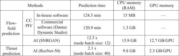
Finally, very fast predictions are possible with the developed deep-learning models, even when using high-resolution input particle images. The computation took only 12.5 s to predict 270 flow fields (approximately 600 times faster than the conventional CC-based PIV technique) and 2.1 s to predict the same amount of instantaneous rotor thrusts.
2. Data preparation
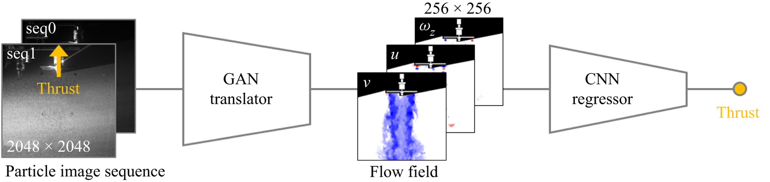
Figure 1 presents a schematic flow diagram of the AI architecture developed in this study. It consists of two parts: (i) particle-image-to-instantaneous-flow-field translation using a GAN model (Goodfellow et al. Reference Goodfellow, Pouget-Abadie, Mirza, Xu, Warde-Farley, Ozair, Courville and Bengio2014; Mirza & Osindero Reference Mirza and Osindero2014) and (ii) flow-field-to-thrust regression using a CNN model (He et al. Reference He, Zhang, Ren and Sun2016). The detailed structures of these models are presented in figures 3(a) (GAN) and 3(b) (CNN), respectively.
Schematic flow diagram of the proposed deep-learning architecture.

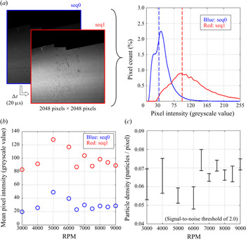
(a) A particle image pair example (left) and its pixel intensity (greyscale value) distribution (right). Vertical dashes represent mean of the distributions (blue, seq0; red, seq1), (b) mean pixel intensity and (c) particle density (seeding density, or particles per pixel), according to the rotor RPM.

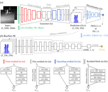
(a) Spectral-norm-based residual cGAN model (SNRGAN) for translating the input particle image sequence to the flow field. (b) CNN model for predicting the thrust from the flow field. At the bottom, legends for the residual blocks in (a,b) are presented. (c3s2, 3 × 3 convolution with stride 2; tc3s2, 3 × 3 transposed convolution (Zeiler et al. Reference Zeiler, Krishnan, Taylor and Fergus2010) with stride 2; IN, instance normalization of the layer (Ulyanov, Vedaldi & Lempitsky Reference Ulyanov, Vedaldi and Lempitsky2016); SN, spectral normalization of the weight; BN, batch normalization of the layer (Ioffe & Szegedy Reference Ioffe and Szegedy2015).)

For the data set-up, 1170 pairs of particle image sequences, flow fields calculated from them using a conventional PIV algorithm (CC) and thrust forces corresponding to each flow field were prepared experimentally using a drone rotor. A detailed description of the experimental set-up is provided in Lee et al. (Reference Lee, Chae, Woo, Jang and Kim2021). A particle image sequence consisted of two-channel images of 2048 × 2048 pixels, covering an area of 207 × 207 mm2, captured by a charge-coupled device camera with a time interval of 20 μs. An example of a pair of particle image sequences (seq0 and seq1) obtained at 8000 RPM is shown on the left side of figure 2(a). The image for seq1 is brighter (i.e. has higher pixel intensities) than that for seq0 because the camera exposure time for seq1 was set to be longer than that for seq0. Note that the rotor model and shadow cast by the model are masked in black at the top of the image; this area was excluded from the calculations when constructing the three graphs presented in figure 2.
The right side of figure 2(a) shows the pixel intensity distribution for the image sequences shown on the left side of the figure. The image pixel intensity for seq0 was concentrated from a greyscale value of 0 to approximately 110, with a mean value of 34; whereas that for seq1 was widely distributed, with a higher mean greyscale value of 97. Figure 2(b) shows the variation in the pixel intensity averaged over images taken at a given rotor speed. The mean pixel intensity of the particle image sequences used in this study varied with rotor speed in the range of 19–50 for seq0 and 83–128 for seq1, as shown in the figure. The particle images used differ not only in the pixel intensity distributions but also in the particle densities, depending on the rotor speed. The vertical bar in figure 2(c) indicates the particle density range with a signal-to-noise threshold of 2 in the images captured at a given rotor speed. As shown, the particle density in the images ranges from 0.048 particles/pixel to 0.08 particles/pixel, which corresponds to 12–20 particles in an interrogation window. The rotor speed was varied from 3000 to 9000 RPM (3000, 4000, 5000, 6000, 6500, 7000, 7500, 8000, 8500 and 9000; a total of ten RPM setpoints). The corresponding Reynolds numbers based on the rotor tip speed were 12 633, 16 844, 21 055, 25 266, 27 371, 29 477, 31 582, 33 688, 35 793 and 37 899, respectively. Consequently, particle images with diverse pixel intensity distributions, particle densities and RPM setpoints were included in the training data, allowing the development of a more robust deep-learning model. Note that consideration could also be given to introducing more variations in the data, such as employing noise in the input particle images, changing the particle size (currently 1 μm) or varying the laser light intensity (currently, 3.40 W cm−2).
Using the particle images described above, the flow field was calculated as a three-channel image consisting of instantaneous y-directional velocity v, x-directional velocity u and z-directional vorticity ωz (refer to figure 3a for the adopted coordinate system). A fast Fourier transform (FFT)-based CC algorithm was employed for the calculation using an in-house PIV software under the following conditions. An iterative CC analysis was conducted recursively from an initial interrogation size of 64 × 64 pixels to a final size of 16 × 16 pixels with a 50 % overlap, resulting in a corresponding spatial resolution of 1.08 % of the rotor diameter. The spurious vectors were detected with a local median filter that rejected vectors greater than three times the root mean square (r.m.s.) value of a 3 × 3 window. The outliers were replaced with linearly interpolated values from the neighbouring vectors. Image sharpening for the pixel-wise change in intensity was applied for image preprocessing, and polynomial subpixel interpolation was used to reduce errors and improve spatial accuracy. This method was applied in our previous studies (Chae et al. Reference Chae, Lee, Kim and Lee2019; Lee et al. Reference Lee, Chae, Woo, Jang and Kim2021) and has been proven to be accurate. The flow fields obtained using the above method were compared with those calculated using a commercial program (Dantec DynamicStudio) utilizing the same particle images for further validation. This comparison showed an MAE value of 0.0916 m s−1 (0.00350 when non-dimensionalized), root mean square error (RMSE) of 0.160 m s−1 (0.00597 when non-dimensionalized) and R 2 value of 96.185 %, confirming the reliability of the flow fields used in this study. The rotor thrust was measured simultaneously with the flow field by setting the force sampling rate equal to the PIV repetition rate. In this study, the particle image sequences, flow fields calculated from the images using CC and thrust forces corresponding to each flow field were treated as the ‘ground truth’ for the deep-learning models. Note that these ground-truth data are inherently imperfect and may contain errors.
Before training the models, the data were divided into training, validation and test datasets. Table 1 presents the detailed data configurations for the training, validation and test datasets, including the unit tensor size, quantity and occupied disk space. Each dataset contained the same amount of data for each RPM setpoint (e.g. the test data for the flow field included twenty-seven flow fields per RPM).
Data configurations for training, validation and test datasets, including unit tensor size, quantity and disk space occupied.

3. Deep-learning architecture
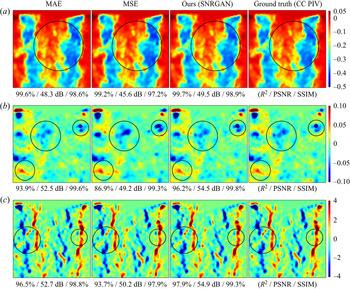
As depicted in figure 3(a), for instantaneous flow-field predictions (i.e. y-directional velocity v, x-directional velocity u and z-directional vorticity ωz), a GAN translator is adopted instead of a CNN-based encoder–decoder model with a regressive objective, which has been used in other AI studies. For CNN models using the mean absolute error or mean squared error as a cost function, the generated results tend to be blurry (Pathak et al. Reference Pathak, Krahenbuhl, Donahue, Darrell and Efros2016; Zhang et al. Reference Zhang, Isola and Efros2016; Isola et al. Reference Isola, Zhu, Zhou and Efros2017) because training is simply directed toward reducing the mean of the image difference. However, when a GAN is introduced, images with much better quality (i.e. higher accuracy) can be generated because the discriminator imposes a penalty on patches assessed to be different from their real representations, such as blurred areas. (Detailed comparison results can be found in Appendix C.) Moreover, in our GAN model, the computational cost of the discriminator is much lower than that of the generator (~1 %), resulting in an efficient accuracy improvement. High-quality flow generation also helps improve the performance of the thrust prediction model because it takes the predicted flow field as an input during evaluation.
As presented in figure 3(a), the developed GAN model is composed of two trainable functions, namely, the flow-field generator and discriminator (denoted by G and D, respectively). First, the generator accepts an experimentally observed particle image sequence (denoted by c) and translates it into an instantaneous flow field (a three-channel flow-field image; denoted by G(c)) through deep convolution layers. To avoid damaging the particle information, a 2048 × 2048-pixel high-resolution input particle image was used without any preprocessing (e.g. interpolation to low resolutions). Moreover, to stack many layers in a stable manner (i.e. for a secure gradient propagation), a residual connection was utilized (Gross & Wilber Reference Gross and Wilber2016; He et al. Reference He, Zhang, Ren and Sun2016; Wang et al. Reference Wang, Liu, Zhu, Tao, Kautz and Catanzaro2018) throughout the generator. Furthermore, to stabilize adversarial training, which is known to be difficult because the objectives of the two components head in opposite directions, spectral normalization (Horn & Johnson Reference Horn and Johnson2012) was applied to every convolutional weight in the generator (Zhang et al. Reference Zhang, Goodfellow, Metaxas and Odena2019) and discriminator (Miyato et al. Reference Miyato, Kataoka, Koyama and Yoshida2018). The detailed structures of the residual blocks are presented at the bottom of figure 3.
Second, the discriminator is trained to classify half the data (ground truth, i.e. FFT-based cross-correlated flow field; denoted by t) as real data and the other half (G(c)) as fake data on patches (Isola et al. Reference Isola, Zhu, Zhou and Efros2017) through five convolution layers. This is achieved by minimizing the given loss function  ${{\mathcal{L}}_D}$ (Mao et al. Reference Mao, Li, Xie, Lau, Wang and Paul Smolley2017) (
 $\mathrm{\mathbb{E}}$, expectation; p, probability distribution):
 \begin{equation}{{\mathcal{L}}_D} = {\textstyle{1 \over 2}}{\mathrm{\mathbb{E}}_{t,c\sim {p_{data}}(t,c)}}[{(D(t|c) - 1)^2}] + {\textstyle{1 \over 2}}{\mathrm{\mathbb{E}}_{c\sim {p_{data}}(c)}}[{(D(G(c)|c))^2}].\end{equation}
Thus, the discriminator strives to make  $D(t|c)$ near 1 and
 $D(G(c)|c)$ near 0. In contrast, the generator loss function
 ${{\mathcal{L}}_G}$ is given by
 \begin{equation}{{\mathcal{L}}_G} = \frac{1}{2}{\mathrm{\mathbb{E}}_{c\sim {p_{data}}(c)}}[{(D(G(c)|c) - 1)^2}] + \lambda \sum\limits_{l = 1}^L {\frac{1}{{{N_l}}}[{\parallel} {D^{(l)}}(G(c)|c) - {D^{(l)}}(t|c){\parallel _1}]} ,\end{equation}
where the feature-matching loss (Johnson, Alahi & Fei-Fei Reference Johnson, Alahi and Fei-Fei2016) is additionally introduced to match the intermediate representations recognized by D (λ = 100; the number of D inner layers L = 4; Nl is the number of elements in the lth layer). The feature-matching loss stabilizes GAN learning and has a good effect on style transfer (Johnson et al. Reference Johnson, Alahi and Fei-Fei2016). Furthermore, without spectral normalization or the feature-matching term, or a small λ, an equilibrium between G and D could not be reached. By minimizing (3.2), the generator tries to make  $D(G(c)|c)$ near 1 and
 ${D^{(l)}}(G(c)|c)$ approach
 ${D^{(l)}}(t|c)$, creating more realistic sharp flow fields as the training proceeds. Therefore, when adversarial learning is stably and sufficiently progressed, and if G and D have sufficient capacity, the probability distribution of the prediction approaches that of the ground truth (pG (c) → pt). Finally, an equilibrium is reached, as shown at the top of figure 4(a) (at near 500 epochs; at this point, the discriminator cannot differentiate between G(c) and t, that is,
 $D(G(c)|c) = D(t|c) = 0.5$. Both values cannot improve as pG (c) = pt (Goodfellow et al. Reference Goodfellow, Pouget-Abadie, Mirza, Xu, Warde-Farley, Ozair, Courville and Bengio2014)). Thus, using our spectral-norm-based residual conditional GAN architecture, a very stable high-resolution image-to-image translation was possible with a superior generation quality. The developed GAN translator can also be applied to other domain sizes by simply adding or removing the front or upscaling residuals and adjusting the number of intermediate residual blocks, as shown in figure 3(a). More details about the model and loss function can be found in Appendix A (generator), Appendix B (discriminator) or the referenced articles. They are omitted here for conciseness.
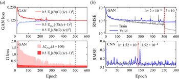
(a) Profile of the GAN train loss (top) and generator loss (bottom). (b) RMSE profile of the GAN translator (top) and CNN regressor (bottom) for the training (grey) and validation (blue) datasets.

Third, the thrust-predicting CNN model was trained as shown in figure 3(b), and its unit structure is presented at the bottom right corner of the figure. It is a well-known ResNet-50 feature recognizer (Gross & Wilber Reference Gross and Wilber2016; He et al. Reference He, Zhang, Ren and Sun2016). The extracted features are regressed into a scalar value, the instantaneous thrust, by minimizing the following MSE  ${{\mathcal{L}}_F}$ (F, ResNet-50, T, experimentally measured thrust using a load cell):
 \begin{equation}{{\mathcal{L}}_F} = {(F(t) - T)^2}.\end{equation}
Note that, although ResNet is not the most recent model in image recognition, it still attains very good performance (Kolesnikov et al. Reference Kolesnikov, Beyer, Zhai, Puigcerver, Yung, Gelly and Houlsby2019) and is based on a simple and intuitive architecture.
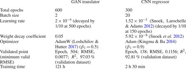
In figure 4(a), the profiles of the GAN train and generator losses are shown in the top and bottom parts, respectively. The figure indicates that the model was successfully trained and reached an equilibrium with a near-zero feature-matching loss (0.068 × 10⁻² at epoch 504). Figure 4(b) presents the RMSE profiles of the two AI models (top: GAN translator, bottom: CNN regressor) for the training (grey) and validation (blue) datasets. The RMSE and R 2 accuracies for the flow-field prediction were calculated after masking (excluding) the rotor area in this study (see the black masked area presented in figure 1, including the rotor). The red vertical line in each graph indicates the validation epoch number, at which the final performance of the model was evaluated using the test dataset.
Both models were trained from scratch with PyTorch using dual TITAN RTX GPUs, and the details of the training hyperparameters are summarized in table 2. The training data were pre-augmented by applying a horizontal flip (thus, 700 × 2 pairs) to both models. For the GAN translator, the number of D training steps was four, whereas that of G training steps was one for each batch iteration (better results were obtained when the D train step was larger than the G train step, as reported in Arjovsky, Chintala & Bottou Reference Arjovsky, Chintala and Bottou2017). Moreover, the AdamW optimizer (Loshchilov & Hutter Reference Loshchilov and Hutter2017) showed a better performance with our GAN model than that of Adam optimizer (Kingma & Ba Reference Kingma and Ba2014). (See Appendix D for more details on the computational set-ups.)
Information regarding the data and training of the two developed AI models.

4. Results and discussion
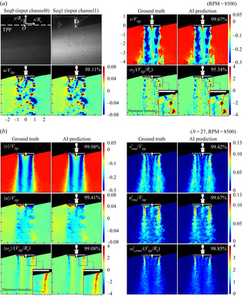
In this section, the performance of the developed AI model is demonstrated using the test dataset (namely, the data not used in any training or validation process). In figure 5(a), the particle image sequence inputted to the GAN translator (top left two images) and predicted instantaneous flow fields are shown (top right, v; left bottom, u; and right bottom, ωz). In each field, the ground truth and prediction are displayed on the left and right sides, respectively, with the R 2 accuracy written at the top-right corner. One randomly selected datum out of a total of 270 test data is shown in the figure after the non-dimensionalization of the values and axes (Vtip, rotor tip velocity; Rr, rotor radius (38 mm)). In the first particle image, the employed Cartesian coordinates are marked with the tip path plane (TPP).
(a) Predicted instantaneous flow field using the developed GAN translator. (b) Statistical turbulent flow field obtained from the 27 predicted instantaneous flow fields at 8500 RPM.

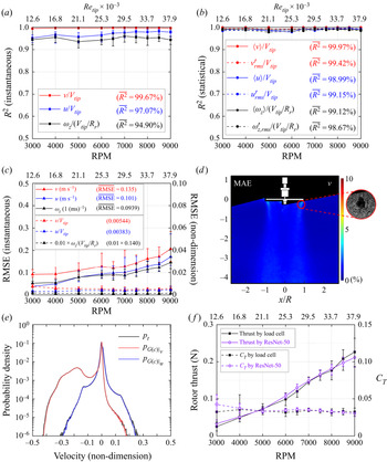
As shown in the figure, the prediction is so accurate that the ground truth (t) and AI generation (G(c)) are almost indistinguishable, as was the goal of the GAN. In figure 6(a), the R 2 accuracy of the instantaneous flow-field prediction with respect to RPM (bottom x-axis) and Reynolds number based on the rotor tip speed ( $R{e_{tip}}$; top x-axis) is plotted (each scatter point denotes the mean of the accuracy for the 27 test samples). (
 $R{e_{tip}} = {V_{tip}}c/\nu $, where c and ν denote the chord length of the rotor blade (0.016 m) and kinematic viscosity of air, respectively.) The RPM-wise (or
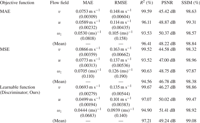
 $R{e_{tip}}$-wise) mean accuracy was 99.67 % for v, 97.07 % for u and 94.90 % for ωz (their average is 97.21 %). This result demonstrated the capability of the developed GAN translator. Note that the accuracies and errors in this study were calculated after excluding the rotor area, as mentioned earlier.
Prediction accuracies for (a) the instantaneous flow field and (b) statistical turbulent flow field, versus the rotor RPM (bottom x-axis) and Reynolds number based on the rotor tip speed (Retip; top x-axis). Note that non-dimensionalization does not affect the accuracy. (c) RPM-wise (or Retip-wise) RMSE (solid lines; left y-axis) and non-dimensionalized RMSE (dashed lines; right y-axis) for the instantaneous flow field. (d) MAE map for the streamwise velocity v on a y/R–x/R plane. It was normalized with respect to the v range. (e) Probability density of the instantaneous velocity (black, ground truth; red, predicted v; and blue, predicted u; c and t, entire test data). ( f) Results of the instantaneous rotor thrust prediction using the CNN regressor (black, ground truth measured by the load cell; violet, AI prediction). Solid and dashed lines denote rotor thrust (left y-axis) and thrust coefficient CT (right y-axis), respectively, according to the rotor RPM (bottom x-axis) and Retip (top x-axis).

In figure 5(b), using the predicted instantaneous flow fields, a statistical turbulent flow field is constructed (top left,  $\langle v\rangle /{V_{tip}}$; top right,
 ${v^{\prime}_{rms}}/{V_{tip}}$; middle left,
 $\langle v\rangle /{V_{tip}}$; middle right,
 ${u^{\prime}_{rms}}/{V_{tip}}$; bottom left,
 $\langle {\omega _z}\rangle /({V_{tip}}/R_{r})$; and bottom right,
 ${\omega ^{\prime}_{z,rms}}/({V_{tip}}/R_{r})$;
 $\langle \,\rangle $: time average; apostrophe r.m.s., r.m.s., velocity fluctuation; number of samples, 27; RPM, 8500). Figure 6(b) depicts the R 2 accuracy of the mean and r.m.s. flow fields for all RPMs (for all
 $R{e_{tip}}$s). Because the instantaneous flow-field prediction was accurate, the mean and r.m.s. flow fields also showed a high accuracy of approximately 99 %, even in a region with high turbulence (i.e. a large r.m.s. region). Note that the r.m.s. velocity fluctuations were more prominent in the x-direction than they were in the y-direction (compare the contours of
 ${u^{\prime}_{rms}}/{V_{tip}}$ with
 ${v^{\prime}_{rms}}/{V_{tip}}$) along the trajectory of the rotor tip vortices close to the TPP. This indicates that the tip vortices ‘wander’ mainly in the direction normal to their trajectory. The mean trajectory of the tip vortices is called the slipstream boundary and is shown as a black dashed curve in the enlarged inset of the
 $\langle {\omega _z}\rangle /({V_{tip}}/R_{r})$ contour. To demonstrate the wandering motion of the tip vortices, the slipstream boundary was overlapped on the normalized instantaneous vorticity contour (see the enlarged inset in the lower right panel of figure 5a). As shown in the figure, the rotor tip vortices convected downstream, deviating from side to side with respect to the slipstream boundary. It has been suggested that vortex wandering is induced by inflow unsteadiness, shear layer turbulence and cooperative instabilities (Mula et al. Reference Mula, Stephenson, Tinney and Sirohi2013). Considering that wake geometry plays an essential role when assessing the aerodynamic performance, such as rotor efficiency and blade loads (Landgrebe Reference Landgrebe1972; Leishman, Baker & Coyne Reference Leishman, Baker and Coyne1996; Leishman Reference Leishman1998; Lee et al. Reference Lee, Chae, Woo, Jang and Kim2021), vortex wandering hinders the accurate prediction of drone performance because it makes it difficult to predict the rotor wake boundary. Thus, vortex wandering requires further investigation. The accurate prediction method presented in this study will pave the way for further detailed studies on the underlying mechanism of vortex wandering.
To assess the quality of the flow-field prediction, the RMSE of the instantaneous flow-field prediction and MAE map for the y-directional (streamwise) velocity v are presented in figures 6(c) and 6(d), respectively (the error map was normalized with respect to the v range). In figure 6(c), the RMSE and its non-dimensionalized value are shown as solid and dashed lines on the left and right y-axes, respectively, according to the RPM (bottom x-axis) and  $R{e_{tip}}$ (top x-axis). As shown in the figure, the RPM-wise (or
 $R{e_{tip}}$-wise) mean RMSE is 0.135 m s−1 for v (0.00544 for v/Vtip), 0.101 m s−1 for u (0.00383 for u/Vtip) and 0.0939 ms for ωz (0.140 for ωz/(Vtip/R)). As the RPM increased, the error also increased (solid lines), which is a mathematically natural behaviour because the magnitudes of v, u and ωz increase with the RPM. As shown in the error map presented in figure 6(d), the error was nearly zero over the entire domain, except for the area along the trajectory of the tip vortices near the rotor tip (red-circled area; the maximum error was 2.91 %). The relatively large MAE near the rotor tip is due to a locally low particle density. As shown in the enlarged inset of figure 6(d), there is a region where few particles are observed. This region is known to be formed as the centrifugal force induced by the rotor tip vortex causes the seeding particles to move radially outward from the vortex core (Leishman Reference Leishman1998). Because there are few particles in this black void area, CC-based PIV predicts the flow using a series of image processing techniques, such as subpixel interpolation. Because the AI learned by looking at the results obtained in this manner, the accuracy in that area was inevitably lower than that in other areas that directly matched the flow field from the particle information. In addition, because the ground truth itself included errors due to interpolation, it was natural to observe larger errors in AI prediction in that area. However, even if the error was larger, it was less than 3 %, which is acceptable. Finally, in addition to the RMSE and error map, the MAE, peak signal-to-noise ratio (PSNR) and structural similarity (SSIM) (Wang et al. Reference Wang, Bovik, Sheikh and Simoncelli2004) were calculated. The RPM-wise mean MAE values were 0.0693 m s−1 for v, 0.0499 m s−1 for u and 0.0444 (ms)‒1 for ωz (non-dimensionalized MAE values were 0.00279 for v, 0.00194 for u and 0.0683 for ωz). The PSNR values were 46.27 dB for v, 50.02 dB for u and 51.41 dB for ωz (their average was 49.24 dB). The values of SSIM were 98.86 % for v, 99.47 % for u and 98.92 % for ωz (an average of 99.08 %). (See table 3 in Appendix C for the tabulated data.)
In figure 6(e), the probability distributions of the instantaneous velocity for prediction (pG (c)) and ground-truth (pt) values are plotted on a probability density–velocity plane (black, ground truth; red, predicted v; and blue, predicted u; c and t, entire test data; rotor area excluded). As shown in the figure, the distributions of the predictions faithfully follow those of the ground truths, even for the test data, underlining the good generalization ability of the model with minimal overfitting.
From the predicted instantaneous flow field (G(c)), instantaneous rotor thrust was predicted using the proposed CNN regressor, and the results are presented in figure 6( f). The black and violet lines denote the measured and predicted thrusts, respectively, with respect to the rotor RPM (bottom x-axis) and  $R{e_{tip}}$ (top x-axis). The solid and dashed lines represent the rotor thrust (left y-axis) and thrust coefficient CT (right y-axis), respectively. The value of CT was calculated as
 $T/(\rho AV_{tip}^2)$, where T, ρ and A denote the rotor thrust, density of air and rotor disk area (
 ${\rm \pi} R^2_r$), respectively. The R 2 accuracy is 94.57 %, suggesting that instantaneous rotor thrust can be accurately predicted using deep learning from only the flow-field information without any additional measuring equipment. Note that when the rotor thrust is predicted with additional experimental data for RPM setpoints of 3500, 4500 and 5500, accuracy is 92.71 %, 96.01 % and 97.29 %, respectively.
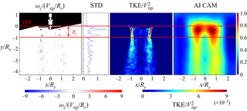
In figure 7, from left to right, the input vorticity field, its y-directional standard deviation  $({\sigma _y}(|{{\omega_z}/({V_{tip}}/R_{r})} |))$, which reveals the relative strength of vorticity according to y, a contour of turbulent kinetic energy (TKE; normalized with respect to
 $V_{tip}^2$) and a class activation map (CAM) (Zhou et al. Reference Zhou, Khosla, Lapedriza, Oliva and Torralba2016) are presented. A TKE contour demonstrates a long growth of TKE along the trajectory of the rotor tip vortices, called the slipstream boundary, where it appears high in the area from the TPP down to one rotor radius (Rr) and gradually weakens downstream. This result indicates that when the tip vortices formed by the rotor rotation are periodically convected downstream, they maintain a distinct shape downstream to y/R r = −1 but are mixed and dissipated later. This result can also be confirmed with the instantaneous vorticity contours. In the region where the tip vortices remain distinct (from TPP down to 1Rr), the streamwise velocity is accelerated because the wake-induced velocity exists within the slipstream boundary. Subsequently, the wake region begins to decelerate as the wake spreads widely and decays owing to the viscous effect.
From left to right: input instantaneous vorticity, y-directional standard deviation of absolute vorticity, turbulent kinetic energy  $(\textrm{TKE/}V_{tip}^2)$ and CAM at 7500 RPM.

As shown in figure 7, CAM is highly activated within the 1Rr section under TPP (inside the area bounded by two horizontal red lines). CAM was used to investigate where the CNN model was looking when making predictions. Thus, the AI model examined this area and predicted the thrust. In this 1Rr region, as shown in the figure, energy is continuously provided by the rotor rotation and dominant wake structures are maintained. After this region (toward −y), the energy supplied by the rotor is consumed and the momentum is dissipated (wake structures are demolished). The thrust is proportional to the energy supplied by the rotor (according to momentum theory). The AI model examined the area where the energy was provided and made predictions, thus the model succeeded in capturing the underlying physics by itself and was trained properly. The only information provided to the model was the input instantaneous flow field and corresponding thrust value.
The computational factors for time and memory consumption are presented in Appendix D along with a comparison against the conventional CC-based PIV method. Specifically, the prediction took only 12.5 s for the GAN translator (nearly 600 times faster than the CC PIV) and 2.1 s for the CNN regressor when using 270 test datasets. The two AI models presented in this study (GAN translator and CNN regressor) can be utilized separately; therefore, the developed CNN regressor can be applied to a flow field obtained from an existing PIV technique, such as CC and OF, to predict the instantaneous rotor thrust.
5. Conclusions
In this study, a novel deep-learning architecture was proposed to predict the instantaneous flow field and thrust under a single drone rotor from PIV-observed particle images. A real-world complex turbulent flow induced by the high-speed rotation of a rotor (up to 9000 RPM) was examined. Two different deep-learning models were presented, and the main results of this study can be summarized as follows:
(i) For a highly accurate prediction of the instantaneous flow field from high-resolution particle images (2048 × 2048 pixels), a GAN framework was introduced for the first time instead of a conventional CNN-based encoder–decoder model with a regressive objective. The developed model was a spectral-norm-based residual conditional GAN (SNRGAN), which can conduct highly stable adversarial training and yield high-accuracy predictions. Training hyperparameters optimized for the model were also presented.
(ii) The mean accuracy for the instantaneous flow-field prediction was 97.21 % (R 2), 49.24 dB (PSNR) and 99.08 % (SSIM). The prediction was accurate for all RPM ranges (i.e. 3000–9000). Moreover, the probability distributions of the prediction and ground-truth values were well matched, demonstrating the good generalization ability of the developed GAN model with minimal overfitting.
(iii) For the first time, instantaneous rotor thrust was predicted using a deep CNN model (ResNet-50) from an instantaneous flow field. For the regression task, the last classifier was replaced with a linear regressor, and the MSE cost function was employed. The prediction accuracy was 94.57 %, which highlights the potential of AI methods in drone thrust prediction. Moreover, where the model examined and made predictions, as well as whether the training proceeded properly from a physical standpoint, were discussed. The results confirmed that the trained AI model predicted the thrust by spontaneously recognizing the part that received kinetic energy from the rotor.
(iv) The developed deep-learning models significantly improved the computational speed. The flow-field calculation took only 12.5 s for 270 test datasets, whereas it took 120–125 min using the conventional CC-based PIV technique (nearly 600 times slower compared with the proposed method). For thrust prediction, it only took 2.1 s for the same amount of data. Consequently, with our deep-learning architecture, a high-accuracy and high-speed solution can be achieved even with real-world complex turbulent flow data.
Funding
This research was supported by the Basic Science Research Program of the National Research Foundation (NRF) of Korea, funded by the Ministry of Science and ICT (grant no. NRF-2019R1A2C2089114).
Declaration of interests
The authors report no conflict of interest.
Appendix A. Architecture of the GAN generator
Our GAN generator has a spectral-norm-based residual convolutional encoder–decoder structure, which consists of four stages: a stem stage, front residuals, intermediate residuals and back residuals, as presented in figure 3. Here, c7s1-k denotes a 7 × 7 convolution with k filters and a stride of 1. Rd-k denotes a downscaling residual block consisting of (c3s2-k, IN, ReLU, c3s1-k, IN) and (c1s2-k, IN), where IN and ReLU represent instance normalization and rectified linear units (Nair & Hinton Reference Nair and Hinton2010), respectively. Note that, in this paragraph, the former and latter parentheses indicate the main operations and residual shortcut operations, respectively. Ru-k denotes an upscaling residual block composed of (tc3s2-k, IN, ReLU, c3s1-k, IN) and (tc1s2-k, IN), where tc represents the transposed convolution (output padding = 1). R-k denotes a normal residual block consisting of (c3s1-k, IN, ReLU, c3s1-k, IN) with an identity residual summation ((c1s1-k, IN) if the number of channels changes). In every residual block, the padding was 1 for the main convolutions and 0 for the shortcut convolution. Spectral normalization was applied to all convolutional weights. All biases were off to reduce overfitting. The architecture of the generator is as follows.
(i) Stem stage: c7s1-32 (padding = 3), IN, ReLU.
(ii) Front residuals: Rd-64, Rd-128, Rd-256, Rd-512, Rd-1024.
(iii) Intermediate residuals: R-1024 × 15.
(iv) Back residuals: Ru-512, Ru-256, R-128, R-64, R-3*.
(*The last R-3 block is (c3s1-3, IN, ReLU, c3s1-3) and (c1s1-3), with the last tanh activation.)
Appendix B. Architecture of the GAN discriminator
Our GAN discriminator is a patchGAN-style (Isola et al. Reference Isola, Zhu, Zhou and Efros2017) spectral-norm-based encoder. Here, c4s2-k-L denotes a 4 × 4 convolution with k filters and a stride of 2 (padding = 1), followed by a leaky ReLU (Maas, Hannun & Ng Reference Maas, Hannun and Ng2013) (negative slope = 0.2 (Radford, Metz & Chintala Reference Radford, Metz and Chintala2015)). Spectral normalization was applied to all convolutional weights, and all layer normalizations were cancelled accordingly (Miyato et al. Reference Miyato, Kataoka, Koyama and Yoshida2018). All biases were off. The architecture of the discriminator is as follows.
(i) Channel concatenation between
 $G(c)$ (tensor size, (3, 256, 256)) and c after average pooling (tensor size, (2, 256, 256)): $G(c)|c$ (tensor size, (5, 256, 256)).
(ii) c4s2-64-L, c4s2-128-L, c4s2-256-L, c4s1-512-L, c4s1-1.


Appendix C. Performance comparison based on objective function of flow-field generator
Tests were conducted by changing the objective function of the flow-field generator to determine the effectiveness of the employed GAN architecture compared with a normal CNN-based encoder–decoder structure with a regressive objective (that is, training without the discriminator having the structure of the flow-field generator presented in Appendix A fixed). Two conventional regressive objective functions, namely, MAE and MSE, were tested, whose results are presented in table 3. A total of 270 test datasets were used as input, and the MAE, RMSE, R 2, PSNR and SSIM metrics were assessed. As previously mentioned, our SNRGAN model attained the best performance in terms of these five metrics. Because all three models shared the same generator structure, the computational costs incurred for the prediction were the same (the discriminator of the GAN did not participate in the prediction).
Performance comparison based on objective function of flow-field generator using 270 test datasets. The structure of the generator was fixed to that described in Appendix A. Numbers in parentheses in the third and fourth columns were non-dimensionalized errors.

For a visual comparison of the generation quality, figure 8 presents, from left to right, the generation results obtained from the objective functions of MAE, MSE, discriminator (SNRGAN) and ground truth, respectively. Non-dimensionalized v, u and ωz maps are shown from top to bottom, respectively. The RPM is 3000, and the domain of each figure corresponds to the square area from −1 to 1 on the x/R r-axis and −2 to 0 on the y/R r-axis in figure 5(a). The R 2, PSNR and SSIM quality assessment metrics measured in the given square area are provided sequentially below each flow-field prediction map. Because of the deep residual layers, the MAE and MSE objectives demonstrate competitive results in terms of R 2, PSNR and SSIM. However, areas with blurring or missing details are often observed (circled areas), which reveals the innate limitation of the regressive cost functions. On the other hand, our GAN model obtains high-quality predictions that are clear and sharp, with abundant details for the flow field. The metrics for SNRGAN were the best as well. Note that, as presented in the results for the MAE and MSE objectives in figure 8, the R 2, PSNR and SSIM assessment metrics do not seem to fully reflect the true perceptual similarity (the calculated metrics are still good despite the missing sharp details), which has been actively investigated in the field of computer vision (Heusel et al. Reference Heusel, Ramsauer, Unterthiner, Nessler and Hochreiter2017; Ledig et al. Reference Ledig, Theis, Huszãr, Caballero, Cunningham, Acosta, Aitken, Tejani, Totz and Wang2017; Blau & Michaeli Reference Blau and Michaeli2018; Zhang et al. Reference Zhang, Isola, Efros, Shechtman and Wang2018; Gu et al. Reference Gu, Cai, Chen, Ye, Ren and Dong2020).
Visual comparison of flow-field prediction results based on objective functions (MAE, MSE, discriminator and ground truth from left to right, respectively), with a fixed generator structure. The non-dimensionalized v, u and ωz maps are shown from (a) to (c), respectively, at 3000 RPM.

Appendix D. Computational cost and comparison with conventional CC-based PIV method
The computational cost was measured using conventional CC-based PIV techniques (in-house software and commercial software (Dantec DynamicStudio)) and deep-learning models (GAN translator and CNN regressor); the results are presented in table 4. The tests were conducted using 270 test datasets (see table 1 for the detailed data configuration). CC-based PIV techniques were performed on an Intel® i5-7500 CPU (3.4 GHz) desktop computer, including the extraction of velocities, data smoothing and vorticity calculations. The two deep-learning models were tested on an AMD EPYC™ 7282 CPU (2.8 GHz) computer aided by four Nvidia RTX A5000 GPUs using PyTorch. Each of these two sets of computational specifications represents a computer environment commonly used in conventional PIV and deep learning. In the case of AI GPU computing, time and memory consumption were measured using GPU distributed data parallelism (DDP). In addition, to accelerate data loading, two subprocesses were utilized per worker process, with compute unified device architecture (CUDA)-pinned memory prefetching and GPU asynchronous copy. Note that this set-up was used for training as well. As shown in table 4, the AI computation was much faster (approximately 600 times) than the CC-based PIV techniques because of the DDP-based general-purpose computing on graphics processing units (GPGPU) computing, which is well optimized for a neural network. Although AIs require a larger memory, it is reasonable from the point of view of an actual user. In the case of thrust prediction, the prediction time was only 2.1 s, as presented in the table, underlining the high potential of deep learning in real-time thrust prediction applications. One could also consider employing a quantization technique for AI models to decrease the computational cost. Memory usage is known to decrease by a factor of four (float32-to-int8), with a 2–4 times faster computational speed, when typical float32 tensors are replaced by 8-bit integer-type tensors (lower bitwidths) (PyTorch 2021).
Comparison of computation factors using 270 test datasets.

Appendix E. Test on a different rotor model and toward generalizations
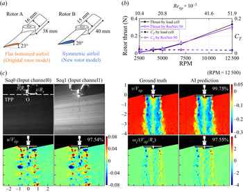
To demonstrate the generalization ability of the AI model for different rotor geometries, the proposed architecture was additionally tested using a different configuration of the drone rotor operating at five Reynolds numbers. Figure 9(a) presents two rotor models – the left one is the rotor used routinely in this study (having a flat-bottomed airfoil; denoted by rotor A) and the right one is the new rotor introduced to test the AI models (having a symmetric airfoil; denoted by rotor B). Both rotor models have untwisted rectangular blades, and their rotor radii, blade pitch angles and chord lengths are reported in the figures. RPM setpoints for the new rotor were 2500, 4000, 5000, 7000 and 12 500 (corresponding  $R{e_{tip}}$s were 10 389, 16 622, 20 778, 29 089 and 51 944, respectively).
(a) Rotor models (left, rotor A – the original rotor model; right, rotor B – a new rotor model). (b) Thrust prediction result for rotor B using the trained CNN regressor. (c) Instantaneous flow-field prediction result for rotor B using the trained GAN translator.

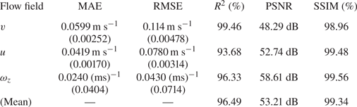
Using one hundred rotor B data (i.e. particle image sequences taken from rotor B, flow fields calculated from them using CC and thrust forces corresponding to each flow field), the developed GAN translator and CNN regressor were tested. Subsequently, R 2 accuracies of 96.49% and 96.79% were obtained for the flow-field prediction and thrust prediction, respectively. In figure 9(c), the particle image sequence inputted to the GAN translator (top left two images) and predicted instantaneous flow fields with their ground truths are shown (top right: v, bottom left: u and bottom right: ωz) after non-dimensionalization. As expected, the differences between the prediction results and ground truths were minimal. The prediction metrics of MAE, RMSE, R 2, PSNR and SSIM are listed in table 5. Figure 9(b) presents the thrust prediction result, which showed good accuracy even with a smaller or larger Reynolds number than that used for training.
Errors and accuracies of flow-field prediction under a new rotor (rotor B in figure 9a). Numbers in parentheses are non-dimensionalized errors.

Note that the predictions for rotor B were safely conducted, as its data had a probability distribution similar to that of the existing rotor. (The geometric type of blade, rotor radius, blade pitch angle and chord length of rotor B were not significantly different from those of rotor A.) However, if a rotor with a radius of 150 mm is used (nearly 4 times bigger than rotor A), machine learning techniques, such as fine tuning or transfer learning, might be required to effectively broaden visual field of AI models or to quickly adapt them to new targets (TensorFlow 2021). Such as example in computer vision is applying the prior knowledge obtained from learning to recognize cars to the task of recognizing buses. Specifically, it entails taking an AI model that has already been trained on some data and training it a little further using new data (and possibly with the original data). With this approach, it is possible to effectively broaden and deepen the knowledge of AI, and move toward generalization.