1. Introduction
The symmetric instability (SI) is an instability of baroclinic zonal flows where perturbations contain no longitudinal variation, and are thus two-dimensional. The baroclinic zonal flow model (Eady Reference Eady1949), a fundamental geophysical flow problem that is discussed by Pedlosky (Reference Pedlosky1987), takes the form of a sheared flow
 $u(z)$
that balances a density field of the form
 ${\it\rho}(y,z)$
in a rotating frame. Here,
 $N^{2}=-(g/{\it\rho}_{0})\partial {\it\rho}/\partial x_{3}$
is the buoyancy frequency,
 $f$
is the Coriolis parameter and
 $S^{2}=(\Vert \partial \boldsymbol{u}_{h}/\partial x_{3}\Vert )^{2}$
is the squared vertical shear of horizontal velocity components. Also,
 $x$
,
 $y$
,
 $z$
or
 $x_{1}$
,
 $x_{2}$
,
 $x_{3}$
are used to denote streamwise, spanwise and vertical coordinates. The symmetric instability dominates the instability of the Eady flow when the Richardson number
 $(Ri=N^{2}/S^{2})$
is between
 $0.25$
and
 $0.95$
, while baroclinic and Kelvin–Helmholtz (K–H) instabilities dominate at higher and lower
 $Ri$
respectively, as shown by Stone (Reference Stone1966). In a more general case that includes relative vorticity
 ${\it\omega}_{i}$
due to horizontal shear (
 $\partial u/\partial y$
), instability is manifested when the potential vorticity (PV,
 $q=-{\it\rho}_{0}^{-1}({\it\omega}_{i}+f{\it\delta}_{i3})\partial {\it\rho}/\partial x_{i}$
) is of opposite sign to the Coriolis parameter in stably stratified regions, as noted in Hoskins (Reference Hoskins1974). These more general flows are susceptible to inertial/centrifugal and symmetric instabilities which act on the absolute vertical vorticity opposing planetary rotation and vertical shear respectively. In general, balanced baroclinic zonal flows have PV given by
 $q=-fS^{2}+({\it\omega}_{3}+f)N^{2}$
(Thomas et al.
Reference Thomas, Taylor, Ferrari and Joyce2013). Therefore, since
 $S^{2}=M^{4}/f^{2}$
for a balanced zonal flow with
 $M^{2}=-(g/{\it\rho}_{0})\partial {\it\rho}/\partial x_{2}$
, the PV may take the opposite sign of
 $f$
for a sufficiently strong front with large cross-front buoyancy gradient,
 $M^{2}$
.
An exceptionally sharp (1 km) front near the beginning of the Kuroshio extension was investigated by D’Asaro et al. (Reference D’Asaro, Lee, Rainville, Harcourt and Thomas2011). Shipboard measurements, a Lagrangian float and a towed profiling vehicle allowed for measurements of the turbulence intensity (inferred from vertical motions of the float), temperature, salinity, pressure and velocity profiles. The front is less than 1 km wide and approximately 20 m deep, and contains vertical motion resulting from upper-ocean turbulence. Dissipation at the front is estimated to be 10–20 times stronger than outside the front, but surface winds and cooling are too weak to explain the observed turbulence. The PV was found to take the opposite sign of
 $f$
for
 $0.2$
days while the vessel passed through the front, strongly suggesting symmetric instability as the relevant mechanism. These results imply that in some regions of the upper ocean, lateral density gradients and symmetric instability may be more important than atmospheric forcing in setting the turbulence intensity.
The evolution of a symmetrically unstable density frontal zone is examined using linear stability theory and two-dimensional nonlinear numerical simulations in Taylor & Ferrari (Reference Taylor and Ferrari2009). The a priori assumption of symmetric instability (no along-front or
 $x_{1}$
variation in figure 1), also adopted in previous numerical studies of the problem by Thorpe & Rotunno (Reference Thorpe and Rotunno1989) and Griffiths (Reference Griffiths2003a
,Reference Griffiths
b
), allowed Taylor & Ferrari (Reference Taylor and Ferrari2009) to employ the two-dimensional
 $(x_{2},x_{3})$
approximation for the flow. Linear stability analysis demonstrated that for large
 $|N/f|$
, viscous effects on the slopes of the symmetric currents are negligible and that
 $Ri<0.25$
is satisfied locally before the symmetric currents become fully nonlinear. Once the instability reaches finite amplitude, a secondary K–H instability forms. Following the secondary instability, small-scale turbulence entrains positive PV into the mixed layer from the thermocline, resulting in a rapid equilibration of the flow as the PV approaches zero throughout the mixed layer.
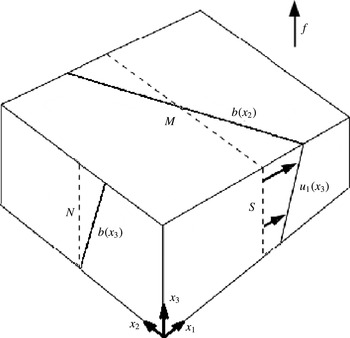
Schematic showing a stratified vertically sheared flow,
 $u_{1}(x_{3})$
, in thermal wind balance representing a small subsection of a stably stratified frontal zone. Spatial gradients in velocity and buoyancy are shown along with their respective time scales. Here,
 $M^{2}=\partial b/\partial x_{2}$
,
 $N^{2}=\partial b/\partial x_{3}$
and
 $S=\partial u_{1}/\partial x_{3}$
. The along-front direction is
 $x_{1}$
and the lateral (spanwise) direction is
 $x_{2}$
.

Instabilities in a baroclinic zonal flow are explored in Molemaker, McWilliams & Capet (Reference Molemaker, McWilliams and Capet2010) using quasigeostrophic and Boussinesq nonlinear simulations. This study explores the emergence of a forward energy cascade in a flow with
 $Ro=|S/f|<1$
but not
 $Ro\ll 1$
, with
 $Ri=N^{2}/S^{2}>1$
. The domain size is too small to observe the baroclinic instability, while
 $Ri$
is too large for symmetric instability. Turbulence in the Boussinesq case emerges via the generation of sharp fronts (locally
 $Ri<1$
and
 $Ro>1$
) and subsequent frontal instabilities in the interior of the flow. Unbalanced motions represent only a small portion of the total kinetic energy of the flow, yet they are essential in driving energy to dissipative scales. The results suggest that total energy lost during spin-down of the flow approaches a constant value for the Boussinesq cases while approaching zero for quasigeostrophic cases as
 $Re\rightarrow \infty$
. The inference is that frontal instabilities could play an important role in the extraction of energy from largely balanced flows, even far away from ocean boundaries.
The stability analysis of Stone (Reference Stone1966) is greatly expanded in Stone (Reference Stone1970) to include the parameter regime where perturbations are not nearly aligned with the spanwise (
 $x_{2}$
) or longitudinal (
 $x_{1}$
) direction. The growth rates of tilted modes depend only on the tilt angle magnitude, and not its direction. Additionally, the strongest growth rates never occur in the newly explored regime, instead occurring near the configuration of baroclinic (
 $k_{2}=0$
) or symmetric (
 $k_{1}=0$
) instability, depending on
 $Ri$
.
The three-dimensional counterpart
 $(k_{1}\neq 0)$
to symmetric instability is explored in greater detail in Jones & Thorpe (Reference Jones and Thorpe1992) using non-hydrostatic numerical simulation. The basic flow is two-dimensional with velocity given by
 $u_{1}(x_{3})$
and
 ${\it\rho}(x_{2},x_{3})$
, such that
 $|S/f|=50$
and
 $Ri=0.4$
. The linear evolution is explored with respect to three initially symmetric perturbation types: a streamfunction perturbation isolated in the
 $x_{2}$
direction, a density perturbation isolated in the
 $x_{2}$
direction and a density perturbation isolated in the
 $x_{2}$
and
 $x_{3}$
directions (parcel perturbation). Initially, the first and second perturbation types lose symmetry, developing a counterclockwise angle of horizontal tilt relative to the symmetric axis, resulting in decreased
 $\langle u_{2}^{\prime }u_{3}^{\prime }\rangle$
, slowing perturbation growth. Later, both perturbations rotate in a clockwise manner, reducing tilt and increasing growth. The parcel perturbation leads to tilting only in the clockwise direction. Analysis showed that asymmetric modes (also called non-symmetric modes) with
 $k_{1}\neq 0$
grow fastest for large perturbation length scales, while symmetric modes grow fastest for small-scale disturbances.
The asymptotic (
 $t\rightarrow \infty$
) behaviour of asymmetric (
 $k_{1}\neq 0$
) modes is of interest. Lott, Plougonven & Vanneste (Reference Lott, Plougonven and Vanneste2012) have shown that hydrostatic perturbations with
 $k_{1}\neq 0$
are stable. The more general case of non-hydrostatic perturbations has been studied recently by Salhi & Pieri (Reference Salhi and Pieri2014), who show that the homogeneous Eady flow is neutrally stable to asymmetric fluctuations at long time. However, transient growth due to the non-normal nature of the linear operators in homogeneous constant shear flow may lead to appreciable growth of a variety of initial perturbations. Indeed, Mamatsashvili et al. (Reference Mamatsashvili, Vsarlosov, Hagelishvili, Hanishvili and Kalashnik2010) show that even though symmetric modes dominate as
 $t\rightarrow \infty$
, there exists the possibility for non-symmetric modes to be favoured over finite time scales when
 $Ri<1$
and
 $Ro=|S/f|\geqslant 1$
. Optimal growth was determined for
 $Ri=0.3$
,
 $0.6$
and
 $0.9$
and
 $Ro=1$
,
 $3$
and
 $10$
over the characteristic time period associated with symmetric instability
 $(T={\it\sigma}^{-1}\sim \mathit{O}(f^{-1}))$
. In the three
 $Ro=10$
cases, the energy gained by the optimal non-symmetric mode was over ten times greater than the growth in the symmetric mode. In all simulated cases, the optimal growth occurred when modes were significantly asymmetric with
 $-1.84k_{2}<k_{1}<-0.48k_{2}$
. Salhi & Pieri (Reference Salhi and Pieri2014) formulated the transient growth problem for linearized disturbances in the unbounded problem using a decomposition into toroidal, poloidal and buoyancy modes. Substantial amplification in the energy of asymmetric modes was obtained for
 $Ri<1$
and
 $Ro>1$
during the transient growth stage until the perturbations equilibrated to constant-amplitude inertia-gravity waves.
Direct numerical simulations of a zonal baroclinic flow were performed by Pieri et al. (Reference Pieri, Godeferd, Cambon and Salhi2013). Here,
 $Ri$
and
 $M^{2}/N^{2}$
were varied extensively and their effects on homogeneous turbulence identified. Turbulence grows in the symmetrically unstable range only when
 $M^{2}/N^{2}>0.2$
. For
 $Ri\sim 0.1$
, the PV distributions are rather symmetric but the asymmetry increases with increasing
 $Ri$
, with the asymmetry being in favour of negative PV. The results were from simulations at a fairly low microscale Reynolds number with
 $Re_{{\it\lambda},0}=33$
, and simulations were performed over short time intervals
 $(0<St<20)$
such that development of SI was limited.
The present study is an investigation of the sequence of frontal instabilities and the path to turbulence in a symmetrically unstable flow with
 $Ri=0.5$
. We are interested in the consequences of allowing full three-dimensionality of fluctuations on both linear instabilities and nonlinear evolution into turbulence. The dependence of the nature of the primary instability on the along-front domain size is explored in § 3, demonstrating that there is strong transient growth of asymmetric modes for all cases and that there is a shift of the long-time perturbation flow from symmetric currents to near-symmetric currents as the horizontal domain size increases. Non-modal linear stability analysis is used in § 4 to explain the behaviour of the flow perturbations prior to secondary instabilities, in order to understand the growth of asymmetric modes and the change of asymmetry with increasing time. The properties of asymmetrically growing modes are explored in § 5 using simulations of horizontally tilted structures in both two- and three-dimensional flow; here, the domain is rotated horizontally about the
 $z$
axis to preferentially yield currents aligned with the grid and to improve the resolution of the horizontally tilted structures. Lastly, a scaled-down version of the front is used in § 6 to explore the progression from asymmetric currents to secondary instabilities to turbulence, explaining the vorticity dynamics and quantifying the turbulence energetics. For instance, the evolution of the three components of fluctuating vorticity in figure 14 shows the imprint of secondary instability and tertiary instability through which the initially linearly evolving primary instability transitions to three-dimensional turbulence.
2. Formulation
The dimensional equations for conservation of mass, momentum and density for a Boussinesq fluid in a frame of reference rotating about the vertical axis are given below with dimensional variables denoted by
 $^{\ast }$
. Centrifugal acceleration is included as a centrifugal potential and included within the pressure gradient.
 $$\begin{eqnarray}\left.\begin{array}{@{}c@{}}\displaystyle \frac{\partial u_{i}^{\ast }}{\partial x_{i}^{\ast }}=0,\\ \displaystyle \frac{\partial u_{i}^{\ast }}{\partial t^{\ast }}+\frac{\partial (u_{i}^{\ast }u_{j}^{\ast })}{\partial x_{j}^{\ast }}+{\it\epsilon}_{i3k}f^{\ast }u_{k}^{\ast }=-\frac{1}{{\it\rho}_{0}^{\ast }}\frac{\partial p^{\ast }}{\partial x_{i}^{\ast }}-\frac{{\it\rho}^{\prime \ast }g^{\ast }}{{\it\rho}_{0}^{\ast }}{\it\delta}_{i3}+{\it\nu}^{\ast }\frac{\partial ^{2}u_{i}^{\ast }}{\partial x_{j}^{\ast }\partial x_{j}^{\ast }},\\ \displaystyle \frac{\partial {\it\rho}^{\ast }}{\partial t^{\ast }}+\frac{\partial ({\it\rho}^{\ast }u_{j}^{\ast })}{\partial x_{j}^{\ast }}={\it\kappa}^{\ast }\frac{\partial ^{2}{\it\rho}^{\ast }}{\partial x_{j}^{\ast }\partial x_{j}^{\ast }}.\end{array}\right\}\end{eqnarray}$$
The density and pressure fields are decomposed in the following manner:
 $$\begin{eqnarray}\left.\begin{array}{@{}c@{}}\displaystyle {\it\rho}^{\ast }(x_{i}^{\ast },t^{\ast })={\it\rho}_{0}^{\ast }+\frac{\partial \bar{{\it\rho}}^{\ast }}{\partial x_{2}^{\ast }}x_{2}^{\ast }+\frac{\partial \bar{{\it\rho}}^{\ast }}{\partial x_{3}^{\ast }}x_{3}^{\ast }+{{\it\rho}^{\prime }}^{\ast }(x_{i}^{\ast },t^{\ast }),\\ \displaystyle p^{\ast }(x_{i}^{\ast },t^{\ast })=\overline{p}^{\ast }(x_{2}^{\ast },x_{3}^{\ast })+{p^{\prime }}^{\ast }(x_{i}^{\ast },t^{\ast }),\end{array}\!\right\}\end{eqnarray}$$
where
 $\overline{{\it\rho}}^{\ast }$
represents the background stratification and
 $\overline{p}^{\ast }$
is in hydrostatic and geostrophic balance with the initial density profile
 $({\it\rho}_{0}^{\ast }+\overline{{\it\rho}}^{\ast })$
and initial mean velocity profile respectively. The initial mean velocity corresponds to uniform vertical shear of the form
 $$\begin{eqnarray}f^{\ast }\frac{\partial \bar{u}_{1}^{\ast }}{\partial x_{3}^{\ast }}=\frac{g^{\ast }}{{\it\rho}_{0}^{\ast }}\frac{\partial \bar{{\it\rho}}^{\ast }}{\partial x_{2}^{\ast }}.\end{eqnarray}$$
Additionally, we introduce variables
 $M^{\ast 2}=-g^{\ast }/{\it\rho}_{0}^{\ast }\times \partial \bar{{\it\rho}}^{\ast }/\partial x_{2}^{\ast }$
and
 $N^{\ast 2}=-g^{\ast }/{\it\rho}_{0}^{\ast }\times \partial \bar{{\it\rho}}^{\ast }/\partial x_{3}^{\ast }$
, where
 $g^{\ast }>0$
is the magnitude of gravitational acceleration. The vertical shear is
 $S^{\ast }=-M^{\ast 2}/f^{\ast }$
due to geostrophic balance. It should be noted that
 $M^{\ast 2}<0$
in the present problem because
 $\partial \bar{{\it\rho}}^{\ast }/\partial x_{2}^{\ast }$
is taken to be positive. The physical problem of interest is illustrated in figure 1, corresponding to zooming in on a strong submesoscale front. For case L1_64, the physical domain
 $(L_{1}^{\ast },L_{2}^{\ast },L_{3}^{\ast })$
corresponds to a region that is approximately 640 m (along front)
 $\times$
80 m (lateral)
 $\times$
10 m (vertical). The non-dimensional variables for this problem are given as
 $$\begin{eqnarray}t=|M^{\ast }|t^{\ast },\quad x_{i}=\frac{{x_{i}}^{\ast }}{L_{3}^{\ast }},\quad u_{i}=\frac{{u_{i}}^{\ast }}{|M^{\ast }|L_{3}^{\ast }},\quad {\it\rho}^{\prime }=\frac{-{\it\rho}^{\prime \ast }}{L_{3}^{\ast }(\partial \overline{{\it\rho}}^{\ast }/\partial x_{2}^{\ast })},\quad p^{\prime }=\frac{p^{\prime \ast }}{{\it\rho}_{0}^{\ast }|M^{\ast 2}|L_{3}^{\ast 2}}.\vphantom{\mathop{\sum }_{\mathop{\sum }_{\sum }}}\end{eqnarray}$$
The following non-dimensional equations for mass conservation, momentum conservation and density perturbation evolution are obtained along with relevant non-dimensional parameters:
 $$\begin{eqnarray}\displaystyle & \displaystyle \frac{\partial u_{i}}{\partial x_{i}}=0, & \displaystyle\end{eqnarray}$$
 $$\begin{eqnarray}\displaystyle & \displaystyle \quad \frac{\partial u_{i}}{\partial t}+\frac{\partial (u_{i}u_{j})}{\partial x_{j}}+{\it\epsilon}_{i3k}fu_{k}=-\frac{\partial p^{\prime }}{\partial x_{i}}+\mathit{Ek}\,f\frac{\partial ^{2}u_{i}}{\partial x_{j}\partial x_{j}}-{\it\rho}^{\prime }{\it\delta}_{i3}, & \displaystyle\end{eqnarray}$$
 $$\begin{eqnarray}\displaystyle & \displaystyle \frac{\partial {\it\rho}^{\prime }}{\partial t}+\frac{\partial ({\it\rho}^{\prime }u_{j})}{\partial x_{j}}+u_{2}-{\it\beta}u_{3}=\frac{\mathit{Ek}f}{Pr}\frac{\partial ^{2}{\it\rho}^{\prime }}{\partial x_{j}\partial x_{j}}, & \displaystyle\end{eqnarray}$$
 $$\begin{eqnarray}\mathit{Ek}=\frac{{\it\nu}^{\ast }}{f^{\ast }L_{3}^{\ast 2}},\quad f=\frac{f^{\ast }}{|M^{\ast }|},\quad {\it\beta}=\frac{N^{\ast 2}}{|M^{\ast 2}|},\quad Pr=\frac{{\it\nu}^{\ast }}{{\it\kappa}^{\ast }}.\end{eqnarray}$$
Based on these non-dimensional parameters the Richardson number for the base flow is given by
 $Ri=f^{2}{\it\beta}$
and the Rossby number based on vertical shear is
 $Ro=f^{-2}$
. Our interest is in the evolution of geophysical flows in frontal regions, i.e.,
 $f\ll 1$
and
 ${\it\beta}\gg 1$
, while
 $Ri=f^{2}{\it\beta}<1$
and
 $Ro=f^{-2}>1$
. In particular, we will take
 $Ri=0.5$
and perform several simulations, as summarized in table 1. A Reynolds number,
 $Re$
, can be defined based on the streamwise velocity difference,
 $U^{\ast }$
, across the channel height,
 $L_{3}^{\ast }$
, and the molecular viscosity,
 ${\it\nu}^{\ast }$
. The value of
 $Re=U^{\ast }L_{3}^{\ast }/{\it\nu}^{\ast }=1/(f^{2}\,\mathit{Ek})$
is 80 000 for case Turb10 which resolves the fine-scale three-dimensional turbulence resulting from the breakdown of instabilities, and is somewhat larger for the other 3D and 2D cases which are continued only to the stage of primary and secondary instabilities.
The flow evolves in a horizontally periodic channel of height
 $L_{3}^{\ast }$
with free-slip walls. Homogeneous Neumann boundary conditions are used for
 $u_{1}$
,
 $u_{2}$
and
 ${\it\rho}^{\prime }$
at
 $z=0$
and
 $z=1$
, providing free-slip and no perturbation mass flux conditions at vertical boundaries. Homogeneous Dirichlet boundary conditions are used to constrain
 $u_{3}=0$
at the upper and lower boundaries. The pressure deviation from the hydrostatic geostrophic background satisfies
 $\partial p^{\prime }/\partial n=0$
at the upper and lower boundaries. Periodicity is enforced in both horizontal directions for the variables
 $u_{1}$
,
 $u_{2}$
,
 $u_{3}$
,
 ${\it\rho}^{\prime }$
and
 $p^{\prime }$
.
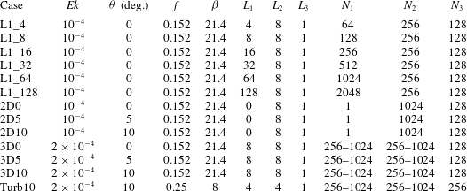
Simulation parameters and case names. Here,
 $L_{i}$
and
 $N_{i}$
represent the length of the domain and the number of computational points respectively in each direction. The Richardson number in all cases is
 $Ri=f^{2}{\it\beta}=0.5$
and
 $Pr=1$
. Multiple grids are used in simulating the bottom four cases to increase the resolution as the flow becomes progressively more nonlinear.

3. Effect of domain size
This study begins with three-dimensional simulations in the same parameter regime as the two-dimensional simulations of Taylor & Ferrari (Reference Taylor and Ferrari2009). Initially, there is a rapid growth of three-dimensional asymmetric modes, but, later in time, the degree of asymmetry decreases. By systematically changing the streamwise domain length,
 $L_{1}$
, we will also show that the dominant instability mode that eventually emerges retains some asymmetry in the case of large
 $L_{1}$
. The initial conditions contain three-dimensional fluctuations in addition to uniform shear and buoyancy gradients. The initial fluctuations are small, containing approximately
 $10^{-6}$
times the total energy contained in the uniform shear. The numerical algorithm uses either second-order central differencing or sixth-order compact differencing on a grid that is staggered in the
 $x_{2}$
and
 $x_{3}$
directions. An in-house parallelized multigrid Poisson solver is used to solve for the pressure deviation,
 $p^{\prime }$
, from the initial balanced pressure every Runge–Kutta substep using either second- or fourth-order finite difference stencils and red–black Jacobi or Gauss–Seidel smoothing. The Navier–Stokes and density equations are evolved using a third-order Runge–Kutta time-marching scheme. Parallelization is accomplished using a message passing interface (MPI). Case-specific computational details are shown in table 1. The two-dimensional simulations use a kinetic energy spectrum of
 $E\propto k^{8}\exp (-4k^{2}/k_{0}^{2})$
, while the three-dimensional cases include only those modes where
 $10k_{h}^{2}\leqslant k_{3}^{2}$
using a spectrum of the form
 $E\propto k^{4}\exp (-2k^{2}/k_{0}^{2})$
. The restriction is introduced to prevent energy from going into large-
 $k_{1}$
modes which are rapidly dissipated in the three-dimensional cases.
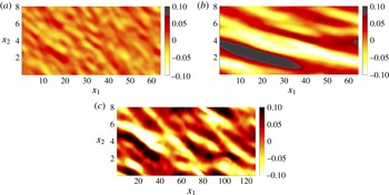
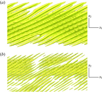
Contours of vertical vorticity
 $({\it\omega}_{3})$
from case L1_64 when (a)
 $t=2.17f^{-1}$
and (b)
 $t=7.09f^{-1}$
along with case L1_128 when (c)
 $t=5.43f^{-1}$
. The cases with smaller
 $L_{1}$
two-dimensionalize (i.e. energy contained primarily in
 $k_{1}=0$
modes) well before
 $t\sim 7f^{-1}$
. Both (b) and (c) were taken immediately preceding the development of strong nonlinearity.

Due to the fact that the dependence on the along-front domain length
 $(L_{1})$
is not known a priori, a range of horizontal aspect ratios
 $(0.5\leqslant L_{1}/L_{2}\leqslant 16)$
were used. In all simulations varying
 $L_{1}$
, the vertical vorticity quickly organized into structures aligned primarily along the horizontal axis tilted approximately
 $45^{\circ }$
asymmetric in the clockwise direction, as illustrated by figure 2(a). The emergence of asymmetric modes for moderate
 $ft$
values is consistent with Mamatsashvili et al. (Reference Mamatsashvili, Vsarlosov, Hagelishvili, Hanishvili and Kalashnik2010). As time progressed, the vertical vorticity gradually reduced its degree of asymmetry and increased in horizontal scale, as seen in figure 2(b). The reduction of asymmetry of the fluctuation modes with increasing time in the simulations is consistent with the linear analysis result of Salhi & Pieri (Reference Salhi and Pieri2014) that asymmetric fluctuations are asymptotically stable as
 $t\rightarrow \infty$
. In all L1_ cases except L1_64 and L1_128 the flow rapidly two-dimensionalizes to purely symmetric (
 $k_{1}=0$
) fluctuations before the development of strong nonlinearity. The time associated with two-dimensionalization increases with increasing
 $L_{1}$
, until cases L1_64 and L1_128, which develop strong nonlinearities before the flow can reach a symmetric state. For structures with a lateral width of
 ${\it\delta}$
, periodicity implies that the smallest asymmetric angle possible is
 ${\it\theta}\sim \tan ^{-1}({\it\delta}/L_{1})$
, indicating that the capture of modes with a small degree of asymmetry requires
 $L_{1}\gg {\it\delta}$
.
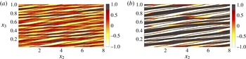
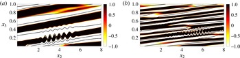
The misalignment of
 ${\it\omega}_{1}$
structures (asymmetric instability currents) with respect to isopycnals throughout the simulation is seen in figure 3. The misalignment becomes less dramatic at later time as the flow becomes more nonlinear and the vortical structure aligns more with the symmetric axis. The reason why large
 $L_{1}$
is needed to capture near-symmetry is due to the periodic boundary conditions in the
 $x_{1}$
direction and the large horizontal scale
 $(k_{h}^{-1})$
of the instability modes. When
 $L_{1}$
is not sufficiently large (e.g. the L1_4, L1_8 and L1_16 cases), then energy rapidly transfers from the
 ${\it\theta}\sim \tan ^{-1}({\it\delta}/L_{1})$
currents to symmetric
 $({\it\theta}=0)$
currents rather than
 ${\it\theta}$
continuing to decrease gradually as in the L1_64 and L1_128 cases. Expanding the analysis of Mamatsashvili et al. (Reference Mamatsashvili, Vsarlosov, Hagelishvili, Hanishvili and Kalashnik2010), § 4 seeks to further explain the evolution of asymmetric flows towards near- as opposed to purely symmetric modes. In the 3D5 and 3D10 cases, the computational domain is rotated about the vertical axis to reduce the
 $L_{1}$
required to capture currents with a small degree of asymmetry.
Contours of along-front vorticity
 $({\it\omega}_{1})$
and isopycnals from case L1_64 when (a)
 $t=2.17f^{-1}$
and (b)
 $t=7.09f^{-1}$
. The cases with
 $L_{1}$
smaller than
 $64$
display far greater alignment between
 ${\it\omega}_{1}$
and isopycnals when
 $t\sim 7f^{-1}$
.

4. Linear stability analysis
Linear stability analysis is employed to understand the evolution of asymmetry of the fluctuations that was described in § 3. Mamatsashvili et al. (Reference Mamatsashvili, Vsarlosov, Hagelishvili, Hanishvili and Kalashnik2010) explored the early transients
 $(t\sim f^{-1})$
, but we are more interested in longer evolution times since secondary instability occurs when
 $t\gg f^{-1}$
in this flow. The base state corresponding to a balanced uniform front is given by
 $$\begin{eqnarray}\langle u_{1}\rangle =Sx_{3}=-\frac{M^{2}}{f}x_{3},\quad \langle {\it\rho}\rangle ={\it\rho}_{0}+\boldsymbol{{\rm\nabla}}_{2}(\langle {\it\rho}\rangle )x_{2}+\boldsymbol{{\rm\nabla}}_{3}(\langle {\it\rho}\rangle )x_{3}.\end{eqnarray}$$
Assuming modes of the form
 ${\it\phi}(t)\exp (\text{i}k_{j}x_{j})$
, one finds that
 $\text{d}k_{3}/\text{d}t=M^{2}k_{1}/f$
as a direct consequence of flow homogeneity. Assuming positive
 $S$
and
 $f$
it follows that
 $M^{2}$
must be negative. Rotating the domain about the vertical axis such that
 $\tan {\it\theta}=k_{1}/k_{2}$
allows for new coordinates such that
 $\tilde{k}_{1}=0$
and
 $\tilde{k}_{2}=k_{h}$
. Under this transformation the symmetric instability corresponds to
 ${\it\theta}=0$
, allowing exploration of the effect of asymmetry by varying
 ${\it\theta}$
. The following linear inviscid governing equations describe motion in the rotated coordinate system:
 $$\begin{eqnarray}\left.\begin{array}{@{}c@{}}\displaystyle \frac{\text{d}u_{1}^{\prime }}{\text{d}t}=fu_{2}^{\prime }+\cos {\it\theta}\frac{M^{2}}{f}u_{3}^{\prime },\quad \frac{\text{d}u_{2}^{\prime }}{\text{d}t}=-fu_{1}^{\prime }-\sin {\it\theta}\frac{M^{2}}{f}u_{3}^{\prime }-\text{i}k_{h}p^{\prime }/{\it\rho}_{0},\\ \displaystyle \frac{\text{d}u_{3}^{\prime }}{\text{d}t}=-\text{i}k_{3}p^{\prime }/{\it\rho}_{0}-g{\it\rho}^{\prime }/{\it\rho}_{0},\quad \frac{\text{d}{\it\rho}^{\prime }}{\text{d}t}\displaystyle =-\text{sin}{\it\theta}\frac{\partial \langle {\it\rho}\rangle }{\partial x_{2}}u_{1}^{\prime }-\cos {\it\theta}\frac{\partial \langle {\it\rho}\rangle }{\partial x_{2}}u_{2}^{\prime }-\frac{\partial \langle {\it\rho}\rangle }{\partial x_{3}}u_{3}^{\prime },\\ \displaystyle 0=\text{i}k_{h}u_{2}^{\prime }+\text{i}k_{3}u_{3}^{\prime }.\end{array}\right\}\end{eqnarray}$$
From continuity, the pressure and vertical velocity variables can be expressed as functions of the other variables. Introducing the buoyancy
 $b^{\prime }=-g{\it\rho}^{\prime }/{\it\rho}_{0}$
, temporarily normalizing all wavenumber components with respect to
 $\Vert \boldsymbol{k}\Vert$
, and introducing the wavevector angle
 ${\it\phi}$
defined by
 $\tan {\it\phi}=k_{h}/k_{3}$
gives the following perturbation evolution equation of the form
 $\text{d}{\it\phi}_{i}^{\prime }/\text{d}t=A_{ij}{\it\phi}_{j}^{\prime }$
:
 $$\begin{eqnarray}\frac{\text{d}}{\text{d}t}\left[\begin{array}{@{}c@{}}u_{1}^{\prime }\\ u_{2}^{\prime }\\ b^{\prime }\end{array}\right]=\left[\begin{array}{@{}ccc@{}}0 & (f\,-\cos {\it\theta}\tan {\it\phi}M^{2}/f) & 0\\ -f\cos ^{2}{\it\phi} & \sin {\it\theta}\sin {\it\phi}\cos {\it\phi}M^{2}/f & -\text{sin}{\it\phi}\cos {\it\phi}\\ -\text{sin}{\it\theta}M^{2} & \tan {\it\phi}N^{2}-\cos {\it\theta}M^{2} & 0\end{array}\right]\left[\begin{array}{@{}c@{}}u_{1}^{\prime }\\ u_{2}^{\prime }\\ b^{\prime }\end{array}\right].\end{eqnarray}$$
The
 $\sin$
terms above grow in influence as the modes become more asymmetric. Taking
 ${\it\theta}=0$
, or for purely symmetric instability, and assuming modes of the form
 $\exp (\text{i}k_{j}x_{j}+{\it\sigma}t)$
one obtains a characteristic equation of the form
 $$\begin{eqnarray}{\it\sigma}^{2}=\cos ^{2}{\it\phi}[M^{4}/N^{2}-f^{2}-N^{2}(\tan {\it\phi}-M^{2}/N^{2})],\end{eqnarray}$$
agreeing with the relation given in Taylor & Ferrari (Reference Taylor and Ferrari2009) for geophysical modes
 $(\cos {\it\phi}\approx 1)$
. As
 $N/f$
increases the range of unstable current slopes
 $(k_{2}/k_{3})$
decreases, peaking at the isopycnal slope.
Reverting back to non-normalized wavenumbers, it is worth noting that
 $k_{3}(t)$
evolves with time,
 $k_{1}$
and
 $k_{2}$
remain fixed at their initial values, and the wavenumber magnitude,
 $k(t)$
, also evolves with time. The time evolutions of the vertical wavenumber (Moffatt Reference Moffatt, Yaglom and Tatarsky1967; Rogallo Reference Rogallo1981) and wavenumber norm are given as
 $$\begin{eqnarray}\frac{\text{d}k_{3}}{\text{d}t}=-Sk_{1}=\frac{M^{2}}{f}k_{1}\quad \text{and}\quad \frac{\text{d}k}{\text{d}t}=\frac{M^{2}}{f}\frac{k_{1}k_{3}}{k}.\end{eqnarray}$$
This implies that the frontal strength, degree of asymmetry and initial alignment of the wavenumber affect how rapidly shear modifies
 $k_{3}/k$
and the underlying mechanism of instability. The non-modal stability problem is solved through introduction of
 $$\begin{eqnarray}\left.\begin{array}{@{}c@{}}\displaystyle \boldsymbol{E}_{ij}^{2}(t)={\it\delta}_{ij}+{\it\delta}_{i2}{\it\delta}_{2j}k_{h}^{2}k_{3}^{-2}(t),\quad \boldsymbol{D}(t)=\left(\frac{\text{d}\boldsymbol{E}(t)}{\text{d}t}+\boldsymbol{E}(t)\boldsymbol{A}(t)\right)\boldsymbol{E}^{-1}(t)\\ \displaystyle \text{and }\unicode[STIX]{x1D731}(T)=\exp \left(\int _{0}^{T}\boldsymbol{D}(t)\,\text{d}t\right).\end{array}\right\}\end{eqnarray}$$
The perturbation energy is given by
 $\Vert \boldsymbol{D}(t){\bf\phi}(t)\Vert ^{2}$
and the perturbation energy growth over period
 $T$
is given by the square of the maximum real eigenvalue of
 $\unicode[STIX]{x1D731}(T)$
.
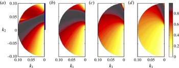
Figure 4 shows the results of the stability analysis, namely the eigenvalues of
 $\unicode[STIX]{x1D731}(T)$
normalized by
 $f$
for SI with
 $Ri=0.5$
, for which one finds
 ${\it\sigma}=f$
. As time increases, a trend of gradually decreasing asymmetry (the black band of high growth rates shifts towards
 $k_{1}=0$
) is found, agreeing with the results of § 3. In these plots it is assumed that
 $k_{3}<0$
, but changing the sign of
 $k_{3}$
simply mirrors the results about the symmetric axis. It should be noted that modes with
 $k_{3}<0$
and
 $k_{1}>0$
have
 $$\begin{eqnarray}\frac{\text{d}{k_{3}}^{2}}{\text{d}t}=\frac{2M^{2}}{f}k_{1}k_{3}>0,\end{eqnarray}$$
since
 $M^{2}<0$
. Thus, the magnitude of
 $k_{3}/k_{2}$
progressively increases and the velocity (perpendicular to the wavenumber) of the associated instability currents becomes more horizontal.
Plots showing the maximum real eigenvalues (normalized by
 $f$
) corresponding to the system of equations
 $\text{d}{\it\phi}_{i}^{\prime }/\text{d}t=A_{ij}{\it\phi}_{j}^{\prime }$
. Growth rates for
 $Ri=0.5$
are shown over various periods given by
 $T=f^{-1}$
(a),
 $2f^{-1}$
(b),
 $4f^{-1}$
(c) and
 $8f^{-1}$
(d). Here, non-dimensional parameters match the regime explored in simulations L1_64 and L1_128. The wavenumber components
 $k_{1}$
and
 $k_{2}$
have been normalized by
 $\Vert \boldsymbol{k}\Vert$
here and
 $k_{3}<0$
initially. The dark vertical line in (a) indicates the symmetric axis.

It is difficult to generate purely symmetric instability when three-dimensional perturbations are allowed because of the stabilization of modes with
 $k_{1}<0$
(right half-plane, not shown in figure 4) by strong stratification. For small negative
 $k_{1}$
, the stabilization of near-symmetric modes is dramatic, with
 $\text{d}k_{3}/\text{d}t=-Sk_{1}\propto -\text{sin}{\it\theta}$
implying a change of sign in
 $\text{d}k_{3}/\text{d}t$
about the symmetric axis. The wavenumbers of these modes, initially with
 $k_{3}<0$
and
 ${\it\theta}<0$
, have
 $\text{d}k_{3}/\text{d}t>0$
and
 $\text{d}k_{3}^{2}/\text{d}t<0$
so that, with increasing time, the magnitude of
 $k_{3}/k_{2}$
progressively decreases and the associated currents become more vertical. Once these currents become more vertical than isopycnals in the frontal zone they are rapidly stabilized by background stratification. Thus, it is not surprising that it is difficult to generate purely symmetric modes in the limit of
 $L_{1}/L_{2}\gg 1$
(e.g. the L1_64 and L1_128 simulations) given that the symmetric axis is nearly the stability boundary for small
 $|\,f|$
and large
 ${\it\beta}=N^{2}/|M^{2}|$
. Decreasing
 $|\,f|$
increases the rate at which currents with
 $k_{1}<0$
become more vertically oriented, while increasing
 ${\it\beta}$
increases the stratification strength.
As
 $f$
is decreased at fixed
 $Ri$
, the stability diagrams do not change appreciably other than modification of the horizontal scale due to change in
 ${\it\beta}$
. Reducing
 $Ri$
to
 $0.3$
results in modes that are less asymmetric, but the general trend in figure 4 is still found. Three-dimensional fluctuations grow at nearly or greater than the symmetric growth rate throughout the range of time scales associated with the development of SI when the strict requirement of
 $k_{1}=0$
is relaxed. Nevertheless, it is because of the tendency for currents to become more aligned with the symmetric axis as time increases that we shift our attention to understanding the development of secondary shear instabilities in symmetric and nearly symmetric flows.
5. Effect of asymmetry
The preceding sections on three-dimensional simulations and linear stability analysis show that fluctuations at late time can take the form of asymmetric modes; the symmetric mode with
 ${\it\theta}=0$
is a special case. Therefore, we further study numerically the influence of non-zero but small
 ${\it\theta}$
on the nonlinear evolution of the flow.
5.1. Two-dimensional simulations
Several two-dimensional simulations were performed in a rotated coordinate system before proceeding to three-dimensional simulations. The first simulation mimicked that of Taylor & Ferrari (Reference Taylor and Ferrari2009) with identical
 $f$
,
 ${\it\beta}$
and
 $\mathit{Ek}$
. The other two simulations are identical except that the computational domain is rotated counterclockwise about the vertical axis by
 $5^{\circ }$
in case 2D5 and
 $10^{\circ }$
in case 2D10 (i.e.
 ${\it\theta}=5^{\circ }$
and
 ${\it\theta}=10^{\circ }$
). This is similar to the rotation of the linear modes in the previous section. In the linear stability analysis, solutions were constant along planes of the form
 $k_{i}x_{i}=C$
and therefore were one-dimensional, varying only in the direction of
 $\boldsymbol{k}$
. These nonlinear two-dimensional simulations allow for fluctuations that are constant along horizontal lines of the form
 $k_{1}x_{1}+k_{2}x_{2}=C$
, where
 $k_{1}=\tan {\it\theta}k_{2}$
. Throughout this and the following sections it is assumed that
 $x_{1}$
and
 $x_{2}$
are in the rotated domain, unless otherwise stated. Due to our interest in nearly symmetric modes (small
 ${\it\theta}$
) the distinction should be minor.
The non-modal stability analysis of § 4 and simulations L1_64 and L1_128 illustrate the tendency for large-scale currents to nearly but not exactly align with the symmetric axis when
 $t\gg f^{-1}$
. Based on the observation that case L1_64 becomes strongly nonlinear when structures are
 $5^{\circ }$
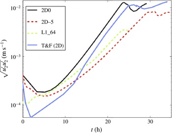
asymmetric, one can compare the two-dimensional symmetric instability growth of perturbations with the asymmetric growth observed in L1_64 and the tilted two-dimensional simulation with
 ${\it\theta}=5^{\circ }$
. Figure 5 shows that the growth of fluctuations in case L1_64 agrees better with the asymmetric two-dimensional simulation (2D5) than the symmetric simulations (2D0 and T&F) after the initial flow adjustment. The reduction in growth relative to the 2D0 case is primarily due to vertical shearing of the asymmetric instability, because the growth rate associated with infinitesimal time (maximal real eigenvalue of
 $\boldsymbol{A}$
from § 4) only reduces to
 $99.3\,\%$
of the symmetric value. The fluctuations initially decay in the two-dimensional simulations in contrast to the three-dimensional cases due to the fact that the three-dimensional instabilities of Mamatsashvili et al. (Reference Mamatsashvili, Vsarlosov, Hagelishvili, Hanishvili and Kalashnik2010) associated with growth over
 $T\sim f^{-1}$
(similarly demonstrated in figure 4) cannot be manifested in the two-dimensional nearly symmetric cases.
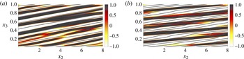
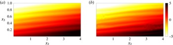
Snapshots of isopycnals and plane-normal vorticity from the symmetric (2D0) and
 ${\it\theta}=10^{\circ }$
(2D10) cases are displayed in figure 6 as the flow becomes nonlinear. The primary distinctions between
 ${\it\theta}=0$
and
 ${\it\theta}=10^{\circ }$
are due to the linear prediction of (4.5). In the asymmetric case, the initial mean shear has a vorticity component in the rotated
 $x_{1}$
coordinate
 $(\langle {\it\omega}_{1}\rangle =\partial \langle u_{2}\rangle /\partial x_{3}=-M^{2}\sin {\it\theta}/f=1.14)$
which continually reduces the vertical inclination of currents, giving rise to currents that are shallower than isopycnals. The increase of
 $|k_{3}|$
by vertical shearing suggests that the vertical length scale,
 ${\it\delta}=2{\it\pi}/k_{3}$
, in the asymmetric cases should be lower than in the symmetric case, but this is not observed because of viscous effects. The viscous growth rate for SI with
 $Ri=0.5$
is given by
 $$\begin{eqnarray}{\it\sigma}/f\sim \sqrt{Ri^{-1}-1}-4{\it\pi}^{2}\mathit{Ek}/{\it\delta}^{2}.\end{eqnarray}$$
Evolution of across-front fluctuations in two-dimensional simulations with varying tilt and a three-dimensional simulation (L1_64) with no tilt and a large along-front domain length. Values from Taylor & Ferrari (Reference Taylor and Ferrari2009) (blue curve) were obtained by digitizing a linear plot, and therefore values are unreliable for
 $\sqrt{u_{2}^{\prime }u_{2}^{\prime }}<10^{-3}~\text{m}~\text{s}^{-1}$
.

Contours of
 ${\it\omega}_{1}$
from two-dimensional simulations where (a)
 ${\it\theta}=0^{\circ }$
and
 $t=6.84f^{-1}$
and (b)
 ${\it\theta}=10^{\circ }$
and
 $t=13.4f^{-1}$
. Isopycnals are also shown by thin solid curves.

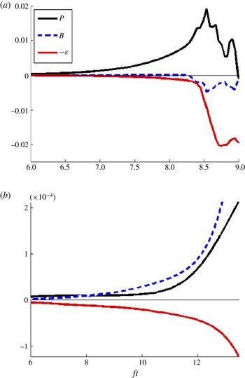
Volume-averaged turbulent kinetic energy budgets from two-dimensional simulations with (a)
 ${\it\theta}=0^{\circ }$
and (b)
 ${\it\theta}=10^{\circ }$
. The difference in magnitudes between cases is due to exponential growth in the symmetric case, while growth is slower in the
 ${\it\theta}=10^{\circ }$
case due to the non-modal nature of instability.

This implies that the growth rates should rapidly drop off (for instance, decrease by more than
 $25\,\%$
) when the vertical scale is
 ${\it\delta}\lesssim 1/8$
for
 $Ri=0.5$
and
 $\mathit{Ek}=10^{-4}$
. The continual shearing due to non-zero
 $\langle {\it\omega}_{1}\rangle$
leads to merging of currents and misalignment with respect to isopycnals, but shearing does not reduce the vertical scale of currents due to currents forming at a scale already marginally influenced by viscosity.
The fluctuation kinetic energy budgets are shown for cases 2D0 and 2D10 in figures 7(a) and 7(b) respectively. The terms contained in the budgets are
 $$\begin{eqnarray}P=-\langle u_{i}^{\prime }u_{j}^{\prime }\rangle \frac{\partial \langle u_{i}\rangle }{\partial x_{j}},\quad B=-\langle u_{3}^{\prime }{\it\rho}^{\prime }\rangle \quad \text{and}\quad {\it\epsilon}=2\mathit{Ek}\langle s_{ij}^{\prime }s_{ij}^{\prime }\rangle .\end{eqnarray}$$
Here,
 $P$
is the shear production,
 $B$
is the buoyancy flux and
 ${\it\epsilon}$
is the viscous dissipation. It takes considerably longer to develop asymmetric currents, as anticipated from the non-modal linear stability analysis for
 $ft\gg 1$
. Buoyancy flux plays a dramatically different role in the two cases, only contributing as a sink after the symmetric case breaks down and being a significant energy source for the asymmetric case.
Isosurface of
 ${\it\lambda}_{2}$
during the development of secondary instability for (a) case 3D0 when
 $t=9.08f^{-1}$
and (b) case 3D10 when
 $t=7.93f^{-1}$
.

5.2. Three-dimensional simulations
In cases 3D0, 3D5 and 3D10 the spatial extent in the
 $x_{1}$
direction is set to
 $8$
, allowing for increased spatial resolution relative to the L1_64 and L1_128 cases at comparable computational cost. This reduced domain size allows for increased resolution of the secondary K–H instability that was first explored in the two-dimensional simulations of Taylor & Ferrari (Reference Taylor and Ferrari2009). In two-dimensional simulations K–H rollers are forced to align with the
 $x_{1}$
direction, unlike in the three-dimensional simulations. Figure 8 shows
 ${\it\lambda}_{2}$
isocontours (Jeong & Hussain Reference Jeong and Hussain1995) capturing coherent vortical structures emerging as a result of secondary K–H instability whose orientation is substantially tilted with respect to the
 $x_{1}$
axis. The emergence of the K–H rollers is most rapid in the symmetric cases, while the wavelength associated with instability decreases as the asymmetry increases. The faster growth rates associated with SI are responsible for the more rapid emergence of localized regions with
 $Ri<0.25$
in the 3D0 case. In figure 9 the development of secondary shear instability is shown for cases 3D0 and 3D10 through vertical slices of
 ${\it\omega}_{1}$
. A slight difference is observed between the slopes of the instability currents, with the 3D10 case yielding shallower slopes than the 3D0 case, as expected.
The coherent secondary K–H rollers are inclined with respect to the
 $x_{1}$
axis, as explained by the following analysis. For symmetric instability (
 $k_{h}/k_{3}={\it\beta}^{-1}$
and
 ${\it\theta}=0$
) the modal stability problem simplifies to an eigenvalue problem of the form
 ${\it\lambda}_{\mathit{max}}{\bf\phi}=\boldsymbol{A}{\bf\phi}$
with
 $b^{\prime }=0$
. Solving for the corresponding eigenvector gives
 $$\begin{eqnarray}\left[\begin{array}{@{}c@{}}u_{1}^{\prime }\\ u_{2}^{\prime }\\ u_{3}^{\prime }\end{array}\right]=\left[\begin{array}{@{}c@{}}\sqrt{(Ri^{-1}-1)(1+{\it\beta}^{-2})}\\ -1\\ {\it\beta}^{-1}\end{array}\right]\exp \left(\text{i}{\it\beta}^{-1}k_{3}x_{2}+\text{i}k_{3}x_{3}+k_{3}\sqrt{Ri^{-1}-1}ft\right),\end{eqnarray}$$
which predicts that SI currents will flow at a horizontal angle significantly tilted with respect to the symmetric axis. In the case of
 $Ri=0.5$
and
 ${\it\beta}^{-2}\ll 1$
, it follows that
 $u_{1}^{\prime }=-u_{2}^{\prime }$
, i.e. an angle of
 $45^{\circ }$
is predicted. Cases 3D0, 3D5 and 3D10 were not able to resolve the intense nonlinearity observed after breakdown of the secondary instability. Section 6 will explore the transition to turbulence of a similar
 $(Ri=0.5)$
front investigated in case Turb10.
Contours of
 ${\it\omega}_{1}$
from three-dimensional simulations showing the development of secondary instabilities where (a)
 ${\it\theta}=0^{\circ }$
and
 $t=8.98f^{-1}$
and (b)
 ${\it\theta}=10^{\circ }$
and
 $t=8.67f^{-1}$
. Isopycnals are also shown by thin solid curves.

6. Frontal turbulence
A three-step process drives the transition from linearly evolving perturbations to turbulence in this flow. The three steps, indicated in figure 14, correspond to secondary instability, tertiary instability and finally three-dimensional turbulence. Before an expanded discussion in §§ 6.1 and 6.2, we provide the following summary of the transition process. During the first step (approximately
 $ft<9$
), the off-SI currents grow in a manner consistent with the linear stability analysis. These modes correspond to vortex sheets that are not aligned with isopycnals and contain primarily
 ${\it\omega}_{1}^{\prime }$
. The vortex sheets become unstable to secondary shear-convective instability at
 $ft\sim 9$
. Early during the secondary instability,
 ${\it\omega}_{2}^{\prime }$
is small and has little to no
 $x_{1}$
dependence. As the secondary instability progresses, the vortex sheets become nonlinear, rapidly rolling up and generating horizontal vorticity fluctuations, increasing both
 ${\it\omega}_{1}^{\prime 2}$
and
 ${\it\omega}_{2}^{\prime 2}$
. Both components increase due to the asymmetric orientation of coherent vortices during the secondary instability. The secondary instability results in the generation of some vertical vorticity fluctuations. However, the mean shear,
 $S=\partial u_{1}/\partial x_{3}$
, of the balanced flow is stable with respect to
 ${\it\omega}_{2}$
fluctuations for
 $Ri=0.5$
, and it is not until the organization in the
 $x_{1}$
–
 $x_{3}$
plane is disrupted through tertiary instabilities, commencing at
 $ft\sim 11$
, that the flow starts to transition to three-dimensional turbulence with significantly large levels of all three components of vorticity fluctuation.
Computational exploration of turbulence in a strong submesoscale front using direct numerical simulation is challenging due largely to the wide range of time scales
 $(S^{\ast }\sim N^{\ast }\gg |M^{\ast }|\gg f^{\ast })$
influencing flow evolution. By increasing
 $f=f^{\ast }/|M^{\ast }|$
from
 $0.152$
to
 $0.25$
and decreasing
 ${\it\beta}=N^{\ast 2}/|M^{\ast 2}|$
from
 $21.4$
to
 $8$
in case Turb10, we are able to reduce
 $S/f$
by a factor of almost three without significantly violating the separation of time scales implicit at frontal regions. Increasing the grid resolution by a factor of two is additionally helpful to fully resolve the secondary shear-convective instabilities which will be discussed in this section. In order to reduce the computational complexity, the size of the domain in each of the horizontal directions is reduced by a factor of two to focus on turbulence rather than merely the evolution of the nearly symmetric currents. In this section,
 $x_{1}$
and
 $x_{2}$
correspond to coordinates in the domain rotated about the vertical axis such that
 $x_{1}$
is aligned with the near-symmetric currents. The angle of rotation is taken to be
 ${\it\theta}=10^{\circ }$
, which is close to the orientation of the primary vortical modes that appeared in lower-resolution three-dimensional simulations.
6.1. Qualitative features
The two distinct features of off-SI not observed in SI are the misalignment of currents and isopycnals and the fact that buoyancy flux is a significant source of fluctuating kinetic energy. These two features are related in the sense that vertical shear drives misalignment which then drives motion across isopycnals, leading to a density variation very similar to that seen in the Turb10 case in figure 10. Unstably stratified regions appear throughout the domain as a result of these slantwise currents. Eventually the shear and unstable density anomaly grow strong enough to lead to secondary instability. The vorticity signature associated with the development of secondary instability (the resulting coherent structures were visualized in figure 8) is shown in figure 11. At this time the two-dimensional assumption appears reasonable, with
 ${\it\omega}_{2}$
in the
 $x_{1}$
–
 $x_{3}$
plane showing nearly no dependence on
 $x_{1}$
. The regions of the density field being strongly stirred in figure 10 coincide with vortex sheets with positive vorticity in figure 11. After this point (i.e.
 $ft>9$
), the secondary instability exhibits weak variability in the
 $x_{1}$
direction.
Vertical snapshots of density variation
 $({\it\rho}-{\it\rho}_{0}={\it\rho}^{\prime }+x_{2}-{\it\beta}x_{3})$
in case Turb10 when
 $t=9f^{-1}$
(a) and
 $t=9.23f^{-1}$
(b) showing density fluctuations immediately preceding and during secondary instability.

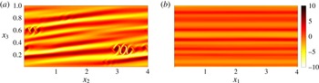
A vertical plane of
 ${\it\omega}_{1}$
from case Turb10 at
 $x_{1}=2$
(a) and a vertical plane of
 ${\it\omega}_{2}$
at
 $x_{2}=2$
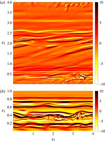
(b) showing horizontal vorticity in case Turb10 during secondary instability at
 $t=9.15f^{-1}$
.

Eventually, the variability in
 ${\it\omega}_{2}$
fluctuations grows sufficiently strong to rapidly destabilize the vertical vorticity field. Figure 12 shows the development of tertiary shear instability once the
 ${\it\omega}_{2}$
fluctuations are strong enough to meander and extract energy from the vertical shear. Prior to this point
 $(ft<10.7)$
, the mean vorticity,
 $\langle {\it\omega}_{2}\rangle =\partial \langle u_{1}\rangle /\partial x_{3}$
, of the original balanced flow was strong relative to the
 ${\it\omega}_{2}$
fluctuations. The secondary shear-convective instability is required to rapidly increase
 ${\it\omega}_{2}$
fluctuations, because the quasi-two-dimensional near-SI currents of the primary instability do not effectively augment
 ${\it\omega}_{2}^{\prime }$
. The flow rapidly three-dimensionalizes after the manifestation of the tertiary instability, destabilizing the balanced flow in the strongly sheared
 $x_{1}$
–
 $x_{3}$
plane. Figure 13 shows
 ${\it\omega}_{1}$
and
 ${\it\omega}_{2}$
vorticity fluctuations as the domain rapidly fills with turbulence. By the end of the simulation, nearly the whole computational domain appears turbulent.
A vertical plane of
 ${\it\omega}_{2}$
from case Turb10 at
 $x_{2}=2$
(b) and a horizontal plane of
 ${\it\omega}_{3}$
at
 $x_{3}=0.5$
(a) when
 $t=10.7f^{-1}$
. Snapshots of horizontal and vertical vorticity are shown when the flow begins to three-dimensionalize.

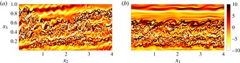
A vertical plane of
 ${\it\omega}_{1}$
from case Turb10 at
 $x_{1}=2$
(a) and a vertical plane of
 ${\it\omega}_{2}$
with
 $x_{2}=2$
(b) at
 $t=11.6f^{-1}$
. Snapshots of horizontal vorticity are taken when strong turbulence fills most of the domain.

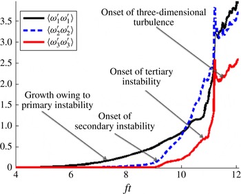
Evolution of volume-averaged fluctuating enstrophy components, showing the development of near-SI followed by secondary instabilities and finally three-dimensional turbulence.

6.2. Quantitative analysis
The nonlinear breakdown to turbulence is rather rapid and proceeds through a three-step process, as was explained in § 6.1. This picture is reinforced quantitatively by figure 14, which shows the evolution of volume-averaged vorticity fluctuations broken down by component. From this plot, times with qualitative changes in vorticity fluctuations can be identified. When
 $ft\sim 9$
, the rate of change of
 ${\it\omega}_{2}^{\prime 2}$
and
 ${\it\omega}_{3}^{\prime 2}$
rapidly increases, corresponding to the emergence of the secondary shear-convective instability. Next, when
 $ft\sim 11$
, the rate of change of
 ${\it\omega}_{1}^{\prime 2}$
and
 ${\it\omega}_{3}^{\prime 2}$
rapidly increases due to tertiary instability. Lastly, when
 $ft\sim 11.2$
, enstrophy shows a sudden decrease followed immediately by growth. It is after
 $ft\sim 11.2$
that the domain fills with small-scale vortical fluctuations and the entire flow becomes turbulent. These results reinforce the notion of three discrete transitional events in the flow which were evident from the instantaneous snapshots of vorticity.
The bulk energetics of the flow are given via turbulent kinetic (introduced in § 5.2) and potential energy budgets in figure 15, with potential energy budget terms defined as
 $$\begin{eqnarray}P_{{\it\rho}}=\langle {\it\rho}^{\prime }u_{2}^{\prime }\rangle ,\quad -B=-{\it\beta}\langle {\it\rho}^{\prime }u_{3}^{\prime }\rangle \quad \text{and}\quad {\it\epsilon}_{{\it\rho}}=\frac{\mathit{Ek}}{Pr}\left\langle \frac{\partial {\it\rho}^{\prime }}{\partial x_{i}}\frac{\partial {\it\rho}^{\prime }}{\partial x_{i}}\right\rangle .\end{eqnarray}$$
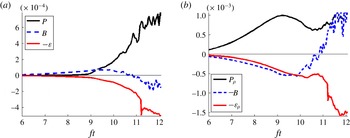
The turbulent kinetic energy budget shows discrete events at
 $ft\sim 9$
when shear production
 $(P)$
switches on as a source,
 $ft\sim 11$
when buoyancy flux
 $(B)$
switches sign to become a sink, and
 $ft=11.2$
when dissipation suddenly jumps. All three are consistent with the observed vorticity dynamics, with
 $P$
switching on due to the onset of secondary shear-convective instability,
 $B$
switching off due to the development of three-dimensionality through tertiary instability and dissipation peaking when the three-dimensional fluctuations develop into small-scale turbulence that fills the domain. The turbulent potential energy budget shows the rate of extraction of energy from potential energy in the front
 $(P_{{\it\rho}})$
, the negative buoyancy flux
 $(-B)$
and potential energy dissipation
 $({\it\epsilon}_{{\it\rho}})$
. Here,
 $P_{{\it\rho}}$
shows a drop following secondary instability and dissipation shows a dramatic ramp-up after the tertiary instability and increases further once the flow is turbulent. The mixing efficiency can be approximated by the ratio of time-integrated
 ${\it\epsilon}_{{\it\rho}}$
to time-integrated
 $P_{{\it\rho}}$
. The turbulent potential energy budget suggests very high mixing efficiency under this definition, and it appears that very efficient mixing would continue in the turbulent regime. Comparing the magnitudes of
 ${\it\epsilon}_{{\it\rho}}$
and
 ${\it\epsilon}+{\it\epsilon}_{{\it\rho}}$
also suggests a high mixing efficiency, taking values of roughly
 $75\,\%$
in the turbulent regime.
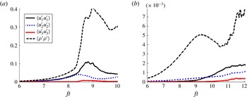
Figure 16 shows the evolution of turbulence energetics in cases 2D0 and Turb10. A much larger proportion of energy is contained within the density fluctuations early in the evolution of Turb10. This is consistent with the misalignment of near-symmetric currents extracting available potential energy from the front. A reduction in
 $\langle {\it\rho}^{\prime }{\it\rho}^{\prime }\rangle$
is observed during the period of shear-convective secondary instability when
 $9\lesssim ft\lesssim 11$
. The amplitude of vertical velocity fluctuations relative to the horizontal fluctuations in the three-dimensional case is not nearly as small as in the two-dimensional case. It is also worth noting that the two-dimensional case develops unrealistically large fluctuation amplitudes compared with the three-dimensional turbulent case.
Terms from the volume-averaged turbulent kinetic energy (a) and turbulent potential energy (b) budgets throughout the duration of case Turb10.

Volume-averaged energetics throughout the duration of cases 2D0 (a) and Turb10 (b).

7. Conclusion
This study explores the development of instability and turbulence in a symmetrically unstable variant of Eady’s model with
 $Ri=0.5$
. The novelty of the approach is the simulation of fully three-dimensional turbulence in a baroclinic flow with boundaries that is unstable to symmetric instability. The flow progresses through a sequence of instabilities whose effect is quantified, e.g. the temporal evolution of volume-averaged vorticity fluctuations in figure 14. Linear stability analysis is also performed to understand and interpret three-dimensional effects which are manifested not only in transition to turbulence but also during the initial evolution of small-amplitude three-dimensional disturbances.
The initial vertical vorticity fluctuations organize into structures that are inclined at approximately
 $-45^{\circ }$
in the
 $x_{1}$
–
 $x_{2}$
plane and instability currents that are misaligned with respect to the isopycnals. This behaviour for
 $ft=\mathit{O}(1)$
is consistent with the results of Mamatsashvili et al. (Reference Mamatsashvili, Vsarlosov, Hagelishvili, Hanishvili and Kalashnik2010). As time advances, the horizontal scale of the flow continually increases, especially in the along-front direction, and the flow tends towards two-dimensionality. However, for sufficiently large horizontal domains, nonlinearity emerges for currents that, although near-symmetric (the angle
 ${\it\theta}$
between the current and the symmetric axis is roughly
 $5^{\circ }$
in the largest-domain case), are not exactly symmetric. In other words, it is the asymmetric instability that evolves nonlinearly rather than the purely symmetric (
 $k_{1}=0$
) instability. The sensitivity of this finding of nonlinearly evolving asymmetric instability to the choice of initial conditions for the fluctuations (the horizontal length scale is larger than the vertical length scale in the present case, as in geophysical flows) and the Reynolds number is worth exploring in future three-dimensional studies.
Non-modal linear stability analysis showed a tendency for the flow to nearly align with the symmetric axis once
 $ft\gg 1$
for strong shear
 $(|S/f|\gg 1)$
and stratification
 $(|N/f|\gg 1)$
. The vertical scale of the observed asymmetric modes decreases with time, resulting in misalignment of asymmetric currents and isopycnals. The analysis shows that vertical shear stabilizes nearly symmetric modes tilted in the direction opposite to that observed in the simulations, explaining why the oppositely tilted modes do not amplify in the simulations. For these modes,
 $k_{3}/k_{2}$
decreases in magnitude with time, leading to currents that are steeper than the isopycnal slope, resulting in rapid suppression. It is because of these issues that the analysis of purely symmetric instability through two-dimensional simulations may not be appropriate for frontal zones with strong lateral density gradients and vertical shear.
The computational domains are rotated about the vertical axis to investigate near-symmetric currents in both the linear stability analysis and numerical simulations. A two-dimensional simulation rotated to be nearly aligned with the
 $5^{\circ }$
asymmetric currents found in the three-dimensional direct numerical simulation displayed perturbation growth rates similar to those seen in the three-dimensional simulation. Misalignment of asymmetric currents and isopycnals allows currents to be strengthened by both the reservoir of kinetic energy in the vertical shear and the reservoir of potential energy in the density front, simultaneously. The secondary shear instability is misaligned with the symmetric axis, implying that two-dimensional simulations are unable to accurately capture secondary shear instabilities in both symmetric and asymmetric currents.
Finally, the forward cascade from balanced vertical shear to turbulence is demonstrated using a high-resolution simulation with the computational domain rotated about the vertical axis by
 $10^{\circ }$
. The quiescent flow develops a primary instability that takes the form of nearly two-dimensional asymmetric currents. When the perturbations become large during the transient growth period, there is a secondary (originating in the
 $y$
–
 $z$
plane where
 $y$
is the cross-front direction and
 $z$
is vertical) shear-convective instability. Another important transition event related to a tertiary instability (see figure 14) occurs later, and is not present in two-dimensional simulations. The balanced base flow has mean shear flow,
 $\langle u_{1}\rangle (x_{3})$
, that is stable to
 ${\it\omega}_{2}$
fluctuations for
 $Ri=0.5$
. During the tertiary instability, lateral vorticity fluctuations
 $({\it\omega}_{2}^{\prime })$
grow large enough for nonlinearity to overcome the organization of the balanced base flow, enhancing extraction of kinetic energy from the shear. This transition leads to fully three-dimensional vortical flow which rapidly becomes more multiscale until three-dimensional well-developed shear-driven turbulence emerges. The mixing of the density field
 $({\it\epsilon}_{{\it\rho}})$
is strong and increases by a factor of three after the destabilization of the shearing plane, which is also not present in two-dimensional simulations.
Acknowledgements
The authors are grateful for computational resources through a research allocation through the Extreme Science and Engineering Discovery Environment (XSEDE) and for the detailed helpful comments of the reviewers.