1. Introduction
During the last few decades, the microscopic and macroscopic properties of granular materials have been studied under different physical conditions (Goldhirsch Reference Goldhirsch2003; Forterre & Pouliquen Reference Forterre and Pouliquen2008). One extreme state of driven granular materials is a granular gas (Pöschel & Luding Reference Pöschel and Luding2001), which can be realized under strong external driving (such as shaking), but it differs from a molecular gas in that the macroscopic particles collide inelastically, resulting in a loss of kinetic energy (
 ${\sim}(1-{\it\alpha}^{2})$
, where
 $0\leqslant {\it\alpha}\leqslant 1$
is the coefficient of restitution). Granular gases fall under the category of rapid flows, which are well described by hydrodynamic-like equations. The coarse-graining of the pertinent ‘inelastic’ Boltzmann equation results in Euler- and Navier–Stokes-type equations, modified to account for inelastic dissipation that appears as an extra term in the energy equation. Such hydrodynamic equations have been employed to understand the dynamics of granular fluids in different flow configurations (vibrated bed, Couette flow, Chute flow, etc.) up to a moderate density. One noteworthy feature of rapid granular flows is that they can be supersonic (Haff Reference Haff1983), and shock waves form even under normal conditions (e.g. flow around obstacles (Buchholtz & Pöschel Reference Buchholtz and Pöschel1998; Rericha et al.
Reference Rericha, Bizon, Shattuck and Swinney2002; Amarouchene & Kellay Reference Amarouchene and Kellay2006; Boudet, Amarouchene & Kellay Reference Boudet, Amarouchene and Kellay2008), strong shaking (Bougie et al.
Reference Bougie, Moon, Swift and Swinney2002; Carrillo, Pöschel & Saluena Reference Carrillo, Pöschel and Saluena2008) and shallow free-surface flows (Gray, Tai & Noelle Reference Gray, Tai and Noelle2003)).
A plane shock wave is generated when a supersonic gas flows into a subsonic gas; mathematically, this is nothing but a discontinuity across which the hydrodynamic fields undergo discontinuous jumps (Courant & Friedrichs Reference Courant and Friedrichs1948). The simplest nonlinear equation that admits shock solutions is the inviscid Burger equation, which represents a nonlinear ‘hyperbolic’ equation; a hyperbolic system in an infinite domain (
 $-\infty <x<-\infty$
) with discontinuous initial conditions constitutes the ‘Riemann problem’ of shock waves (Courant & Friedrichs Reference Courant and Friedrichs1948; Prasad Reference Prasad2001). From an experimental viewpoint, the Riemann problem can be mimicked by the one-dimensional version of the shock-tube problem, which comprises a gas-filled long tube separated into two chambers by a membrane. The gases in the two chambers are in equilibrium, but differ in pressure and density. After the membrane is burst, a shock wave and a contact discontinuity travel into the low-pressure region of the tube at supersonic speeds and a rarefaction wave travels in the opposite direction. Apart from its interesting physical properties, the shock-tube problem also serves as a standard benchmark to check (i) the accuracy of gas dynamics models as well as (ii) the robustness of the numerical scheme to reproduce the shock profiles. The analogous Riemann problem of ‘granular’ shock waves is interesting in its own right and might be helpful for a better understanding of macroscopic properties of granular gases as well as to check the validity of adopted hydrodynamic equations (Haff Reference Haff1983; Jenkins & Savage Reference Jenkins and Savage1983; Goldshtein & Shapiro Reference Goldshtein and Shapiro1995; Esipov & Pöschel Reference Esipov and Pöschel1997; Sela & Goldhirsch Reference Sela and Goldhirsch1998; Garzo, Santos & Montanero Reference Garzo, Santos and Montanero2007; Saha & Alam Reference Saha and Alam2014).
In previous works on plane shock waves in granular gases (Goldshtein et al. Reference Goldshtein, Shapiro, Moldavsky and Fichman1995; Kamenetsky et al. Reference Kamenetsky, Goldshtein, Shapiro and Degani2000), the Euler-level hydrodynamic equations, with dense-gas corrections for pressure and inelastic dissipation, were employed to analyse the well-known ‘piston’ problem: a rigid piston moves through an undisturbed granular gas with a constant velocity, resulting in a steadily propagating shock front. Specific assumptions were made on the state of the gas adjacent to the piston, yielding a ‘solid’ region (with maximum density and zero granular temperature) next to the piston that coexisted with a non-uniform region having a propagating shock front at the downstream end. The primary motivation of these works was to understand a possible relation between the transport of mass and energy in a vertically vibrated bed of granular material and the shock-wave propagation through the bed. Later works (Bougie et al. Reference Bougie, Moon, Swift and Swinney2002; Carrillo et al. Reference Carrillo, Pöschel and Saluena2008) investigated the role of shock-wave propagation on the ‘pattern-formation’ scenario in a vertically vibrated bed by solving the Navier–Stokes-order equations but supplemented with boundary conditions. Derivation/postulation of the correct forms of boundary conditions still remains an active field of research (Nott Reference Nott2011) in rapid granular flows.
Leaving aside boundary effects, here we analyse the plane shock waves propagating in an unbounded granular gas, which, to the best of our knowledge, have not been studied before. The supersonic and subsonic granular gases are taken as the left and right states, separated by a discontinuity whose time evolution is analysed (§ 2). We solve the Euler and Navier–Stokes equations of a dilute granular gas using a relaxation-type numerical scheme (§ 3). Our primary focus is to identify the structural features of the granular shock profiles (of density, temperature and velocity, § 4) and contrast them with those of an ideal molecular gas. In addition, the validity of Haff’s law (Haff Reference Haff1983) is critically assessed in the presence of a shock wave, and certain scaling relations are uncovered. The large-time evolution of the shock profiles is briefly discussed in § 4.2.3.
2. Hydrodynamic equations for a granular gas and plane shock waves
We consider a dilute granular gas of smooth inelastic spheres of mass
 $m$
and diameter
 $d$
that interact via binary collisions. The macroscopic variables, namely the mass density
 ${\it\rho}$
, the hydrodynamic velocity
 $\boldsymbol{u}$
and the granular/kinetic temperature
 ${\it\theta}$
, are obtained via a coarse-graining procedure over the distribution function
 $\mathit{f(\boldsymbol{v}, \boldsymbol{x}, t)}$
:
 $$\begin{eqnarray}{\it\rho}=\int mf\,\text{d}\boldsymbol{v}\equiv mn,\quad {\it\rho}u_{i}=\int mv_{i}\,f\,\text{d}\boldsymbol{v},\quad {\it\theta}=\frac{1}{3n}\int C^{2}f\,\text{d}\boldsymbol{v},\end{eqnarray}$$
where
 $\boldsymbol{C}=(\boldsymbol{v}-\boldsymbol{u})$
is the peculiar velocity and
 $n$
is the number density. At Navier–Stokes (NS) order, other relevant moments are the pressure tensor
 $\unicode[STIX]{x1D631}_{ij}$
and the heat flux vector
 $q_{i}$
:
 $$\begin{eqnarray}\unicode[STIX]{x1D631}_{ij}=\int mC_{i}C_{j}\;f\,\text{d}\boldsymbol{v}\equiv \unicode[STIX]{x1D631}{\it\delta}_{ij}+{\it\sigma}_{ij},\quad q_{i}=\int \frac{m}{2}C^{2}C_{i}\,f\,\text{d}\boldsymbol{v}.\end{eqnarray}$$
The pressure tensor is decomposed such that
 $\unicode[STIX]{x1D665}={\it\rho}{\it\theta}$
is the pressure and
 ${\it\sigma}_{ij}$
is its deviatoric part.
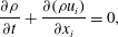
The hydrodynamic balance equations for the mass, momentum and energy can be written as
 $$\begin{eqnarray}\displaystyle & \displaystyle \frac{\partial {\it\rho}}{\partial t}+\frac{\partial ({\it\rho}u_{i})}{\partial x_{i}}=0, & \displaystyle\end{eqnarray}$$
 $$\begin{eqnarray}\displaystyle & \displaystyle \frac{\partial ({\it\rho}u_{i})}{\partial t}+\frac{\partial ({\it\rho}u_{i}u_{j})}{\partial x_{j}}+\frac{\partial p}{\partial x_{i}}+\frac{\partial {\it\sigma}_{ij}}{\partial x_{j}}=0, & \displaystyle\end{eqnarray}$$
 $$\begin{eqnarray}\displaystyle & \displaystyle \frac{3}{2}\frac{\partial p}{\partial t}+\frac{3}{2}\frac{\partial (pu_{i})}{\partial x_{i}}+\frac{\partial q_{i}}{\partial x_{i}}+p\frac{\partial u_{i}}{\partial x_{i}}+{\it\sigma}_{ij}\frac{\partial u_{i}}{\partial x_{j}}=-\frac{3}{2}\mathscr{D}. & \displaystyle\end{eqnarray}$$
 $$\begin{eqnarray}\mathscr{D}=\frac{4}{3}nd^{2}\sqrt{{\rm\pi}}(1-{\it\alpha}^{2})\left(1+\frac{3}{16}a_{2}\right){\it\rho}{\it\theta}^{3/2},\quad \text{with }a_{2}=\frac{16(1-{\it\alpha})(1-2{\it\alpha}^{2})}{30{\it\alpha}^{2}(1-{\it\alpha})+81-17{\it\alpha}}\end{eqnarray}$$
representing the contracted fourth moment of the distribution function. The set of balance equations (2.3)–(2.5) is made closed by providing constitutive relations for
 ${\it\sigma}_{ij}$
and
 $q_{i}$
:
 $$\begin{eqnarray}{\it\sigma}_{ij}=-2{\it\mu}\left(\frac{1}{2}\left(\frac{\partial u_{i}}{\partial x_{j}}+\frac{\partial u_{i}}{\partial x_{i}}\right)-\frac{1}{3}\frac{\partial u_{i}}{\partial x_{i}}\right)\quad \text{and}\quad q_{i}=-{\it\kappa}\frac{\partial {\it\theta}}{\partial x_{i}}-{\it\kappa}_{h}\frac{\partial {\it\rho}}{\partial x_{i}}.\end{eqnarray}$$
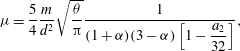
The simplified expressions for the shear viscosity
 ${\it\mu}$
, the thermal conductivity
 ${\it\kappa}$
and the higher-order thermal conductivity
 ${\it\kappa}_{h}$
are given by (Garzo et al.
Reference Garzo, Santos and Montanero2007; Kremer & Marques Reference Kremer and Marques2011)
 $$\begin{eqnarray}\displaystyle & \displaystyle {\it\mu}=\frac{5}{4}\frac{m}{d^{2}}\sqrt{\frac{{\it\theta}}{{\rm\pi}}}\frac{1}{(1+{\it\alpha})(3-{\it\alpha})\left[1-\displaystyle \frac{a_{2}}{32}\right]}, & \displaystyle\end{eqnarray}$$
 $$\begin{eqnarray}\displaystyle & \displaystyle {\it\kappa}=\frac{75}{2}\frac{m}{d^{2}}\sqrt{\frac{{\it\theta}}{{\rm\pi}}}\frac{(1+2a_{2})}{(1+{\it\alpha})\left[49-33{\it\alpha}+(19-3{\it\alpha})\displaystyle \frac{a_{2}}{32}\right]}, & \displaystyle\end{eqnarray}$$
 $$\begin{eqnarray}\displaystyle & \displaystyle {\it\kappa}_{h}=\frac{75}{2{\it\rho}}\frac{m}{d^{2}}{\it\theta}\sqrt{\frac{{\it\theta}}{{\rm\pi}}}\frac{a_{2}}{(1+{\it\alpha})\left[49-33{\it\alpha}+(19-3{\it\alpha})\displaystyle \frac{a_{2}}{32}\right]}. & \displaystyle\end{eqnarray}$$
 $$\begin{eqnarray}{\it\sigma}_{ij}=0=q_{i}.\end{eqnarray}$$
It may be noted that the hydrodynamic equations for a molecular gas remain the same as (2.3)–(2.5), but the restitution coefficient is set to
 ${\it\alpha}=1$
such that the collisional dissipation (2.6) in the energy (2.5) vanishes identically (i.e.
 $\mathscr{D}=0=a_{2}$
). Moreover, the transport coefficients (2.8)–(2.10) are also taken as those for perfectly elastic collisions,
 ${\it\mu}\equiv {\it\mu}({\it\alpha}=1)$
,
 ${\it\kappa}\equiv {\it\kappa}({\it\alpha}=1)$
and
 ${\it\kappa}_{h}\equiv 0$
; these are used to calculate the shock profiles in a molecular gas, as discussed in § 4.1.
2.1. Equations for plane shock waves: Navier–Stokes and Euler models
For planar shock waves propagating along the
 $x$
-direction, all variables are functions of a single spatial coordinate
 $x$
and time
 $t$
; the system is assumed to be uniform (having no gradients) and infinite along the
 $y$
- and
 $z$
-directions. The flow velocity and heat flux in the
 $x$
-direction are denoted by
 $u(x,t)$
and
 $q(x,t)$
respectively, and they are zero in the two remaining (
 $y$
and
 $z$
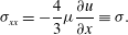
) orthogonal directions. It is straightforward to verify that the deviatoric stress tensor has one non-zero component, the ‘longitudinal’ stress, which can be expressed as
 $$\begin{eqnarray}{\it\sigma}_{xx}=-\frac{4}{3}{\it\mu}\frac{\partial u}{\partial x}\equiv {\it\sigma}.\end{eqnarray}$$
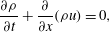
With the above definitions, the one-dimensional balance equations for the Navier–Stokes (NS) model can be written in ‘quasiconservation’ form,
 $$\begin{eqnarray}\displaystyle & \displaystyle \frac{\partial {\it\rho}}{\partial t}+\frac{\partial }{\partial x}({\it\rho}u)=0, & \displaystyle\end{eqnarray}$$
 $$\begin{eqnarray}\displaystyle & \displaystyle \frac{\partial }{\partial t}({\it\rho}u)+\frac{\partial }{\partial x}({\it\rho}u^{2}+{\it\rho}{\it\theta}+{\it\sigma})=0, & \displaystyle\end{eqnarray}$$
 $$\begin{eqnarray}\displaystyle & \displaystyle \frac{\partial }{\partial t}({\it\rho}u^{2}+3{\it\rho}{\it\theta})+\frac{\partial }{\partial x}({\it\rho}u^{3}+5{\it\rho}{\it\theta}u+2u{\it\sigma}+2q)=-3\mathscr{D}, & \displaystyle\end{eqnarray}$$
 $\mathscr{D}$
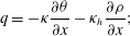
in the energy equation (2.15). The constitutive relation for the heat flux is
 $$\begin{eqnarray}q=-{\it\kappa}\frac{\partial {\it\theta}}{\partial x}-{\it\kappa}_{h}\frac{\partial {\it\rho}}{\partial x};\end{eqnarray}$$
the longitudinal stress
 ${\bf\sigma}$
and the dissipation rate
 $\mathscr{D}$
are given by (2.12) and (2.6) respectively. The one-dimensional Euler system is obtained by setting
 ${\it\sigma}=0$
and
 $q=0$
in (2.13)–(2.15).
2.2. Rankine–Hugoniot conditions of a granular gas and the end states
Let us denote the upstream (
 $x\rightarrow -\infty$
) and downstream (
 $x\rightarrow \infty$
) states of a shock, located at
 $x=0$
, by
 $({\it\rho}_{1},u_{1},{\it\theta}_{1})$
and
 $({\it\rho}_{2},u_{2},{\it\theta}_{2})$
respectively. The finite jump in each state variable across a shock is given by the so-called Rankine–Hugoniot (RH) relations (Courant & Friedrichs Reference Courant and Friedrichs1948), which connect the upstream and downstream states of a shock. These relations can be obtained from the balance laws (2.13)–(2.15) by using the fact that the terms that are independent of the gradients of the hydrodynamic fields do not contribute (see § 63 in Courant & Friedrichs Reference Courant and Friedrichs1948):
 $$\begin{eqnarray}\displaystyle & \displaystyle {\it\rho}_{1}v_{1}={\it\rho}_{2}v_{2}, & \displaystyle\end{eqnarray}$$
 $$\begin{eqnarray}\displaystyle & \displaystyle {\it\rho}_{1}v_{1}^{2}+{\it\rho}_{1}{\it\theta}_{1}+{\it\sigma}_{1}={\it\rho}_{2}v_{2}^{2}+{\it\rho}_{2}{\it\theta}_{2}+{\it\sigma}_{2}, & \displaystyle\end{eqnarray}$$
 $$\begin{eqnarray}\displaystyle & \displaystyle {\it\rho}_{1}v_{1}^{3}+5{\it\rho}_{1}{\it\theta}_{1}v_{1}+2{\it\sigma}_{1}v_{1}+2q_{1}={\it\rho}_{2}v_{2}^{3}+5{\it\rho}_{2}{\it\theta}_{2}v_{2}+2{\it\sigma}_{2}v_{2}+2q_{2}, & \displaystyle\end{eqnarray}$$
 $v_{i}=u_{i}-v_{sh}$
, with
 $v_{sh}$
being the shock speed. An additional ansatz is now made: the upstream and downstream states are spatially uniform (which, along with a temporally decaying temperature field, represents the ‘local’ equilibrium of a granular gas (Haff Reference Haff1983), known as the homogeneous cooling state, see (4.3) in § 4.2.2). The spatial homogeneity (i.e.
 $\boldsymbol{{\rm\nabla}}({\it\rho},\boldsymbol{u},{\it\theta})=0$
) of end states implies that the flux terms
 ${\it\sigma}$
, (2.12), and
 $q$
, (2.16), vanish at
 $x\rightarrow \pm \infty$
. Therefore, putting
 ${\it\sigma}=0=q$
into (2.17)–(2.19) we arrive at the RH conditions for a granular gas. It may be noted that the resulting RH conditions are identical for both molecular and ‘smooth’ granular gases (Goldshtein et al.
Reference Goldshtein, Shapiro, Moldavsky and Fichman1995) at the Euler/NS order of hydrodynamics.
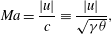
The local Mach number
 $Ma$
is defined as the ratio of the velocity of the gas to the speed of sound through the granular gas,
 $$\begin{eqnarray}Ma=\frac{|u|}{c}\equiv \frac{|u|}{\sqrt{{\it\gamma}{\it\theta}}},\end{eqnarray}$$
where
 ${\it\gamma}=5/3$
is the adiabatic index (the ratio between two specific heats), whose numerical value for a monatomic granular gas (Goldshtein & Shapiro Reference Goldshtein and Shapiro1995; Amarouchene & Kellay Reference Amarouchene and Kellay2006) is the same as for a molecular gas, and
 $c=\sqrt{{\it\gamma}{\it\theta}}$
is the adiabatic sound speed, which is also the characteristic slope (Courant & Friedrichs Reference Courant and Friedrichs1948) obtained from the Euler equations.
The initial (
 $t=0$
) shock profiles are given by (
 ${\it\rho}_{1},u_{1},{\it\theta}_{1}$
) for
 $x\leqslant 0$
and (
 ${\it\rho}_{2},u_{2},{\it\theta}_{2}$
) for
 $x>0$
, and the shock speed is zero at
 $t=0$
. Assuming that the flow is adiabatic and solving the RH relations (2.17)–(2.19) for a stationary shock, the downstream quantities can be expressed in terms of their upstream counterparts,
 $$\begin{eqnarray}\frac{{\it\rho}_{2}}{{\it\rho}_{1}}=\frac{({\it\gamma}+1)Ma_{1}^{2}}{2+({\it\gamma}-1)Ma_{1}^{2}}\equiv \frac{u_{1}}{u_{2}},\quad \frac{{\it\theta}_{2}}{{\it\theta}_{1}}=\frac{(2{\it\gamma}Ma_{1}^{2}-({\it\gamma}-1))(({\it\gamma}-1)Ma_{1}^{2}+2)}{({\it\gamma}+1)^{2}Ma_{1}^{2}},\end{eqnarray}$$
where
 $Ma_{1}=|u_{1}|/\sqrt{{\it\gamma}{\it\theta}_{1}}$
is the upstream Mach number.
3. Dimensionless equations and the numerical scheme
3.1. Reference scales and dimensionless equations
One should be careful in choosing the reference scales for non-dimensionalization, since, unlike in an equilibrium molecular gas, the hydrodynamic fields in a granular gas can vary with time. We use all ‘upstream’ state quantities evaluated at
 $t=0$
as reference scales for non-dimensionalization. The dimensionless variables are therefore given by
 $$\begin{eqnarray}\hat{{\it\rho}}=\frac{{\it\rho}}{{\it\rho}_{1}(0)},\quad \hat{u} =\frac{u}{\sqrt{{\it\theta}_{1}(0)}},\quad \hat{{\it\theta}}=\frac{{\it\theta}}{{\it\theta}_{1}(0)},\quad \hat{{\it\sigma}}=\frac{{\it\sigma}}{{\it\rho}_{1}{\it\theta}_{1}(0)},\quad \hat{x}=\frac{x}{l_{1}},\quad \hat{t}=\frac{t\sqrt{{\it\theta}_{1}(0)}}{l_{1}},\vphantom{\mathop{\sum }_{a}}\end{eqnarray}$$
where the length scale used is the mean free path,
 $l=16{\it\mu}/5\sqrt{2{\rm\pi}}{\it\rho}\sqrt{{\it\theta}}$
, with the shear viscosity
 ${\it\mu}$
being given by (2.8).
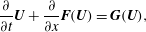
The one-dimensional balance equations in dimensionless form have the same form as in (2.13)–(2.15), which can be written in operator form (removing the hat from dimensionless quantities)
 $$\begin{eqnarray}\frac{\partial }{\partial t}\boldsymbol{U}+\frac{\partial }{\partial x}\boldsymbol{F}(\boldsymbol{U})=\boldsymbol{G}(\boldsymbol{U}),\end{eqnarray}$$
where
 $\boldsymbol{U}=({\it\rho},{\it\rho}u,{\it\rho}u^{2}+3{\it\rho}{\it\theta})^{\text{T}}$
is the vector of variables,
 $\boldsymbol{F}(\boldsymbol{U})=({\it\rho}u,{\it\rho}u^{2}+{\it\rho}{\it\theta},{\it\rho}u^{3}+5{\it\rho}{\it\theta}u)^{\text{T}}$
is the vector of flux and
 $\boldsymbol{G}(\boldsymbol{U})$
is the vector of source terms (i.e. the remaining terms of (2.13)–(2.15)). The system (3.2) is called hyperbolic in
 $\boldsymbol{U}$
and
 $t$
if the eigenvalues of the Jacobian matrix,
 $\partial \boldsymbol{F}(\boldsymbol{U})/\partial \boldsymbol{U}$
, are real and distinct (Courant & Friedrichs Reference Courant and Friedrichs1948), and hence the characteristic speeds are finite.
3.2. Relaxation-type numerical scheme
An appropriate shock-capturing scheme (LeVeque Reference LeVeque2002) needs to be employed to solve (3.2) along with Rankine–Hugoniot conditions (2.21). We adapt the relaxation scheme of Jin & Xin (Reference Jin and Xin1995) to the present problem. The solution of (3.2) involves a ‘two-stage’ procedure: in the first stage, the homogeneous equation
 $$\begin{eqnarray}\frac{\partial \boldsymbol{U}^{h}}{\partial t}+\frac{\partial \boldsymbol{F}(\boldsymbol{U}^{h})}{\partial x}=0,\quad \text{with }\boldsymbol{U}^{h}(x,t=0)=\boldsymbol{U}(x,t=0),\end{eqnarray}$$
is solved, and in the second stage, the solution of the homogeneous part (3.3) is used to solve
 $$\begin{eqnarray}\frac{\partial \boldsymbol{U}}{\partial t}=\boldsymbol{G}(\boldsymbol{U}),\quad \text{with }\boldsymbol{U}(x,t=0)=\boldsymbol{U}^{h}(x,t=0),\end{eqnarray}$$
and thereby construct the full solution.
The homogeneous system (3.3) is solved by finding the solution of an equivalent relaxation system (Jin & Xin Reference Jin and Xin1995)
 $$\begin{eqnarray}\displaystyle & \displaystyle \frac{\partial \boldsymbol{U}}{\partial t}+\frac{\partial \boldsymbol{V}}{\partial x}=0, & \displaystyle\end{eqnarray}$$
 $$\begin{eqnarray}\displaystyle & \displaystyle \frac{\partial \boldsymbol{V}}{\partial t}+\unicode[STIX]{x1D63C}\frac{\partial \boldsymbol{U}}{\partial x}=-\frac{1}{{\it\epsilon}}(\boldsymbol{V}-\boldsymbol{F}(\boldsymbol{U})), & \displaystyle\end{eqnarray}$$
 $\boldsymbol{U}\in \mathbb{R}^{n}$
,
 $\boldsymbol{V}\in \mathbb{R}^{n}$
,
 $(x,t)\in \mathbb{R}\times \mathbb{R}_{+}$
and
 ${\it\epsilon}$
is a small positive parameter called the relaxation rate. Putting
 ${\it\epsilon}\rightarrow 0$
in (3.6), we obtain the local equilibrium solution
 $\boldsymbol{V}=\boldsymbol{F}(\boldsymbol{U})$
, which, along with (3.5), retrieves the original equation (3.3). In (3.6),
 $$\begin{eqnarray}\unicode[STIX]{x1D63C}=\text{diag}\{a_{1},a_{2},\ldots ,a_{n}\},\quad a_{m}>0~(1\leqslant m\leqslant n),\end{eqnarray}$$
is a diagonal matrix that must be appropriately chosen. The Jacobian matrix of flux
 $\boldsymbol{F}(\boldsymbol{U})$
constitutes a ‘complete’ eigensystem
 $({\it\lambda}_{1},{\it\lambda}_{2},\ldots ,{\it\lambda}_{n})$
, and we choose
 $a_{1}=\cdots =a_{n}=\max (\sup |{\it\lambda}_{1}|,\ldots ,\sup |{\it\lambda}_{n}|)$
to construct the diagonal matrix (3.7a,b
).
For spatial discretization, uniform grid points with a step size of
 ${\rm\Delta}x$
are used; the time discretization is also taken as uniform with a time step of
 ${\rm\Delta}t$
. A first-order accurate upwind scheme for spatial discretization and a second-order TVD (total variation diminishing) Runge–Kutta time-splitting scheme (which consists of a sequence of implicit–explicit time steps) are applied to the system (3.5)–(3.6); the specific details of the algorithm can be found in Jin & Xin (Reference Jin and Xin1995). Once the solution of the homogeneous part
 $\boldsymbol{U}_{i}^{(h)}$
is known, we can find the solution
 $\boldsymbol{U}_{i}$
of (3.4),
 $$\begin{eqnarray}\boldsymbol{U}_{i}=\boldsymbol{U}_{i}^{(h)}+{\rm\Delta}t\,\boldsymbol{G}(\boldsymbol{U}_{i}^{(h)}).\end{eqnarray}$$
The spatial (
 ${\rm\Delta}x$
) and temporal (
 ${\rm\Delta}t$
) steps must be chosen such that the Courant–Friedrichs–Lewy (CFL) condition,
 $\mathscr{C}=\max (a_{i}{\rm\Delta}t/{\rm\Delta}x)<1$
, is satisfied. In comparison to traditional shock-capturing schemes (LeVeque Reference LeVeque2002), the main advantages of the relaxation-type numerical schemes (Jin & Xin Reference Jin and Xin1995) are that they neither use spatial Riemann solvers nor use the solution of nonlinear algebraic equations temporally. Such relaxation schemes have subsequently been used to analyse different types of flows, like free-surface flows (Delis & Katsaounis Reference Delis and Katsaounis2003), two-phase flows (Evje & Fjelde Reference Evje and Fjelde2002), etc.
It must be noted that the original relaxation scheme of Jin & Xin (Reference Jin and Xin1995) was developed to solve a hyperbolic system of the form (3.3), which does not contain any source term (i.e.
 $\boldsymbol{G}(\boldsymbol{U})=0$
). In the present numerical scheme, the source terms are incorporated via the well-known splitting technique for inhomogeneous partial differential equations: (3.2) is solved by solving (3.3) and (3.4) sequentially in two stages as described above. This procedure is verified by solving the Navier–Stokes equations (whose viscous terms make the source term
 $\boldsymbol{G}(\boldsymbol{U})$
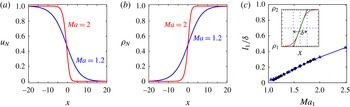
in (3.2) non-zero) for a molecular gas as described in § 4.1 (see figure 1
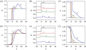
c). To further verify the present results, we have also implemented another scheme (Delis & Katsaounis Reference Delis and Katsaounis2003) that incorporates the source terms in the relaxation scheme itself by modifying the right-hand side of (3.6) – the numerical results from the two schemes agree well, see figure 2(d) in § 4.2. The interested reader is referred to Delis & Katsaounis (Reference Delis and Katsaounis2003) for related details on the algorithm.
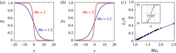
Shock-wave profiles for a molecular gas: (a) velocity and (b) density; the parameter values are
 $Ma_{1}=1.2$
(blue line) and
 $2.0$
(red line). The temperature profile (not shown) looks similar to the density profile. (c) Variation of the inverse shock width,
 $l_{1}/{\it\delta}$
, with
 $Ma_{1}$
. The triangles show the present solution of the NS equations and the circles show the NS solution of Torrilhon & Struchtrup (Reference Torrilhon and Struchtrup2004). The inset in (c) illustrates the definition of the shock width
 ${\it\delta}$
.
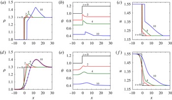
Predictions of the Euler model (a–c) and the Navier–Stokes model (d–f) for shock profiles of (a,d) density, (b,e) granular temperature and (c,f) velocity at different times (
 $t=0,2,4,10$
) for
 $Ma_{1}=1.2$
and
 ${\it\alpha}=0.9$
. The circles in (d) represent the density profile at
 $t=10$
obtained from a different numerical scheme (see the text in the last paragraph in § 3.2).
4. Results and discussion: granular versus molecular shock waves
4.1. Shock waves in a molecular gas and validation of the numerical scheme
Here, we consider normal shock waves propagating in a molecular gas (i.e. the restitution coefficient is
 ${\it\alpha}=1$
, see § 2) and validate the present numerical scheme. The upstream boundary conditions are taken as
 $$\begin{eqnarray}{\it\rho}_{1}=1,\quad u_{1}=Ma_{1}\sqrt{{\it\gamma}},\quad {\it\theta}_{1}=1,\end{eqnarray}$$
where
 $Ma_{1}$
is the upstream Mach number (2.20), while the downstream boundary conditions are provided by the RH conditions (2.21). The initial discontinuity is placed at
 $x=0$
and the numerical experiments are carried out over a domain of length
 $L=50$
covering
 $(-L/2,L/2)$
with
 $2000$
grid points, with a time step of
 ${\rm\Delta}t=(\mathscr{C}{\rm\Delta}x/\text{max}\,a_{i})$
. For all calculations we set the CFL number to
 $\mathscr{C}=0.01$
; the relaxation rate in (3.6) is set to
 ${\it\epsilon}=10^{-8}$
as this provides converged results. The computations are carried out over a long time (
 $t>100$
) such that the hydrodynamic profiles attain a time-invariant state as expected for shocks propagating in an ideal gas.
The velocity and density profiles, predicted by the Navier–Stokes model, are displayed in figure 1(a,b); it should be noted that the profiles have been normalized such that
 $u_{N}=(u-u_{2})/(u_{1}-u_{2})$
and
 ${\it\rho}_{N}=({\it\rho}-{\it\rho}_{1})/({\it\rho}_{2}-{\it\rho}_{1})$
. In each panel, the blue and red lines represent data for upstream Mach numbers of
 $Ma_{1}=1.2$
and
 $2$
respectively. It is seen that there are strong gradients across the ‘shock layer’ for each hydrodynamic field, and the width/thickness of this layer decreases with increasing
 $Ma_{1}$
.
As in previous works (Gilbarg & Paolucci Reference Gilbarg and Paolucci1953; Torrilhon & Struchtrup Reference Torrilhon and Struchtrup2004), a characteristic width of the density profile is chosen to define the ‘thickness’ of the shock:
 $$\begin{eqnarray}{\it\delta}=({\it\rho}_{2}-{\it\rho}_{1})/\max (\partial {\it\rho}/\partial x),\end{eqnarray}$$
which is schematically depicted in the inset of figure 1(c). The variation of the inverse of the shock thickness (
 $l_{1}/{\it\delta}$
) with upstream Mach number (
 $Ma_{1}$
) is shown in the main panel of figure 1(c); the solutions of the present numerical scheme are denoted by blue triangles which almost overlap with black circles which represent data of Torrilhon & Struchtrup (Reference Torrilhon and Struchtrup2004) using a different numerical scheme. On the whole, figure 1(c) confirms the accuracy of our numerical scheme.
4.2. Shock structures in a granular gas and Haff’s law
For shocks in a granular gas, all computations were carried out in a larger domain of length
 $4000$
covering
 $(-2000,2000)$
with a varying number of grid points; a spatial step size of
 ${\rm\Delta}x=0.05$
was found to be sufficient for the early time evolution of the shock, but the results at late times (figure 6) were obtained with
 ${\rm\Delta}x=0.01$
. Results are presented as functions of the restitution coefficient (
 ${\it\alpha}$
) and the ‘initial’ upstream Mach number
 $Ma_{1}=u_{1}/\sqrt{{\it\gamma}{\it\theta}_{1}(t=0)}$
, see (2.20), where
 ${\it\theta}_{1}(t=0)$
is the initial upstream temperature. In the following, the ‘granular’ shock is defined as a layer over which all hydrodynamic quantities undergo changes from upstream to downstream values.
The early time dynamics (up to
 $t=10$
) of the density
 ${\it\rho}(x,t)$
, the granular temperature
 ${\it\theta}(x,t)$
and the gas velocity
 $u(x,t)$
are shown in figure 2 for
 $Ma_{1}=1.2$
and
 ${\it\alpha}=0.9$
. The profiles obtained from the Euler and Navier–Stokes models are contrasted in panels (a–c) and (d–f) respectively. It is seen that while the initial discontinuity of the hydrodynamic fields seems to persist at all times for the Euler model, all profiles become smoother with time due to the diffusive action of viscosity for the NS model. We observe that the density profile (a,d) develops an ‘overshoot’ within the shock in the sense that the maximum density (
 ${\it\rho}_{max}$
) is larger than its downstream value and this overshoot (
 $={\it\rho}_{max}-{\it\rho}_{2}$
) increases as time progresses; this will be discussed in detail in § 4.2.1. Panels (b,e) indicate that both the upstream and downstream temperatures decay with time, and the maximum temperature (
 ${\it\theta}_{max}$
) occurs within the shock layer; this will be discussed in detail in § 4.2.2. The velocity profiles in (c,f) indicate that the local Mach number is maximum in the upstream state and decreases through the shock, reaching its minimum value in the downstream state. The qualitative nature of the hydrodynamic profiles at higher
 $Ma_{1}$
remains similar to that in figure 2, and is not shown for the sake of brevity.
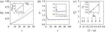
(a) Temporal evolution of the density overshoot,
 ${\rm\Delta}{\it\rho}\equiv ({\it\rho}_{max}-{\it\rho}_{2})$
, for
 $Ma_{1}=1.2$
and
 ${\it\alpha}=0.9$
. The inset shows the variation of the spatial location of
 ${\it\rho}_{max}$
with time. (b) Evolution of the normalized shock speed,
 $\tilde{v}_{s}=v_{s}/c$
, where
 $v_{s}=x({\it\rho}={\it\rho}_{max})/t$
is the speed of the density peak and
 $c=\sqrt{{\it\gamma}{\it\theta}_{1}}$
is the adiabatic sound speed, for
 $Ma_{1}=1.2$
(main panel) and
 $Ma_{1}=2$
(inset), with
 ${\it\alpha}=0.9$
. (c) Variation of the asymptotic shock speed
 $\tilde{v}_{s}^{\infty }$
(extracted from the numerical solution of the granular Navier–Stokes equations, dubbed ‘NS solution’) with
 $Ma_{1}$
(inset) and inelasticity (main panel):
 $Ma=1.2$
▴;
 $Ma=1.5$
▪;
 $Ma=2.0$
♦;
 $Ma=3.0$
●.
4.2.1. Density overshoot and its propagation speed
The time evolution of the density overshoot,
 ${\rm\Delta}{\it\rho}\equiv ({\it\rho}_{max}-{\it\rho}_{2})$
, for an upstream Mach number of
 $Ma_{1}=1.2$
and a restitution coefficient of
 ${\it\alpha}=0.9$
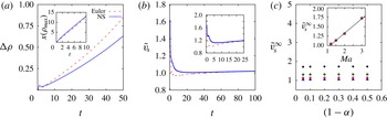
is shown in figure 3(a) – the red dashed and blue solid lines denote the predictions of the Euler and NS models respectively. While
 ${\rm\Delta}{\it\rho}=0$
for a molecular gas (figure 1
b and Gilbarg & Paolucci Reference Gilbarg and Paolucci1953; Torrilhon & Struchtrup Reference Torrilhon and Struchtrup2004), we find that
 ${\rm\Delta}{\it\rho}>0$
in a granular gas, and its magnitude increases with time; it should be noted that
 $({\rm\Delta}{\it\rho})_{NS}<({\rm\Delta}{\it\rho})_{Euler}$
, except for very short early times. We also found (not shown) that
 ${\rm\Delta}{\it\rho}$
increases with increase in the Mach number and/or the dissipation. The occurrence of density overshoot is a novel feature of ‘granular’ shock waves, and its large-time behaviour is discussed in § 4.2.3.
The inset of figure 3(a) indicates that the spatial position of
 ${\it\rho}_{max}$
shifts to the right with time, from which a shock speed can be estimated. The speed of propagation of the density maximum is defined as
 $v_{s}=x({\it\rho}={\it\rho}_{max})/t$
, and its temporal variations for
 $Ma_{1}=1.2$
and
 $2$
are displayed in the main panel and the inset of figure 3(b) respectively, with
 ${\it\alpha}=0.9$
. It is seen that the normalized shock speed,
 $\tilde{v}_{s}=v_{s}/c$
(where c is the adiabatic sound speed, (2.20)), reaches a steady asymptotic value at large times for both the Euler (red curve) and the NS (blue curve) models. Comparing the inset with the main panel, we find that
 $\tilde{v}_{s}^{\infty }\equiv \tilde{v}_{s}(t\rightarrow \infty )$
is higher at higher
 $Ma_{1}$
. This is further evident from figure 3(c), which shows the variation of
 $\tilde{v}_{s}^{\infty }$
with
 $(1-{\it\alpha})$
for a range of
 $Ma_{1}$
. While
 $\tilde{v}_{s}^{\infty }$
does not depend on the restitution coefficient, it increases linearly with increasing
 $Ma_{1}$
(see the inset of 3
c). Overall, we may conclude from figure 3(b,c) that the density peak travels with a steady constant speed at sufficiently late times; this conclusion is similar to that found for a piston-driven shock wave (Kamenetsky et al.
Reference Kamenetsky, Goldshtein, Shapiro and Degani2000).
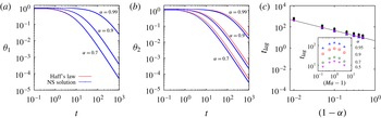
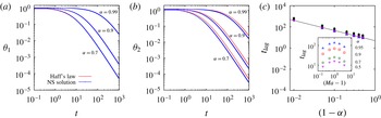
(a,b) Comparison of Haff’s law (red curve) with the numerical solution of the NS equations for
 $Ma_{1}=1.2$
: (a) upstream temperature
 ${\it\theta}_{1}$
and (b) downstream temperature
 ${\it\theta}_{2}$
. (c) Dependence of the time lag (
 $t_{lag}$
, between the downstream temperature
 ${\it\theta}_{2}$
and that obtained from Haff’s law) on the inelasticity (main panel) and
 $Ma_{1}$
(inset); see the text for the definition of
 $t_{lag}$
:
 $Ma=1.2$
▴;
 $Ma=1.5$
▪;
 $Ma=2.0$
♦;
 $Ma=3.0$
●;
 $Ma=5.0$
▾.
4.2.2. Temperature profiles: Haff’s law and scaling relations
For an undriven granular gas with initial temperature
 ${\it\theta}(0)$
, the hydrodynamic equations admit a spatially homogeneous solution (
 $\boldsymbol{{\rm\nabla}}({\it\rho},\boldsymbol{u},{\it\theta})=0$
) with a time-dependent temperature (
 ${\it\theta}(x,t)\equiv {\it\theta}(t)$
) such that the gas cools according to Haff’s law (Haff Reference Haff1983):
 $$\begin{eqnarray}{\it\theta}(t)=\frac{{\it\theta}(0)}{(1+t/{\it\tau}_{H})^{2}},\quad \text{where }{\it\tau}_{H}=\frac{3}{2nd^{2}\sqrt{{\rm\pi}}(1-{\it\alpha}^{2})(1+3a_{2}/16)}\end{eqnarray}$$
is the relaxation time. Equation (4.3) represents the well-known ‘homogeneous cooling state’ (HCS) of a granular gas. A departure from (4.3) occurs when the system becomes inhomogeneous with cluster formation, called the ‘inhomogeneous cooling state’ (ICS, Luding & Herrmann Reference Luding and Herrmann1999). From here onwards, all results are presented for the Navier–Stokes model of a granular gas.
We recall from figure 2(b,e) that the temperatures at the upstream (
 ${\it\theta}_{1}\equiv {\it\theta}(x=-L/2)$
) and downstream (
 ${\it\theta}_{1}\equiv {\it\theta}(x=L/2)$
) ends decay as time progresses. The temporal evolutions of
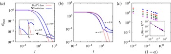
 ${\it\theta}_{1}$
and
 ${\it\theta}_{2}$
are compared with (4.3) in figure 4(a,b) respectively. It is clear that the upstream temperature closely follows Haff’s law for all
 ${\it\alpha}$
; however, the downstream temperature lags (4.3) in time. We calculate this time lag, defined via
 $t_{lag}=[t_{Haff}(\tilde{{\it\theta}}_{2}=0.01)-t_{NS}(\tilde{{\it\theta}}_{2}=0.01)]$
, such that
 $\tilde{{\it\theta}}_{2}\equiv {\it\theta}_{2}(t)/{\it\theta}_{2}(0)=0.01$
. It is seen from figure 4(c) that
 $t_{lag}$
decreases with increasing dissipation,
 $t_{lag}\sim (1-{\it\alpha})^{-19/20}$
, but follows a non-monotonic variation with the upstream Mach number
 $Ma_{1}$
. We speculate that the ‘finite’ shock speed might be responsible for the earlier decay of downstream temperature compared with that dictated by Haff’s law.
(a) Temporal evolution of the maximum granular temperature
 ${\it\theta}_{max}$
for
 $Ma_{1}=1.2$
; Haff’s law is denoted by the red curve and the blue curves represent numerical solutions for
 ${\it\alpha}=0.9$
and
 $0.7$
; the inset shows a zoomed part of the same figure (see text). (b) The same as (a) but for
 $Ma_{1}=2$
. (c) Variation of the critical time
 $t_{c}$
(at which the numerical solution
 ${\it\theta}_{max}$
crosses/overtakes Haff’s solution) with
 $(1-{\it\alpha})$
for different values of
 $Ma_{1}$
; the inset shows the scaling (4.4) for data collapse, see the text:
 $Ma=1.2$
▴;
 $Ma=1.5$
▪;
 $Ma=2.0$
♦;
 $Ma=3.0$
●;
 $Ma=5.0$
▾.
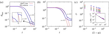
The time evolution of the maximum granular temperature (
 ${\it\theta}_{max}$
) is shown in figure 5(a,b) for
 $Ma_{1}=1.2$
and
 $2$
respectively, with
 ${\it\alpha}=0.9$
(upper curve) and
 $0.7$
(lower curve); Haff’s solution, denoted by the red line, is also superimposed for each value of
 ${\it\alpha}$
. For the case of a weak shock (
 $M=1.2$
),
 ${\it\theta}_{max}$
seems to follow Haff’s law up to a critical time (marked by the vertical black line in the inset of figure 5
a for
 ${\it\alpha}=0.9$
), but decays much slower thereafter. For a strong shock (
 $M=2$
), however,
 ${\it\theta}_{max}$
decays at a faster rate than Haff’s law for
 $t<t_{c}$
and at a slower rate for
 $t>t_{c}$
. The gradients of the hydrodynamic fields in the shock layer (see figure 2) might be responsible for the faster decay of
 ${\it\theta}_{max}$
at early times. On the other hand, the departure of
 ${\it\theta}_{max}$
from Haff’s law beyond
 $t>t_{c}$
, leading to a near-saturation of
 ${\it\theta}_{max}$
at large times (see the blue curves for
 $t>200$
in figure 5
b), is reminiscent of the temperature evolution in the inhomogeneous cooling state (Pöschel & Luding Reference Pöschel and Luding2001). (The weak and strong shocks correspond to Mach numbers of
 $Ma\sim 1$
and
 $Ma\gg 1$
respectively. In the present work, we followed Grad’s moment theory (Torrilhon & Struchtrup Reference Torrilhon and Struchtrup2004), which gives a critical Mach number of
 $Ma_{cr}\approx 1.65$
above which the 13-moment equations do not admit continuous solutions.)
The critical time (
 $t_{c}$
) at which the shock solution
 ${\it\theta}_{max}$
crosses/overtakes Haff’s solution (see figure 5
a,b) decreases with increasing inelasticity
 $(1-{\it\alpha})$
and upstream Mach number
 $Ma_{1}$
, as is evident from the main panel of figure 5(c). Interestingly, the data for all
 $Ma_{1}$
can be collapsed via the following scaling relation:
 $$\begin{eqnarray}t_{c}\sim (Ma_{1}-1)^{-9/8}(1-{\it\alpha})^{-17/20},\end{eqnarray}$$
denoted by the black line in the inset of figure 5(c). The exponents in (4.4) have been determined via a least-square fitting of all data, with a standard deviation of less than 2 %.
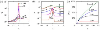
Temporal evolution of (a) density and (b) pressure for
 $Ma_{1}=2$
and
 ${\it\alpha}=0.7$
. (c) Arrest of the maximum density
 ${\it\rho}_{max}$
via a regularization procedure (see the text in § 4.2.3 for details).
4.2.3. Large-time behaviour: density overshoot, pressure instability and regularization
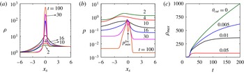
Lastly, we address the issue of the large-time behaviour of granular shock profiles. Figure 6(a,b) displays the density and pressure profiles at different times for parameter values of
 $Ma_{1}=2$
and
 ${\it\alpha}=0.7$
. In both panels, the abscissa,
 $x_{s}=x-x({\it\rho}_{max})$
, has been scaled with respect to the location of the maximum density
 ${\it\rho}_{max}$
. For this parameter set, the location of the density maximum (panel a) is found to coincide with that of a local pressure minimum
 $p_{min}^{loc}$
(panel b) for
 $t\geqslant 16$
(which also coincides with a local minimum of the granular temperature
 ${\it\theta}_{min}\equiv {\it\theta}({\it\rho}={\it\rho}_{max})$
, not shown). These overall findings also hold for other parameter values of
 $Ma_{1}$
and
 ${\it\alpha}$
. The higher pressures on both sides of
 ${\it\rho}_{max}$
create pressure differences that drive the particles to rush in from both sides, thereby enhancing
 ${\it\rho}_{max}$
with time (see the green line in c). This mechanism is akin to the well-known pressure instability which drives cluster formation due to collisional cooling in both (i) undriven (Goldhirsch & Zanetti Reference Goldhirsch and Zanetti1993) and (ii) driven (Alam & Nott Reference Alam and Nott1998; Gayen & Alam Reference Gayen and Alam2006; Alam, Shukla & Luding Reference Alam, Shukla and Luding2008) granular gases.
Figure 6(c) confirms that
 ${\it\rho}_{max}$
keeps increasing with time, and hence the density profile
 ${\it\rho}(x,t)$
would keep changing as
 $t\rightarrow \infty$
. This points towards an apparent deficiency of the inelastic hard-sphere model, and some important physics is missing in it: within the denser/clustered region, the impact velocities are probably lower compared with those in the dilute homogeneous region, and hence the collisional dissipation would be lower in the denser regions. The latter point can be justified by recalling the fact that the restitution coefficient (of real particles) approaches its elastic limit (
 ${\it\alpha}\rightarrow 1$
) as the impact velocity decreases (Goldhirsch Reference Goldhirsch2003). This can be incorporated in the present model by rewriting the collisional dissipation rate as
 $$\begin{eqnarray}\mathscr{D}_{reg}=\mathscr{F}({\it\xi})\mathscr{D}\equiv (1+{\it\xi}^{2})\exp (-{\it\xi}^{2})\mathscr{D},\end{eqnarray}$$
where the ‘regularization’ factor
 $\mathscr{F}({\it\xi})$
has been exactly evaluated in Luding & Goldshtein (Reference Luding and Goldshtein2002), to which the reader is referred for related details on the collision model with a ‘cutoff’ restitution coefficient. In (4.5),
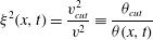 $$\begin{eqnarray}{\it\xi}^{2}(x,t)=\frac{v_{cut}^{2}}{v^{2}}\equiv \frac{{\it\theta}_{cut}}{{\it\theta}(x,t)}\end{eqnarray}$$
is identified with the ratio between a critical/cutoff impact energy
 ${\it\theta}_{cut}$
and the local fluctuation energy (granular temperature). It is clear that
 $\mathscr{D}_{reg}=\mathscr{D}$
for
 ${\it\xi}^{2}=0={\it\theta}_{cut}$
, recovering the original constitutive model of § 2, and
 $\mathscr{D}_{reg}<\mathscr{D}$
for
 ${\it\xi}^{2}>0$
. Lastly, we set
 $\mathscr{D}_{reg}=0$
whenever
 $\mathscr{F}({\it\xi}(x,t))<\mathscr{F}_{cr}\ll 1$
; as an illustration we have used
 $\mathscr{F}_{cr}=0.05$
, which translates into a critical value of
 ${\it\xi}_{cr}^{2}\approx 4.75$
(and hence
 ${\it\theta}_{min}\approx 0.21{\it\theta}_{cut}$
) below which the particle collisions are treated as elastic.
With the dissipation rate being given by (4.5) and assuming that other transport coefficients (
 ${\it\mu}$
,
 $p$
,
 ${\it\kappa}$
and
 ${\it\kappa}_{h}$
) remain unaffected, we have solved (2.13)–(2.15) for the same shock-wave problem by specifying different values of
 ${\it\theta}_{cut}$
. As a proof of concept, the results are shown in figure 6(c), which confirms that the continual increase of
 ${\it\rho}_{max}$
can indeed be arrested, see the black and red lines for
 ${\it\theta}_{cut}=0.01$
and
 $0.05$
respectively. The smaller the value of
 ${\it\theta}_{cut}$
is, the larger the time to reach the arrested state of
 ${\it\rho}_{max}$
is. For a ‘dense’ granular gas, the arrested maximum density can be tied with the random-packing limit, suggesting a ‘gas–solid’ transition, as in the work of Kamenetsky et al. (Reference Kamenetsky, Goldshtein, Shapiro and Degani2000) for piston-driven granular shock waves. The same transition can also be addressed within the present regularized model (4.5) by employing the transport coefficients for a dense granular gas. A detailed investigation of these issues is relegated to a future work.
5. Conclusions
The Riemann problem of granular shock waves was analysed by numerically solving the granular hydrodynamic equations. The density and temperature profiles were found to be asymmetric, with the maxima of both density and temperature occurring within the shock layer, which constitute two distinguishing features of the ‘granular’ Riemann problem (compared with that for ideal gases). The fundamental difference of the granular shock problem from its ideal-gas counterpart can be tied to ‘inelastic dissipation’, since this makes the upstream and downstream states of a granular shock live in non-equilibrium ‘decaying’ states (similar to HCS), which, in turn, is responsible for the non-trivial shock structures uncovered here. Inside the shock too, Haff’s law was found to hold for the maximum temperature, but for weak shocks (
 $Ma_{1}\sim 1$
) only, and deviations occurred for strong shocks. A scaling relation (4.4) was uncovered which expresses the critical time (at which the maximum temperature deviates from Haff’s law) as a function of the Mach number and inelasticity. The origin of asymmetric density profiles, leading to the continual build-up of density inside the shock, seems to be tied to a pressure instability in granular gases. A simple regularization procedure to arrest the maximum density has been proposed. Future work on shock waves should employ the ‘regularized’ version of the granular hydrodynamic equations.
Acknowledgement
We thank Dr S. Ansumali for discussions on the numerical scheme.