





1 Introduction
Mean or sum scores are commonly used in psychometric scales to summarize responses to multi-item instruments in psychology and related fields, especially when items are ordinally scaled (Sijtsma & van der Ark, Reference Sijtsma and van der Ark2020, see, e.g., p. 9, and Chapters 2 and 3). In a recent retrospective paper, Sijtsma et al. (Reference Sijtsma, Ellis and Borsboom2024) argue that the sum score is “psychometrics’ greatest accomplishment.” Suppose a respondent takes a psychometric test with items
$X_1,\ldots ,X_J$
 . We take a latent variable perspective and assume that there is a latent variable
$\theta $
 influencing the items, which is often interpreted as latent ability. Then

are the respondent’s mean and true scores. In this article, we study the relations among
$\bar X_J$
 ,
$T_J(\theta )$
 , and
$\theta $
 under weak conditions, and in the process formulate a new model class called martingale factor models. We then study the increasing-item convergence of the mean score and the true score, and illustrate psychometrically relevant consequences of this convergence.
To frame our investigation, consider the following standard assumption set for nonparametric IRT (see, e.g., Mokken & Lewis, Reference Mokken and Lewis1982).
Assumption 1.
-
(1)
-
(a) For each $j=1,\ldots ,J$
 ,
$X_j\in \{0,1,\ldots ,K\}$
.
-
(b) There is a random variable $\theta $
such that
$X_1,\ldots ,X_J$
are conditionally independent given
$\theta $
.
-
-
(2) The random variable $\theta $
is univariate. -
(3) For each $j=1,\ldots ,J$
and each
$k=0,\ldots ,K$
, the function
$\theta \mapsto P_\theta (X_j>k)$
is non-decreasing in
$\theta $
, where
$P_\theta (\cdot )=P(\cdot | \theta )$
.


Under Assumption 1, the mean score is close to the true score, and we explain why this is so in Section 2.1. Indeed, the upcoming Proposition 3(1) shows that for any
$\lambda> 0$
 ,

Further, Assumption 1(2) and (3) imply that
$ T_J(\theta ) =J^{-1} \sum _{j=1}^J \sum _{k=0}^{K-1} P_\theta (X_j>k) $
 is non-decreasing in
$\theta $
 . Therefore, the mean score concentrates around a non-decreasing transformation of
$\theta $
 , hence motivating its wide use in empirical practice.
This raises two natural questions. First, under what conditions is the observed mean score a good approximation to the true score? Second, under what conditions is the true score, for large J, no longer sensitive to the removal of a vanishingly small fraction of items? The first question concerns within-form approximation: whether the operational score tracks the true score of the administered item sequence. The second can be understood as between-form stability: whether the true scores of large item sets with slightly different items become mutually close. When both properties hold, the mean score converges to a stable function of the latent variable.
The psychometric importance of question (i) is well-established (see, e.g., Junker, Reference Junker1991; Stout, Reference Stout1990) and is studied in Section 2. Assumption 1(1)(b) is (Kallenberg, Reference Kallenberg2021, Theorem 8.12, the chain rule of conditional independence) equivalent to saying that, for each
$j=1,\ldots ,J$
 ,

We will show that foundational large-J results continue to hold under the weaker requirement
$ E(X_j | X_1, X_2, \ldots , X_{j-1}, \theta ) = E ( X_j | \theta ), $
 which, together with item integrability, defines the martingale factor model in
$\theta $
 (Section 2.2). For binary items, success probabilities and expectations coincide, meaning that the two model classes then coincide, as shown below. But for polytomous items, the martingale factor model assumption is considerably weaker than conditional independence, as it imposes only a conditional mean restriction rather than a full conditional distributional statement. Conditional expectations are the best least-squares predictors, and the practical interpretation of a martingale factor model is that once you know a person’s ability, you cannot usefully use previously answered items to gain additional predictive power for the next item’s outcome. Also, we show in Section 2.2 that items
$(X_1, X_2, \ldots )$
 fulfill Assumption 1(1)(b) if and only if
$(f(X_1), f(X_2), \ldots )$
 is a martingale factor model in
$\theta $
 for any bounded measurable function f, which means that the martingale factor model can be seen as more foundational than conditional independence.
Question (ii) is connected to domain-sampling perspectives and generalizability theory in psychometrics and concerns whether form-specific true scores stabilize as the item set grows. In Section 3, we study this large-J stability and show it to be equivalent to the convergence of
$T_J(\theta )$
 to a random variable
$T(\theta )$
 depending only on
$\theta $
 . Random item pools provide one natural psychometric mechanism by which such a convergence takes place, and we identify other possible mechanisms by which it may occur. Let
$o_P(1)$
 denote a quantity converging to zero in probability as
$J \to \infty $
 . When the true score converges and
$\bar X_J = T_J(\theta ) + o_P(1)$
 holds, we obtain
$ \bar X_J = T(\theta ) + o_P(1), $
 which in Definition 5 we call convergent estimability. When convergent estimability can be justified (through substantive means), the analysis of a range of psychometrically relevant problems simplifies, and we illustrate this in a few substantive examples.
The article has two core theoretical contributions. First, Section 2.2 shows that Assumption 1(1)(b) can be weakened to the martingale factor model assumption while still yielding a tractable inference framework for mean scores based on martingale methods. Second, Section 3 shows that, under standard assumptions together with a between-form stability condition, the mean score admits the same large-J interpretation as under an infinite-item-pool perspective. The remaining parts of the article develop consequences and illustrations of this theory.
The structure of the article is as follows. In Section 2, we turn to question (i), namely, when and why mean scores approximate true scores under assumptions weaker than conditional independence. We then introduce martingale factor models and show that conditionally independent items are martingale factor models. For bounded items, we show that martingale factor models imply non-asymptotic exponential concentration of
$\bar X_J$
 around
$T_J(\theta )$
 as in (1), as well as asymptotic normality of weighted mean scores. We show that a certain mixture of martingale factor models is again a martingale factor model, and that conditional independence can be described through martingale factor model assumptions on transformed items. Some non-trivial examples of martingale factor models are given in Appendix D of the Supplementary Material. Section 3 turns to question (ii). We identify criteria under which
$T_J(\theta )$
 converges and show that if
$E (X_j|\theta )$
 is parameterized by a sequence of numbers that have a long-run stability property that we call the law of large numbers property, the true score converges.
In Section 4, we turn to theoretical consequences and illustrations of the results in Sections 2 and 3. We derive unconditional and person-specific confidence intervals for the true score based on a martingale factor model item sequence for a single respondent and consider some immediate consequences for ranking ability. We then consider some consequences of convergent estimability and study mean-score correlations and nonparametric factor scores (NPFSs) based on a quantile matching strategy. The theoretical applications are illustrated numerically in Section 5.
First, Section 5.1 considers a simple threshold model, and analytically derives the limiting behavior of mean-score correlations, which are then confirmed numerically. Section 5.2 calculates the limiting bias of an asymptotic confidence interval for a threshold model, and Section 5.3 studies the confidence intervals we consider more systematically, with supplementary simulations under local dependence in Appendix D.1 of the Supplementary Material. Section 5.4 then compares mean-score correlations, correlations between NPFSs, and model-based correlation estimates. While standard parametric models are superior to both mean-score correlations and correlations among NPFSs when the parametric model conditions are exactly fulfilled, Section 5.4 shows that this may be reversed when the parametric model is misspecified.
While these numerical examples are non-trivial, they do not aim at maximum generality, but are meant to complement and verify the theoretical illustrations of Sections 2 and 3.
Earlier work on mean scores often makes parametric assumptions, as in Choe and Han (Reference Choe and Han2022), Guo and Dorans (Reference Guo and Dorans2020), Kim (Reference Kim2013), and Kolen et al. (Reference Kolen, Zeng and Hanson1996). Since our assumptions are nonparametric, our analysis also covers cases where standard parametric models are misspecified. This is precisely a setting where mean scores may outperform more elaborate parametric methods in empirical work, as illustrated by a mean-score correlation simulation reported in Section 5.4. While this illustration is in favor of using mean-score correlations, our theoretical analysis shows that mean-score correlations are in all but exceptional circumstances inconsistent for the latent correlation, and instead estimate the correlation between functions of the latent variables. Except under strong conditions, these functions are not identified from the distribution of the items. When reasonable parametric models are known, they should be preferred in empirical applications.
Practitioners often use mean scores without explicit commitment to an underlying latent-variable model, and this practice can be justified through other means that we do not consider in the present article. Our analysis is not intended as a direct foundation for all uses of sum scores in practice, but shows what can be said about mean scores within an IRT-type latent-variable framework when one is unwilling to impose strong parametric assumptions.
Except when otherwise stated, our analysis is compatible with both ordinal and continuous data. In the ordinal case, item responses take values in the set
$\{0, 1, \ldots , K\}$
 , while, in general, we sometimes assume the item responses to be contained in an interval of length K.
The article also has clear limitations. Although our assumptions are weak in distributional terms, the analysis relies on increasing-item asymptotics and mostly assumes the absence of planned or unplanned missing observations. Further, the confidence intervals and NPFSs we suggest ought to be studied under a greater variety of conditions before they are considered as finished methodological tools.
All proofs are found in the Supplementary Material. All references to an appendix are to sections in the Supplementary Material. A map of the results of the article is provided in Appendix A of the Supplementary Material, and a table of the notation is given in Appendix B of the Supplementary Material. Stochastic order symbols and limits are with respect to
$J\xrightarrow {}\infty $
 unless otherwise stated. The convergence arrows
$\xrightarrow {D}$
 ,
$\xrightarrow {P}$
 , and
$\xrightarrow {}$
 denote convergence in distribution, convergence in probability, and ordinary convergence, respectively. Each section in the numerical illustration section has a separate reproducibility script in R (R Core Team, 2020), available at https://osf.io/s5gwx.
2 Mean scores as approximate true scores: General results and martingale factor models
We now consider when and why mean scores approximate true scores under weaker assumptions than Assumption 1. We start by extending some foundational results and definitions of Stout (Reference Stout1990) and Junker (Reference Junker1991) concerning essential independence and related convergence concepts. Based on this analysis, we propose a new model class that we call martingale factor models. This class generalizes nonparametric item response models under Assumption 1, but replaces the assumption of conditional independence with a martingale-type assumption. We show that in this model class, mean scores are exponentially concentrated around true scores, and that centered mean scores, standardized by their conditional standard deviations, are conditionally and unconditionally asymptotically normal under weak conditions.
2.1 Definitions of convergence of mean scores
Here, we explain why mean scores approximate true scores under Assumption 1 and consider this convergence under weaker assumptions than Assumption 1. We assume that
$\theta $
 is a random vector of finite dimension, which allows us to deal with conditional probabilities as though they were standard probability measures (Shiryaev, Reference Shiryaev1996, Theorems 4 and 5, Chapter II.7), as considered in more detail below as needed. We start by recalling the technical definition of the conditional independence made in Assumption 1(1)(b).
Definition 1. We say that
$X = (X_1, X_2, \ldots )$
 is conditionally independent given a random vector or variable
$\theta $
 if for any
$J \geq 1$
 and any numbers
$x_1, x_2, \ldots , x_{J}$
 , we have
$ P(X_1 \leq x_{1}, \ldots , X_{J} \leq x_{J} | \theta ) = \prod _{j=1}^{J} F_{j|\theta }(x_j), $
 where
$F_{j|\theta }(x_j) = P(X_j \leq x_{j} | \theta )$
 .
Remark 1. There will be an equivalence class of latent variables
$\theta $
 which fulfills this requirement. For example, if X is conditionally independent given
$\theta $
 , it is also the case that X is conditionally independent given
$\tilde \theta = S(\theta )$
 whenever
$\sigma (\tilde \theta )=\sigma (\theta )$
 ; for example, this holds when S is a measurable bijection with measurable inverse. Results for conditionally independent variables will therefore hold simultaneously for all compatible latent variables. This is true even under strong assumptions on the items, see, for example, Grønneberg and Foldnes (Reference Grønneberg and Foldnes2019) for an illustration of this phenomenon for threshold models, where simulating from the Vale and Maurelli (Reference Vale and Maurelli1983) method and then discretizing these observations into ordinal observations may be observationally equivalent to discretizing exactly normal observations. Except for results that apply directly to
$\theta $
 , such as the later result on consistent estimates of
$\theta $
 , our results apply to an equivalence class of latent variables and not to a single, identified
$\theta $
 .
We have the following useful representation for conditionally independent variables. While the representation is a consequence of abstract representation results found, for example, in Kallenberg (Reference Kallenberg2021, Chapter 8), an elementary proof is provided for completeness. As in standard stochastic representations, we assume that the probability space is sufficiently rich to support a sequence
$U_1,U_2,\ldots $
 of independent and identically distributed uniform random variables on
$[0,1]$
 that are independent of
$\theta $
 . This can be achieved by possibly expanding the probability space (see Kallenberg, Reference Kallenberg2021, p. 176) and is therefore assumed essentially without loss of generality. For a cumulative distribution function F, let
$F^{-1}(x) = \inf \{ t: F(t) \geq x \}$
 be its generalized inverse.
Lemma 1. Suppose
$X_1, X_2, \ldots $
 are conditionally independent given
$\theta $
 . Then the distribution of
$(X_1, X_2, \ldots )'$
 is the same as if

where
$U_1,U_2, \ldots $
 are each uniform on
$[0,1]$
 and are independent of each other and of
$\theta $
 .
By slight abuse of notation, we will sometimes write
$X_j = F_{j|\theta }^{-1}(U_j)$
 , as all results in this article concern properties of distributions. For conditionally independent items,
$J^{-1} \sum _{j=1}^{J} X_j = J^{-1} \sum _{j=1}^{J} F_{j|\theta }^{-1}(U_j)$
 which for fixed
$\theta $
 will be close to the average of
$E [F_{j|\theta }^{-1}(U_j) ]_U$
 by the law of large numbers for independent variables, where
$E[\cdot ]_U$
 means integration with respect to
$(U)$
 only. The independence between
$(U)$
 and
$\theta $
 implies
$E [F_{j|\theta }^{-1}(U_j) ]_U = E [ X_j | \theta ]$
 , and we therefore expect

to converge to zero. This convergence, in the sense of the upcoming Definition 2(2), defines consistent estimability, similar to Stout (Reference Stout1990) and Junker (Reference Junker1991).
Remark 2. As in Junker (Reference Junker1991), we do not consider the sub-test-perspective of Stout (Reference Stout1990, Definition 3.2 and Equation (Reference Grønneberg, Moss and Foldnes19)) related to his analysis of test dimensions. The following definitions can be asked to hold for each non-sparse sub-test (see Stout, Reference Stout1990, Equation (4)). We do not consider this further.
Recall that an essential supremum with respect to a distribution say
$F_\theta $
 , is one that is taken up to
$F_\theta $
 -null sets, where
$F_\theta $
 is here the distribution of
$\theta $
 . Fixed values of
$\theta $
 are denoted by
$\vartheta $
 . When pointwise notation such as
$P_\vartheta $
 ,
$E_\vartheta $
 ,
$\text {Var}\,_\vartheta $
 , and
$\mathrm {Cov}_\vartheta $
 is used, it refers to a fixed regular conditional probability kernel
$\vartheta \mapsto P_\vartheta :=P(\,\cdot \,|\theta =\vartheta )$
 . Thus, for a measurable function g,
$\mathrm {ess\,sup}_{\vartheta } g(\vartheta )$
 denotes the smallest
$c\in [-\infty ,\infty ]$
 such that
$g(\vartheta )\le c$
 for
$F_\theta $
 -almost every
$\vartheta $
 . As far as we can tell, (3)–(5) are new at least in the present context, although they are direct adaptations of well-known definitions to conditional probability measures.
Definition 2. Let
$\theta $
 be a random vector or variable, and let
$F_\theta $
 denote the distribution of
$\theta $
 . An item sequence is said to be:
-
(1) unconditionally consistently estimable if $\lim _{J \xrightarrow {} \infty } P (|D_{J}|> \varepsilon ) = 0$
for any
$\varepsilon> 0$
. -
(2) consistently estimable if $\lim _{J \xrightarrow {} \infty } P(|D_J|>\varepsilon |\theta ) = 0$
almost surely for any
$\varepsilon> 0$
. -
(3) uniformly consistently estimable if for a measurable version $p_{J,\varepsilon }(\vartheta ):=P(|D_J|>\varepsilon |\theta = \vartheta )$
, we have
$\lim _{J \xrightarrow {} \infty } \mathrm {ess\,sup}_{\vartheta } p_{J,\varepsilon }(\vartheta ) = 0$
, for any
$\varepsilon> 0$
, where the essential supremum is with respect to
$F_\theta $
. -
(4) strongly uniformly consistently estimable if for a measurable version $\tilde p_{J,\varepsilon }(\vartheta ):=P\big ( \sup _{k \geq J} |D_{k}|> \varepsilon | \theta = \vartheta \big )$
, we have
$\lim _{J \xrightarrow {} \infty } \mathrm {ess\,sup}_{\vartheta } \tilde p_{J,\varepsilon }(\vartheta ) = 0$
for any
$\varepsilon> 0$
, where the essential supremum is with respect to
$F_\theta $
. -
(5) consistently estimable with exponential concentration if for any $J \geq 1$
and any
$\varepsilon> 0$
, the inequality
$P( |D_{J}|> \varepsilon |\theta ) \leq c_1 \exp (-c_2 J^{c_3})$
holds almost surely, for some positive constants
$c_1, c_2, c_3$
that may depend on
$\varepsilon $
but not on the realized value of
$\theta $
.


Finally, X is said to be strongly unconditionally consistently estimable if
$D_{J} = o_{\text {a.s.}}(1)$
 .
As a direct consequence of the definitions and well-known results, the convergence concepts in Definition 2 are progressively stronger, and (4) implies that X is strongly unconditionally consistently estimable.
Proposition 1. The convergence concepts in Definition 2 are progressively stronger, meaning (5) implies (4), which implies (3), etc. Further, (4) implies that X is strongly unconditionally consistently estimable.
Adapting the terminology of Stout (Reference Stout1990) (again omitting his sub-test perspective, see Remark 2), we call a sequence of items that fulfill

essentially independent. By the same Chebyshev argument as in Stout (Reference Stout1990), binary items that are essentially independent fulfill the criteria of consistent estimability. The proof also transfers to bounded items in general.
For unconditional and uniform conditional consistency, similar simple criteria exist, which we now derive. We restrict attention to bounded items, that is, each item in X is contained within a fixed interval. For unbounded items, further moment assumptions are required.
Lemma 2. Suppose X has bounded items, meaning
$\sup _k |X_k| < c$
 with probability one for a number c.
-
(1) If $2 J^{-2}\sum _{1 \leq j < k \leq J} \mathrm {Cov}(X_j - E(X_j | \theta ), X_k - E(X_k | \theta )) \xrightarrow {} 0$
, then X is unconditionally consistently estimable. -
(2) If $\mathrm {ess\,sup}_{\vartheta } 2 J^{-2} \sum _{1 \leq j < k \leq J} \mathrm {Cov}_\vartheta (X_j, X_k) \xrightarrow {} 0$
, where the essential supremum is with respect to
$F_\theta $
, then X is uniformly consistently estimable. -
(3) The condition in (2) implies eq. (4), which in turn implies the condition in (1).


2.2 Martingale factor models
We now propose a model class we call martingale factor models in a latent variable
$\theta $
 . A main conclusion of this section is that martingale factor models (and hence conditionally independent items) with bounded items are consistently estimable with exponential concentration.
As mentioned in the introduction, martingale factor models replace conditional independence with the weaker requirement that the corresponding conditional means agree. This allows conditional dependence in other aspects of the conditional distribution, such as having the conditional variation of an item depending not only on
$\theta $
 but also on the candidate’s previous responses. At the end of this section (Proposition 5), we provide a class of examples which are martingale factor models but may have conditional dependence. Some concrete illustrations are given in Appendix D of the Supplementary Material.
Definition 3 (Martingale factor model)
Suppose
$X_1, X_2, \ldots $
 are random variables, and
$\theta $
 is a random vector. Suppose that for all
$j \geq 1,$
 we have that
$X_j$
 is integrable. Define
$\mathscr {F}_j := \sigma (\theta , X_1, \ldots , X_j)$
 for
$j \geq 1$
 and
$\mathscr {F}_0 = \sigma (\theta )$
 , where
$\sigma (\cdot )$
 denotes the sigma-algebra generated by the indicated variables. If

we say that
$X_1, X_2, \ldots $
 follow a martingale factor model in
$\theta $
 .
Conditional independence does not take into account the direction of time, see Definition 1 and Lemma 1, though it can be described sequentially, see eq. (2). In contrast, Definition 3 depends on the order of the items, and cannot be described without reference to the order of time. Since items are answered sequentially, this fits psychometric practice. The mathematics leaves the interpretation of this directionality open, and one natural interpretation is that the respondent’s mental state is influenced by having answered previous questions, see the discussion after Proposition 5.
The conditional expectations in Definition 3 are (nonparametric) least squares best predictors (e.g., Klenke, Reference Klenke2020, Corollary 8.17), so a martingale factor model says that once
$\theta $
 is known, no additional predictive power for item j is gained by knowing all earlier answers to the items. In contrast, conditional independence in
$\theta $
 means that once
$\theta $
 is known, additionally knowing all earlier items is completely uninformative for the current item, not merely at the level of its conditional mean, but for its entire conditional distribution.
Recall (e.g., Davidson, Reference Davidson1994, Chapter 15.1) that a martingale
$(X_j)$
 with respect to a filtration (i.e., an increasing sequence of sigma-algebras)
$(\mathscr {F}_j)$
 fulfills
$E(X_j|\mathscr {F}_{j-1}) = X_{j-1}$
 for all j and is integrable (meaning
$E |X_j| < \infty $
 for all j). Definition 3 is therefore a martingale-like assumption.
Remark 3. For an item
$X_j$
 , Ellis and Sijtsma (Reference Sijtsma, Ellis and Borsboom2024, Section 3.2) define its true score as
$E[X_j|\mathscr {G}]$
 for an appropriately chosen sigma-field
$\mathscr {G}$
 . Ellis and Sijtsma (Reference Sijtsma, Ellis and Borsboom2024, Section 3.2) show that this encompasses several earlier definitions of true scores in psychometrics. This motivates a generalization of martingale factor models, where we require that for a chosen sigma-field
$\mathscr {G}$
 , we have
$E ( X_j | \mathscr {G} \lor \sigma (X_1, \ldots , X_{j-1})) = E [X_j | \mathscr {G}]$
 for all
$j \geq 1$
 , where
$\mathscr {G} \lor \sigma (X_1, \ldots , X_{j-1})$
 is the smallest sigma field containing both
$\mathscr {G}$
 and
$\sigma (X_1, \ldots , X_{j-1})$
 . While some of the following results extend immediately to this generalization, we do not consider it further in this article.
Proposition 2.
-
(1) Suppose X is conditionally independent given $\theta $
and has integrable items. Then X follows a martingale factor model in
$\theta $
. -
(2) If the items in X are binary, X is a martingale factor model in $\theta $
if and only if X is conditionally independent given
$\theta $
.


Recall (e.g., Davidson, Reference Davidson1994, Chapter 15.2) that
$(Z_j)$
 is a martingale difference sequence under an expectation operator
$\mathbf {E}$
 with respect to a filtration
$(\mathscr {A}_j)$
 if (i)
$Z_j$
 is
$\mathscr {A}_{j}$
 -measurable, (ii)
$\mathbf {E} |Z_j| < \infty $
 for all j, and (iii)
$\mathbf {E}[Z_j | \mathscr {A}_{j-1}] = 0$
 .
Lemma 3. Let
$(\alpha _j)$
 be a sequence of (non-random) numbers and define
$ Y_j := \alpha _j\big (X_j-E[X_j|\theta ]\big ) $
 for
$j \geq 1$
 . If X follows a martingale factor model in
$\theta $
 , then
$(Y_j)_{j\ge 1}$
 is a martingale difference sequence with respect to the filtration
$(\mathscr {F}_j)_{j\ge 0}$
 under P. Moreover, for P-almost every
$\vartheta $
 , under a fixed regular conditional probability measure
$P_\vartheta :=P(\,\cdot \,| \theta =\vartheta )$
 the sequence
$(Y_j)_{j\ge 1}$
 is a martingale difference sequence with respect to
$(\sigma (X_1,\ldots ,X_j))_{j\ge 0}$
 .
Remark 4. Ellis and Sijtsma (Reference Sijtsma, Ellis and Borsboom2024, Section 3.2) define the jth item’s error score as
$E_j = X_j - E[X_j| \mathscr {G}]$
 for
$j \geq 1$
 . The results of their paper require that the error scores are uncorrelated. Assuming the error scores have finite second-order moments, and recalling that coordinates of a martingale difference sequence are then uncorrelated (Davidson, Reference Davidson1994, Theorem 15.3), we see that a martingale factor model has uncorrelated error scores as a consequence of Lemma 3.
Due to Lemma 3, we may apply martingale theory to study martingale factor models. We now give two such applications, for simplicity restricted to bounded items, as this is of main interest in psychometric applications. The Azuma–Hoeffding bound (e.g., Davidson, Reference Davidson1994, Theorem 15.20, p. 245) gives the following result.
Proposition 3. Suppose X follows a martingale factor model in
$\theta $
 , and each item attains values in a bounded interval of length K. Let
$\lambda> 0$
 , let
$(\alpha _j)$
 be a sequence of non-zero numbers, and define
$ D_{J} = \frac {1}{J} \sum _{j=1}^{J} \alpha _j X_j - \frac {1}{J} \sum _{j=1}^{J} E [\alpha _j X_j | \theta ]. $
 Let
$\mathbf {P}$
 be either P or, for a fixed value
$\vartheta $
 such that the conclusion of Lemma 3 holds, the conditional probability measure
$P_\vartheta :=P(\,\cdot \,| \theta =\vartheta )$
 . Then:
-
(1) $ \mathbf {P} \left ( \left | D_J \right | \geq \lambda \right ) \leq 2 \exp \left ( -\lambda ^2 \frac {J^2}{2 K^2\sum _{j=1}^{J} \alpha _j^2} \right ). $
-
(2) Suppose there are numbers $\gamma> 0, C > 0$
such that for all J, we have
$ J^{-2+\gamma } \sum _{j=1}^{J} \alpha _j^2 \leq C. $
Then
$ P( |D_{J}|> \lambda |\theta ) \leq 2 \exp \left ( - J^\gamma \lambda ^2/(2K^2C) \right ) $
almost surely. Consequently, the weighted item sequence
$(\alpha _j X_j)_{j\ge 1}$
is consistently estimable with exponential concentration.


We may also apply martingale central limit theorems (see Hall & Heyde, Reference Hall and Heyde1980, Chapter 3). For central limit theorems, some restriction on second-order moments must be made. Here, we apply a central limit theorem from Chapter 24.2 in Davidson (Reference Davidson1994), using a general filtration
$(\mathscr G_j)$
 that is required for a later illustration. Lemma 3 provides a canonical choice for a filtration for martingale factor models.
Proposition 4. Suppose each
$X_j$
 takes values in a bounded interval of length K, and define
$ Y_{j,\vartheta }:=\alpha _j\big (X_j-E_\vartheta [X_j]\big ), $
 and
$ \sigma _J^2(\vartheta ):=\sum _{j=1}^J \alpha _j^2 \text {Var}\,_\vartheta (X_j). $
 Assume that for P-almost every
$\vartheta $
 the following holds: First, that there exists a filtration
$(\mathscr G_j)_{j\ge 0}$
 such that
$(Y_{j,\vartheta })_{j\ge 1}$
 is a martingale difference sequence with respect to
$(\mathscr G_j)$
 under
$P_\vartheta $
 . Second, that under
$P_\vartheta $
 ,
-
(1) $\sigma _J^2(\vartheta )\xrightarrow {}\infty $
and
$ \max _{1\le j\le J} |\alpha _j|\sigma _J(\vartheta )^{-1} \xrightarrow {}0; $
-
(2) $ \sigma _J(\vartheta )^{-2} \sum _{j=1}^J E_\vartheta \!\left [ Y_{j,\vartheta }^2 | \mathscr G_{j-1} \right ] =1+o_{P_\vartheta }(1). $


Then
$ \sigma _J(\vartheta )^{-1}\sum _{j=1}^J Y_{j,\vartheta } \xrightarrow {D}N(0,1) $
 under
$P_\vartheta $
 for P-almost every
$\vartheta $
 , and consequently
$ \sigma _J(\theta )^{-1}\sum _{j=1}^J \alpha _j\big (X_j-E_\theta [X_j]\big ) \xrightarrow {D}N(0,1) $
 under P.
Consider items following Assumption 1(1)(b). Then the assumptions of Proposition 4 hold with
$\alpha _j = 1$
 for all j when
$\sum _{j=1}^J \text {Var}\,_\theta (X_j) \xrightarrow {} \infty $
 as
$J \xrightarrow {} \infty $
 , yielding a conditional and unconditional central limit theorem for conditionally independent items.
Proposition 3 can be refined into multivariate and covariance bounds using, for example, results from Tropp (Reference Tropp2011). Proposition 4 can be extended in various directions (e.g., multivariate versions and functional central limit theorems) using the available martingale literature. We consider these extensions outside the scope of the present article.
We now show that a certain class of combinations of martingale factor models and exogenous randomness results in a new martingale factor model under certain assumptions. Since conditionally independent items are martingale factor models that can be represented as in Lemma 1, this provides a way to create a large space of martingale factor models. The construction is similar to that of discrete stochastic integral theory (e.g., Klenke, Reference Klenke2020, Chapter 9.3).
Definition 4. Items of the form
$X_1:=\sum _{m=1}^M A_{0,m}Z_1^{(m)}$
 and
$ X_j:=\sum _{m=1}^M A_{j-1,m}Z_j^{(m)}$
 for
$j\ge 2$
 are said to form a predictable mixture of martingale factor models if:
-
(1) For each $m=1,\ldots ,M$
, the sequence
$(Z_j^{(m)})_{j\ge 1}$
is a martingale factor model in
$\theta $
, and for every
$J\ge 1$
, the vectors
$ (Z^{(1)}_1,\ldots ,Z^{(1)}_J),\ \ldots ,\ (Z^{(M)}_1,\ldots ,Z^{(M)}_J) $
are conditionally independent given
$\theta $
. -
(2) The weights $(A_{j,m})$
are random variables such that
$A_{0,m}$
is a function of
$\theta $
, and for each
$j\ge 2$
and
$1\le m\le M$
, the weight
$A_{j-1,m}$
is a function of
$\theta $
,
$X_1,\ldots ,X_{j-1}$
, and
$V_{j-1}$
, where
$(V_j)_{j\ge 1}$
is a sequence of random variables such that, for each
$j\ge 2$
, the vector
$ (V_1,\ldots ,V_{j-1}) $
is independent of
$(Z_j^{(1)},\ldots ,Z_j^{(M)})$
conditionally on
$ \theta $
and
$\{Z_k^{(m)}:1\le m\le M,\ 1\le k\le j-1\}$
. -
(3) There exists a constant $K>0$
such that
$ |Z_j^{(m)}|\le K$
,
$ |A_{j,m}|\le K $
for all
$j\ge 1$
and
$m=1,\ldots ,M$
, and
$ |A_{0,m}|\le K $
for
$m=1,\ldots ,M$
.


Proposition 5. Suppose we are given a predictable mixture of martingale factor models, and let
$ \mu _j:=\sum _{m=1}^M A_{j-1,m}E[Z_j^{(m)}| \theta ], $
 for
$j\ge 1.$
 Then:
-
(1) The process $ S_j:=\sum _{k=1}^j \big (X_k-\mu _k\big ), $
is a martingale with respect to the filtration
$ \sigma (\theta ,X_1,\ldots ,X_j, V_1,\ldots ,V_j) $
for
$j \geq 1$
. -
(2) If, in addition, $\mu _j$
is a function of
$\theta $
alone for each
$j\ge 1$
, then
$(X_j)$
is a martingale factor model in
$\theta $
.


Proposition 5 allows
$(A_{j,m})$
 to depend on a randomization device
$(V_j)$
 , such as a Markov chain, which allows the formulation of complex models for item generation switching mechanisms. This may be used to create rich martingale factor models, as illustrated in Appendix D of the Supplementary Material, where we consider a hidden Markov model which switches between locally independent items in a way that may be interpreted as having the respondent’s levels of stress vary dynamically. In this situation, the martingale factor model has time-dependent dynamics due to test-taking stress, though the items themselves are locally independent items, and therefore time-invariant. Appendix D of the Supplementary Material also briefly sketches that it is possible to empirically detect deviations from the martingale factor model, and how Proposition 5 can be used to deal with missing values in martingale factor models.
Remark 5. Martingale factor models have applications also outside the strict study of mean scores. As discussed also in Junker (Reference Junker1991, Sections 4 and 5), likelihood-like estimators are often connected to weighted means. For example, suppose X is a martingale factor model in
$\theta $
 and let the conditional marginal item distributions follow the generalized partial credit model of Muraki (Reference Muraki1992) (see also, e.g., Van der Linden, Reference Van der Linden2016, Chapter 8). That is, let

where, for identifiability, we assume
$\gamma _{j,0} = 0$
 , and gather the remaining parameters in
$\beta _j = (\gamma _{j,1}, \ldots , \gamma _{j,K}, w_j)$
 for
$j \geq 1$
 . For a given respondent, we may consider the conditional item distribution and form the resulting independence-based likelihood, treating
$\theta $
 as a parameter. When solving the score equation for
$\theta $
 , the resulting estimator is a non-linear function of a weighted mean score, as calculated in Appendix C of the Supplementary Material. This non-linear relation to the mean score implies, with some additional arguments and assumptions, concentration inequalities and asymptotic normality for the resulting estimator.
As a final result, we characterize conditional independence through the martingale factor model property, showing that conditional independence is the transformation-invariant closure of the martingale factor model restriction. Closely related characterizations of conditional independence, phrased in terms of conditional expectations of bounded measurable transforms, appear in the abstract conditional independence literature (see, e.g., Dawid, Reference Dawid1980, Section 5, especially Definition 5.2). We provide a simple self-contained proof for completeness.
Proposition 6. Suppose
$X = (X_1, X_2, \ldots )$
 is a sequence of integrable real-valued random variables. Then, X is conditionally independent in
$\theta $
 if and only if
$(f(X_1), f(X_2), \ldots )$
 is a martingale factor model in
$\theta $
 for every bounded measurable function f.
The martingale factor model is not invariant under non-linear transformations and therefore allows features such as conditional variances that depend on previous items. Proposition 6 makes precise how this model differs from conditional independence: conditional independence requires the martingale factor model assumption to hold for every bounded item transformation, whereas the martingale factor model itself requires this only for the identity transformation.
3 Convergent estimability and true score stability
Consistent estimability means that the mean score and the true score are close. Here, we consider cases where the true score is additionally stable with respect to item selection. That is, for large J, the exact selection of items should not change the true score by much, at least if the proportion of items that are removed is vanishingly small. Two tests that mostly have the same items ought also to have true scores that are close, at least for large J. The formalization of this large-J stability, which we now formulate, turns out to be equivalent to having the true score converge as a direct consequence of the Cauchy criterion for convergence.
For a finite set A of positive integers, let
$|A|$
 be its number of elements, and write
$ T_A(\theta ) := \frac {1}{|A|}\sum _{j \in A} E[X_j | \theta ]. $

Lemma 4. Suppose that
$0\le X_j\le K$
 for all j. Then the following are equivalent:
-
(1) For every $\varepsilon>0$
and every two sequences of nonempty sets
$ A_J\subseteq \{1,\dots ,J\}, $
and
$ B_L\subseteq \{1,\dots ,L\}, $
satisfying
$ |A_J|/J\xrightarrow {} 1$
and
$ |B_L|/L \xrightarrow {} 1, $
we have
$ \sup _{J,L\ge N} P\!\left (\left |T_{A_J}(\theta )-T_{B_L}(\theta )\right |>\varepsilon \right )\xrightarrow {} 0$
as
$N\xrightarrow {} \infty $
. -
(2) There exists a measurable function T such that $ T_J(\theta )=T(\theta )+o_P(1). $


Stout (Reference Stout1990, Equation (4)) considers convergence concepts that allow “an insignificant number of atypical items,” a refinement we have hitherto not considered (see Remark 2). The requirement in Lemma 4(1) is similar: true-score differences induced by deleting a sparse set of items must vanish asymptotically.
In Appendix E of the Supplementary Material, we show that bounded items drawn from an infinite item pool fulfill a rather general law of large numbers property which implies the true score convergence condition
$T_J(\theta ) = T(\theta ) + o_P(1)$
 , where the upcoming Corollary 1 provides a formula for
$T(\theta )$
 as a certain expectation of the items over the distribution of random items. Such convergence has been used previously in psychometrics. Sijtsma et al. (Reference Sijtsma, Ellis and Borsboom2024) show that, when items are drawn from an infinite item pool, reliability converges to one at the rate given by the Spearman–Brown formula, and their proof of Theorem 1 begins by establishing convergence of the true score. And, in generalizability theory, the universe score is described in Webb et al. (Reference Webb, Shavelson, Haertel, Rao and Sinharay2007, Section 3, Equation (Reference Foldnes and Grønneberg13)) as “the expectation value (E) of a person’s observed score over the universe of items.”
While the true score converging to a limit underlies some classical psychometric theory, and is most closely related to generalizability theory and items drawn from an infinite item pool, its independent study appears not to have been systematized. We will provide a systematic study of a slightly weaker concept which we call convergent estimability: Since we study cases where the item sequence is at least unconditionally consistently estimable (see Proposition 1), convergence of the true score implies
$\bar X_J = T(\theta ) + o_P(1)$
 . Instead of assuming true score asymptotic stability joined with consistent estimability, we consider the convergence of the mean score directly.
Definition 5. An item sequence X is said to be convergently estimable to
$T(\theta )$
 if
$\bar X_{J} = T(\theta ) + o_P(1)$
 , where
$T(\theta )$
 is a function of
$\theta $
 .
Convergent estimability leads to simple convergence results for many psychometrically relevant methods, as illustrated in Section 4 below. The assumption only concerns first-order moments, and extensions to second-order moments are sometimes needed, as we will see in Proposition 7(4) and Theorem 2 below.
As a motivating illustration, we consider reliability and the Spearman–Brown formula, following Ellis & Sijtsma, Reference Sijtsma, Ellis and Borsboom2024. While their results (Ellis & Sijtsma, Reference Ellis and Sijtsma2024, see Section 3.3) assume that items are randomly selected from an infinite item pool, we replace this assumption by weaker regularity assumptions based on convergent estimability.
Let
$ \rho _J := \text {Var}\,(T_J(\theta ))/\text {Var}\,(\bar X_J) $
 be reliability, and let
$ SB(r,\lambda ) := \lambda r/(1+(\lambda -1)r) $
 denote the Spearman–Brown transformation. Let us write
$\tau _J^2 = \text {Var}\,(T_J(\theta ))$
 ,
$e_J^2 = \text {Var}\,(\bar X_J - T_J(\theta ))$
 , and
$\bar V_J(\theta ) = J^{-1} \sum _{j=1}^J \text {Var}\,_\theta X_j$
 .
Proposition 7. Assume that
$0 \leq X_j \leq K$
 and that X is unconditionally consistently estimable.
-
(1) If $\tau _J^2> 0$
for all sufficiently large J, then we have
$\rho _J \to 1$
if and only if
$e_J^2/\tau _J^2 = o(1)$
. -
(2) Suppose X is convergently estimable to $T(\theta )$
with
$\text {Var}\,(T(\theta ))> 0$
. Then
$e_J^2/\tau _J^2 = o(1)$
, and hence
$\rho _J \to 1$
. -
(3) If $\tau _J^2> 0$
for all sufficiently large J, then we have that
$\lim _{J \to \infty } SB(\rho _J,1/J) = c \in [0,1]$
if and only if
$\lim _{J \to \infty } J e_J^2/\tau _J^2$
equals
$(1-c)/c$
if
$c \in (0, 1]$
and equals
$\infty $
if
$c = 0$
. -
(4) Suppose $(X_j)$
is convergently estimable to
$T(\theta )$
with
$\text {Var}\,(T(\theta ))> 0$
, that
$(X_j - E_\theta [X_j])$
forms an uncorrelated sequence, and that
$\bar V_J(\theta ) = V(\theta ) + o_P(1)$
for a random variable
$V(\theta )$
. Then
$\lim _{J \to \infty } J e_J^2/\tau _J^2 = E[V(\theta )]/\text {Var}\,(T(\theta ))$
and hence
$\lim _{J \to \infty } SB(\rho _J,1/J) = \text {Var}\,(T(\theta ))/[\text {Var}\,(T(\theta )) + E[V(\theta )]]$
.


If X is a martingale factor model with bounded items, X is unconditionally consistently estimable (Proposition 3), and
$(X_j - E_\theta (X_j))$
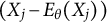 forms an uncorrelated sequence (Lemma 3). Therefore, Proposition 7 shows that a martingale factor model with bounded items which is convergently estimable to a non-degenerate
$T(\theta )$
 , and with a mean conditional variance that converges, has a reliability which goes to one at the Spearman–Brown rate.
3.1 Sufficient conditions for convergent estimability
Here, we use standard convergence results (see, e.g., Billingsley, Reference Billingsley1995, Section 16) to provide two sufficient conditions for convergent estimability that are based on an item sequence being consistently estimable. These sufficient conditions are based on assuming that
$\vartheta \mapsto E_\vartheta [\bar X_J]$
 converges to a function pointwise. Conditions that imply this pointwise convergence are given in Section 3.2.
Lemma 5. For an item sequence X, suppose that
$\bar X_{J} = T_J(\theta ) + o_{\text {a.s.}}(1)$
 for a function sequence
$(T_J)$
 which converges pointwise to a function T. Then X is convergently estimable.
Under a monotonicity assumption, we provide the following sufficient condition for convergent estimability. Recall that if X is an unconditionally consistently estimable item sequence and
$T_J(\theta )=T(\theta )+o_P(1)$
 , then
$\bar X_{J} = T(\theta ) + o_P(1)$
 .
Lemma 6. For an item sequence X, suppose that
$\bar X_{J} = T_J(\theta ) + o_P(1)$
 , where for each sufficiently large J we have that
$\vartheta \mapsto T_J(\vartheta )$
 is monotone, and that the function sequence
$T_J$
 converges pointwise to a function
$T(\vartheta )$
 . If
$\theta $
 is univariate and T is continuous, then X is convergently estimable.
3.2 Items with conditional expectations parameterized by sequences which fulfill a law of large numbers result
We now present a general technique which can show that
$T_J$
 converges pointwise. Choose, for each
$j\ge 1$
 , a measurable version
$m_j:\mathbb {R}^{d_\theta }\to \mathbb {R}$
 , where
$d_\theta $
 is the dimension of
$\theta $
 , such that almost surely,
$ m_j(\theta )=E[X_j|\theta ]$
 . Such versions exist by Kallenberg (Reference Kallenberg2021, Theorem 8.1).
We may always represent
$m_j(x)=H(x,\beta _j)$
 for a function H and a sequence
$(\beta _j)$
 ; for example, one may take
$d_\beta =1$
 ,
$\beta _j=j$
 , and
$H(x,j)=m_j(x)$
 . This representation is, however, non-unique, and for parametric models we can often express H in terms of standard parameter sequences.
Example 1. Consider a threshold model
$X_j = I \{ \varepsilon _j \leq \theta \}$
 , where
$I\{\cdot \}$
 denotes the indicator function,
$(\varepsilon _j)$
 and
$\theta $
 are independent, and
$\varepsilon _j \sim N(\mu _j, \sigma _j^2)$
 with
$\sigma _j>0$
 for all j. Let
$\Phi $
 denote the cumulative distribution function of the standard normal distribution. Then
$ E[X_j|\theta ] = \Phi ((\theta - \mu _j)/\sigma _j) $
 , so we may take
$\beta _j = (\mu _j, \sigma _j)$
 and
$ H(x, (\mu _j, \sigma _j)) = \Phi \big ( (x - \mu _j)/\sigma _j \big ). $

We may often approximate the average
$T_J(\vartheta ) = J^{-1} \sum _{j=1}^{J} H(\vartheta , \beta _j)$
 by an integral, implying the pointwise convergence assumed in Lemmas 5 and 6.
Definition 6. A non-random sequence
$(\beta _j)$
 of
$d_\beta $
 -dimensional vectors is said to fulfill the law of large numbers property if, for any bounded continuous function G, we have that
$ J^{-1} \sum _{j=1}^{J} G(\beta _j) = \int _{\mathbb {R}^{d_\beta }} G(t) \, \mathrm {d} F_\beta (t) + o(1), $
 for some probability distribution
$F_\beta $
 , where
$d_\beta = \dim (\beta _j)$
 .
Technically, Definition 6 says that the empirical probability measure of
$(\beta _j)_{j=1}^J$
 converges weakly (Klenke, Reference Klenke2020, Definition 13.12) to some probability measure. There is a large class of item-parameter sequences for which this property is natural. This includes sequences with a finite number of possible outcomes whose relative proportions stabilize as the sequence grows (
$F_\beta $
 is then a discrete distribution), many low-discrepancy or quasi-Monte Carlo constructions (Niederreiter, Reference Niederreiter1992, Chapters 2 and 3), and the random-item setting considered in Appendix E of the Supplementary Material after conditioning on the realized item-selection sequence. Showing the convergence of such sums to an integral from first principles may be highly non-trivial. Variants of Definition 6 are a standard tool for dealing with limits of non-identically distributed random variables. See, e.g., the asymptotic framework of Section 2.2 in Claeskens and Hjort (Reference Claeskens and Hjort2008) and e.g. Ploberger and Krämer (Reference Ploberger and Krämer1996, Assumption A1), and many similar papers in econometrics).
Under parametric assumptions,
$\beta _1, \ldots , \beta _{J}$
 may be estimated empirically. Any observed stability among such estimates must be interpreted with caution, as Definition 6 is asymptotic, and the stability is required to continue indefinitely for the law of large numbers property to hold. Substantive knowledge of the item sequence, such as it being generated by drawing at random from an infinite item pool, is required to justify the law of large numbers property.
The law of large numbers property can be recast as a between-form stability property similarly to Lemma 4. We assume that
$(\beta _j)$
 is bounded, which is the case in practice.
Lemma 7. Let
$(\beta _j)$
 be a sequence of
$d_\beta $
 -dimensional vectors fulfilling
$\sup _j |\beta _j| < c$
 . Then
$(\beta _j)$
 fulfills the law of large numbers property if and only if for every bounded continuous function G and every two sequences of nonempty sets
$A_J \subseteq \{1, \ldots , J\}$
 and
$B_L \subseteq \{1, \ldots , L\}$
 satisfying
$|A_J|/J \xrightarrow {} 1$
 and
$|B_L|/L \xrightarrow {} 1$
 , we have
$ \sup _{J,L \geq N} \left | \frac {1}{|A_J|}\sum _{j\in A_J} G(\beta _j) - \frac {1}{|B_L|}\sum _{j\in B_L} G(\beta _j) \right | \xrightarrow {} 0 $
 as
$N \xrightarrow {} \infty $
 .
Lemma 7 allows the psychometrician to think about the law of large numbers property as a between-form stability condition: as the number of items increases, averages of bounded continuous functions of the item parameters are asymptotically unchanged by removing a vanishing fraction of the items.
Since Definition 6 is asymptotic, it cannot be used to derive finite J bounds, such as those we considered earlier in the article. This may be improved with further assumptions. For example, when drawing items from an infinite item pool, one can derive finite-item guarantees based on the probability measure of the randomization device. We do not consider such refinements in the present article.
As a direct consequence of Definition 6 and Lemmas 5 and 6, we get the following conclusion. In its first statement, we recall that
$\bar X_{J} = T_J(\theta ) + o_{\text {a.s.}}(1)$
 if X is consistently estimable with exponential concentration (Proposition 1), which holds for bounded martingale factor models by Proposition 3 with
$\alpha _j\equiv 1$
 —and therefore also for bounded conditionally independent items by Proposition 2.
Theorem 1. For an item sequence X, suppose there exists a measurable function H and a sequence
$(\beta _j)$
 such that
$ E[X_j | \theta ] = H(\theta , \beta _j)$
 a.s. for every
$j\ge 1$
 , where
$(\beta _j)$
 follows the law of large numbers property, and suppose that for any given
$\vartheta $
 , the function
$b \mapsto H(\vartheta , b)$
 is bounded and continuous. Then X is convergently estimable with
$ T(\vartheta ) = \int _{\mathbb {R}^{d_\beta }} H(\vartheta , b) \, \mathrm {d} F_\beta (b), $
 as long as either of the following assumptions is fulfilled: (1) X is strongly unconditionally consistently estimable or (2) X is unconditionally consistently estimable,
$\theta $
 is univariate, and
$T_J(\vartheta ) = J^{-1} \sum _{j=1}^{J} H(\vartheta , \beta _j)$
 is monotone and T is continuous.
We now consider the conditionally independent case. For conditionally independent items, a representation of the form assumed in the upcoming result is available at the level of distributions by Lemma 1. The substantial assumption in the corollary is therefore that the parameter sequence fulfills the law of large numbers property.
Corollary 1. Suppose X is bounded and conditionally independent given
$\theta $
 , and has the same distribution as if
$X_j = \mathcal {H}(\theta , (U_j, \beta _j))$
 for
$j \geq 1$
 , where
$(U_j)$
 is a sequence of independent random variables that are uniform on
$[0,1]$
 and
$(U_j)$
 is independent of
$\theta $
 . Assume further that for any given
$\vartheta $
 , the function
$ t \mapsto \int _0^1 \mathcal {H}(\vartheta ,(u,t))\,\mathrm {d} u $
 is bounded and continuous. If
$(\beta _j)$
 fulfills the law of large numbers property, X is convergently estimable, with
$T(\vartheta ) = E \mathcal {H}(\vartheta , Q)$
 , where
$Q = (U,\beta )$
 is such that U and
$\beta $
 are independent, and where
$U \sim U[0,1]$
 and
$\beta \sim F_\beta $
 .
Example 2 (Example 1, continued)
We have
$X_j = I \{ \mu _j + \sigma _j \Phi ^{-1}(U_j) \leq \theta \}$
 , so that
$\mathcal {H}(x, (u, \beta _j)) = I \{ \mu _j + \sigma _j \Phi ^{-1}(u) \leq x\}$
 with
$\beta _j=(\mu _j,\sigma _j)\in \mathbb {R}\times (0,\infty )$
 . While
$t\mapsto \mathcal {H}(x,(u,t))$
 need not be continuous, Corollary 1 only requires continuity of
$ t = (t_m, t_s) \mapsto \int _0^1 \mathcal {H}(x,(u,t))\,\mathrm {d} u, $
 which holds since
$ E I \{ t_m + t_s \Phi ^{-1}(U) \leq x \} = \Phi [(x - t_m)/t_s] $
 is bounded and continuous on
$\mathbb {R}\times (0,\infty )$
 . Hence, if
$(\beta _j)$
 fulfills the law of large numbers property, Corollary 1 implies
$\bar X_{J} = T(\theta ) + o_P(1)$
 , with
$ T(\vartheta )= E \mathcal {H}(\vartheta , Q) = \int _{\mathbb {R}^2} \Phi [(\vartheta - t_m)/t_s] \, \mathrm {d} F_{\beta }(t_m, t_s). $

In Appendix E of the Supplementary Material, we show that, after conditioning on the realized item-selection sequence, randomly selecting from a large pool of conditionally independent items yields an item sequence that is conditionally independent and parameterized by a sequence that fulfills the law of large numbers property, thereby providing a more substantial illustration of Corollary 1.
4 Theoretical applications
Here, we gather applications of the theory developed above, some of which are illustrated numerically in Section 5.
4.1 Unconditional and person-specific confidence intervals for the true score
We now consider confidence intervals for a respondent’s true score, computed based only on that respondent’s answers.
We only consider coverage rates under the unconditional probability measure, thereby taking into account that respondents are sampled at random, which is often the relevant perspective (see Chang & Stout, Reference Chang and Stout1993, Section 4, p. 50 and Holland, Reference Holland1990, p. 581 onward).
For a given
$0 < \alpha < 1$
 , let
$z_\alpha =\Phi ^{-1}(1-\alpha /2)$
 , where
$\Phi $
 is the cumulative distribution function of the standard normal distribution. Under the conditions of Proposition 4, we have that
$ \lim _{J \xrightarrow {} \infty } P\!\left ( T_J(\theta ) \in \bar X_{J} \pm z_\alpha \hat V_{J}^{1/2}/\sqrt {J} \right ) = 1 - \alpha , $
 where
$\bar V_J(\theta ) = J^{-1} \sum _{j=1}^J \text {Var}\,_\theta X_j$
 , and
$\hat V_{J}$
 is assumed to fulfill
$\hat V_{J} = \bar V_{J}(\theta ) + o_P(\bar V_J(\theta ))$
 . Finding such a consistent variance estimator may be possible under weak assumptions, for example, using methods such as those in Douglas (Reference Douglas1997) and Ramsay (Reference Ramsay1991). While this would be highly advantageous, it requires large J and a large number of respondents n. We here restrict attention to the less studied case where n is small and may even be
$1$
 , and use a variance estimator that is inconsistent though with a known positive bias.
For a fixed
$0 < \alpha < 1$
 , let
$z_\alpha =\Phi ^{-1}(1-\alpha /2)$
 and consider the confidence interval

If the items were independent and identically distributed, this interval would have asymptotic nominal coverage, but under a martingale factor model (and hence for conditionally independent items) that satisfies the assumptions of Proposition 4, the interval is instead asymptotically conservative.
Theorem 2. Suppose the assumptions of Proposition 4 hold with
$\alpha _j = 1$
 for all j, and assume in addition that
$0 \le X_j \le K$
 for all
$j\ge 1$
 . Let
$Z \sim N(0,1)$
 be independent of
$\theta $
 , and define
$ W_J(\theta ) = J^{-1}\sum _{j=1}^J \big (E_\theta [X_j]-T_J(\theta )\big )^2$
 , and
$ B_J(\theta ) = \bar V_J(\theta )/(W_J(\theta )+\bar V_J(\theta )), $
 where
$\bar V_J(\theta ) = J^{-1} \sum _{j=1}^J \text {Var}\,_\theta X_j$
 . Assume that
$B_J(\theta )>0$
 almost surely for all sufficiently large J. Then, as
$J\xrightarrow {} \infty $
 ,
$ P \left ( T_J(\theta ) \in I_J \right ) = 1-\alpha + 2 P \left ( z_\alpha \leq Z \leq z_\alpha B_J(\theta )^{-1/2} \right ) + o(1). $

We revisit this result in Section 4.1.3 where we introduce assumptions that lead to a limit of
$B_J(\theta )$
 as J increases, yielding a concrete expression for the asymptotic coverage of
$I_J$
 .
4.1.1 Small J improvements: A hybrid approach using a Clopper–Pearson-type argument
While Theorem 2 is an asymptotic result, its empirical relevance concerns finite J. We now consider finite-J improvements. An important limitation of
$I_J$
 is that if
$s_J = 0$
 , the resulting singleton interval will almost surely not contain
$T_J(\theta )$
 . In short tests, it is highly likely that some candidates answer all questions either correctly or incorrectly, yielding no empirical variance. This indicates that
$I_J$
 should not be used in such cases.
Clopper and Pearson (Reference Clopper and Pearson1934) provide a finite-J conservative confidence interval for independent and identically distributed binary observations that is valid and non-singleton even when
$s_J = 0$
 . From Hoeffding (Reference Hoeffding1956, Section 5), Clopper–Pearson intervals are finite-J conservative as confidence intervals for the average success probability also in the non-identically distributed case. Under conditional independence, this means that the interval is a finite-J conservative confidence interval under
$P_\theta $
 for the true score. Taking expectations, this holds also under P. However, numerical experiments reported in Section 5.3 show that the Clopper–Pearson interval is excessively conservative unless J is large. In our simulations, the hybrid approach we now propose outperforms Clopper–Pearson for all J. Further, the hybrid approach can be used for non-binary items, and holds under martingale factor models and does not require the stricter assumption of conditional independence. We therefore do not further consider the Clopper–Pearson interval in the main text.
The hybrid interval starts by considering the case
$X_1 = X_2 = \cdots = X_J = x$
 . For
$K=1$
 , the Clopper–Pearson interval is
$[0, 1 - c_{\alpha ,J}]$
 when
$x=0$
 and
$[c_{\alpha ,J}, 1]$
 when
$x=1$
 (Thulin, Reference Thulin2014, p. 820), where
$c_{\alpha ,J} = (\alpha /2)^{1/J}$
 . These intervals have endpoints that are convex combinations of the common value x and the interval endpoints, and for
$x = 0, 1$
 are of the form
$ [c_{\alpha ,J} x + (1-c_{\alpha ,J})\cdot 0, c_{\alpha ,J}x + (1-c_{\alpha ,J})\cdot 1] = [c_{\alpha ,J}x, c_{\alpha ,J}x+(1-c_{\alpha ,J})]. $
 Let us therefore consider, for general
$K \geq 1$
 , intervals of the form
$[c_{\alpha ,J} x + (1-c_{\alpha ,J})\cdot 0, c_{\alpha ,J}x + (1-c_{\alpha ,J})\cdot K] = [c_{\alpha ,J}x, x + (K-x)(1-c_{\alpha ,J})]$
 . We obtain the following bound.
Proposition 8. Suppose that
$X=(X_1,X_2,\ldots )$
 follows a martingale factor model in
$\theta $
 and that
$0\le X_j\le K$
 almost surely for all j. Let
$0<\alpha <1$
 ,
$c_{\alpha ,J} = (\alpha /2)^{1/J}$
 , and let
$I_{\text {CP}} = \big [\,X_1 c_{\alpha ,J},\; X_1+(K-X_1)(1-c_{\alpha ,J})\,\big ]$
 . Then
$ P\!\left ( s_J=0,\; T_J(\theta )\notin I_{\text {CP}} \right )\le \alpha. $

The lengths of these intervals are
$|I_J| = 2z_\alpha s_J/\sqrt {J}$
 and
$|I_{\text {CP}}| = K(1-c_{\alpha ,J})$
 . Switching to
$I_{\text {CP}}$
 when
$s_J=0$
 creates a discontinuity in length as
$s_J \to 0$
 , where the length suddenly jumps to
$K(1-c_{\alpha ,J})$
 . This discontinuity reflects a finite-sample limitation of the normal approximation, and we therefore suggest a continuity-corrected hybrid interval

where
$\tilde s_J = \max (s_J,\eta _J^{\text {len}})$
 is chosen to preserve continuity, with

Numerical experiments reported in Section 5.3 show that for the data generating processes we consider, the hybrid approach is superior to
$I_J$
 and to a discontinuous hybrid approach using
$\tilde s_J = s_J$
 , and that this holds for all J.
In the proof of Theorem 2, we show that, conditionally on each admissible value of
$\theta $
 ,
$ s_J^2 = \bar V_J(\theta ) + W_J(\theta ) + o_P(\bar V_J(\theta )). $
 Moreover, the assumptions of the theorem imply
$J\bar V_J(\theta ) \to \infty $
 , whereas
$ (\eta _J^{\text {len}})^2 = O(J^{-1}). $
 It follows that
$P(s_J < \eta _J^{\text {len}}) \to 0$
 . Hence, for large J, the hybrid interval coincides with the asymptotic interval with probability tending to one, and therefore has the same asymptotic conservative coverage as
$I_J$
 . When
$s_J < \eta _J^{\text {len}}$
 ,
$I_J$
 is shorter than
$I_{\text {CP}}$
 ; the continuity bridge defining
$\tilde I_J$
 corrects this short-length regime without the excessive conservatism of finite-J conservative intervals such as the Clopper–Pearson interval of Clopper and Pearson (Reference Clopper and Pearson1934).
4.1.2 Some implications for ability ranking
Confidence intervals for true scores can be translated into ranking uncertainty measures when the true score is strictly increasing in ability. Related ideas are well known in nonparametric IRT, where sum or mean scores are used to order respondents under conditions implying stochastic ordering or ordinal sufficiency (see, e.g., Grayson, Reference Grayson1988; Hemker et al., Reference Hemker, Sijtsma, Molenaar and Junker1997; Ligtvoet, Reference Ligtvoet2012, Reference Ligtvoet2015; van der Ark, Reference van der Ark2005; van der Ark & Bergsma, Reference van der Ark and Bergsma2010; Zwitser & Maris, Reference Zwitser and Maris2016.)
First, consider two respondents with item processes
$(X_{1,j})$
 and
$(X_{2,j})$
 , latent variables
$\theta _1,\theta _2$
 , and true score functions
$T_{1,J}(\vartheta ) = T_{2,J}(\vartheta )$
 , which are strictly increasing. Let
$ d_j:=X_{2,j}-X_{1,j}$
 ,
$\bar d_J:=\frac {1}{J}\sum _{j=1}^J d_j$
 ,
$\Delta _J:= T_{2,J}(\theta _2)-T_{1,J}(\theta _1),$
 and
$ s_{\Delta ,J}^2:=\frac {1}{J-1}\sum _{j=1}^J (d_j-\bar d_J)^2. $

The following result can be generalized to martingale factor models, though this requires certain properties of the structure of conditional independence which we consider outside the scope of the present article. We therefore restrict attention to conditionally independent items.
Corollary 2. Assume that
$(X_{1,1}, X_{1,2}, \ldots )$
 is conditionally independent given
$\theta _1$
 , and that
$(X_{2,1}, X_{2,2}, \ldots )$
 is conditionally independent given
$\theta _2$
 . Suppose also that
$(\theta _1, X_{1,1}, X_{1,2}, \ldots )$
 is independent of
$(\theta _2, X_{2,1}, X_{2,2}, \ldots )$
 , that each
$X_{i,j}$
 is contained in
$[0,K]$
 for all
$i,j$
 , and that
$\theta _1, \theta _2$
 are univariate. Assume further that
$ \sum _{j=1}^J \text {Var}\,_{\theta _i}(X_{i,j}) \xrightarrow {} \infty $
 almost surely for
$i=1,2$
 . Then
$ I_{\Delta ,J}:=\left [\bar d_J \pm z_\alpha s_{\Delta ,J}/\sqrt {J}\right ] $
 is an asymptotically conservative
$1-\alpha $
 confidence interval for
$\Delta _J$
 . If
$L_J$
 denotes the lower endpoint of
$I_{\Delta ,J}$
 , then
$ P(\Delta _J\le 0,\ L_J>0)\le \alpha +o(1), $
 and declaring respondent 2 above respondent 1 in ability whenever
$L_J>0$
 has asymptotic error probability at most
$\alpha $
 .
Hybrid improvements for the interval in Corollary 2 as in Section 4.1.1 should be applied in practical work.
Second, consider n independent respondents. Let
$T_{i,J}$
 and
$I_{i,J}$
 denote the true score and a
$1-\tilde \alpha $
 confidence interval for respondent i, respectively. Since each interval
$I_{i,J}$
 is constructed solely from respondent i’s own data, by independence,
$ P\Big (\bigcap _{i=1}^n \{T_{i,J}\in I_{i,J}\}\Big ) = \prod _{i=1}^n P(T_{i,J}\in I_{i,J}). $
 Hence, for asymptotically conservative intervals, the simultaneous coverage probability is at least
$ (1-\tilde \alpha +o(1))^n = 1-\alpha +o(1) $
 when
$ \tilde \alpha =1-(1-\alpha )^{1/n}, $
 where here n is fixed and J increases.
4.1.3 Simplifications under consistent estimability
We now identify the limiting coverage probability for the confidence interval considered in Theorem 2 under consistent estimability, and a certain second moment convergence which can be justified in similar ways as convergent estimability.
Lemma 8. Suppose that
$ T_J(\theta ) = T(\theta ) + o_P(1), $
 that
$J^{-1} \sum _{j=1}^J E_\theta [X_j^2] = T^{(2)}(\theta ) + o_P(1), $
 and that
$ J^{-1} \sum _{j=1}^J \big (E_\theta [X_j]\big )^2 = M^{(2)}(\theta ) + o_P(1). $
 Also, assume
$T^{(2)}(\theta )-T(\theta )^2>0$
 with probability one. Then

Under eq. (8), and with the convention that
$B(\theta )^{-1/2}=\infty $
 on
$\{B(\theta )=0\}$
 , the coverage probability from Theorem 2 converges to
$1-\alpha + p_B$
 , where

This is close to
$1-\alpha $
 when
$B(\theta )$
 is concentrated around
$1$
 . A simple numerical illustration is given in Section 5.2.
4.2 Convergence of mean-score correlations
Here, we consider the empirical practice of using mean scores in correlation-based methods, such as factor analysis or structural equation models (see Bollen, Reference Bollen1989, for a textbook introduction to these models). This practice may be motivated by linear factor models of the form
$(X_1, \ldots , X_J)' = \Lambda \theta + u$
 , where
$\theta $
 is a vector,
$\Lambda $
 is a full column rank matrix, and
$\theta $
 is uncorrelated with u. Then, for suitably chosen linear transformations of the form
$H \cdot (X_1, \ldots , X_J)'$
 , such as a left inverse of
$\Lambda $
 , one obtains variables that are linear transformations of
$\theta $
 plus an error term. Under additional assumptions making this error small, the correlation matrix of
$H \cdot (X_1, \ldots , X_J)'$
 is therefore close to that of
$\theta $
 , which motivates this empirical practice.
This argument does not hold for item response models. In contrast, non-linear factor scores are required to consistently approximate
$\theta $
 . Yet we may inquire into what this common empirical practice approximates from a nonparametric IRT perspective, and we will show in the numerical illustrations that using mean scores as input into covariance models may work well, and even be superior to using misspecified parametric estimation methods.
Several models, including linear regression, factor analysis, and structural equation models are, under standard assumptions, dependent only on covariances and means (Bollen, Reference Bollen1989, Chapter 8). For standardized variables, the consistency of these methods only depends on correlations, which depend on pairs of items. We therefore consider only two scales in the following result.
Proposition 9. Let
$(X_j)_{j\ge 1}$
 and
$(Y_j)_{j\ge 1}$
 be two consistently estimable item sequences with latent variables
$\theta _X$
 and
$\theta _Y$
 . Let
$\bar X_{J_X}, \bar Y_{J_Y}$
 and
$T_{J_X}^{(X)}(\theta _X),T_{J_Y}^{(Y)}(\theta _Y)$
 be their respective mean and true scores. Assume that for some
$\varepsilon>0$
 ,
$ \sup _{j\ge 1}E|X_j|^{2+\varepsilon }<\infty , $
 and
$ \sup _{j\ge 1}E|Y_j|^{2+\varepsilon }<\infty. $

-
(1) Suppose there exist $\delta>0$
and
$J_0\ge 1$
such that for all
$J_X,J_Y\ge J_0$
, where
$\rho (\cdot ,\cdot )$
denotes Pearson correlation,
$ \text {Var}\,\!\big (T_{J_X}^{(X)}(\theta _X)\big )\ge \delta $
and
$\text {Var}\,\!\big (T_{J_Y}^{(Y)}(\theta _Y)\big )\ge \delta $
. Then, as
$J_X,J_Y\xrightarrow {} \infty $
,
$ \rho (\bar X_{J_X},\bar Y_{J_Y}) = \rho \!\big (T_{J_X}^{(X)}(\theta _X),T_{J_Y}^{(Y)}(\theta _Y)\big ) + o(1). $
-
(2) If, in addition, $(X_j)$
and
$(Y_j)$
are convergently estimable to
$T^{(X)}(\theta _X)$
and
$T^{(Y)}(\theta _Y)$
, respectively, and
$\text {Var}\,(T^{(X)}(\theta _X))>0$
,
$\text {Var}\,(T^{(Y)}(\theta _Y))>0$
, then
$ \lim _{J_X,J_Y\xrightarrow {} \infty }\rho (\bar X_{J_X},\bar Y_{J_Y}) = \rho (T^{(X)}(\theta _X), T^{(Y)}(\theta _Y)). $
-
(3) Let Z be a random variable with $\text {Var}\,(Z)>0$
and
$E|Z|^{2+\varepsilon }<\infty $
. Assume that there exist
$\delta>0$
and
$J_0\ge 1$
such that
$\text {Var}\,(T_{J}^{(X)}(\theta _X))\ge \delta $
for all
$J\ge J_0$
. Then, as
$J\xrightarrow {} \infty $
,
$ \rho (\bar X_J,Z)=\rho \!\big (T_{J}^{(X)}(\theta _X),Z\big )+o(1). $
-
(4) If, in addition, $(X_j)$
is convergently estimable to
$T^{(X)}(\theta _X)$
and
$\text {Var}\,(T^{(X)}(\theta _X))>0$
, then
$ \lim _{J\xrightarrow {} \infty }\rho (\bar X_J,Z)=\rho (T^{(X)}(\theta _X),Z). $


Proposition 9 shows that inputting sum or mean scores into correlation methods will be approximately the same as inputting functions of their underlying latent variables. Proposition 9(1) and (2) show that this holds when comparing the correlation of two mean scores, and Proposition 9(3) and (4) show that this holds when inputting a mix of, for example, continuous explanatory variables and mean scores. Under convergent estimability, Proposition 9(2) and (4) identify the limit of mean-score correlations. Importantly, Proposition 9(1) and (3) identify what mean-score correlations approximate without assuming convergent estimability, that is, without making an assumption on a theoretical infinite item sequence.
Inference in structural equation models typically relies on fourth-order moments (see, e.g., Satorra, Reference Satorra1989), and extensions of Proposition 9 lead to the convergence properties also of higher-order moments. We consider this outside the scope of the present article.
As an illustration of Proposition 9, we study the phenomenon that mean-score correlations have been reported to have an absolute value less than the true latent correlation under normality, as also seen in the upcoming numerical illustrations. For large J, this effect is explained by Proposition 9: suppose
$(\theta _X, \theta _Y)$
 are jointly normal. Then
$|\rho (T^{(X)}(\theta _X), T^{(Y)}(\theta _Y))| \leq |\rho (\theta _X, \theta _Y)|$
 , as
$|\rho (\theta _X, \theta _Y)|$
 is the maximal correlation coefficient under normality (see, e.g., the discussion on maximal correlation in Klaassen & Wellner, Reference Klaassen and Wellner1997, Section 2). If
$(\theta _X, \theta _Y)$
 has a non-normal copula, there is no simple monotonic relationship between the magnitude of
$\rho (T^{(X)}(\theta _X), T^{(Y)}(\theta _Y))$
 and
$\rho (\theta _X, \theta _Y)$
 without further assumptions.
4.3 Nonparametric factor scores
In IRT, estimating
$\theta $
 is of practical importance, though it may be both computationally and theoretically difficult. Computationally, the difficulty lies in the non-linear optimization problems required, while theoretically, the difficulty lies in identifying realistic assumptions resulting in robust methods which perform well in realistic sample and item number settings.
Alternatively, we may consider the mean score as an ordinal proxy for
$\theta $
 , and map its empirical ranks to a chosen latent scale. This idea appears, for example, as ordinal ability estimation in Douglas (Reference Douglas1997) and Ramsay (Reference Ramsay1991) and is closely related to the equipercentile equating argument (see, e.g., Lord, Reference Lord1982). In our setting, convergent estimability provides a direct justification for such rank-based scoring rules under weak assumptions, without requiring estimation of item response curves.
Suppose X is convergently estimable to
$T(\theta )$
 and
$\vartheta \mapsto T(\vartheta )$
 is a strictly increasing map, and suppose
$\theta $
 is univariate and has a known distribution function G. Then for each person
$i \geq 1$
 in a random sample,

We may estimate
$F(t) = P(T(\theta ) \leq t)$
 with the empirical distribution function
$F_{n,J}(t)$
 based on independently sampled mean scores. Let
$P[\cdot ]_\theta $
 mean a probability, where only
$\theta $
 is considered random. When
$n,J$
 increase,
$F_{n,J}(\bar X_{i,J})$
 is close to

so that the NPFS
$\hat \theta _i = G^{-1}(F_{n,J}(\bar X_{i,J}))$
 is close to
$\theta _i$
 . To avoid boundary issues in evaluating
$G^{-1}$
 , we re-scale the standard empirical distribution function and work with

for
$x \geq \min _r \bar X_{r,J}$
 .
Proposition 10. Suppose that X is convergently estimable to
$T(\theta )$
 and
$\vartheta \mapsto T(\vartheta )$
 is a strictly increasing and continuous map, and
$\theta $
 is univariate and follows a known continuous distribution function G, which is such that
$G^{-1}$
 is continuous on
$(0,1)$
 . Suppose further that we have a random sample from the first J items with a sample size of n, where the ith mean score and latent variable are denoted
$\bar X_{i,J}$
 and
$\theta _i$
 , respectively. Then
$\hat \theta _i = G^{-1}(F_{n,J}(\bar X_{i,J})) = \theta _i + o_P(1)$
 as
$(n,J) \xrightarrow {} (\infty , \infty )$
 .
This method, which can be refined in various directions that we do not study here, is a large-J, large-n method. It does not require knowledge of the limiting function T, and it avoids item-parameter estimation and optimization once the latent distribution G has been specified.
While G is assumed known, this is also the case in most other methods, such as parametric IRT. An advantage of the analytical simplicity of
$\hat \theta $
 is that it provides a transparent analysis of what is estimated if G is misspecified. Indeed, suppose
$\theta _i$
 has distribution function H, though
$\hat \theta _i$
 erroneously assumes
$\theta \sim G$
 . Then by Proposition 10, we get
$\hat \theta _i = G^{-1}(F_{n,J}(\bar X_{i,J})) = G^{-1} \circ H \circ H^{-1}(F_{n,J}(\bar X_{i,J})) = G^{-1} \circ H (\theta _i) + o_P(1) = \tilde \theta _i + o_P(1)$
 , where
$\circ $
 is function composition and
$\tilde \theta _i = G^{-1} \circ H (\theta _i)$
 . Interestingly, since
$P(\tilde \theta _i \leq t) = P( G^{-1} \circ H (\theta _i) \leq t ) = P( \theta _i \leq H^{-1} \circ G(t)) = H \circ H^{-1} \circ G(t) = G(t)$
 , the erroneous assumption that
$\theta _i \sim G$
 in fact reaches a transformed latent variable where this assumption is fulfilled.
Sample covariances or correlations computed from the resulting NPFSs can be input into covariance methods and will, under conditions similar to Proposition 9, converge to the true covariance or correlation between latent variables. Section 5.4 provides a numerical illustration of this idea. In contrast to mean-score correlations, the resulting estimate is consistent.
As an illustration, recall the martingale factor model with generalized partial credit marginals considered in Remark 5 under the additional assumption that its parameter sequence fulfills the law of large numbers property (Definition 6). In contrast to standard parametric latent variable estimates, the NPFS of Proposition 10 requires neither nuisance parameter estimation nor optimization for its computation.
Corollary 3. Assume that
$(X_1,X_2,\ldots )$
 follows a martingale factor model in
$\theta $
 . We assume that
$\theta $
 is univariate, and that the conditional marginals satisfy eq. (6) with
$w_j\ge 0$
 for all j. Suppose that
$\theta $
 has a known continuous distribution function G, and that
$G^{-1}$
 is continuous on
$(0,1)$
 , and that we have a random sample from the first J items with sample size n, with mean scores
$\bar X_{i,J}$
 and latent variables
$\theta _i$
 as in Proposition 10. If the parameter sequence
$(\beta _j)$
 fulfills the law of large numbers property with limit distribution
$P_\beta $
 with cumulative distribution function
$F_\beta $
 , satisfying
$P_{\beta }(w>0)>0$
 , then
$ \hat \theta _i \;:=\; G^{-1}\!\Big (F_{n,J}(\bar X_{i,J})\Big )\;=\;\theta _i+o_P(1)$
 as
$(n,J) \xrightarrow {} (\infty , \infty )$
 .
5 Numerical illustrations
5.1 A simple analytical illustration for calculating a limiting mean-score correlation
Here, we consider a simple model class with parameters drawn from an infinite item pool and having a particularly simple limiting true score.
Proposition 11. Suppose that
$X_j = I\{\lambda \theta + \varepsilon _j> \tau _j \}$
 , where
$\lambda> 0$
 ,
$\psi>0$
 ,
$(\varepsilon _j)$
 are independent and identically distributed
$N(0,\psi ^2)$
 variables, and
$(\varepsilon _j)$
 is independent of
$\theta $
 and of
$(\tau _j)$
 . Suppose further that
$(\tau _j)$
 are independent and identically distributed
$U[-c,c]$
 variables for some number
$c> 0$
 . Then, conditional on the realized threshold sequence
$(\tau _j)$
 , the item sequence X is convergently estimable with respect to
$\theta $
 for almost every realization of
$(\tau _j)$
 , with
$ T(\vartheta ) = 1 - (2c)^{-1}\big [(c - \lambda \vartheta )\Phi ((c - \lambda \vartheta )/\psi ) - (-c - \lambda \vartheta )\Phi ((-c - \lambda \vartheta )/\psi )\big ] - \psi (2c)^{-1}\big [\phi ((c - \lambda \vartheta )/\psi ) - \phi ((-c - \lambda \vartheta )/\psi )\big ], $
 where
$\phi $
 is the density of the standard normal.
Figure 1(a) shows the limiting function T of Proposition 11 for
$c = 0.9, \lambda = 0.5 = \psi $
 . Its curvature induces a small bias into the mean-score correlations as an estimator of the latent correlation (see Figure 1(c)). In contrast, with
$c = 2.5$
 , the limiting function is almost exactly linear, see Figure 1(b), which in turn induces an almost consistent mean-score correlation, see Figure 1(d).
Illustrations for Proposition 11. For panels (c) and (d),
$(\theta _X, \theta _Y)$
 is jointly normal with specified correlation
$\rho $
 .

Figure 1 Long description
The image consists of four panels arranged in a two by two grid.
Top-left panel A. The x axis is labeled with the Greek letter theta and ranges from negative 3 to 3. The y axis ranges from 0.0 to 1.0. A black curve shows a sigmoidal S-shaped increase, starting near 0 at x equals negative 3 and approaching 1.0 at x equals 3.
Top-right panel B. The x axis is labeled with the Greek letter theta and ranges from negative 3 to 3. The y axis ranges from 0.2 to 0.8. A black line shows a perfectly linear increase from the bottom-left to the top-right of the plot area.
Bottom-left panel C. The x axis is labeled rho open parenthesis xi comma eta close parenthesis and ranges from negative 1.0 to 1.0. The y axis is labeled rho open parenthesis X bar comma Y bar close parenthesis and ranges from negative 1.0 to 1.0. A red dashed line labeled Truth represents a perfect diagonal from negative 1 to 1. A solid black line labeled Estimate follows a similar path but has a slightly shallower slope, crossing the red line at the origin.
Bottom-right panel D. This panel uses the same axes and labels as panel C. The red dashed Truth line and the solid black Estimate line are nearly identical, showing a much tighter fit and a steeper slope than in panel C, almost perfectly overlapping along the diagonal.
5.2 The limiting bias of the naive confidence interval for the true score
Consider items of the form
$X_j = I \{ \varepsilon _j \leq \xi \}$
 , where
$\xi \sim N(0,1)$
 and
$\varepsilon _j \sim N(\mu _j, \sigma _j^2)$
 , and where
$\xi , \varepsilon _1, \ldots $
 are mutually independent. Before any items are drawn, we sample
$\mu _1, \ldots , \mu _{J} \sim U[-1,0], \sigma _1, \ldots , \sigma _{J} \sim U[0.2, 10/6]$
 independently, which is as if we sample from a random item pool. While written as a threshold model, the items follow a two-parameter probit IRT model by the equivalence shown in, for example, Takane and De Leeuw (Reference Takane and De Leeuw1987).
We study the coverage of the confidence interval from Theorem 2. Lemma 8 identifies the asymptotic coverage rate as
$1-\alpha + p_B$
 for
$p_B$
 as in eq. (9). We numerically approximate
$p_B$
 to be
$0.01$
 , giving an asymptotic coverage rate of
$96 \%$
 , compatible with the simulation illustration given next.
5.3 A numerical illustration of the person-specific confidence intervals
We extend the numerical illustration from Section 5.2 to polytomous items using a normal-threshold model, which reduces to the binary setup when
$K=1$
 . Let
$\xi \sim N(0,1)$
 , and independently draw
$\sigma _j\sim U[0.2,10/6]$
 and
$\eta _j\sim N(0,\sigma _j^2)$
 for each
$j \geq 1$
 , independently of
$\xi $
 . Given ordered thresholds
$\tau _{j,1}<\cdots <\tau _{j,K}$
 , we let
$ X^{(K)}_j = \sum _{k=1}^{K} I\{\xi +\eta _j>\tau _{j,k}\}\in \{0,1,\ldots ,K\}. $
 Thresholds are chosen to avoid nearly empty categories: For each item j, we draw a central location
$m_j\sim U[-1,0]$
 and set the K thresholds to be equally spaced on
$[m_j-c,\;m_j+c]$
 with
$c=2.5$
 . We consider
$2,3,5,7,$
 and
$9$
 response categories. The resulting items are conditionally independent. In Appendix D.1 of the Supplementary Material, we show that the hybrid confidence interval is well-behaved also under a martingale factor model which is not locally independent when
$K \geq 2$
 .
We let J vary from
$2$
 to
$200$
 . For each J and for a fixed parameter sequence
$(m_j), (\sigma _j)$
 , we compute coverage rates with 10,000 repetitions for the asymptotic confidence interval in Theorem 2, as well as the hybrid interval described in Section 4.1.1. Since the coverage rates depend on the parameter draws of
$(m_j), (\sigma _j)$
 , we repeat this whole process
$500$
 times (each time generating new
$(m_j), (\sigma _j)$
 parameters as described above). We then obtain a distribution of coverage rates for each J and each method.
The mean, and the lower and upper
$2.5 \%$
 quantiles, of the coverage rate distributions of the hybrid and asymptotic method, as well as the Clopper–Pearson method for
$K=1$
 , are shown in Figure 2, and tabulated in Appendix F.3 of the Supplementary Material.
Coverage rates as functions of J. The mean and the lower and upper
$2.5 \%$
 quantiles of the rate distributions are indicated.

Figure 2 Long description
A two-panel line graph. Both panels share a horizontal x-axis labeled J ranging from 0 to 200 and a vertical y-axis labeled Coverage rate ranging from 0.85 to 1.00. A horizontal dashed line is fixed at 0.95.
Panel A is titled Unconditional coverage probabilities of the 95 percent hybrid confidence interval, and the Clopper-Pearson interval for K = 1. The data lines start near 1.00 at low J and decrease. Most lines (K = 2, 4, 6, 8) drop sharply before stabilizing just above 0.95. The line for K = 1 (asterisks) stays slightly below 0.95. A dashed line with open circles for K = 1 (C P) remains higher, around 0.97. Shaded regions represent the lower and upper 2.5 percent quantiles.
Panel B is titled Unconditional coverage probabilities of the 95 percent asymptotic conservative interval I sub J. The data lines start at low coverage rates (below 0.85) and increase asymptotically toward 0.95 as J increases. The line for K = 1 (asterisks) is the lowest, while lines for higher K values (2, 4, 6, 8) reach the 0.95 threshold faster. Shaded regions indicate the distribution spread.
Legends in both panels identify:
* Asterisk: K = 1
* Blue circle: K = 2
* Red triangle: K = 4
* Green square: K = 6
* Purple diamond: K = 8
* Open circle (Panel A only): K = 1 (C P)
In the present simulation setup, the hybrid method performs well already from around
$J \geq 13$
 . In contrast, the Clopper–Pearson method and the uncorrected asymptotic interval
$I_J$
 perform poorly: Clopper–Pearson is excessively conservative, while
$I_J$
 has poor performance when
$s_J$
 is small, which occurs at high rates for small J (see Appendix F.3 of the Supplementary Material).
The coverage rate of the hybrid method is slightly conservative for sufficiently large J and for the values of K considered here. For J = 5,000 and
$K = 1$
 , the mean coverage rate was found to be
$95.89 \%$
 , compatible with the asymptotic bias calculated in Section 5.2.
5.4 Latent correlation estimates: Mean-score correlations, NPFS correlations, and ordinal factor analysis—A simple numerical illustration
We consider a standard threshold-based ordinal factor model with binary items, given by

for
$k=1,\ldots ,J$
 and
$j=1,\ldots ,J$
 (see Jöreskog, Reference Jöreskog1994, for background). The error terms
$(\epsilon ^{(X)}_{k})$
 and
$(\epsilon ^{(Y)}_{j})$
 are assumed mutually independent and also independent of the latent variables
$(\xi ,\eta )$
 . Under latent normality, this ordinal factor model is equivalent to a normal-link IRT model (Takane & De Leeuw, Reference Takane and De Leeuw1987).
In applied work, one is often interested in the latent correlation
$\rho = \rho (\xi ,\eta )$
 , perhaps as input to estimate a structural equation model. Under joint normality of
$(\xi , \eta )$
 and the error terms,
$\rho $
 can be estimated by fitting a factor model to the empirical tetrachoric correlations (Jöreskog, Reference Jöreskog1994). We call this the ordinal factor model estimator. In this illustration, we compare three estimates of
$\rho $
 : the ordinal factor model estimator, mean-score correlations, and correlations between the NPFSs of Section 4.3.
The NPFS requires knowledge of the marginal distributions of
$\xi $
 and
$\eta $
 . These marginals will be kept standard normal, and the non-normal scenarios we consider change only the copula of
$(\xi , \eta )$
 . The mean-score correlation does not rest on explicit distributional assumptions. In contrast, the ordinal factor model estimator requires latent joint normality and is generally inconsistent outside this assumption (Foldnes & Grønneberg, Reference Foldnes and Grønneberg2020, Reference Foldnes and Grønneberg2022). Even when all empirically testable normality assumptions for the latent variables appear to hold, latent normality does not need to hold, and model-based correlation estimates may deviate substantially from their population values under non-normality (Grønneberg & Foldnes, Reference Grønneberg and Foldnes2024). Latent non-normality is empirically relevant, as illustrated in Grønneberg and Foldnes (Reference Grønneberg and Foldnes2024), who applied a test for underlying normality from Grønneberg et al. (Reference Grønneberg, Moss and Foldnes2020) to a collection of psychometric data, and found that latent normality was strongly rejected for the seven psychometric datasets they considered. Testing for latent non-normality is not commonly done in practical applications even when using estimators that rest on this assumption.
For the simulations, we fix factor loadings
$\lambda _j^{(X)}=\lambda _j^{(Y)}=0.5$
 and set the error-term standard deviations also to
$0.5$
 . Thresholds
$\tau _j^{(X)}$
 and
$\tau _j^{(Y)}$
 are drawn once, uniformly from
$[-0.9,0.9]$
 , and kept constant across replications. In contrast to Section 5.3, we do not consider re-drawing the thresholds and redoing all the simulations per drawn threshold configuration, as this would be computationally too demanding due to the tetrachoric correlation calculations.
Extending the threshold range to
$[-2.5,2.5]$
 would significantly improve the performance of the mean-score correlation approach, as seen in Section 5.1. We did not consider this setup here, as it makes some item pairs so strongly dependent that the tetrachoric correlations become numerically unstable.
We consider
$\rho $
 either equal to
$0.8$
 or
$0.5$
 . A latent correlation of
$0.5$
 is common in practice, while a strong correlation of
$0.8$
 emulates cases where tests of unidimensionality are relevant, that is, that it is of interest to test whether
$\eta $
 and
$\xi $
 coincide. Further, we consider non-normal latent variables as described below, and normal latent variables. We consider normally distributed latent data only for
$\rho = 0.8$
 , as the mean-score correlations with normal latent variables were investigated systematically in Section 5.1, and the model-based approach is well-known to perform well under normality.
For the non-normal scenarios,
$(\xi , \eta )'$
 has standard normal marginals and the non-normal Joe copula with parameters chosen via the R-package covsim (Grønneberg et al., Reference Grønneberg, Foldnes and Marcoulides2022) to achieve the target correlation
$\rho $
 (
$0.5$
 or
$0.8$
 ). This type of copula-induced non-normality is known to detrimentally affect ordinal factor analysis (Foldnes & Grønneberg, Reference Foldnes and Grønneberg2020). Furthermore, the item error terms
$\epsilon ^{(X)}_{k}$
 are drawn from a
$\chi ^2_2$
 -distribution, and
$\epsilon ^{(Y)}_{j}$
 from a log-normal distribution, both subsequently scaled and shifted to have a mean of zero and a standard deviation of
$0.5$
 .
We generate data for
$n=3{,}000$
 respondents and set
$J=50$
 items per scale. Each distributional configuration is replicated
$1{,}000$
 times. For
$50$
 binary items per scale, computing the
$4{,}950$
 unique tetrachoric correlations for each replication is computationally intensive, and the resulting correlation matrix is frequently non-positive-definite (occurring in
$37.4\%$
 of the replications in the non-normal,
$\rho =0.80$
 case; for comparison, the corresponding rates are
$0.4\%$
 under normality with
$\rho =0.8$
 and
$0.3\%$
 in the non-normal,
$\rho =0.5$
 case). When a non-positive-definite matrix occurs, we apply the nearPD function from the R Matrix package (Bates et al., Reference Bates, Maechler and Jagan2024) to find the closest positive definite matrix before passing it to lavaan (Rosseel, Reference Rosseel2012). For ordinal data estimated via tetrachoric correlations, either diagonally weighted least squares (DWLS) or unweighted least squares (ULS) are recommended (Li, Reference Li2016; Forero et al., Reference Forero, Maydeu-Olivares and Gallardo-Pujol2009) when fitting factor models. We choose the ULS option in lavaan, as the DWLS option requires the additional computation of the asymptotic covariance matrix of the vectorized tetrachoric correlation matrix.
The mean absolute errors (MAEs) for each condition are shown in Table 1. Sampling distributions are shown in Appendix F.1 of the Supplementary Material; the appendix figures illustrate the bias directions discussed below.
Mean absolute errors for three estimators of the latent correlation based on 1,000 replications with
$n=3{,}000$
 and
$J=50$
 items per scale

Table 1 Long description
The table consists of four columns and four rows including the header.
Header Row:
- Estimator
- Normal, rho = 0.8
- Non-normal, rho = 0.8
- Non-normal, rho = 0.5
Row 1 (Ordinal factor model):
- Normal, rho = 0.8: 0.006 (bold-faced)
- Non-normal, rho = 0.8: 0.076
- Non-normal, rho = 0.5: 0.034
Row 2 (Nonparametric factor score):
- Normal, rho = 0.8: 0.042
- Non-normal, rho = 0.8: 0.022
- Non-normal, rho = 0.5: 0.014 (bold-faced)
Row 3 (Mean-score):
- Normal, rho = 0.8: 0.043
- Non-normal, rho = 0.8: 0.018 (bold-faced)
- Non-normal, rho = 0.5: 0.025
A note indicates that bold-faced values represent the best performing method for each condition.
Note: The best performing method is bold-faced.
We first consider the high-correlation scenario (
$\!\! \rho =0.8$
 ). Under latent normality, the ordinal factor model estimator performs as expected (MAE = 0.006) and outperforms the sum-score estimator and the NPFS, both of which exhibit downward bias (MAE = 0.042 and 0.043, respectively). However, when the normality assumption is violated, ordinal factor analysis substantially overestimates the latent correlation (MAE = 0.076). In contrast, the mean-score estimator, while remaining slightly conservative, is far more accurate under non-normality (MAE = 0.018), and slightly more accurate than the NPFS (MAE = 0.022).
In the moderate correlation scenario (
$\rho = 0.5$
 ) under non-normality, ordinal factor analysis maintains a positive bias (MAE = 0.034), whereas the sum-score estimator is slightly negatively biased but considerably more precise (MAE = 0.025). The best performing method is the NPFS, which is close to unbiased (MAE = 0.014).
Although this small illustration has limited external validity, it demonstrates that even when a binary factor model structure is correctly specified, the simple mean-score correlation can outperform a standard parametric estimator when its underlying distributional assumptions are violated, and that the NPFS estimator either performs similarly or better than the mean-score correlation. We note here that NPFS is applied with the correct latent variable distribution, which is in contrast to the ordinal factor model, and that the mean score does not directly rely on such a specification. Finally, the performance of the mean-score correlation is driven by the formula of the true score, which except under strong assumptions cannot be estimated (though with strong assumptions, it can be estimated as illustrated in Appendix F.2 of the Supplementary Material).
6 Conclusion
This article studied two asymptotic questions for mean scores under weak latent-variable assumptions: when the observed mean score approximates the true score of the administered form, and when form-specific true scores stabilize as the number of items grows. Our main theoretical contributions are the introduction of martingale factor models, which for polytomous items weaken conditional independence to a conditional-mean restriction while still yielding concentration and, under weak assumptions, asymptotic normality results for bounded items, and our analysis of convergent estimability via sufficient conditions based on a law of large numbers property for item-parameter sequences.
These results identify a regime in which mean scores admit a controlled large-form interpretation: first as approximations to form-specific true scores, and, under additional convergence conditions, as estimators of a limiting function of the latent variable. The later parts of the article, including the confidence-interval construction, the discussion of large-form mean-score correlations, the NPFS, and the numerical studies, are consequences and illustrations of this core theory and not general methodological recommendations.
The results also clarify what our results do not show. They do not justify unrestricted use of mean scores as substitutes for well-supported parametric methods, nor do they imply that mean-score correlations generally recover latent correlations. As shown in the article, mean-score correlations typically converge to correlations between functions of latent variables, and stronger assumptions are needed for calculating how close these correlations are to the latent correlations. When reasonable parametric models are substantively justified and empirically adequate, they should therefore remain the first choice in applications. At the same time, because parametric assumptions can be restrictive, incompletely tested, or violated in practice (Foldnes & Grønneberg, Reference Foldnes and Grønneberg2020, Reference Foldnes and Grønneberg2022; Grønneberg & Foldnes, Reference Grønneberg and Foldnes2024; Grønneberg et al., Reference Grønneberg, Moss and Foldnes2020; Moss & Grønneberg, Reference Moss and Grønneberg2023), our results provide a weak-assumption benchmark for understanding what large-form mean scores can and cannot support.
The article also has clear limitations. The methodological components require further study under wider simulation setups, and our numerical illustrations are limited in scope and are not intended as comprehensive validations of the methods. Also, practical psychometric theory is required to build robust justifications of the substantive assumptions of the methods we consider in the article. Another limitation is that we mainly rely on increasing-item asymptotics: the martingale factor model assumption is non-asymptotic, and non-asymptotic results can be developed for this model class, as exemplified by Proposition 3 (exponential concentration) and Proposition 8 (Clopper–Pearson generalization for
$s_J = 0$
 ). Further, we leave several psychometrically important issues for future work, including broader forms of conditional dependence, practical modeling within martingale factor models, further work on diagnostics of the martingale factor model property, response-time extensions, and systematic treatment of planned and unplanned missingness.
The contribution of the article is to make precise a weak-assumption setting in which mean scores track true scores and, under additional stability conditions, admit a coherent limiting interpretation. This separates conditions under which mean scores are defensible from conditions under which stronger psychometric assumptions are needed.
Supplementary material
The supplementary material for this article can be found at https://doi.org/10.1017/psy.2026.10135.
Data availability statement
All source code and data are included in the supplied OSF repository: https://osf.io/s5gwx.
Funding statement
The author declares that no specific funding has been received for this article.
Competing interest
The author declares none.
Declaration of use of AI tools
In the preparation of this manuscript, the author used ChatGPT (GPT-5.4, OpenAI) in the writing process, and for generating preliminary code for the numerical illustrations. The code was edited and quality checked by the author. The author takes full responsibility for the final integrity, accuracy, and content of the published work.
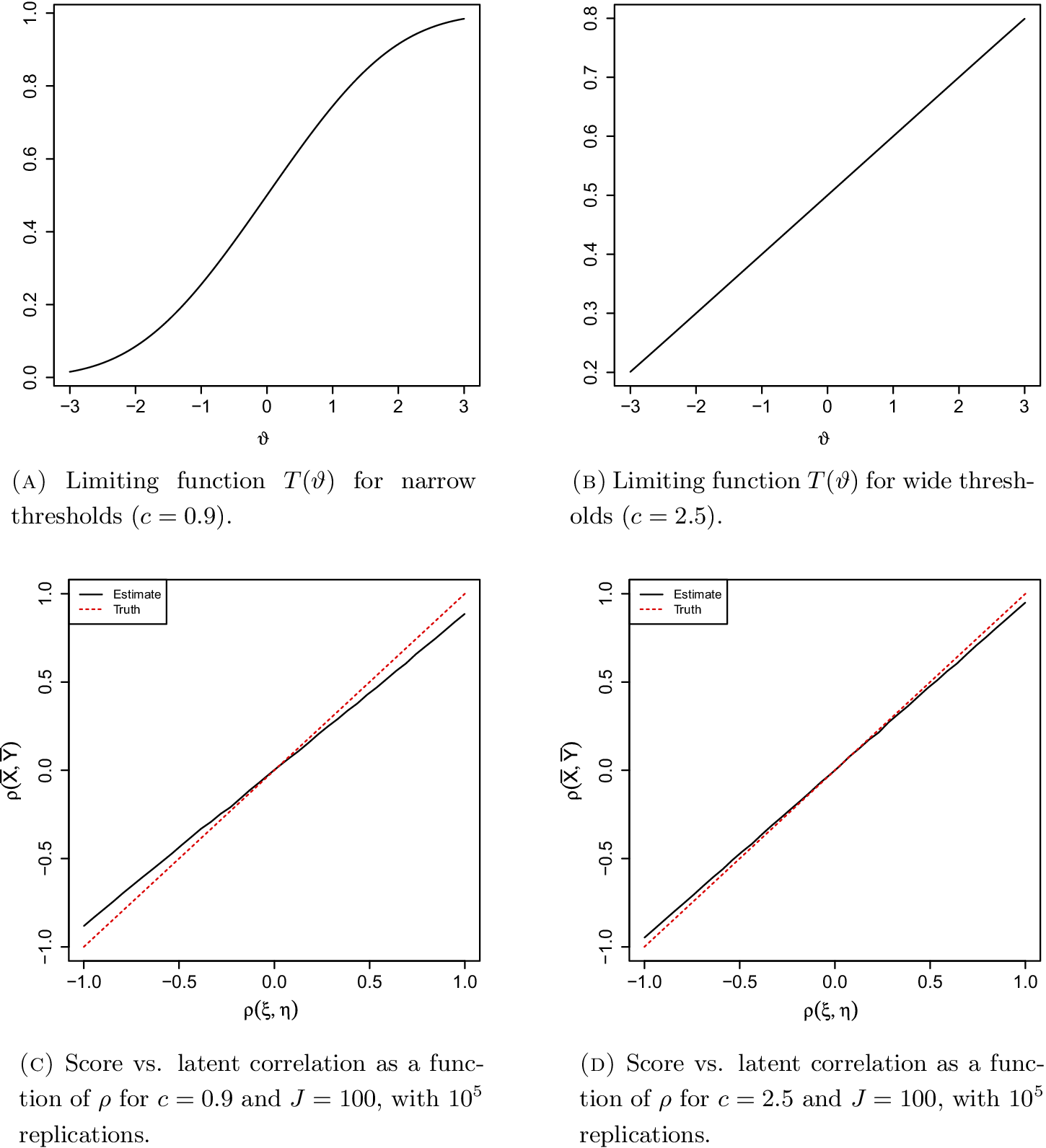


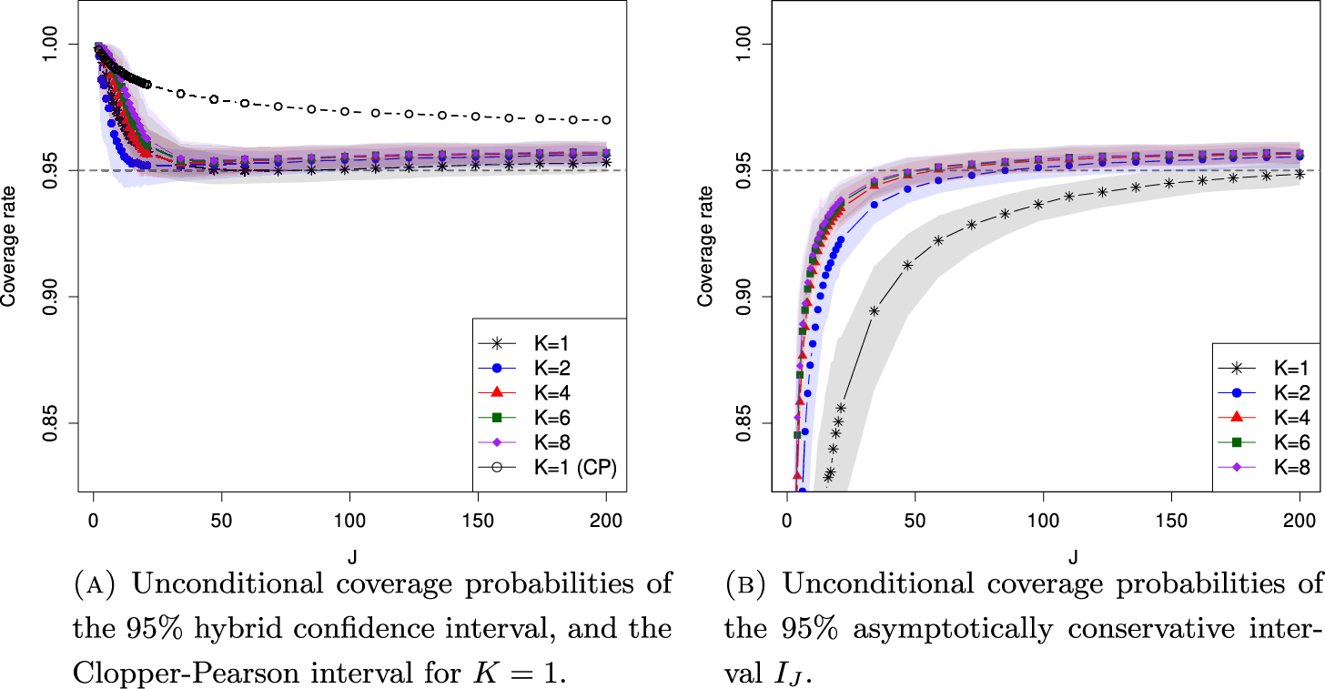




 Open access

