II. OVERVIEW OF CLASSICAL THEORY

In the classical theory [Reference Westcott1, Reference Blachman2], a real non-linear function f represents the instantaneous input-to-output transfer characteristic, e.g. a voltage transfer V _out = f(V _in).

When applying a sinusoidal input signal: V _in = a cos (ωt + φ) = a cos (θ), the output signal is composed of harmonics of the input frequency, especially a DC component (or harmonic 0) and a fundamental component (or harmonic 1)

(1)$$V_{out}=f\lpar V_{in}\rpar =f\left[{a\cos \lpar \theta \rpar } \right]=\displaystyle{1 \over 2}f_0 \lpar a\rpar +\sum\nolimits_{m=1}^\infty {f_m \lpar a\rpar } .\cos \lpar m\theta \rpar .$$

Function f _m (a) is the amplitude of harmonic m in the output signal. It is obtained as the order m Chebyshev transform of f(u) = f[a cos (θ)]

(2)$$f_m \lpar a\rpar =\displaystyle{1 \over \pi }\int_{ - \pi }^{+\pi } {f\left[{a\cos \lpar \theta \rpar } \right]} \cos \lpar m\theta \rpar d\theta .$$

The output amplitude at fundamental frequency, f ₁ (a), always an odd function of a, is called the AM/AM curve. The fundamental gain curve, or describing function (DF), g(a) = f ₁(a)/a, is always an even function of a. The Chebyshev transform is a special case of the discrete Fourier transform: it is the discrete cosine transform of the output signal when the input signal is a cosine and so is periodic and even. Function f may be non-analytic. Mathematically, it can be any distribution for which the Chebyshev transform can be computed. However, the classical theory generally restricts itself to analytic functions and frequently to polynomials.

For a function f that is an integer power of the variable u: f(u) = u ⁿ, the transform is [Reference Blachman2]

(3)$$\eqalign{f_m \lpar a\rpar &=\displaystyle{1 \over \pi }\int_{ - \pi }^{+\pi } {\left[{a\cos \lpar \theta \rpar } \right]^n } \cos \lpar m\theta \rpar d\theta \cr & =2\left({\displaystyle{a \over 2}} \right)^n \displaystyle{{n!} \over {\left({\lpar n+m\rpar /2} \right)!\; \left({\lpar n - m\rpar /2} \right)!}}}.$$

Note that equation (3) is valid only for integer m of same parity as n, with 0 ≤ m ≤ n. The result of the integral is null in other cases. Power functions (or monomials) are therefore invariants of the Chebyshev transform: the transform of a power function is a power function with the same exponent. As a consequence, if the function f is a polynomial, then all its Chebyshev transforms are polynomials. Even (respectively odd) harmonics are given by the terms of even (respectively odd) powers of input signal. Consequently, the fundamental output amplitude, f ₁ (a), is given by a polynomial with only odd degree terms. In case of two or more carriers input, the intermodulation products around the fundamental carriers will have odd orders only. Finally, the gain curve, g(a) = f ₁ (a)/a, is an even polynomial of input amplitude (with only even degree terms) or an arbitrary polynomial of input signal power (when power is proportional to the square of the input signal: voltage, current or wave).

The interest of these invariants, as shown by Blachman [Reference Blachman3], lies in the possibility to iterate the Chebyshev transform (once or many times). This makes computation of intermodulation products easy for two-carrier and multicarrier signals. In addition, the Chebyshev transform can be inverted easily when approximated with a polynomial.

This presentation is limited to the AM/AM curve and real polynomials but AM/PM can easily be taken into account with complex coefficients polynomials as shown in [Reference Kaye, George and Eric6]. All of the results are formally the same. The AM/PM phase curve can then be modeled as an even function of input amplitude in the same way as the gain. The AM/AM and AM/PM curves are identical to the amplitude and phase of the sinusoidal-input DF in control theory [Reference Gelb and Vander Velde7]. The function depends only on signal amplitude and not on signal frequency when the non-linearity is memoryless (called static in control theory).

A drawback of the polynomial models is their rapidly divergent behavior as the input amplitude goes beyond the maximum input value that has been used while characterizing the amplifier. It can be a problem for telecom simulation where Gaussian noise or multicarrier input signals with high dynamic range (e.g. orthogonal frequency division multiplex (OFDM) signals) have peaks much higher than their average value [Reference Rapp8]. To overcome this drawback, without introducing a limiter, a number of analytic functions have been proposed as models such as trigonometric (or Fourier–Bessel) series decompositions, rational functions or the hyperbolic tangent. Saleh proposed a rational function model of travelling wave tubes [Reference Saleh9] that is widely used. Cann [Reference Cann10] proposed a model for solid-state power amplifiers (SSPA) in addition to limiters and hyperbolic tangents. Rapp [Reference Rapp8] used the Saleh model and also proposed a modified model for the SSPA. A more complete discussion of the SSPA models will be found in Schreurs et al. [Reference Schreurs, O'Droma, Goacher and Gadringer11].

To conclude, the main inferences of the classical analytical function theory are the following:

1. 1. Orders of intermodulation products around the fundamental signal output (i.e. the odd harmonic of order 1) are odd integers: 3, 5, 7, etc.

2. 2. A polynomial function will give only products of order lower or equal to its degree.

3. 3. In small signal operation, the level of an intermodulation product will follow a slope, in dB/dB, with respect to the input level, equal to an integer number.

   This slope equals the lowest degree in the polynomial that is higher or equal to the order of the intermodulation product.

   Generally, this is understood as: third-order intermodulation products have a slope of 3 dB/dB, fifth-order 5 dB/dB, and so on. However, if the third degree term in the polynomial is null, whereas the fifth degree term is not, then the third-order product would have a slope of 5 dB/dB.

III. SIMPLE NON-ANALYTIC MODELS

A number of simple non-analytic models are commonly used to represent real world device operations: threshold, limiters, class AB, B, and C amplifiers or detectors as illustrated Fig. 1.

Fig. 1.

Some ideal non-analytic models.

Owing to the lack of a general theory for non-analytic functions, the harmonic and intermodulation content at the output of such devices is in general computed directly for each case, using for example Fourier decomposition of square waves for the threshold function. No general rules have been drawn for the behavior of harmonics and intermodulation products.

Other work exists in this domain, particularly in control theory [Reference Gelb and Vander Velde7, Reference Clarke and Hess12], two-carrier or multicarrier input signal is taken into account with multiple-input DFs. They are used to linearize the system and express amplitudes of output signals at frequencies of input signal. Noise and intermodulation products at frequencies different from those of the input signal are considered generally as errors in linearization.

Piecewise linear, piecewise polynomials or cubic splines are used to model transistors measured curves such as drain voltage versus drain current curve as a function of gate voltage for simulation purposes but not to obtain closed form results. Examples of DFs for such non-analytic functions are given in [Reference Gelb and Vander Velde7, Reference Clarke and Hess12–Reference Pedro, Carvalho, Fager and Garcia14].

Blachman [Reference Blachman2] gives the Chebyshev transform of some non-analytic functions, for example, the product of a power function and Heaviside function H given by

(4)$$\eqalign{&f\lpar u\rpar =H\lpar u\rpar \cdot u^n \quad \Leftrightarrow \quad f\lpar u\rpar =u^n\comma \; \quad {\rm for}\quad u\gt 0 \cr & {\rm and}\quad f\lpar u\rpar =0\comma \; \quad {\rm for}\quad u \leq 0.}$$

Its transform is:

(5)$$f_m \lpar a\rpar =\left({\displaystyle{a \over 2}} \right)^n \displaystyle{{n!} \over {\Gamma \left({\lpar n+m/2\rpar +1} \right)\; \Gamma \left({\lpar n - m/2\rpar +1} \right)}}.$$

Note that the factorial functions in the denominator of (3) have been replaced by the Gamma function in (5) as m and n may not have the same parity and the arguments may become half-integer. Since the Heaviside function is neither odd nor even, it generates even and odd harmonics or products. In particular, the output includes all harmonic orders of parity opposed to that of the degree n, even for a constant (n = 0) or a linear polynomial (n = 1) and harmonics of the same parity as degree n up to n: m = n, n − 2, n − 4, ... with m ≥ 0.

IV. NEW INVARIANTS OF THE CHEBYSHEV TRANSFORM

In this paper, the presentation will be restricted to functions that are not smooth (not C ^∞ and so not analytic) only at the origin. By definition of smoothness (C ^∞), either the function or one of its derivatives is not continuous at the origin and higher-order derivatives are infinite or undefined. Such a function cannot be replaced by a polynomial or an integer series around 0, even in a small range. In Fig. 1, only the threshold function and the linear detector are in this case. A class B amplifier without limitation (half-wave rectifier) would also be in that case.

A non-linear function based on the terms given in (4) could be used to model a non-linear class B amplifier in the small signal range. A push–pull amplifier would be obtained by complementing the positive part of the function with its opposite for negative inputs, thus obtaining an odd function. Even degree parts of this non-linear function do not disappear as they would if it was forced to be analytical and they are the cause of non-analyticity.

This is obtained by replacing the Heaviside function in equation (4) by the sign function:

(6)$$F\lpar u\rpar ={\rm sign}\lpar u\rpar \cdot u^n=\left\{{H\lpar u\rpar - H\lpar - u\rpar } \right\}\cdot u^n .$$

The sign function is odd and the parity of function f above is opposed to that of exponent n.

Its transform is:

(7)$$f_m \lpar a\rpar =2.\, {\rm sign}\lpar a\rpar .\left({\displaystyle{a \over 2}} \right)^n \displaystyle{{n!} \over {\Gamma \left({\lpar n+m/2\rpar +1} \right)\; \Gamma \left({\lpar n - m/2\rpar +1} \right)}}.$$

Equation (7) is valid for all values of m with parity opposed to that of n. In consequence, there are no harmonics or products of order having the same parity as n. More importantly, equation (7) shows that powers of the input multiplied by sign function are invariants of the Chebyshev transform like classical monomials. The polynomial model is generalized as

(8)$$f\lpar u\rpar =P\lpar u\rpar +{\rm sign}\lpar u\rpar .Q\lpar u\rpar$$

P(u) and Q(u) are arbitrary polynomials of input signal u. Both may contain odd terms and even terms. Here, P(u) is the polynomial that would be used in the classical theory.

It is, however, more appropriate to depart from the classical theory and explicitly separate the function in odd and even parts, using different polynomials

(9)$$f\lpar u\rpar =P\lpar \left\vert u \right\vert \rpar +{\rm sign}\lpar u\rpar .Q\lpar \left\vert u \right\vert \rpar .$$

The model of the odd part of the device characteristic: sign(u).Q(|u|) is generally the only one that gives output in the useful RF bandwidth. The even part P(|u|) should be considered when interested by the DC component (harmonic 0) and second harmonic output or when the bandwidth is large compared to centre frequency. Invariants of the Chebyshev transform are

(10)$${\rm Even}\; {\rm invariants}\comma \; \; {\rm for}\; {\rm any}\; {\rm integer}\; n\colon\ f\lpar u\rpar =\left\vert u \right\vert ^n\comma$$

(11)$${{\rm Odd}\; {\rm invariants}\comma \; \; {\rm for}\; {\rm any}\; {\rm integer}\; n\colon\ f\lpar u\rpar ={\rm sign}\lpar u\rpar .\left\vert u \right\vert ^n .}$$

The Chebyshev transforms of these invariants are readily given by

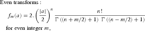(12)$$\eqalign{&{\rm Even}\; {\rm transforms}\colon \cr & \quad \; f_m \lpar a\rpar =2.\left({\displaystyle{{\left\vert a \right\vert } \over 2}} \right)^n \displaystyle{{n!} \over {\Gamma \left({\lpar n+m/2\rpar +1} \right)\; \Gamma \left({\lpar n - m/2\rpar +1} \right)}}\; \cr & \quad {\rm for}\; {\rm even}\; {\rm integer}\; m\comma}$$

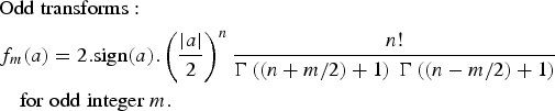(13)$$\eqalign{&{\rm Odd}\; {\rm transforms}\colon \cr & f_m \lpar a\rpar =2.{\rm sign}\lpar a\rpar .\left({\displaystyle{{\left\vert a \right\vert } \over 2}} \right)^n \displaystyle{{n!} \over {\Gamma \left({\lpar n+m/2\rpar +1} \right)\; \Gamma \left({\lpar n - m/2\rpar +1} \right)}}\; \cr & \quad {\rm for}\; {\rm odd}\; {\rm integer}\; m.}$$

Observe that the parity property (even or odd) is maintained throughout the Chebyshev transform. This implies that, as in the classical theory, orders of intermodulation products around the fundamental carrier signal output will be odd integers (3, 5, 7…) and will result only from the odd part of function f(u).

There are two important differences with the classical analytic model theory:

• • An odd invariant of any given degree (except an odd integer), will give harmonics and intermodulation products of all odd orders, instead of only orders lower than or equal to its degree (and similarly for even invariants).

• • Under small signal conditions, unlike in the classical analytic function theory, the output amplitude of a harmonic or product is no longer a monomial of the input amplitude with an integer exponent equal at least to its order m and with the same parity. The exponent (and so the slope in dB/dB) is equal to the degree n and not to the order m. In small signal conditions, a third order intermodulation product level does not always vary as a function of input level with a slope of 3 dB/dB. The slope could be any even integer (0, 2, 4…) as well as classically an odd integer at least equal to its order (3, 5…).

The classical constraints on the slopes of small signal intermodulation products (3 dB/dB, 5, 7, etc.) are not physical but an artifact due to the use of analytic invariants (the monomials), polynomials and analytic functions to describe or approximate the non-linearity.

Since the fundamental carrier output will result from the odd part of the characteristic, sign(u).Q(|u|), the AM/AM curve will be under the form: f ₁(a) = sign(a).R(|a|) with the polynomial R depending on the polynomial Q. The fundamental gain (or DF), an even function of a will be under the form

(14)$$g\lpar a\rpar =f_1 \lpar a\rpar /a={\rm sign}\lpar a\rpar .R\lpar \left\vert a \right\vert \rpar /a=R\lpar \left\vert a \right\vert \rpar /\left\vert a \right\vert .$$

As in the classical theory, one can use an even function to model the AM/PM curve and model its effect on the complex envelope of the signal: $\tilde u=a \cdot e^{j\theta}$. Function ${\rm sign}\lpar \tilde u\rpar$ is not defined on complex numbers and it must be replaced by $\tilde u/\left\vert {\tilde u} \right\vert =e^{j\theta}$.

Now, in light of the results above, a more general family of real and complex non-analytic invariants can be proposed, where the exponents can be fractional or real numbers p

(15)$${{\rm Even}\; {\rm invariants}\comma \; \; {\rm for}\; {\rm any}\; {\rm real}\; p\colon \; f\lpar u\rpar =\left\vert u \right\vert ^p \; {\rm or}\; f\lpar \tilde u\rpar =\left\vert {\tilde u} \right\vert^p}$$

(16)$$\eqalign{{\rm Odd}\; {\rm invariants}\comma \; \; {\rm for}\; {\rm any}\; {\rm real}\; p\colon\ f\lpar u\rpar &={\rm sign\lpar }u\rpar .\left\vert u \right\vert ^p \; {\rm or}\; \cr f\lpar \tilde u\rpar &=\tilde u.\left\vert {\tilde u} \right\vert ^{p - 1}}$$

The Chebyshev transforms of the above invariants are formally given by the same equations as (12) and (13) with integer n replaced by real p and factorial n! replaced by Gamma function Γ (p + 1). These non-analytic functions are also invariants of the Chebyshev transform and obey the same laws as the monomials provided that the real exponent p is higher than −1 to guarantee mathematical convergence of the series of transforms [Reference Blachman2].

V. PHYSICAL CONSTRAINTS ON NON-ANALYTICITY

For these invariants to be physical models of transfer functions, they must not create energy. This introduces additional constraints on the exponent

1. 1. The exponent must be positive or null to guarantee a finite output for null input for any physical device (an infinite output without input would not be acceptable).

2. 2. The exponent must be at least equal to 1 to guarantee a finite gain, and null output for null input, for a passive device (not necessary for an active device with a power supply).

For a positive real exponent p, the invariant is continuous but, except for integer p of the same parity as the invariant, its derivatives of order higher than p are not continuous at the origin and derivatives of order higher than p + 1 are indefinite. They are not smooth (C ^∞). A model based on these invariants will not be smooth, and so will not be analytic, at the origin. This is acceptable because the energy in the output signal is bounded when the input energy is bounded: bounded-in, bounded-out condition [Reference Gelb and Vander Velde7].

By using invariants (15) and (16) to model a device characteristic, one can explain small signal harmonics and IM products slopes of any positive or zero real value in dB/dB. For example, the output of a hard limiter or trigger, an active device with odd non-linearity and p = 0, consists of all odd harmonics and intermodulation products, each at a finite and constant level: all slopes are 0 dB/dB. The gain can be expressed by replacing the polynomial R in (14) by a sum or series of terms with real exponents p. This will give the designer much more flexibility for modeling practical measurement data, first by using odd and even degrees in polynomials of the modulus of the input signal, second by complementing the function with terms having real valued exponents.

The fact that a non-analytic at the origin model is better at modeling the behavior of a device is not a demonstration that the physical device itself has a discontinuity of some of its derivatives. Much more complicated analytic (or at least smooth) functions could be used to model the same behavior down to the level of thermal or quantum noise, where measurements would no longer be possible.

A simple example would be to replace the sign(u) function by the hyperbolic tangent: tanh(ku), with a large enough multiplicative coefficient k. The sign function is the mathematical limit of the hyperbolic tangent when k tends to infinity and it gives qualitative and easy to understand results that can be compared to measurements. The hyperbolic tangent model is continuous and infinitely derivable but the results are more complicated and would not permit easy iteration and inversion of the Chebyshev transform.

On the other hand, the simplicity and efficiency of a model based on non-analytic at the origin functions may be a good reason to examine some physical processes and try to find demonstrations, based on physics, of the reality or not of the discontinuity at the origin.

VI. BEHAVIOR OF CHEBYSHEV TRANSFORM INVARIANTS

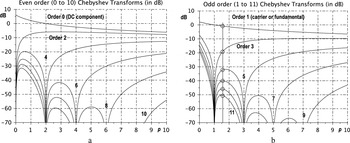
The output level of harmonics for a sinusoidal input (or equivalently IM products for two-carrier input) as a function of real exponent p are shown in Fig. 2 for the even parity and odd parity invariants (15) and (16).

Fig. 2.

Harmonics (or products) levels as a function of real exponent p in power function: (a) even order (0 to 10) transforms of even functions of type f(u) = |u|^p (b) odd order (1 to 11) transforms of odd functions of type f(u) = sign(u).|u|^p

In the case of integer exponents, harmonics or products disappear, in agreement with the classical theory, when they have the same parity as the exponent and strictly higher order. The curves are continuous functions of p, they only seem to be discontinuous on a graph in dB.

VII. ANALYSIS OF SOME MEASUREMENT RESULTS

A) Passive devices: antennas and filters

Many authors [Reference Chapman, Rootsey, Poldi and Davison15–Reference Hartman18] have reported even integer and/or non-integer slopes for odd order intermodulation products in passive devices such as antennas, filters and lines. These slopes were either explicitly presented as unexplained or supposed to be measurement errors.

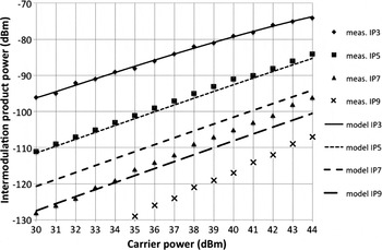
The authors in [Reference Shitvov, Zelenchuk and Schunchinsky16] measured passive intermodulation products of orders 3, 5, 7, and 9 in a micro strip line with 14 dB input level range around 900 MHz. They report slopes between 1.6 and 2.5 dB/dB for third-order to ninth-order IM products. Ratios of successive products are: I3/I5 = 14 dB, I5/I7 = 15 dB and I7/I9 = 10 dB. They also report slopes between 2 and 2.9 dB/dB on two different coplanar waveguide lines. They did not give an explanation for these unconventional values. Measurement data from [Reference Shitvov, Zelenchuk and Schunchinsky16] is presented in Fig. 3.

Fig. 3.

Comparison of measured levels (dots, data from [Reference Shitvov, Zelenchuk and Schunchinsky16]) and modeled levels (lines, this work) of intermodulation products of orders 3 to 9.

A simple non-analytic model of the micro strip line, using only one term with an exponent of 1.6, would give a slope of 1.6 dB/dB for all intermodulation products and ratios between successive products of: 13.5, 8 and 6 dB; see Fig. 2(b) at abscissa p = 1.6.

A second model with two terms (exponents 2 and 2.5) has been adjusted only to third-order IM product measurements from [Reference Shitvov, Zelenchuk and Schunchinsky16]. It shows even better agreement (see Fig. 3), resulting in quadratic average errors of 0.4 dB for third IM level (at −90 dBm) but also around 1 dB for fifth IM level (at −100 dBm) in a 14 dB input power range. Errors of 5 dB for seventh IM level and 9 dB for ninth IM level are pessimistic but acceptable at the level of −120 dBm.

The model can then be used to simulate efficiently and precisely the device behavior for other input signals, CW or modulated, and to compute noise power ratio for a multicarrier signal.

The authors of [Reference Henrie, Christianson and Chappell17, Reference Hartman18] report on measurements of third order intermodulation products on base stations towers and equipment giving non-integer slopes of approximately 2 dB/dB.

A polynomial model of order 49 has been used in [Reference Henrie, Christianson and Chappell17] with unsatisfying results.

VIII. APPLICATION TO SSPA MODELS

A) Volterra models

Modulus of the complex envelope of input is used in Volterra models [Reference Soury and Ngoya20–Reference Lima, Cunha, Texeira, Pirola and Pedro22]. In some cases, this is simply an empirical way to express that the non-linear gain depends on the amplitude or power of the input signal but not on the input signal phase. However, the modulus is continuous but its derivative is discontinuous at origin. This means that the underlying theory must be based on non-analytic at the origin functions, instead of polynomials, if odd powers of the modulus are used in the gain. In that case, the results obtained from non-linear polynomials and analytic functions theory cannot be applied without caution. The authors in [Reference Zhou, Qian, Ding and Raich4] explain that only even powers of the modulus should be used to avoid discontinuity at the origin and stay in the classical theory. This is true but the classical theory is too restrictive.

The authors in [Reference Cunha, Lima and Pedro21, Reference Lima, Cunha, Texeira, Pirola and Pedro22] introduce and validate the polar Volterra model. The nth sample of the complex envelope of the output signal is given in [Reference Cunha, Lima and Pedro21] by

(17)$$\eqalign{\tilde y\lpar n\rpar &= {\tilde h}_{0\comma \, 0} \cr & + \sum\limits_{p_1 = 0}^{P_1 } \sum\limits_{p_2 = 0}^{P_2 } \sum\limits_{m_1 = 0}^{M} {...} \sum\limits_{m_{p1} = m_{p1 - 1} }^{M_{} } \sum\limits_{l_1 = 0}^{L_{} } {...} \sum\limits_{l_{p2} = l_{p2 - 1} }^{L_{} } \sum\limits_{l_{p2 + 1} = 0}^{L_{} } {...} \cr & \sum\limits_{l_{2p2 - 1} = l_{2p2 - 2} }^{L_{} }\times \left[ \tilde h_{p_1 \comma \, 2p_2 - 1} \lpar{m_1 \comma \; \ldots \comma \; m_{p_1 } \comma \; l_1 \comma \; \ldots \comma \; l_{2p_2 - 1} } \rpar\right.\cr & \cdot a\lpar n - m_1 \rpar \cdots a\lpar n - m_{p_1 } \rpar \cdots e^{j\phi \lpar n - l_1 \rpar } \cdots e^{j\phi \lpar n - l_{p_2 }} \rpar \cr &\left. \; \cdot e^{ - j\phi \lpar n - l_{p_2 + 1} \rpar } \cdots e^{ - j\phi \lpar n - l_{2p_2 - 1} \rpar } \right]\comma}$$

where ${\tilde x}\lpar n\rpar =a\lpar n\rpar \cdot e^{j\phi \lpar n\rpar}$ is the nth sample of the complex envelope of the input signal.

Discarding the memory in the model, all phase terms in (17) collapse except one. If combined with one of the moduli, it gives back the complex envelope of the input signal. Then, the output envelope is expressed as a product of fundamental gain and input signal envelope

(18)$$\tilde y\lpar n\rpar =\tilde h_{0\comma \; 0}+\tilde x\lpar n\rpar \cdot \sum\limits_{p_1=0}^{P_1 } {\left[{\tilde h_{p_1 } \cdot a^{p_1 - 1} \lpar n\rpar } \right]} .$$

The non-linear gain in (18) is a function of the modulus of the input signal. All integer degrees can be present with a minimum of −1. This is acceptable for an active non-linearity. It should be restricted to p ₁ ≥ 1 for a passive non-linearity. The non-linearity is non-analytical at the origin when odd degrees are used in the gain (even values of p ₁).

Equations (17) and (18) should not be restricted to integer powers of the modulus. Real exponent values should be taken into account (at least for the AM/AM curve) when necessary to model measured even-integer or non-integer slopes of harmonics or IM products.