How to Build a Geographic Range
Hierarchical approaches to macroevolution require that we assess the properties of nested branches of the tree of life at different levels and how the properties at various levels relate to one another. For example, recent studies have documented that genera expand and contract in geographic range during their lifetimes (Miller Reference Miller1997; Jernvall and Fortelius Reference Jernvall and Fortelius2004; Foote Reference Foote2007; Foote et al. Reference Foote, Crampton, Beu and Cooper2008; Tietje and Kiessling 2013) and that temporal changes in range within genera correlate with concomitant changes in the areal extent of their preferred habitats (Foote Reference Foote2014). But we do not know whether some genera range more widely than others, or vary individually in their ranges through time, because of variation in the number of constituent species, variation in the ranges of constituent species, or both. Broader geographic range is also known to contribute to extinction resistance of genera (for just a few examples, see Jablonski Reference Jablonski1986, Reference Jablonski2005; Kiessling and Aberhan Reference Kiessling and Aberhan2007; Payne and Finnegan Reference Payne and Finnegan2007; Powell Reference Powell2007a; Finnegan et al. Reference Finnegan, Payne and Wang2008; Harnik et al. Reference Harnik, Simpson and Payne2012; Foote and Miller Reference Foote and Miller2013), but how genus survival relates to the number and ranges of constituent species remains uncertain (Jablonski Reference Jablonski2008). For example, does a genus consisting of a single, widespread species have a different chance of survival compared with one having the same overall range but partitioned into numerous, less widespread species?
Here we consider the question of how geographic range sizes of more inclusive taxa relate to the range sizes of their constituent sub-taxa, the number of sub-taxa, and their geographic arrangement. We focus on the relationships between genera and their constituent species, but our methods should be applicable to other levels, such as populations within species, and to multiple, nested levels, such as species within genera within families.
We first present two approaches to describing the geographic range size of a genus and to characterizing components of its range size. Using marine-animal data from the Paleobiology Database (paleobiodb.org), we then assess the relative importance of temporal changes in these components in determining changes in the geographic range sizes of genera. We compare results of this dynamic analysis to static analyses of variation in range size among coeval genera. Finally, we assess the contribution of genus geographic range size and its components to extinction resistance, in the context of whether survival is affected by the aggregate geographic range of a genus, by how that range is structured, or both.
Materials and Methods
Data
We analyzed occurrence data on marine animals, downloaded from the Paleobiology Database (paleobiodb.org). We initially downloaded data on 23 February 2012 (Foote and Miller Reference Foote and Miller2013) and combined this with a subsequent download on 20 November 2013, limited to records created after 23 February 2012. We took this approach in order to avoid replicating the substantial manual vetting of the initial data. In carrying out the downloads, we used the options to replace original genus names with re-identifications; to elevate subgenera to genus rank; to omit form genera and ichnogenera; and to omit uncertain genus identifications (marked by “aff.”, “cf.”, and so on). See Foote and Miller (Reference Foote and Miller2013) and Foote (Reference Foote2014) for more details on the download criteria and vetting protocols.
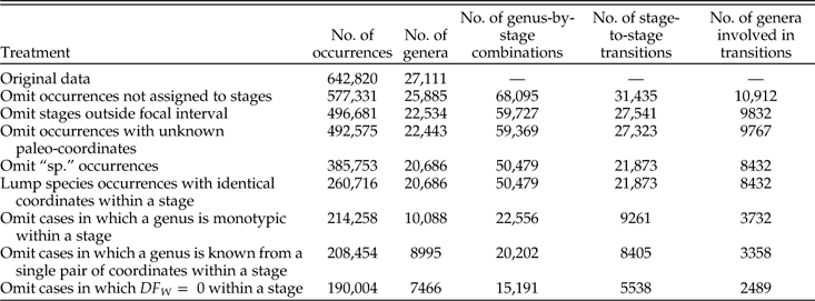
Because we are interested in the relationship between genus- and species-level geographic ranges, we need to deal with occurrences in which the species field equals “sp.” or “spp.” Although such occurrences meaningfully contribute to genus ranges, there is no rational way to assign them to a species, so we have simply omitted them. This protocol affects about 22% of occurrences but only 8% of genera (Table A1). For the genus-by-stage combinations included in our analyses, the geographic ranges of genera with and without “sp.” occurrences are well correlated; Spearman rank-order correlation coefficients are equal to 0.91 and 0.92, respectively, for the two measures of genus range (GCD gen and MS T; see below) (p ≪ 0.001 in both instances).
Using stratigraphic information in the collection records, we assigned occurrences to stratigraphic intervals, mainly international stages but also some series-level bins, that are generally more finely resolved than the standard “11-million-year’’ intervals often used in analyses of the Database. For the sake of simplicity, we will refer to operational time intervals as stages. We removed data that could not be resolved to a single stage. In contrast to our previous studies of these data (e.g., Foote and Miller Reference Foote and Miller2013; Foote Reference Foote2014), in which we used the British standard Ordovician series (Fortey et al. Reference Fortey, Harper, Ingham, Owen and Rushton1995), we assigned occurrences to the “new” international stages of the Ordovician (Gradstein et al. Reference Gradstein, Ogg, Schmitz and Ogg2012). We also subdivided the Norian and Rhaetian stages, which we had previously combined into a single interval. Our conclusions are not sensitive to these details of stratigraphic protocol. Because of data limitations that affect our ability to resolve stratigraphic occurrences in the Cambrian and to track survivorship of Pliocene and Pleistocene genera (Foote and Miller Reference Foote and Miller2013), we have focused on the Ordovician through Miocene for analyses involving ranges within single time intervals; for analyses of changes from one interval to the next, we include changes from Late Cambrian (Furongian) to the Tremadoc through those from the middle Miocene to the late Miocene.
For each occurrence we kept track of the genus, species, time interval, paleo-latitude and -longitude, and present-day latitude and longitude, the paleo-coordinates being based on the rotations of C. Scotese (personal communication to the Paleobiology Database 2001). We excluded a tiny number of occurrences lacking information on paleo-coordinates. One of our measures of geographic range is based on mean distances among coeval occurrences. Because this is potentially skewed by multiple occurrences with the same coordinates—for example, if a species is reported from several beds in a single section—we have lumped all occurrences of the same species with the same coordinates in the same time interval, as if they constituted a single occurrence for the purposes of the present analyses. This protocol affects about one-third of occurrences (Table A1); results are similar if we do not lump occurrences (Fig. A2). Because genera tend to be confined to single paleocontinents, we obtain compatible results if we use modern coordinates rather than paleo-coordinates, and we present only the results for paleo-coordinates. The concordance in results between modern and ancient coordinates also implies that our results are likely to be insensitive to alternative paleogeographic reconstructions. Because paleocontinental configurations change relatively slowly, the temporal changes in geographic range that we document should be dominated by the actual dynamics of genera rather than plate motions. Below we consider the possible effects of the geographic extent of data on apparent range dynamics.
Genus Geographic Range Size and its Components
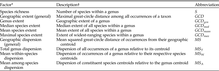
For each genus in a given stage, we used two approaches to measuring the range size of the genus and assessing the factors that contribute to it (Table 1). First, we measured range size as the maximal great-circle distance among all occurrences of the genus (GCD gen). We also calculated the range sizes of each constituent species in the same way and calculated median of the species ranges (GCD med), mean of the species ranges (GCD mean), and maximum of the species ranges (GCD max). We will refer to measures reflecting maximal great-circle distance as geographic extent.
Principal factors concerning geographic range as considered in this study.

* All factors are measured for occurrences within a single stage.
† See text for quantitative definition.
Second, by analogy to the analysis of variance, in which squared deviations from an overall mean value are partitioned into within-group and among-group components, we tabulated the distances among occurrences within a genus and partitioned them into within-species and among-species components. We will refer to measures reflecting mean squared distances as geographic dispersion.
The calculation of geographic dispersion works as follows. For each genus in each stage: S is the number of species in the genus; n i is the number of occurrences in species i; N is the total number of occurrences in the genus, equal to ∑in i; d ij is the distance from occurrence j of species i to the centroid of that species; D ij is the distance from occurrence j of species i to the centroid of the genus; and D i∙ is the distance from the centroid of species i to the centroid of the genus. (See the next paragraph for an explanation of what we mean by the centroid.) All distances are measured along great circles. We then calculate the following sums of squared distances: (1) total sum of squares, SS T, equal to ∑i∑jD 2ij; (2) within-species sum of squares, SS W, equal to ∑i∑jd 2ij; and (3) among-species sum of squares, SS A, equal to ∑in iD 2i∙. From these sums we calculate the following mean squares: (1) mean total dispersion of the genus, MS T, equal to SS T/(N−1); (2) mean within-species dispersion, MS W, equal to SS W/∑i(n i−1); and (3) mean among-species dispersion, MS A, equal to SS A/(S−1), where the quantities (N−1), ∑i(n i−1) (which equals N−S), and (S−1) are the corresponding degrees of freedom (DF T, DF W, and DF A).
We calculated the center of mass of a set of occurrences in spherical coordinates using the mean directional vector and the corresponding mean radius (R. Fisher Reference Fisher1953; N. Fisher et al. Reference Fisher, Lewis and Embleton1987: pp. 29–32). Because this center falls within the Earth itself, we found it more meaningful to project the vector to the surface and to measure great-circle distances relative to this projected mean location, which we will hereinafter refer to as the centroid. As a check on our approach, we also fitted a Fisher distribution to the occurrences of each genus in each time interval, and obtained the concentration parameter, κ (R. Fisher Reference Fisher1953). This parameter is strongly correlated with MS T (Fig. 1; Spearman rank-order correlation coefficient: r s = −0.995). (Figure 1 shows that estimated values of κ have a greater proportional spread when κ is very low, i.e., when occurrences are highly dispersed. By estimating κ from simulated data, we have verified that this feature is an expected property of the Fisher distribution. For simulation procedure, see N. Fisher et al. (Reference Fisher, Lewis and Embleton1987: p. 59.) If we were to calculate distances with respect to the actual center of mass of each genus and each species, then SS T for a genus would necessarily be exactly equal to SS W+SS A. According to our approach, SS T ≅ SS W+SS A in most cases, the greatest distortion generally occurring, as expected, when the dispersion among occurrences—and thus the difference between the actual center of mass and its projection to the surface—is greatest. If we consider the proportional deviation, (SS T−SS W−SS A)/SS T, we find that 78.4% of these deviations have a magnitude less than 0.001, and that 95% of the deviations, excluding 2.5% in each tail, fall between −0.034 and 0.0087 (Fig. 2). Thus the distortion occasionally introduced by our method of calculating centroids is negligible. In principle, if occurrences were uniformly dispersed around the globe, the mean radius could be equal to zero, i.e., the centroid could be at the center of the Earth. In practice this possibility is negligible. The smallest mean radius in our data is 0.039 (where a radius of 1.0 is at Earth’s surface), 99% of radii exceed 0.33, 95% exceed 0.52, 90% exceed 0.63, and the median is 0.95.
Comparison between geographic dispersion (per genus per time interval) as measured herein and the estimated concentration parameter of the Fisher distribution, obtained by solving numerically for κ in the equation coth(κ)−1/κ=R, where R is the mean resultant length of all the position vectors (0 ≤R ≤1, and R=1 is the radius of the Earth; see R. Fisher Reference Fisher1953 and N. Fisher et al. Reference Fisher, Lewis and Embleton1987: pp. 29–32). Because of limits on machine precision, the maximum value of κ that can be accommodated by the foregoing expression is ~710.5, corresponding to R≅0.986; we therefore omitted from this plot 3207 points with R>0.986 and κ>710.5. Dispersion and concentration are highly correlated in these data (r s=−0.995).
Cumulative frequency distribution of error in the additive partitioning of total sum of squared distances within a genus into within-species and among-species components, expressed as the proportional deviation (SS T−SS W−SS A)/SS T. 2.5% of deviations fall below the shaded area and 2.5% above it. There are 101 observations (0.66% of the distribution) that fall below the plotted limit of −0.1, and 5 observations (0.033%) that fall above 0.1. For most cases, the sum of squares can be partitioned with negligible error.
Because SS A is weighted by the number of occurrences within each species, the relative contribution of among- relative to within-species dispersion will tend to increase with increasing sampling within species. We therefore also considered an alternative measure of among-species dispersion, namely the unweighted variance among the species centroids, V A, equal to ∑iD 2i∙/(S−1). For the data studied here, MS A and V A are strongly correlated (r s=0.988), and we will present results only for MS A, but we have verified that results are consistent if we use V A instead.
Geographic extent and measures like it are commonly used in paleobiology (e.g., Hansen Reference Hansen1980; Jablonski Reference Jablonski1986, Reference Jablonski1987; Kiessling and Aberhan Reference Kiessling and Aberhan2007; Powell Reference Powell2007a,Reference Powellb; Roy et al. Reference Roy, Hunt, Jablonski, Krug and Valentine2009; Foote and Miller Reference Foote and Miller2013). With this measure, a species range size can be no larger than that of its parent genus, so GCD gen ≥ GCD med, GCD gen ≥ GCD mean, and GCD gen ≥ GCD max. No such constraint holds with respect to geographic dispersion, in which each of the quantities MS T, MS W, and MS A can be greater than, less than, or equal to any of the others. Because of the forced correlations among genus- and species-level ranges, the analyses of geographic extent that we present must be interpreted with caution. Because dispersion measures are not constrained, we suspect that the characterization of range sizes via mean dispersion will ultimately prove more useful, and we emphasize this measure of range in our interpretations. By focusing on mean rather than maximal distances, dispersion may also be less sensitive to sampled extremes (Gaston et al. Reference Gaston, Quinn, Wood and Arnold1996); the difference is akin to that between the range of variation and the variance for a random sample from a univariate distribution. Another argument in favor of dispersion is that, via the MS A term, it takes into consideration not only the number of species and their range sizes but also their locations. Moreover, although we restrict ourselves to species within genera in this paper, the analysis of dispersion allows nested designs such as species within genera within families. Despite our preference for measures of dispersion that allow the hierarchical decomposition of ranges, in the data analyzed here GCD gen and MS T are strongly correlated (product-moment r=0.81; r s=0.96), as are GCD max and MS W (product-moment r=0.74; r s=0.98).
Additional Restrictions on Data Used
Among-species dispersion cannot be measured for monotypic genera, so we omit instances in which a genus consists of a single species in a time interval. Though such instances can be included in analyses of genus extent, we favor excluding them to avoid forced redundancy between species and genus ranges (we nonetheless explore the effects of relaxing this condition for genus extent). We also omit cases in which the genus, irrespective of its species richness, is known from a single locality in a given time interval, i.e., GCD gen=0. Finally, to allow computation of MS W, we omit cases in which DF W=0, i.e., in which all species of a genus within a time interval are known from single localities. To allow comparison among results, we apply these conditions to analyses of both geographic extent and geographic dispersion.
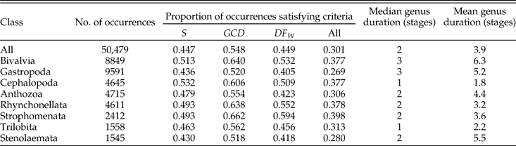
After applying the protocols described above, we are left with a total of 15,191 instances in which a genus is sampled in an included stage and meets all conditions regarding species richness, minimal range, and minimal number of within-species occurrences; and 5538 instances in which a genus meets the conditions in two successive stages. The corresponding numbers of genera included are 7466 and 2489. Table A1 gives tallies of total occurrences, genera, genus-by-stage combinations, and stage-to-stage transitions resulting from successive steps in our protocol. Fig. A1 shows how the tallies break down by class. The eight largest classes account for ~84% of the occurrences in the restricted data, and in general the proportions by class agree if we compare the raw data to the restricted data (Fig. A1A,B) or the genus-by-stage combinations to the stage-to-stage changes (Fig. A1C). For groups that are conspicuously overrepresented in the restricted data (bivalves, cephalopods, and brachiopods), this fact cannot be attributed to any single aspect of their distribution alone; inspection of the data indicates that they are above average in the proportion of instances in which genera attain our threshold in each of the three main criteria: species richness (S), GCD gen, and DF W (Table A2). Likewise, gastropods, which are underrepresented, are below average in each of the three criteria. Bivalves and cephalopods have higher and lower representation, respectively, in stage-to-stage changes than in genus-by-stage occurrences (Fig. A1C). These deviations are expected in light of the relatively long and short durations of genera in these two classes (Table A2).
Dynamics of Geographic Range
For each instance in which a genus is sampled in two successive time intervals and satisfies conditions for both, we calculated the changes in variates, namely ∆GCD gen, ∆GCD med, ∆GCD mean, ∆GCD max, ∆MS T, ∆MS W, ∆MS A, and ∆S. To analyze these changes, we first treated them as binary variables (decrease versus increase), omitting cases in which the variable did not change; most of these non-changes were in S. Omitting such cases does not affect our conclusions, as results are compatible when they are included; see Figs. 8 and 9B. We used simple and multiple logistic regression to assess the extent to which the sign of ∆GCD med, ∆GCD mean, ∆GCD max, and ∆S could predict the sign of ∆GCD gen, and likewise for ∆MS W, ∆MS A, and ∆S vis-à-vis ∆MS T.
We then used multiple linear regression to assess the extent to which the magnitude of changes in predictor variables could account for the magnitude of change in genus range size. We would like to be able to compare regression coefficients to determine, for example, whether change in number of species is a stronger or weaker predictor of genus range size than is the maximum species range. This goal is complicated by the fact that the variables are measured on different scales and have different distributions. We therefore used quantile normalization so that changes in each variable are identically distributed (see Foote and Miller Reference Foote and Miller2013). This procedure is explained in more detail below, when we present results.
Comparison Between Variation Among Coeval Genera and Temporal Variation within Genera
Because the variation in range size among coeval genera is the result of dynamic evolutionary and ecological processes, it is of interest to know how this variation relates to temporal changes within individual genera. We therefore carried out multiple regression of GCD gen on GCD max and S, rather than changes in these quantities, and likewise for multiple regression of MS T on MS W, MS A, and S. We compared the effect sizes of the predictor variables to those obtained from multiple regression analysis of the aggregate data on the changes in these quantities, not converted to binary or quantile-normalized variates.
Effects of Genus Geographic Range and its Components on Extinction Risk
For each stage, we treated MS T, MS W, and MS A as predictor variables and tallied whether each genus survived to the subsequent stage. We then carried out simple and multiple logistic regressions with survival as the response variable and compared the fit of alternative models with different sets of predictor variables via the corrected Akaike Information Criterion (AICc) and corresponding Akaike weights (Burnham and Anderson Reference Burnham and Anderson2002). The principal goal was to determine whether, once the geographic range of a genus (MS T) is specified, the way that range is partitioned (MS W and MS A) affects genus survival. Note that some models cannot be accurately estimated for some stages, because of sparse data and/or linear separation (Albert and Anderson Reference Albert and Anderson1984; Gelman et al. Reference Gelman, Jakulin, Pittau and Su2008). All results regarding survival models, whether for individual stages or for data aggregated across stages, involve only the 62 stages, out of 72 total, for which all models can be estimated.
All analyses were carried out in R, version 2.14.1 (R Development Core Team 2011). See Supplementary Table 1 for data.
Results
Dynamics of Geographic Range
Figures 3 and 4 show one example of a change in geographic range, in the bivalve genus Pteria during the Early Triassic. In the Induan stage, this genus consists of four species: one (P. ussurica) with 22 occurrences; one (P. hechuanensis) with two occurrences; and two (P. bisincilis and P. murchisoni) with one occurrence each. The three restricted species are all located near the genus centroid, which essentially coincides with that of P. ussurica (compare Figs. 3B and 3C), and the total dispersion of the genus is dominated by within-species dispersion. The geographic extent of the genus (GCD gen) is ~9800 km, the same as that of the most widely ranging species (P. ussurica), and the median and mean species extent are ~110 and ~2500 km, respectively. Two species (P. ussurica and P. murchisoni) persist into the Olenekian, accounting for four and eight occurrences, respectively, in that stage (Fig. 4). Species richness decreases by two. The total dispersion of the genus increases, as does the among-species dispersion, while the within-species dispersion decreases. The dispersion of the genus is now dominated by the among-species term. The extent of the genus decreases to ~7000 km, median species extent increases to ~2800 km, the mean species extent is nearly unchanged at ~2800 km, and the maximum species extent decreases to ~4800 km. The most wide-ranging species is now P. murchisoni rather than P. ussurica.
Geographic distribution of the bivalve genus Pteria during the Induan stage. A, All occurrences plotted on a paleogeographic map; box shows area detailed in B–D. B, Distances from occurrences to genus centroid (open black square). Magenta circles: P. ussurica; green triangle: P. bisincilis; blue diamond: P. murchisoni; red inverted triangles: P. hechuanensis. Inset magnifies region in vicinity of genus centroid. C, Distances from occurrences to species centroids (larger symbols). D, Distances from species centroids to genus centroid. See text for further discussion. Values reported for MS T, MS W, and MS A are mean squared distances.
Geographic distribution of the bivalve genus Pteria during the Olenekian stage. Colors and symbols as in Fig. 3. See text for further discussion.
For all 5538 stage-to-stage changes included in our analyses, Figure 5 shows results of a series of logistic regression models in which ∆GCD gen (negative or positive) is the response variable. The regression coefficient expresses the log odds ratio for increase in GCD gen when the predictor variable increases versus when it decreases. For example, the coefficient for mean species range is equal to 0.74 (Fig. 5B, solid square), meaning that the odds of increase in GCD gen are exp(0.74)=2.1 times higher when GCD mean increases than when it decreases.
Parameter estimates for logistic regression models relating change in genus extent (decrease versus increase) to change in predictor variable(s) (also decrease versus increase). Closed squares, our standard analysis in which a genus must have at least two species in each of two successive stages for its change in range to be included; open circles, a more relaxed analysis in which changes to or from one species are allowed; open diamonds, a more stringent analysis in which a genus must be represented by at least three species in a stage to be included. For each variable, instances in which it does not change were omitted. Because the number of cases omitted varies among models, models cannot be explicitly compared with information criteria. Change in maximum species extent (C) has a stronger effect on change in genus extent than does change in the median (A) or mean (B) species extent. Change in species richness (D) has a stronger effect still. The geographic spread of the data, measured as the number of equal-area (~2×10⁵ km2) cells containing data for a given stage, matters as well (E), but its effect is relatively weak.
We see that change in median species range size is not a strong predictor of change in genus range size (Fig. 5A). This stands to reason, given that range size distributions tend to be highly skewed, with many small ranges and a few large ones. Change in mean species range size, which is influenced by the larger part of the range-size distribution, is a much better predictor of change in genus range (Fig. 5B). Change in maximum range is a better predictor still (Fig. 5C). The role of species extent may well be exaggerated, however, because, as discussed above, the geographic extent of a genus can be no smaller than that of its widest-ranging species.
The maximum may be influenced by the number of species in the genus. If we include change in both maximum species extent and number of species in a multiple logistic regression (Fig. 5D), we see that the coefficient for the maximum declines somewhat relative to the simple regression (Fig. 5C), and that species richness is a stronger predictor than maximum extent. Genus ranges, species ranges, and number of species are all potentially influenced by the actual geographic distribution of outcrop as well as how it is sampled. We therefore divided the globe into a 50×50 equal-area grid after carrying out a Lambert cylindrical projection, and we tabulated the geographic extent of available data, measured as the number of equal-area (~2×10⁵ km2) cells containing data for a given stage, and included it in the regression (Fig. 5E). Although change in sampled area has a noticeable effect on changes in genus extent, this effect is swamped by the effects of maximum species extent and species richness.
If we relax the condition that each genus contain at least two species per stage, the regression coefficients for species extent and species richness all increase by a comparable amount (Fig. 5), implying that transitions to or from monotypic status are an important element of the dynamics of genus range size, at least when measured as geographic extent. Changing the species threshold from two to three has a smaller effect than changing it from two to one (Fig. 5; see also Figs. 8 and 9).
In light of the relative magnitudes of regression coefficients, we will hereinafter restrict analyses to those involving GCD max and will no longer consider GCD med or GCD mean.
Because species richness takes on integer values, whereas changes in genus and species range sizes vary continuously, we have used ∆S as a reference distribution onto which to map the other variables in carrying out quantile normalization, as noted earlier. Figure 6 shows the frequency distributions of ∆S, ∆GCD gen, and ∆GCD max. Because the distribution of ∆S has very long and sparse tails, we have combined all values ≤−6 and all values ≥6 (Fig. 7A). The left-most bar in Figure 7A accounts for 8.4% of the distribution; therefore the lowest 8.4% of the values of ∆GCD gen and ∆GCD max are assigned a value of −6. Of the values of ∆S, 2.7% are equal to −5, so the next 2.7% of the values of ∆GCD gen and ∆GCD max are assigned a value of −5, and so on. The mapping of the original values of ∆GCD gen and ∆GCD max onto their quantized equivalents is shown in Figure 7B, C. Because the tails of the respective distributions differ greatly in shape, we have omitted the lowest and highest quantiles from analysis. We carried out quantile normalization of ∆MS T, ∆MS W, and ∆MS A in the same way.
Histograms showing change in number of species within each genus (A), change in genus geographic extent (B), and change in maximal species extent for each genus (C). Because variables differ in the shapes of their distributions and the scales on which they are measured, we use quantile normalization to compare effect sizes (see Figs. 7–8).
Steps in quantile normalization of data. A, Distribution of change in species richness within each genus, comparable to Fig. 6A but with tails combined into a single value. B, Normalization of change in genus extent. The lowest 8.4% of the values are assigned to the first bin, the next 2.7% to the second bin, and so on. C, Normalization of changes in maximum species extent.
The regression of quantile-normalized variates is consistent with the logistic regression of binary variates in showing: (1) that change in species richness has a larger effect on genus extent than does change in maximum species extent; (2) that both effects are larger when transitions to and from monotypic status are included; and (3) that sampling is of secondary importance in determining genus range size (Fig. 8).
Effect sizes from multiple linear regression of quantile-normalized change in genus extent on changes in maximum species extent, species richness, and geographic spread of data; symbols as in Fig. 5. Consistent with the logistic regression of binary variables (Fig. 5E), species richness has the strongest effect on genus extent; geographic extent of the data has the weakest effect; and effects of species extent and species richness are strongest if transitions to or from monotypic status are included.
Figure 9 shows results of multiple regression of ∆MS T on ∆MS W, ∆MS A, ∆S, and changes in the geographic extent of sampled data. For both binary and quantile-normalized variates, ∆MS A has the strongest effect on ∆MS T; this is followed by ∆MS W, which, depending on the analysis, has either a larger or a comparable effect compared with ∆S. Thus, when a genus expands or contracts its geographic range—measured as MS T—this change is attributable much more to the placement of its constituent species than by their internal dispersion or the number of them. Sampling is of minor importance.
Effect sizes from multiple logistic regression of binary variables (A) and multiple linear regression of quantile-normalized variables (B) relevant to changes in genus geographic dispersion (MS T). Symbols as in Fig. 5. Among-species dispersion (MS A) has the strongest effect on genus range. Within-species dispersion (MS W) has an effect either distinctly stronger than (A) or comparable to (B) that of species richness. The effect of geographic spread in the data is relatively minor.
Comparison Between Variation among Coeval Genera and Temporal Variation within Genera
Analyses of coeval genera and of changes within individual genera are compared in Tables 2 and 3. The effect sizes estimated from the static and dynamic regressions are remarkably similar. Each km change in the maximal species extent (GCD max) corresponds to a change of between ~0.4 and ~0.6 km in the genus extent (GCD gen). Adding or subtracting a species yields an average change of between ~200 and ~300 km in GCD gen. These results imply that a change of one species has the same effect as a change of ~500 km in GCD max.
Contributions to genus extent (GCD gen): multiple linear regressions for static (variation among coeval genera) vs. dynamic (stage-to-stage variation within genera) relationships.

Contributions to genus dispersion (MS T): multiple linear regressions for static (variation among coeval genera) vs. dynamic (stage-to-stage variation within genera) relationships.
Each unit change in within-species dispersion (MS W ) or in among-species dispersion (MS A) yields roughly one-half or one-quarter of a unit response, respectively, in total genus dispersion (MS T) (Table 3). Note that the relative magnitudes of the regression coefficients in Tables 2 and 3 should not be interpreted in terms of the relative importance of the predictors, because the distributions of the variates differ substantially. For example, MS A has a much higher variance than does MS W (2.9×10¹⁵ km4 versus 1.1×10¹⁴ km4), and the median absolute change in MS A is also much higher than that of MS W (1.9×10⁷ km2 versus 6.3×10⁵ km2). Thus, even similar regression coefficients would imply a larger impact of MS A versus MS W, consistent with Figure 9.
Effects of Genus Geographic Range and its Components on Extinction Risk
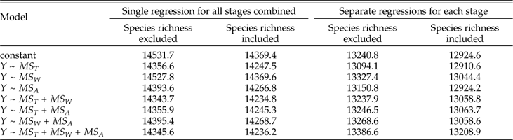
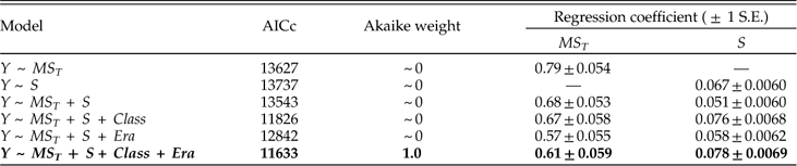
We present the full suite of additive models in Table A3, but focus here on just a few key comparisons. First, do we obtain a better model fit, assessed via AICc, by aggregating data from all stages and fitting a single regression relationship, or by fitting separate regression coefficients for each stage? Regardless of which set of predictors we consider, the fit is substantially better if we allow regression coefficients to vary among stages, with ∆AICc values from ~960 to ~1300. From here forward we will therefore focus on survival models that allow variation among stages. Second, once the geographic range of a genus is specified, does adding data on how it is structured improve the model fit? Evidently not; models including MS T alone as a predictor of survival all fit substantially better than corresponding models that also include MS W and/or MS A, with ∆AICc values ranging from ~140 to ~290. Given the strong correlation between MS T and MS A (product-moment r=0.79; r s=0.96), it is also noteworthy that the model including MS T alone provides a better fit than that including MS A alone (∆AICc=57). Finally, once geographic range and its components are specified, does species richness provide additional predictive power? Evidently so; for every model we obtain a better fit by including species richness as a predictor of genus survival. Of all sixteen possible combinations of predictors, the best fitting model includes just MS T and S. Thus, just as adding species richness to a model with genus dispersion as the only predictor of survival improves the fit, so too does adding genus dispersion to a model with species richness as the only predictor (Table A3). The simplicity of the best-fitting model gives some confidence that our results do not reflect model overfitting (Burnham and Anderson Reference Burnham and Anderson2002).
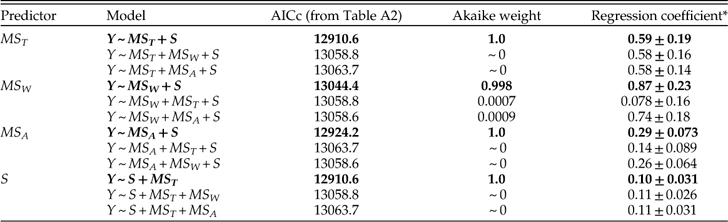
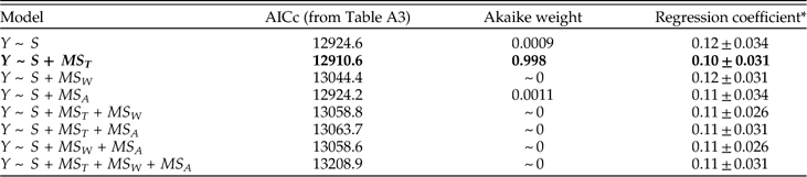
In assessing alternative models of survival, we should consider not only the model fit but also the regression coefficients. For each predictor variable, Table 4 presents coefficients for the best-fitting model including that predictor, as well as two alternative models with the other predictors included in turn. (Because S consistently improves model fit, this variable is included as a predictor in all models.) Regardless of the model, we see that MS T is a good predictor of survival. MS W also predicts survival if it is considered by itself or with MS A. But adding MS W to a model that already includes MS T results in regression coefficients that do not differ appreciably from zero. The change in regression coefficient suggests that the apparent effect of MS W on survival in a simple regression model may reflect its correlation with MS T, and it complements the earlier finding that adding MS W does not improve model fit once MS T is known. Similarly, if MS A is considered alone or with MS W, it predicts survival, but this predictive power is diminished—albeit not quite to oblivion—when the model includes MS T. Species richness, S, also consistently predicts genus survival, irrespective of the model. In particular, all else being equal, each additional species increases the odds of survival by a factor of roughly 1.1.
Coefficients of MS T, MS W, MS A, and S in logistic regression models of genus survival. Y denotes whether a genus does (1) or does not (0) survive beyond the stage of observation. Models are fit separately for each of 62 stages. For each predictor, best-fitting model including that predictor (highlighted in boldface) is compared with models that also include each of the other two predictors respectively. In this and subsequent tables depicting survival models, dispersion is measured as square radians.
* Median of stage-level coefficients ± one standard error, based on bootstrap resampling.
Discussion
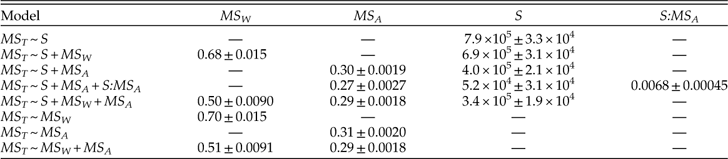
Our results suggest that species richness is more important than the geographic ranges of individual species in determining geographic extent of genera, consistent with what has been found for living bivalves (Roy et al. Reference Roy, Hunt, Jablonski, Krug and Valentine2009), whereas geographic dispersion of genera is dominated primarily by the dispersion among species and only secondarily by within-species dispersion and species richness. Moreover, species richness seems to be more important in determining dynamic changes in genus extent than in genus dispersion, not only in relative terms but also in absolute terms, as we can see by comparing the regression coefficients in Figures 5, 8, and 9. We can gain some insight into the role of species richness by considering a series of models in which it is considered as a predictor of genus dispersion on its own and in combination with the within- and among-species components of dispersion (Table 5). The regression coefficient for species richness drops roughly in half when among-species dispersion is included in the model, suggesting that the tacit assumption that these factors act independently—i.e., additively—is violated. Indeed, when we add an interaction between species richness and among-species dispersion in the model, the model fits much better (∆AICc=228), this interaction term is significant (albeit comparatively weak, accounting for 7.8% of predicted genus dispersion on average), and the effect of species richness drops by an order of magnitude and no longer differs significantly from zero (p=0.094). This result evidently does not simply reflect a collinearity between MS A and S; the product-moment and rank-order correlations between them are equal to only 0.12 and 0.33, respectively. Genera with greater among-species dispersion clearly tend to be more widespread in any event, but the added impact of species richness is principally felt in those genera that have more species and greater dispersion among them. In contrast to species richness, the estimated effects of within- and among-species dispersion on genus dispersion vary relatively little among alternative models (Table 5).
Coefficients of MS W, MS A, and S for alternative models predicting genus dispersion (MS T). These results show regression coefficients (± 1 S. E.) for variation among coeval genera. S:MS A denotes an interaction.
One might suspect that the minor importance of species richness in the dynamics of geographic dispersion could be an artifact of the uncertainty with which the number of species, in contrast to the locations of occurrences, is known, especially in light of our need to remove “sp.” occurrences. If this were the case, however, we would also expect regressions involving geographic extent and survival to show a small role for species richness, which is not what we see (Figs. 5, 8; Tables 4, A4).
Another indication that species richness is not a major factor in determining the dynamics of genus dispersion comes from an analysis wherein we separately consider instances in which genus dispersion decreases and those in which it increases (Table 6). MS W and MS A have comparable effects for expanding and contracting genera, but the effect of species richness is negligible. The effect of species richness when expanding and contracting genera are combined (Table 3; Fig. 9) reflects a regression through a cluster of contracting genera that decrease in species richness and a cluster of expanding genera that increase in species richness, with virtually no relationship between the magnitude of ∆S and of ∆MS T within either cluster.
Multiple regression of change in genus dispersion (∆MS T) on ∆MS W, ∆MS A, and ∆S, analyzed separately for cases in which ∆MS T < 0 and ∆MS T > 0. Compare with Table 3.
The symmetry between expanding and contracting genera suggests a model of genus dispersion dynamics in which genera expand/contract via both the increase/decrease in dispersion of individual species and the shift of species away from/toward the center of the genus range, but not by a net increase/decrease in the number of species. This model is similar to that of Krug et al. (Reference Krug, Jablonski and Valentine2008) for Cenozoic bivalves, whereby genera expand from their region of origin via a “moving front” of species, although it differs in considering range contraction as well as expansion.
The limited role of species richness in the dynamics of genus dispersion naturally raises the question of whether the apparent effect of species richness on genus survival (Table 4) could in fact reflect a collinearity with geographic dispersion that prevents us from estimating additive effects of these factors accurately (Finnegan et al. Reference Finnegan, Payne and Wang2008). The stability of the effect of species richness across a wide range of survivorship models (Tables 4, A4) suggests that this is not the case. Moreover, the correlation between species richness and genus dispersion is not very strong (product-moment r=0.19; r s=0.35). Given these results and the consistent improvement in model fit when species richness is added as a predictor to survivorship models (Table A3), we infer that species richness in its own right has a direct effect on the survival of genera, beyond its contribution to geographic range. Because this effect transcends that of geographic range, a reasonable hypothesis is that species richness reflects ecological diversity and that such diversity in turn buffers a genus against extinction (see Kolbe et al. Reference Kolbe, Lockwood and Hunt2011). However, it is also possible that the species is in effect the basic unit of extinction, so that greater species richness, through “strength in numbers,” buffers a genus even if does not reflect greater ecological diversity.
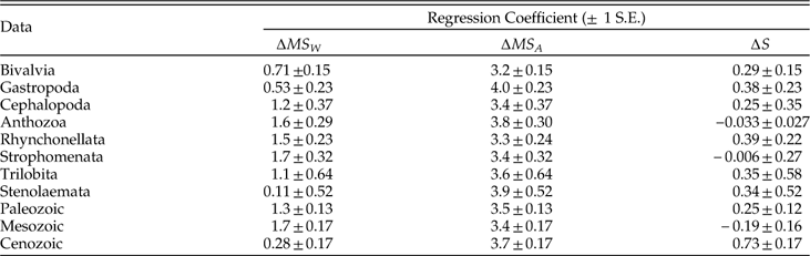
We have largely ignored temporal and taxonomic heterogeneity in our analyses (but see Table A2). To explore the effects of this variation, we have focused on the eight largest classes, accounting for 83.8% of the genus-by-stage occurrences, and have added class membership and era of occurrence as factors in regression models. As one example, Table A5 shows that adding class and/or era does not substantially improve our ability to predict the direction of change in dispersion within a genus from one stage to the next. Because genera have about as many instances of expansion as contraction in their lifetimes (51% expansions and 49% contractions in the aggregate data analyzed here), this result stands to reason. However, it leaves open a rather different question: whether the dynamics of geographic range, i.e., the details of how changes in genus dispersion relate to the components of dispersion, vary over time or among classes. If we model the dynamics separately by class and era, we see that the regression coefficients vary in magnitude, and that those for ∆MS W and ∆S do not always differ appreciably from zero (Table A6). The reasons for these differences are beyond our scope. However, the differences are overshadowed by the result that among-species dispersion (∆ MS A) is consistently the most important predictor of whether a genus expands or contracts.
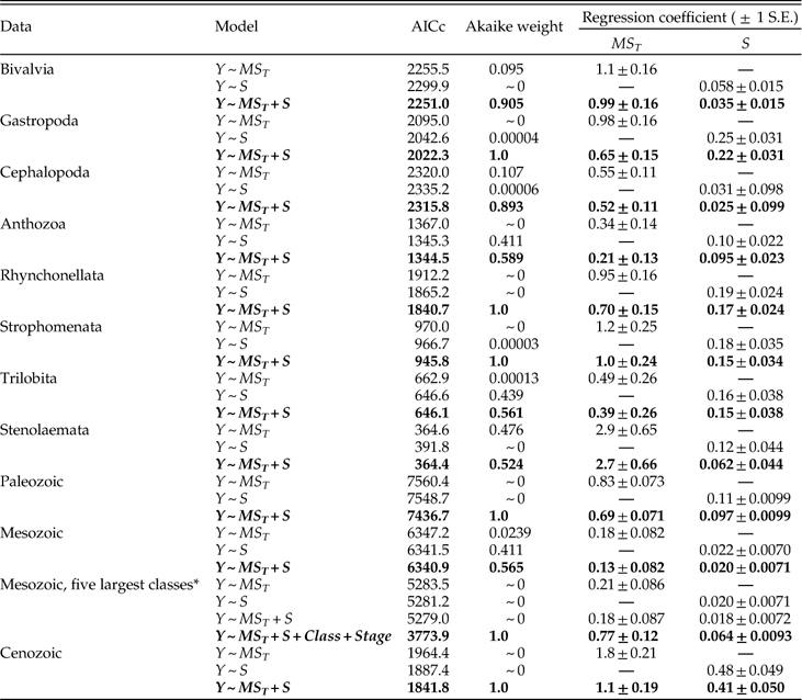
We carried out similar analyses for models of genus survival. Because some taxonomic subsets of data are too small to allow stage-by-stage analysis, we have aggregated data for each subset into a single analysis, combining all 72 stages (cf. Table 4). Adding information on class and era substantially improves our ability to predict genus survival (Table A7). This result is as expected, in light of the well-known secular decline in extinction rate (Raup and Sepkoski Reference Raup and Sepkoski1982; Van Valen Reference Van Valen1984; Sepkoski Reference Sepkoski1986; Benton Reference Benton1995) and among-group differences in extinction rate (Simpson Reference Simpson1953; Stanley Reference Stanley1979, Reference Stanley1985; Raup and Boyajian Reference Raup and Boyajian1988). Again, a separate question is whether the details of the survival models differ among taxa and over time. Comparing models that predict survival as a function of MS T, S, or both, we find that the model including both predictors fits best for every subset of data (Table A8), although the preference for this model is weak in corals, trilobites, and stenolaemate bryozoans, and during the Mesozoic. Thus, one of our principal results, that species richness enhances survival beyond its effect on geographic range, is a fairly general feature. The strength of selectivity, however, varies considerably among classes and over time. A conspicuous case concerns weak selectivity during the Mesozoic, which we have documented previously (Foote and Miller Reference Foote and Miller2013). Dissection of Mesozoic selectivity will be the subject of a forthcoming contribution; for now we will simply mention that, when class and stage (as an unordered factor) are taken into consideration, we see clear selectivity of genus survival with respect to geographic range and species richness (Table A8).
Our findings regarding the role of species richness in genus survival contrast with those of Finnegan et al. (Reference Finnegan, Payne and Wang2008), who concluded that it adds relatively little predictive power once geographic range is taken into account. There are too many differences in data treatment to allow us to pinpoint the precise reasons for the discrepancy, but we suggest that their measure of geographic range (occupancy of 10° by 10° grid cells) is an important factor, for such measures tend to be rather well correlated with species richness. If we recompute genus geographic range as the number of occupied equal-area cells (~8×10⁵ km2, approximately the same size as 10° by 10° cells on average), richness has a substantially stronger correlation with this measure (r s=0.63) than with dispersion (r s=0.35, as noted above). In hindsight, we see the relatively low correlation with species richness as another advantage of using dispersion to measure geographic range.
Genus geographic dispersion unambiguously predicts survival, whereas its components, within- and among-species dispersion, have comparatively little effect once genus dispersion is taken into account (Table 4). This result provides support for the general notion that it is the emergent properties of the genus that determine its evolutionary fate, and that these are to a large extent screened off from the underlying properties that give rise to them (Jablonski Reference Jablonski2008). When it comes to survival, it is of primary importance how widespread a genus is, and not whether it achieves its range through component species ranges that are themselves broad versus narrow, close together or far apart. This mirrors the finding that survival of molluscan genera through the end-Cretaceous extinction event depended on geographic ranges of genera rather than the ranges of their constituent species (Jablonski Reference Jablonski1986), but it generalizes the result beyond this extreme event. The overarching dominance of this genus-level property emphasizes the importance of hierarchical approaches to studying evolution and stands in contrast to a recent suggestion that genus-level patterns are ephiphenomenal (Hendricks et al. Reference Hendricks, Saupe, Myers, Hermsen and Allmon2014).
The similarity in effect sizes when we compare among-genus variation at a point in time to variation within genera over time suggests that a static cross-section provides a reasonable approximation of a dynamic process. Such a result is not a foregone conclusion. For example, cross-sectional variation in biometric traits within a population does not necessarily provide a clear reflection of longitudinal variation (Cock Reference Cock1966). Nonetheless, the symmetry in determinants of expansion and contraction seen at the time scale of single stages (Table 6), much like the roughly symmetrical pattern of waxing and waning seen over longer spans of time within genera and species (Jernvall and Fortelius Reference Jernvall and Fortelius2004; Raia et al. Reference Raia, Meloro, Loy and Barbera2006; Foote Reference Foote2007, Reference Foote2014; Foote et al. Reference Foote, Crampton, Beu, Marshall, Cooper, Maxwell and Matcham2007, Reference Foote, Crampton, Beu and Cooper2008; Liow and Stenseth Reference Liow and Stenseth2007; Liow et al. Reference Liow, Skaug, Ergon and Schweder2010; Tietje and Kiessling Reference Tietje and Kiessling2013; cf. Nicol Reference Nicol1954) suggests limitations to what we can infer from a static comparison of ranges among genera. In particular, it would not be evident without a dynamic analysis whether some genera are more narrowly distributed than others because they have expanded less or contracted more than others. Are they on their way up or on their way down? This same point applies in other fields as well. For example, we would be hard-pressed to know, without a historical record, whether a bit of internet slang such as lol, wt[h], or iirc is at low frequency because it is new and starting to expand; because it was once popular but is on the wane; or because it never caught on for intrinsically maladaptive reasons (Altmann et al. Reference Altmann, Pierrehumbert and Motter2011). It stands to reason that attempts to infer the dynamics of geographic range from present-day ranges alone, without reference to the fossil record, have led to a mixed bag of interpretations (Gaston Reference Gaston1998, Reference Gaston2008).
Conclusions
1. Although species richness is an important predictor of the dynamics of maximal geographic extent of a genus, it affects the dynamics of genus geographic dispersion relatively little.
2. The mean dispersion among species is the principal determinant of the dynamics of total genus dispersion, but within-species dispersion also plays an important role.
3. The contributions of within- and among-species dispersion to variation in range among coeval genera are similar to those within genera over time. Moreover, there is a distinct symmetry in how these factors shape genus range at times when genera are expanding versus contracting. In particular, genera expand and contract principally by increasing the net distances among species without necessarily changing the number of species. These results are consistent with prior work in suggesting that understanding the dynamics of geographic range requires historical analysis and is unlikely to be possible solely on the basis of a sample of living species.
4. Geographic dispersion of a genus is a clear predictor of survival from one stage to the next. Once dispersion is known, however, how it is structured by within- and among-species dispersion adds little or no predictive power. This is consistent with a hierarchical view of evolution in which the fate of an entity may depend only or mainly on properties expressed at its level of organization and may be screened off from properties at lower levels.
5. Although species richness is of secondary importance in determining the dynamics of geographic dispersion of genera, it significantly enhances the chances of genus survival above and beyond its contribution to geographic range.
Acknowledgments
We are grateful to the many people who have contributed data to the Paleobiology Database. Major contributors for the data used herein include M. Aberhan, J. Alroy, D. Bottjer, M. Carrano, M. Clapham, S. Finnegan, F. Fürsich, S. Gouwy, N. Heim, A. Hendy, S. Holland, M. Hopkins, L. Ivany, D. Jablonski, W. Kiessling, M. Kosnik, B. Kröger, A. McGowan, T. Olszewski, P. Novack-Gottshall, J. Pálfy, M. Patzkowsky, A. Stigall, M. Uhen, L. Villier, and P. Wagner. D. W. Bapst gave extensive assistance with lower Paleozoic stage assignments. C. Scotese provided the paleogeographic base maps for Figures 3 and 4. We thank W. Allmon, D. Jablonski, J. Pierrehumbert, and P. Smits for discussion; and W. Kiessling and J. Payne for thoughtful reviews and suggestions. Supported by NASA Exobiology (NNX10AQ44G). This is Paleobiology Database publication number 236.
Supplementary Material
Supplemental data archived at Dryad: doi: 10.5061/dryad.nh6hm
Appendix
Effect of vetting protocols on amount of data retained.
Proportion of genus-by-stage occurrences meeting specified criteria described in text. Also given are median and mean genus durations (number of stages) for all genera, including those not retained for analysis. Data limited to stages included in analyses.
Comparison of AICc among models predicting genus survival (Y) as a function of MS T, MS W, MS A, and S (species richness).
Regression coefficients showing effect of species richness in alternative models of genus survival (Y). See Table 4 for explanation.
Comparison of models predicting change in dispersion, with and without class and era as additional predictors. Data limited to the eight largest classes. Variates treated as binary (decrease versus increase; see Fig. 9A). Best-fitting model in boldface.
Comparison among classes and eras of model predicting change in genus dispersion (∆MS T) as a function of ∆MS W, ∆MS A, and ∆S, with variates treated as binary (decrease versus increase; see Fig. 9A).
Comparison among models predicting genus survival, with and without class and era as additional predictors. Data limited to eight largest classes and analyzed in aggregate, rather than stage-by-stage. Best-fitting model in boldface.
Comparison among selected models predicting genus survival, for subsets of data analyzed in aggregate, rather than stage-by-stage. Best-fitting models in boldface.
Proportional representation of classes in raw data and data retained for analysis, restricted to the included time intervals; class assignment could not be determined from downloaded information in 0.6% of cases. Each point denotes a class; eight classes accounting for largest proportion of analyzed data are indicated. Diagonal is the 1:1 line. A, Genus-by-stage occurrences in raw vs. analyzed data. B, Stage-to-stage transitions in raw vs. analyzed data. C, Genus-by-stage occurrences vs. stage-to-stage transitions in analyzed data. All comparisons show a positive correlation, with several classes overrepresented in analyzed data relative to raw data; these deviations reflect above average proportions of genera satisfying all three minimal criteria (for S, GCD gen, and DF W) rather than any single one (Table A2). Bivalves and cephalopods have higher and lower representation, respectively, in stage-to-stage transitions than in genus-by-stage occurrences; these deviations reflect longer and shorter genus durations, respectively.
Multiple logistic regression of changes in geographic dispersion (MS T) when occurrences of a species with the same paleo-coordinates in the same stage are not lumped. Absolute and relative effect sizes of predictors are similar to those resulting from analysis of lumped occurrences (Fig. 9).