



1 Introduction
Gravity currents are formed due to a density difference in the horizontal direction between a current and an ambient fluid (see, e.g. Simpson Reference Simpson1997; Ungarish Reference Ungarish2009). Such flows are important in many environmental, geophysical and industrial applications including dam-break problems, chemical spillage, fluid injection in porous medium (see, e.g. Huppert & Woods Reference Huppert and Woods1995; Zheng et al. Reference Zheng, Guo, Christov, Celia and Stone2015), oil spreading (Hoult Reference Hoult1972), open channel flows and stratified flows (see Maxworthy et al. Reference Maxworthy, Leilich, Simpson and Meiburg2002; Gladstone et al. Reference Gladstone, Ritchie, Sparks and Woods2004; White & Helfrich Reference White and Helfrich2008; Sher & Woods Reference Sher and Woods2015).
Schematic illustrations of (a) the dam break, (b) the spreading configuration with possible substrate drainage and (d) the edge drainage configuration for a finite-volume release of fluid. Schematic view of the geometry of the current work is shown in (c). When the right-hand wall is removed, the fluid flows over the edge. Here
 $x$
is the horizontal coordinate,
 $t$
is time,
 $h(x,t)$
is the height of the gravity current and
 $u(x,t)$
is the vertically averaged horizontal velocity of the fluid. Also,
 $\unicode[STIX]{x1D70C}_{c}$
and
 $\unicode[STIX]{x1D708}_{c}$
are, respectively, the density and kinematic viscosity of the gravity current and
 $\unicode[STIX]{x1D70C}_{a}$
and
 $\unicode[STIX]{x1D708}_{a}$
denote, respectively, the density and kinematic viscosity of the ambient fluid.

In the high Reynolds number limit for such flows, viscous effects can often be assumed to be negligible and the dominant momentum balance is between buoyancy and inertia. Huppert & Simpson (Reference Huppert and Simpson1980) found that inertial gravity currents, produced by releasing a fixed volume of fluid into another of slightly lower density over a flat wall, evolve through two states in the high Reynolds number (
 $Re$
) limit: a slumping phase and an eventual inertial self-similar phase. In a typical experiment, once the gate is removed, a portion of the fluid in the reservoir will remain stationary (see figure 1
a). This is the initial part of the slumping phase. The slumping process has been previously studied with the help of the shallow-water theory (see e.g. Hogg & Pritchard Reference Hogg and Pritchard2003; Ungarish Reference Ungarish2007; Balmforth, Hardenberg & Zammett Reference Balmforth, Hardenberg and Zammett2009; Ungarish Reference Ungarish2011). After a rarefaction wave reaches the left wall, the transition phase continues until the initial conditions of the flow are completely forgotten in the self-similar inertial flow regime. Huppert & Simpson (Reference Huppert and Simpson1980) focused on the slumping process of inertial currents in the Boussinesq approximation and argued that the Froude number (
 $Fr\equiv$
speed of fluid relative to the typical speed of gravity waves) at the leading edge increases in this phase and becomes constant in the inertial stage, analogous to the two dynamical phases of the
 $Fr$
suggested by Benjamin (Reference Benjamin1968) for spreading currents.
Inertial gravity currents are generally controlled by the front conditions and many studies have investigated the controlling conditions or
 $Fr$
at the front (see e.g. Benjamin Reference Benjamin1968; Huppert & Simpson Reference Huppert and Simpson1980; Borden & Meiburg Reference Borden and Meiburg2013). For instance, Rottman & Simpson (Reference Rottman and Simpson1983) obtained analytical solutions for currents in a Boussinesq system flowing in a rectangular channel, which is usually called the dam-break problem, as one of the early parameterizations of the spreading currents (figure 1
a). In particular, in the high
 $Re$
limit, they found that the current passes through two distinct dynamical phases: a slumping phase and an eventual inertial self-similar phase as introduced above. The non-Boussinesq gravity current problem, which involves large density differences, occurs often in nature such as in motion of avalanches, releases of dense gases and plumes into the atmosphere (Rooney & Linden Reference Rooney and Linden1996), water–air interface evolution (Wilkinson Reference Wilkinson1982; Baines, Rottman & Simpson Reference Baines, Rottman and Simpson1985) and pyroclastic flows. Despite several recent investigations (Grobelbauer, Fannelop & Britter Reference Grobelbauer, Fannelop and Britter1993; Lowe, Rottman & Linden Reference Lowe, Rottman and Linden2005; Ungarish Reference Ungarish2010; Rotunno et al.
Reference Rotunno, Klemp, Bryan and Muraki2011; Dai Reference Dai2014), the studies on non-Boussinesq cases are limited (Ungarish Reference Ungarish2011), and we focus on non-Boussinesq systems in this work.
In recent years, various extensions to the classic spreading problem have been studied with the help of analytical modelling, numerical simulations and laboratory experiments (see e.g. Ungarish Reference Ungarish and Fernando2013a
; Meiburg, Radhakrishnan & Nasr-Azadani Reference Meiburg, Radhakrishnan and Nasr-Azadani2015). For instance, Gratton & Vigo (Reference Gratton and Vigo1994) used a phase plane analysis to investigate flows on a plane with variable inflow and identified a series of self-similar solutions for inertial gravity currents. Marino, Thomas & Linden (Reference Marino, Thomas and Linden2005) examined the front boundary conditions of gravity currents, in which they found that both
 $Fr$
and
 $Re$
at the head are important. The extended inertial spreading problem has also been studied by considering non-flat bottom boundaries (Ellison & Turner Reference Ellison and Turner1959; Britter & Linden Reference Britter and Linden1980; Beghin, Hopfinger & Britter Reference Beghin, Hopfinger and Britter1981; Ross, Linden & Dalziel Reference Ross, Linden and Dalziel2002; Monaghan et al.
Reference Monaghan, Meriaux, Huppert and Monaghan2009), turbulent flow effects (Sher & Woods Reference Sher and Woods2015), axisymmetric currents (Grundy & Rottman Reference Grundy and Rottman1985; Hallworth, Huppert & Ungarish Reference Hallworth, Huppert and Ungarish2003) and substrate drainage on porous boundaries (figure 1(b), Ungarish & Huppert Reference Ungarish and Huppert2000; Thomas, Marino & Linden Reference Thomas, Marino and Linden2004) which are related to the theme of this paper.
Nevertheless, the drainage of a gravity current from an edge has received less attention (figure 1 c). The drainage from an edge poses a new boundary condition in the flow that is distinct from the boundary conditions in the dam-break or spreading configurations (front conditions). There have been some studies that parametrized the inviscid flow with an inflow in a waterfall-like configuration (e.g. Clarke Reference Clarke1964; Naghdi & Rubin Reference Naghdi and Rubin1981; Dias & Tuck Reference Dias and Tuck1991). However, the sudden release of a constant fluid volume from the edge of tanks (without any inflow) with different shapes remains an open problem. We investigate this configuration under the unconfined condition where the motion of the ambient fluid is negligible.
Previous studies on waterfall flows over an edge are under steady-state situations, in which a constant inflow is assumed at the boundary. However, in the current work, there is no inflow, and the fully unsteady problem experiences two distinct stages in the high
 $Re$
limit: an initial adjustment phase and a late-time inertial phase. Hence, characterizing the unsteady behaviour of the drainage over an edge, without inflow, frames the goal and contribution of this work. Zheng et al. (Reference Zheng, Soh, Huppert and Stone2013) have examined a similar problem for low
 $Re$
flows in a porous reservoir and a self-similar solution was obtained to describe the interface shape after an inertial phase transition. The main objective of this paper is to investigate the release of a finite volume of fluid from an edge for high
 $Re$
flows (an inertial regime), i.e.
 $Re\gtrsim 10$
. In particular, we aim to answer the following questions: What is the dynamics associated with fluid drainage from an edge of a rectangular tank? Can we capture the dynamics using a simplified analytical model and how do these results compare with experiments and direct numerical solutions?
A schematic view of our problem, and a comparison with other related problems (figure 1
a,b), is shown in figure 1(c,d). A tank, with a horizontal planar bottom and length
 $L$
, is initially filled with the fluid to height
 $h_{0}$
and a lock gate is used to contain the fluid. Then the lock gate is lifted, the fluid flows over the edge and the tank drains. We treat the problem as two-dimensional. The detailed shape of the current is
 $h(x,t)$
. We do not account for the mixing across the interface between the two fluids and we assume that the density difference between the current and the ambient fluid is large (
 $\unicode[STIX]{x1D70C}_{c}/\unicode[STIX]{x1D70C}_{a}\gtrsim 10$
where
 $\unicode[STIX]{x1D70C}_{c}$
and
 $\unicode[STIX]{x1D70C}_{a}$
are the density of the gravity current and ambient fluid respectively). Moreover, the drainage is unopposed at the edge of the flow.
In § 2 we introduce the experiments after which in § 3 we present the direct numerical simulations of the gravity current and describe the drainage dynamics. Then, in § 4 we develop a reduced-order model, which is derived from the shallow-water equations and scaling arguments. In § 5, we validate our analytical solutions and scaling arguments against experiments and direct numerical simulations. Finally, we discuss the model’s assumptions, limitations and implications in § 6.
2 Experiments
Three geometries were used to conduct twenty experiments. Here we study six of them with different
 $h_{0}$
and
 $L$
as shown in table 1. A small (cases E1 and E2), a medium (cases E3 and E4) and a large tank (cases E5 and E6) are initially filled with fresh tap water and a lock gate is used to contain the water. A small amount of cyan dye or black ink is added for better flow visualization. In each experiment, the gate was lifted rapidly and the motion of the water in the tank was filmed from the side. We varied the initial depth
 $h_{0}$
by approximately a factor of 2 and also the tank length
 $L$
by approximately a factor of 2. Figure 2 exhibits the results of the free-surface shape for case E6 at four times (see supplementary materials available at https://doi.org/10.1017/jfm.2017.480 for animations).
Details of the experiments performed for inertial gravity currents of water draining from the edge of a tank;
 $\unicode[STIX]{x1D70C}_{c}=998~\text{kg}~\text{m}^{-3}$
,
 $\unicode[STIX]{x1D70C}_{a}=1.2~\text{kg}~\text{m}^{-3}$
and
 $\unicode[STIX]{x1D708}_{c}=1.0\times 10^{-6}~\text{ m}^{2}~\text{s}^{-1}$
.

We observe from the upper part of figure 2 that after the release of the gate the fluid height initially starts decreasing very slowly near the end wall and a little faster near the right boundary (early-time behaviour). This effect occurs through a wave that propagates along the fluid interface towards the left boundary, after which all of the current is impacted by the drainage at the right boundary. Once this wave is reflected by the end wall and exits at the open right boundary, all the heights at different positions decrease with the same time dependence (late-time behaviour that we focus on here). The late-time behaviour continues up to the point where viscous effects become of the same order as the inertial effects.
The gravity current of case E6 at
 $t=0.0$
s (initial condition),
 $t=0.3$
s (early period),
 $t=0.6$
s (transition period) and
 $t=0.9$
s (late period) from (a) to (d) respectively. Red lines at the left show a scale bar of 1 cm length.

3 Direct numerical simulations
3.1 The suite of simulations
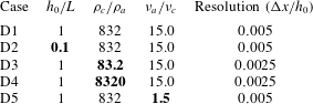
We implemented two-dimensional direct numerical simulations (DNS) with a similar set-up as in figure 1(c) using OpenFoam v2.4 (interFoam multiphase solver), which is an open-source code developed to solve the two phase fluid (gas and/or liquid) continuity and Navier–Stokes equations. The details of the code, numerical solver, mesh grid cells, domain size, governing equations, a sketch of the simulation set-up and boundary conditions are described in appendix A. Table 2 shows the details of the direct numerical simulations performed and their initial conditions. Figure 3 depicts a typical snapshot from the DNS in the late-time period of case D1 at
 $t=0.38$
s. One can compare this figure with the profiles of figure 2; it is clear that both figures exhibit similar shapes, which will be compared in detail below. Note that case D1 is our basic case in which water is the gravity current and air is the ambient fluid. In the next cases, we change the length, density and viscosity of the gravity current by factors of 10 to validate our reduced-order model, which is described in § 4. We decrease the viscosity ratio in case D5 to confirm that it is not important since we focus on cases where inertial effects are dominant and the density ratio
 $\unicode[STIX]{x1D70C}_{c}/\unicode[STIX]{x1D70C}_{a}\gg 1$
.
A representative result of the direct numerical simulation of the release of a fixed volume of water at early period, case D1.
 $\unicode[STIX]{x1D6FC}_{water}$
denotes the fraction of liquid phase in each grid cell; see appendix A for more information.

Details of the direct numerical simulations with
 $h_{0}=0.2$
m,
 $\unicode[STIX]{x1D70C}_{a}=1.2~\text{kg}~\text{m}^{-3}$
and
 $\unicode[STIX]{x1D708}_{a}=1.5\times 10^{-5}~\text{m}^{2}~\text{s}^{-1}$
. We use OpenFoam 2.4 to conduct the DNS; see appendix A. The bold fonts indicate the changes in each simulation compared to case D1.
3.2 The Froude number of the current near the edge
The Froude number at the edge is defined as
 $Fr\equiv u/\sqrt{gh}|_{x=L}$
. From the DNS, we can compute useful depth-averaged values such as the velocity at the edge,
 $x=L$
and then determine the Froude number. In particular, we have vertically averaged the horizontal velocity,
 $u(x=L,t)$
, at the edge and divided it by
 $\sqrt{gh(x=L,t)}$
to obtain the
 $Fr$
, shown in figure 4(a), which summarizes results from the five cases. Note that we will derive the non-dimensionalization of all the variables from the governing equations in the next section. Our DNS results indicate that the
 $Fr$
increases in the initial adjustment phase and then approaches an approximately constant value at late times. Moreover,
 $Fr$
reaches a constant value at almost the same dimensionless time except for case D2, which has a smaller value of
 $h_{0}/L$
so its initial adjustment process occurs faster (before the wave is reflected off the wall and exits). Nevertheless, we tested many DNS cases with different ratios of
 $h_{0}/L$
and found that they collapse after a time
 $t=c(L/\sqrt{gh_{0}})$
, where
 $c\approx 2{-}3$
and
 $Fr$
remains constant in the late-time inertially dominated regime. Furthermore, figure 4(b) exhibits the height and velocity profiles for case D1 at late times.
 $Fr$
increases gradually from zero at the wall (since the horizontal velocity at the wall is zero) to
 $\simeq 1$
at the edge, as shown in figure 4(b). We will provide the theoretical background to explain why this result for the
 $Fr$
, i.e.
 $Fr\simeq 1$
, is actually expected and will use it in the next section to characterize the right boundary condition. These results from the DNS indicate that the flow transits from a subcritical regime before the edge to a critical depth where
 $Fr\simeq 1$
near the edge.
(a)
 $Fr\equiv u/\sqrt{gh}|_{x=L}$
versus time from all of the DNS data, where
 $u$
is the vertically averaged horizontal velocity;
 $\unicode[STIX]{x1D70F}$
is the dimensionless time defined in equation (4.2), which is derived with the typical gravity wave speed and the horizontal length of the domain.
 $Fr$
is found to be a constant close to 1 after an early transition period. (b) The height and velocity profiles and the corresponding
 $Fr$
shown at
 $\unicode[STIX]{x1D70F}=4$
for case D1. The
 $Fr$
increases from zero at the wall to
 ${\approx}1$
at the edge.

4 Reduced-order model
4.1 Governing equations and boundary conditions
Assuming that the flow is approximately hydrostatic, the height of the current is much smaller than its length
 $h\ll L$
and viscous effects are negligible compared to the inertial effects, because
 $Re$
is high during the initial adjustment and inertial periods, the continuity and momentum equations can be vertically averaged to obtain the shallow-water equations (see e.g. Ungarish Reference Ungarish2009, ch. 2). Therefore, for the configuration of figure 1(d), the governing equations of a gravity current can be written as:
 $$\begin{eqnarray}\displaystyle \frac{\unicode[STIX]{x2202}h}{\unicode[STIX]{x2202}t}+\frac{\unicode[STIX]{x2202}}{\unicode[STIX]{x2202}x}(uh) & = & \displaystyle 0,\end{eqnarray}$$
 $$\begin{eqnarray}\displaystyle \frac{\unicode[STIX]{x2202}u}{\unicode[STIX]{x2202}t}+u\frac{\unicode[STIX]{x2202}u}{\unicode[STIX]{x2202}x}+g^{\prime }\frac{\unicode[STIX]{x2202}h}{\unicode[STIX]{x2202}x} & = & \displaystyle 0,\end{eqnarray}$$
 $x$
is the horizontal coordinate,
 $t$
is time,
 $g^{\prime }\equiv g|\unicode[STIX]{x1D70C}_{c}-\unicode[STIX]{x1D70C}_{a}|/\unicode[STIX]{x1D70C}_{c}\simeq g$
is the reduced gravitational constant in our non-Boussinesq system where
 $\unicode[STIX]{x1D70C}_{a}\ll \unicode[STIX]{x1D70C}_{c}$
,
 $u(x,t)$
denotes the vertically averaged velocity and
 $h(x,t)$
represents the thickness of the gravity current. We seek to solve these equations with the initial conditions
 $u(x,0)=0$
and
 $h(x,0)=h_{0}$
. We define non-dimensional variables as:
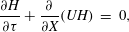
 $$\begin{eqnarray}X\equiv \frac{x}{L},\quad U\equiv \frac{u}{\sqrt{g^{\prime }h_{0}}},\quad H\equiv \frac{h}{h_{0}},\quad \unicode[STIX]{x1D70F}\equiv t\frac{\sqrt{g^{\prime }h_{0}}}{L},\end{eqnarray}$$
where
 $\sqrt{g^{\prime }h_{0}}$
is the typical speed of shallow gravity waves. Now, we can rewrite equations (4.1) in terms of the dimensionless variables as:
 $$\begin{eqnarray}\displaystyle \frac{\unicode[STIX]{x2202}H}{\unicode[STIX]{x2202}\unicode[STIX]{x1D70F}}+\frac{\unicode[STIX]{x2202}}{\unicode[STIX]{x2202}X}(UH) & = & \displaystyle 0,\end{eqnarray}$$
 $$\begin{eqnarray}\displaystyle \frac{\unicode[STIX]{x2202}U}{\unicode[STIX]{x2202}\unicode[STIX]{x1D70F}}+U\frac{\unicode[STIX]{x2202}U}{\unicode[STIX]{x2202}X}+\frac{\unicode[STIX]{x2202}H}{\unicode[STIX]{x2202}X} & = & \displaystyle 0,\end{eqnarray}$$
 $$\begin{eqnarray}\displaystyle U(X,0) & = & \displaystyle 0,\end{eqnarray}$$
 $$\begin{eqnarray}\displaystyle H(X,0) & = & \displaystyle 1.\end{eqnarray}$$
 $C_{\pm }=U\pm \sqrt{H}$
, play a significant role in the initial motion of the flow. Figure 4(a) indicates that the early period occurs when
 $\unicode[STIX]{x1D70F}\lesssim 2$
since it takes
 $t\simeq L/\sqrt{g^{\prime }h_{0}}$
for a gravity wave to travel to the end wall and about the same amount of time to return to the free end. The rarefaction wave is associated with the left-travelling characteristic direction
 $C_{-}\approx -\sqrt{H}$
(since at early times
 $U\approx 0$
). As time evolves,
 $U$
increases and
 $H$
decreases at the edge such that the characteristic direction
 $C_{-}\approx 0$
prevails (choked condition, see e.g. Ungarish (Reference Ungarish2009)), which yields the
 $Fr\approx 1$
condition, where
 $Fr=U/\sqrt{H}|_{(1,\unicode[STIX]{x1D70F})}$
is the Froude number at the edge of the domain. Figure 4(a) also suggests that during the early-time transition period, the
 $Fr$
at the edge increases linearly as
 $Fr=\unicode[STIX]{x1D70F}/\unicode[STIX]{x1D70F}_{t}$
in all the numerical cases, in which
 $\unicode[STIX]{x1D70F}_{t}$
represents the transition time between the early and late time periods. We observed that the transition time
 $\unicode[STIX]{x1D70F}_{t}\approx 2$
for the DNS examples we considered (table 2), except for case D2, when the initial aspect ratio is different from the rest, which influences the transition time. The direct numerical simulations shown in figure 4 also confirm that
 $Fr\simeq 1$
captures the DNS results well after an initial transition period. Hence, based on the analysis of the characteristic directions that is confirmed by the DNS results, the boundary conditions of the two coupled, first-order partial differential equations (PDEs) can be written as:
 $$\begin{eqnarray}U(0,\unicode[STIX]{x1D70F})=0,\text{ and }\left\{\begin{array}{@{}l@{}}\text{Early period }\unicode[STIX]{x1D70F}<\unicode[STIX]{x1D70F}_{t}:Fr=\unicode[STIX]{x1D70F}/\unicode[STIX]{x1D70F}_{t},\\ \text{Late period }\unicode[STIX]{x1D70F}>\unicode[STIX]{x1D70F}_{t}:Fr=1.\end{array}\right.\end{eqnarray}$$
Hence, we have divided our problem into two regimes: (i) an early period where the initial conditions of the flow are important and (ii) a late period, which holds when the effects of initial conditions are no longer important and the solutions describe an asymptotic state of the inertial dynamics. A solution of (4.3) subject to (4.4) and (4.5) describes the dynamics of the flow in both of these regimes and can be obtained numerically. In addition, an analytical solution for the late period is obtainable as we show later. At sufficiently long times, the film becomes so thin that viscous effects become significant; however, we do not aim to investigate this limit here since the flow regime will change into a low Reynolds number flow for which the shallow-water equations (4.1) do not hold anymore (e.g. Zheng et al. (Reference Zheng, Soh, Huppert and Stone2013) studied this viscous limit for gravity current drainage from the edge of a porous reservoir). The limit in which the shallow-water equations are still valid and an inertial phase exists can be established quantitatively. These equations are valid when the time to propagate a gravity wave a distance
 $L$
,
 $L/\sqrt{g^{\prime }h}$
, is shorter than the time at which viscous effects are felt across the film,
 $h^{2}/\unicode[STIX]{x1D708}$
. This means that
 $h/L>Fr/Re$
. Therefore, the focus of the paper is to investigate the late inertial period of this drainage problem, i.e.
 $\unicode[STIX]{x1D70F}\gtrsim \unicode[STIX]{x1D70F}_{t}$
.
The boundary condition for the height during the late period, equation (4.5), is given through this
 $Fr$
relation at the edge, which was found for all times and both regimes using our DNS data as a priori analysis in § 3.2. The
 $Fr$
condition has been a widely used approach to characterize high Reynolds number gravity currents in different contexts. For instance, many such studies impose a constant
 $Fr$
jump condition at the nose of the propagating currents (see Rottman & Simpson Reference Rottman and Simpson1983; Monaghan et al.
Reference Monaghan, Meriaux, Huppert and Monaghan2009; Ungarish Reference Ungarish2009). The
 $Fr$
condition has also been used in other contexts such as in the hydraulic control problems for the flows over obstacles see e.g. Armi & Farmer (Reference Armi and Farmer1986), for maximal flow exchange through a contraction. The control separates a subcritical (
 $Fr<1$
) regime from a supercritical (
 $Fr>1$
) regime. In such configurations, the flow can always travel toward the control (analogous to the gate here) from the subcritical side (similar to our problem) but not from the supercritical side.
4.2 Numerical solutions of the governing PDEs
We numerically solved the shallow-water PDEs (4.3) with given initial conditions (4.4) and boundary conditions (4.5). To do so, we used a finite-volume discretization method and wrote the PDEs in a conservative form. The details of solving the PDEs and the numerical methods employed, along with the validation of the code, are provided in appendix B.
We present solutions for the time evolution of
 $H(X,\unicode[STIX]{x1D70F})$
and
 $U(X,\unicode[STIX]{x1D70F})$
. Figures 5(a) and 5(d), exhibit the height and velocity profiles respectively at early times where the gate is lifted and one can observe the left-travelling wave caused by this release. Once this wave approaches the end wall, it is reflected to the right and hence in figure 5(b,e) we observe a right-travelling wave. Finally, at late times around
 $\unicode[STIX]{x1D70F}\approx 5$
, the profiles shown in figure 5(c,f) reach the similar shapes, which we call the self-similar phase.
Moreover, this flow behaviour is observed in our DNS results. For example, figure 6 shows the profile shape and velocity magnitude contours in the early period, figure 6(a), and the late period, figure 6(b). The velocity magnitude increases in
 $X$
and peaks at the edge. The direction of the velocity vectors in the figure indicates that the flow velocity is more horizontal at late times (figure 6
a) compared to early times (figure 6
b). Hence, this figure confirms the assumption that the flow is mainly horizontal for the shallow-water PDE and it holds when
 $h\ll L$
. The numerical solution of the governing PDEs and the DNS results clearly demonstrate the existence of a self-similar phase. In the next subsection, we will derive the analytical solution for this phase and validate it with the shallow-water solutions. Finally, § 5 will validate the self-similar solutions with the help of experiments and DNS.
Numerical solution of the one-dimensional equations (4.3) in which (a,d) indicate an initial left-travelling wave caused by lifting the gate, (b,e) show the wave reflected by the wall and (c,f) exhibit the late-time profiles that reach a self-similar shape.

The contour of the velocity magnitude (where
 $U$
and
 $V$
respectively represent the horizontal and vertical velocities) for the DNS case D1. (a) The early-time behaviour and (b) the late-time behaviour in the self-similar phase. The black curves show the height of the flow and the arrows indicate the velocity vectors.

4.3 Self-similar solutions
Using equations (4.3), and recognizing that the domain has a fixed length, one can employ an appropriate scaling argument to infer the time evolution of the normalized height and speed of the gravity current in the self-similar phase. For instance, balancing the two terms in the continuity equation (4.3a
) yields
 $H/\unicode[STIX]{x1D70F}\approx -UH$
, which implies
 $U(X,\unicode[STIX]{x1D70F})\propto \unicode[STIX]{x1D70F}^{-1}$
. A quantitative comparison will be made below. Using this time dependence of the scaled velocity and balancing the three terms in (4.3b
) leads to
 $H(X,\unicode[STIX]{x1D70F})\propto \unicode[STIX]{x1D70F}^{-2}$
. Thus, we introduce
 $$\begin{eqnarray}\displaystyle & \displaystyle U(X,\unicode[STIX]{x1D70F})=(\unicode[STIX]{x1D70F}+\unicode[STIX]{x1D6FE})^{-1}\widetilde{U}(X), & \displaystyle\end{eqnarray}$$
 $$\begin{eqnarray}\displaystyle & \displaystyle H(X,\unicode[STIX]{x1D70F})=(\unicode[STIX]{x1D70F}+\unicode[STIX]{x1D6FE})^{-2}\widetilde{H}(X), & \displaystyle\end{eqnarray}$$
 $\widetilde{U}$
and
 $\widetilde{H}$
are, respectively, the similarity functions for velocity and height, and
 $\unicode[STIX]{x1D6FE}$
is a constant time shift that will be determined to match the shallow-water PDE solutions (e.g. the fluid volume or the fluid height at the edge). Substituting equations (4.6) into (4.3) yields two nonlinearly coupled first-order ordinary differential equations (ODEs)
 $$\begin{eqnarray}\displaystyle & \displaystyle -2\widetilde{H}+\frac{\text{d}}{\text{d}X}(\widetilde{U}\widetilde{H})=0, & \displaystyle\end{eqnarray}$$
 $$\begin{eqnarray}\displaystyle & \displaystyle -\widetilde{U}+\widetilde{U}\frac{\text{d}\widetilde{U}}{\text{d}X}+\frac{\text{d}\widetilde{H}}{\text{d}X}=0, & \displaystyle\end{eqnarray}$$
 $$\begin{eqnarray}\left.\widetilde{U}(0)=0,\quad \frac{\widetilde{U}}{\sqrt{\widetilde{H}}}\right|_{X=1}=Fr.\end{eqnarray}$$
We will integrate our derived ODE system in equations (4.7) analytically. The two ODEs can be rearranged as
 $$\begin{eqnarray}\displaystyle & \displaystyle \frac{\text{d}\widetilde{U}}{\text{d}\widetilde{X}}=\frac{2\widetilde{H}-\widetilde{U}^{2}}{\widetilde{H}-\widetilde{U}^{2}}, & \displaystyle\end{eqnarray}$$
 $$\begin{eqnarray}\displaystyle & \displaystyle \frac{\text{d}\widetilde{H}}{\text{d}\widetilde{X}}=-\frac{\widetilde{U}\widetilde{H}}{\widetilde{H}-\widetilde{U}^{2}}. & \displaystyle\end{eqnarray}$$
 $\widetilde{U}(\widetilde{H})$
,
 $$\begin{eqnarray}\frac{\text{d}\widetilde{U}}{\text{d}\widetilde{H}}=\frac{\widetilde{U}^{2}-2\widetilde{H}}{\widetilde{U}\widetilde{H}}.\end{eqnarray}$$
Integrating this equation and using the left boundary condition
 $\widetilde{U}(X=0)=0$
with
 $\widetilde{H}(0)$
(to be determined) gives
 $$\begin{eqnarray}\widetilde{U}(\widetilde{H})=2\widetilde{H}^{1/2}(1-\widetilde{H}/\widetilde{H}(0))^{1/2}.\end{eqnarray}$$
It then follows that the
 $Fr$
condition at the free end,
 $\widetilde{U}/\sqrt{\widetilde{H}}\rightarrow 1$
as
 $X\rightarrow 1$
, leads to
 $\widetilde{H}(1)/\widetilde{H}(0)=3/4$
. We can then construct the shape of the current by substituting into equation (4.9b
) to find
 $$\begin{eqnarray}\frac{\text{d}\widetilde{H}}{\text{d}X}=\frac{2}{3}\frac{\widetilde{H}^{1/2}(1-\widetilde{H}/\widetilde{H}(0))^{1/2}}{\displaystyle \left(1-\frac{4\widetilde{H}}{3\widetilde{H}(0)}\right)}.\end{eqnarray}$$
Integrating this equation we obtain an analytical solution for the profile shape as
 $$\begin{eqnarray}X=-\frac{\unicode[STIX]{x03C0}}{2}\sqrt{\widetilde{H}(0)}+2\sqrt{\widetilde{H}(1-\widetilde{H}/\widetilde{H}(0))}+\sqrt{\widetilde{H}(0)}\arctan \left(\sqrt{\widetilde{H}/(\widetilde{H}(0)-\widetilde{H})}\right).\end{eqnarray}$$
Evaluating (4.13) at
 $X=1$
and considering
 $\widetilde{H}(1)/\widetilde{H}(0)=3/4$
we find
 $\widetilde{H}(0)=[6/(3\sqrt{3}-\unicode[STIX]{x03C0})]^{2}\approx 8.5$
. The corresponding velocity distribution
 $U(X)$
follows from (4.11).
Based on the obtained analytical solutions, the constant time shift,
 $\unicode[STIX]{x1D6FE}$
, in (4.6b
) can be determined by matching the fluid height at the edge. Following our numerical solutions of the governing PDEs in figure 5
 $H(X=1,\unicode[STIX]{x1D70F})$
can be found, and considering
 $\widetilde{H}(1)\approx 8.5\times 3/4$
we obtain
 $\unicode[STIX]{x1D6FE}\approx 2$
. The validity of these solutions compared to the DNS and experimental results will be assessed in the next section.
We note that many of the previous similarity solutions are for problems in which the volume of the gravity current does not change, e.g. the classic paper by Rottman & Simpson (Reference Rottman and Simpson1983). The dam-break problems have constant volume; however, the volume in our domain decreases and thus we have different scaling results for the time dependence and a different boundary condition, i.e.
 $Fr\simeq 1$
at the edge. Hence, our self-similar solutions are different from the self-similar flows in the reservoir domain of spreading gravity current problem, produced from a sudden dam-break mechanism (e.g. Ungarish Reference Ungarish2009, ch. 10). In particular, our approach in this paper was to first balance the terms in the continuity and momentum equations, considering the fixed length of the domain, to infer the time dependence in the similarity phase (4.6) and then use them to obtain the self-similar profile shapes.
We have also plotted the PDE solutions of equations (4.3) against the solutions of the ODEs in equations (4.7) at different times to investigate whether the PDE solutions will converge to the obtained self-similar solutions. As figure 7 shows, the PDE solutions first undergo an early adjustment phase and finally they approach the self-similar solution after some small oscillations. These results clearly demonstrate good agreement between the self-similar solution and the governing PDE solutions for both the velocity and height profiles.
Time evolution of (a) the profile shape
 $H(X,\unicode[STIX]{x1D70F})$
and (b) the velocity field
 $U(X,\unicode[STIX]{x1D70F})$
(dashed lines) from numerically solving the one-dimensional PDE (4.3) subject to (4.4) and (4.5). The self-similar solutions are also plotted (solid lines) from (4.13).

5 Validation of the reduced-order ODE model
In this section, we examine the flow behaviour and validate the reduced-order ODE model from § 4 using the experimental and DNS results, as presented in §§ 2 and 3 respectively.
5.1 Validating the scaling arguments and self-similar solutions using experiments
In order to validate the scaling arguments in § 4, we have plotted in figure 8(a) the height time series for all experimental measurements recorded in the middle of the domain (
 $x=L/2$
). Figure 8(b) depicts the same data with dimensionless variables, in which all six curves collapse very well at late times. For comparison, the solid line indicates the
 $\unicode[STIX]{x1D70F}^{-2}$
scaling that our reduced-order model (4.6b
) predicts. We can observe from figure 8(b) that the height at
 $X=1/2$
decreases as
 $(\unicode[STIX]{x1D70F}+2)^{-2}$
in the similarity phase,
 $\unicode[STIX]{x1D70F}\gtrsim 2$
, and our scaling theory shows good agreement with the experimental results.
Time evolution of the height of the gravity current at the centre of the tank (
 $X=0.5$
) for all of the experiments (E1–E6): (a) dimensional data and (b) rescaled data. The theoretical prediction of the self-similar solution, i.e.
 $(\unicode[STIX]{x1D70F}+2)^{-2}\widetilde{H}(0.5)$
, is also plotted in (b), which agrees well with the rescaled heights after an initial transition period,
 $\unicode[STIX]{x1D70F}\approx 2$
.

Now we compare the experimental data for the profile shape of the current with the results of the reduced-order model. Figure 9(a) displays the dimensional values of the profile evolution while figure 9(b) shows the non-dimensional values. This figure exhibits good agreement between the experiments in the self-similar phase and the reduced-order model; the maximum relative error is less than 10 % for each measured point of case E6 that is shown. The transition period is also clear from these results where the normalized height of the flow gradually increases up to the similarity phase.
Next, we present the experimental depth profiles at late times (
 $\unicode[STIX]{x1D70F}\approx 5$
) when all data should be in the similarity phase. The results in figure 10 collapse well after non-dimensionalizing for all of the performed experiments. Note that in the self-similar phase,
 $Re=uh/\unicode[STIX]{x1D708}_{c}=Fr\sqrt{g^{\prime }h}h/\unicode[STIX]{x1D708}_{c}$
, which is approximately
 $10^{2}{-}10^{4}$
at
 $\unicode[STIX]{x1D70F}\approx 5$
for the different cases. This good agreement demonstrates that our reduced-order model is able to accurately predict the gravity current behaviour in the self-similar phase for different conditions.

The profile shapes of all the experiments in the self-similar phase: (a) dimensional data and (b) rescaled data. The prediction of the self-similar solution is plotted in (b), which is found to agree well with the rescaled experimental results after the transition period.

5.2 Validating scaling arguments and self-similar solutions using DNS
The scaling arguments implied that the heights of the profiles have to decrease as
 $\unicode[STIX]{x1D70F}^{-2}$
in the self-similar phase. Figure 11 shows the results of the DNS at
 $X=0$
,
 $X=1$
and an averaged height throughout the domain for case D1. The results in the figure demonstrate that the DNS data also confirm our scaling arguments.
Height versus time for the case D1 of the DNS results: (a) dimensional data and (b) rescaled data. The slope of the scaling argument of equation (4.6b ) is shown in (b), matching the DNS data well.

To further validate our scaling arguments, the height time series at
 $X=1/2$
for all the DNS results are investigated. Figure 12 shows the depth time series for all cases in terms of raw data (figure 12
a) and non-dimensionalized values (figure 12
b). All the simulations collapse well after non-dimensionalization and match with the theoretical solution obtained from (4.6).
Height versus time for the DNS data at
 $X=1/2$
for all cases: (a) dimensional data and (b) rescaled data. The prediction of the self-similar solution, i.e.
 $(\unicode[STIX]{x1D70F}+2)^{-2}\widetilde{H}(0.5)$
, is plotted in (b), which agrees with the rescaled heights after the transition period.

Furthermore, non-dimensional depth profiles from DNS data are in good agreement with the obtained analytical similarity solution. Figure 13 depicts our dimensional DNS results and their non-dimensional values versus the similarity solution.
The profile shapes of the DNS results in the self-similar phase: (a) dimensional data and (b) rescaled data. The prediction of the similarity solution is shown in (b). The oscillations for case D2 are related to the vertical resolution and numerical accuracy of the simulations.

6 Discussion and implications
6.1 Practical applications
One of the practical applications of this reduced-order model could be in characterizing reservoir drainage problems in any configuration that results in
 $Fr\approx 1$
at the boundary (free fall with a perpendicular edge as in our experiments and DNS or simply a very steep slope on the ambient fluid side of the problem). For instance, when a wall in a fluid container is removed, when a tank of fluid (e.g. a tank of water in various structures) breaks or when a spillway is damaged, the discharge rate in the similarity phase could be predicted by our reduced-order model. A potential practical application concerns a break of a spillway structure on top of a dam such as the one that recently occurred in the Oroville dam in California (http://www.cnn.
com/2017/02/12/us/california-oroville-dam-failure/). Figure 14(a) displays the DNS results for the volume
 $V_{out}$
that is spilled from the domain. For the initial conditions we considered, the results indicate that
 ${\approx}50\,\%$
of the initial volume exits at early times (initial adjustment period
 $\unicode[STIX]{x1D70F}\lesssim 2$
) and
 ${\approx}40\,\%$
of the initial volume is removed during the similarity phase by the end of the simulations (which takes approximately two times longer than the initial adjustment period). The discharge rate of this drainage is also shown in figure 14(b). The discharge gradually increases at early time periods and, after reaching a maximum, it decreases in the similarity phase. Note that at early periods, the drainage rates might be approximated by some available gravity current solutions using simplified assumptions although further research is required to establish the interface shape of the draining edge and its dynamics in the initial adjustment period. For instance, the DNS drainage value is in good agreement with the simple dam-break solutions (i.e.
 $Q(X=1,\unicode[STIX]{x1D70F}=2)=8/27$
see Ungarish (Reference Ungarish2009)) for 1
 ${\lesssim}\unicode[STIX]{x1D70F}\lesssim 2$
. However, significant discrepancies with our problem are seen for
 $\unicode[STIX]{x1D70F}\lesssim 1$
and also for the predicted profile shapes of dam-break solutions (not shown), which are due to the different physics of the two problems. Alternatively, the drainage values can be obtained from the numerical solutions of the PDEs in § 4.2. The numerical solutions of the shallow-water equations in figure 14 display a good agreement with DNS results. Furthermore, figure 14 shows that our reduced-order model is in a good agreement with the DNS results during the similarity period and hence it could be used in this context for predicting the discharge rates in practical applications or engineering designs.
In fact, the geometry of the problem we have considered (figures 1(c) and 2) is a common shape for open channel flows. Therefore, the analysis presented here could also be useful for hydraulic engineering and design where edge flows occur. Furthermore, the analysis could help to understand the flow behaviour after a dam break where the released fluid falls from the broken structure or for describing the behaviour of an overflow caused by the excess inflow due to rain or other reasons. This analysis could also be extended to other cross-sectional shapes such as V-shaped or curved geometries (see e.g. Ungarish Reference Ungarish2013b ; Zemach & Ungarish Reference Zemach and Ungarish2013, for non-rectangular cross-section studies of gravity currents) and for ventilation problems where the interface shape and the discharge rates of cold (dense) air and hot (light) air systems in a building are sought.
An example of reservoir drainage as one of the applications of drainage from an edge. When a wall in a tank of a fluid is removed or when a reservoir such as an aquarium breaks, the dynamics of the interface shape, the discharge and the volume removal rate could be described using our results. The ratio of the removed volume,
 $V_{out}$
, over the initial volume,
 $V_{0}$
, for three cases of our DNS results are shown in (a). The prediction of the self-similar solutions for the discharge, i.e.
 $\widetilde{Q}(1)=(\unicode[STIX]{x1D70F}+2)^{-3}\widetilde{H}(1)^{3/2}$
, is plotted in (b), which agrees with the rescaled discharge in the similarity phase. An approximate dam-break solution for the initial slumping phase is also plotted; it works well for
 $1\lesssim \unicode[STIX]{x1D70F}\lesssim 2$
. The numerical shallow-water PDE solutions obtained in § 4.2, which are plotted in (b), agree well with the DNS results.

6.2 Model assumptions and limitations
In our analysis, we have employed the shallow-water equations, which are derived from the Euler equations. It is assumed that the motion in the ambient fluid has negligible effects on the flow of the dense fluid. Furthermore, the shallow-water equations are vertically averaged and hence two-dimensional effects are neglected, which could be important especially during the early-time period when the heights could be comparable with the length but not during the similarity phase that we focused on here. At sufficiently long times, viscous effects become important and eventually dominate the inertial effects; however, we do not consider such long-time behaviour. We also ignored entrainment and surface tension effects, which are typically small in the kinds of problems studied here.
7 Summary
In this study, we investigated drainage of fluid from the edge of a reservoir. We found two distinct high Reynolds number regimes for this problem: (i) an early adjustment period and (ii) a late-time similarity phase where the depth profiles have self-similar shapes.
Using scaling arguments, we suggested that the height of the flow varies as
 $\unicode[STIX]{x1D70F}^{-2}$
in the self-similar phase, where
 $\unicode[STIX]{x1D70F}$
is time non-dimensionalized by the ratio of the length of the domain and the typical gravity wave speed. The scaling results were validated against laboratory experiments and direct numerical simulations of the full two-dimensional problem.
Based on the scaling arguments, we defined appropriate similarity variables, and the shallow-water equations led to two nonlinearly coupled ODEs. We then analytically solved the coupled ODEs by imposing a zero velocity boundary condition at the left end wall, and imposed a constant Froude number condition at the right edge of the domain where the DNS results confirmed there is a chocked condition with
 $Fr\simeq 1$
. The validity of the second assumption was investigated and confirmed through DNS data. Good agreement was found between the experiments, DNS and the reduced-order model. The reduced-order model for the edge drainage of an inertial gravity current could be useful for many applications as indicated in § 6.1. For the typical rectangular initial conditions we considered here, the simulation results indicate that
 ${\approx}50\,\%$
of the initial volume exits the reservoir at early times (
 $\unicode[STIX]{x1D70F}\lesssim 2$
) and
 ${\approx}40\,\%$
of the initial volume is removed during the similarity phase (inertia-dominated regime), when the new similarity solution we identified from the reduced-order model applies.
Acknowledgements
We thank the helpful and insightful feedback of the referees that improved our paper. This work started with M.M. doing a project at Princeton University in a graduate course offered by Z.Z. and H.A.S. Z.Z. acknowledges partial support from the Princeton CMI Young Investigator Award. The direct numerical simulations were performed on the Della computer clusters of Princeton University.
Supplementary material
Supplementary material is available at https://doi.org/10.1017/jfm.2017.480.
Appendix A. Details of the direct numerical solutions
We use the interFoam multiphase solver of OpenFoam v2.4 to conduct the direct numerical simulations (see http://www.openfoam.org/version2.4.0/ and Deshpande, Anumolu & Trujillo (Reference Deshpande, Anumolu and Trujillo2012a
) for its performance and validation). The code solves the mass conservation equation for the fluid considering two fluid phases in each control volume by introducing the phase fraction
 $\unicode[STIX]{x1D6FC}$
according to
 $$\begin{eqnarray}\left.\begin{array}{@{}l@{}}\unicode[STIX]{x1D6FC}=1\quad \text{liquid,}\\ 0<\unicode[STIX]{x1D6FC}<1\quad \text{interface,}\\ \unicode[STIX]{x1D6FC}=0\quad \text{gas.}\end{array}\right\}\end{eqnarray}$$
Hence, the mass conservation equation is written as:
 $$\begin{eqnarray}\frac{\unicode[STIX]{x2202}\unicode[STIX]{x1D70C}}{\unicode[STIX]{x2202}t}+\unicode[STIX]{x1D735}\boldsymbol{\cdot }(\unicode[STIX]{x1D70C}\boldsymbol{u})=0,\end{eqnarray}$$
where the phase fraction above can be used to describe the density field as:
 $$\begin{eqnarray}\unicode[STIX]{x1D70C}=\unicode[STIX]{x1D6FC}\unicode[STIX]{x1D70C}_{c}+(1-\unicode[STIX]{x1D6FC})\unicode[STIX]{x1D70C}_{a}.\end{eqnarray}$$
The governing momentum equation of this solver is:
 $$\begin{eqnarray}\frac{\unicode[STIX]{x2202}\boldsymbol{u}}{\unicode[STIX]{x2202}t}+\boldsymbol{u}\boldsymbol{\cdot }\unicode[STIX]{x1D735}\boldsymbol{u}=-\frac{1}{\unicode[STIX]{x1D70C}}\unicode[STIX]{x1D735}p+\unicode[STIX]{x1D708}\unicode[STIX]{x1D6FB}^{2}\boldsymbol{u}+\boldsymbol{F}_{\unicode[STIX]{x1D70E}}+\boldsymbol{g},\end{eqnarray}$$
where
 $\unicode[STIX]{x1D708}=\unicode[STIX]{x1D6FC}\unicode[STIX]{x1D708}_{c}+(1-\unicode[STIX]{x1D6FC})\unicode[STIX]{x1D708}_{a}$
. In (A 4),
 $\boldsymbol{F}_{\unicode[STIX]{x1D70E}}=2\unicode[STIX]{x1D70E}\unicode[STIX]{x1D705}(\unicode[STIX]{x1D70C}/\unicode[STIX]{x1D70C}_{a}+\unicode[STIX]{x1D70C}_{c})\unicode[STIX]{x1D735}\unicode[STIX]{x1D6FC}$
denotes the surface tension force,
 $\unicode[STIX]{x1D705}$
represents the interface curvature and
 $\unicode[STIX]{x1D70E}$
is the surface tension coefficient. Here
 $\unicode[STIX]{x1D70C}_{a}$
and
 $\unicode[STIX]{x1D708}_{a}$
denote, respectively, the density and kinematic viscosity of the ambient fluid and
 $\unicode[STIX]{x1D70C}_{c}$
and
 $\unicode[STIX]{x1D708}_{c}$
denote, respectively, the density and kinematic viscosity of the gravity current. Note that a Poisson equation for the pressure is substituted for the mass conservation equation using the pressure implicit with splitting of operators algorithm (Issa Reference Issa1986). For all the simulations, we set
 $\unicode[STIX]{x1D70E}=0.07~\text{N}~\text{m}^{-1}$
,
 $\unicode[STIX]{x1D708}_{c}=10^{-6}~\text{m}^{2}~\text{s}^{-1}$
, and
 $\unicode[STIX]{x1D708}_{a}=1.5\times 10^{-5}~\text{m}^{2}~\text{s}^{-1}$
. Although our simulations involve surface tension forces, they do not play an important role in the dynamics of our flow during the initial phases we focus on since the Weber number,
 $\unicode[STIX]{x1D70C}u^{2}h/\unicode[STIX]{x1D70E}\approx 10-10^{5}$
, is large. The capillary number,
 $\unicode[STIX]{x1D707}u/\unicode[STIX]{x1D70E}$
which varies in time, is of the order of
 ${\approx}0.01$
here. A DNS test we conducted without the surface tension force showed less than 2 % difference in the profile height of the gravity current during the simulation period, which confirms the insignificant impact of this force on the dynamics of our flow. The Bond number is
 $Bo=\unicode[STIX]{x1D70C}gL^{2}/\unicode[STIX]{x1D70E}\approx 6000$
; hence, the effects of surface tension must be small for this gravity-driven motion. We included this force in the simulations in order to better represent a realistic scenario at small scales and to avoid numerical instabilities at the small length scales of the interface.
Numerical domain of the direct numerical simulations for case D1, which includes five subdomains with different resolutions. The numbers in (b) (not to scale) indicate the number of grids in the simulation D1.

As an example of the simulations we performed, figure 15 shows the computational domains and the number of control volumes for case D1. We set the liquid in subdomain (d) of figure 15 (blue region) with higher resolution according to the geometry indicated in table 2 and then ran the simulations. The initial condition of our simulations for the phase fraction
 $\unicode[STIX]{x1D6FC}$
is shown in 15(a) and the initial condition for the velocity is zero everywhere, which can be respectively written as
 $$\begin{eqnarray}\displaystyle & \displaystyle \left.\begin{array}{@{}l@{}}\unicode[STIX]{x1D6FC}=1\quad 0<x<L\text{ and }1<h\leqslant 1+h_{0}\\ \unicode[STIX]{x1D6FC}=0\quad \text{everywhere else in the domain,}\end{array}\right\} & \displaystyle\end{eqnarray}$$
 $$\begin{eqnarray}\displaystyle & \displaystyle \boldsymbol{u}(t=0)=\mathbf{0}. & \displaystyle\end{eqnarray}$$
The boundaries shown in figure 15(a) are no-slip impermeable walls. Thus, the boundary conditions at all wall boundaries for the velocity field can be written as
 $$\begin{eqnarray}\boldsymbol{u}=\mathbf{0}\quad \text{for wall boundaries.}\end{eqnarray}$$
To satisfy the impermeable wall boundary condition, the pressure Poisson equation must have a vanishing wall-normal pressure gradient at the wall
 $\unicode[STIX]{x2202}p/\unicode[STIX]{x2202}n=0$
, where
 $n$
is
 $x$
for vertical walls and
 $z$
for horizontal walls. In the code, this is done by extrapolating the pressure field from the fluid side of the interface to satisfy this vanishing pressure gradient requirement at the wall (see Rhie & Chow Reference Rhie and Chow1983). Moreover, the boundary condition for
 $\unicode[STIX]{x1D6FC}$
is also zero gradient at the wall boundaries. Note that the only important wall boundaries for our problem are the left wall and the wall below the fluid since the inertial phase is over before the flow reaches the bottom or the right wall. For time advancement, an implicit Euler method is used. The spatial discretization is based on the standard finite-volume discretization, which uses the interpolation from cell centres to face centres by central differencing. The divergence schemes are based on Gaussian integration with a second-order interpolation. Note that we added an initial noise to account for possible turbulent effects of the gravity current and ran case D1 again, but the instabilities did not grow in time particularly in the late-time self-similar phase since
 $Re\approx 10^{2}{-}10^{4}$
; hence we did not add noise to the DNS cases reported in the paper. The flow therefore does not appear to transition to turbulence. Nevertheless, we set the spatial resolution such that
 $\unicode[STIX]{x0394}x/h_{0}(=2-5\times 10^{-3})\approx 2\unicode[STIX]{x1D702}/L=2/Re^{3/4}\approx 2-6\times 10^{-3}$
in our simulations, where
 $\unicode[STIX]{x1D702}$
is the Kolmogorov length scale. Note that in numerical simulations of geophysical flows with significant
 $Re\gtrsim 10^{4}$
, turbulence effects must be considered, e.g. in geophysical boundary layers (Momen & Bou-Zeid Reference Momen and Bou-Zeid2017), or in rough surfaces of rivers and oceans (Tokyay, Constantinescu & Meiburg Reference Tokyay, Constantinescu and Meiburg2011). Shear instabilities can develop along the interface when the mixing occurs and the Richardson number,
 $g|\unicode[STIX]{x1D735}\unicode[STIX]{x1D70C}|/\unicode[STIX]{x1D70C}|\unicode[STIX]{x1D735}u|^{2}$
which shows the relative strength of the stratification over the vertical shear, is sufficiently low. In our DNS cases, the density difference between the current and the ambient fluid is large (see table 2) and the Richardson number is high and hence this instability is not observed. We also doubled the resolution of case D1 for the convergence test and did not observe any significant differences between the simulations.
The interFoam solver was previously tested on inertia-dominated flows and was found to perform very well in such conditions even with modest grid resolutions (see Deshpande et al. Reference Deshpande, Anumolu and Trujillo2012a ). The interFoam solver of OpenFoam has also been previously used and/or validated against experiments in many other studies (see, e.g. Berberovic et al. Reference Berberovic, van Hinsberg, Jakirlic, Roisman and Tropea2008; Liu & Garcia Reference Liu and Garcia2008; Deshpande et al. Reference Deshpande, Trujillo, Wu and Chahine2012b ; Moukalled, Mangani & Darwish Reference Moukalled, Mangani and Darwish2015).
These simulations were conducted with MPI parallel format on 16 nodes of the Princeton Della computer clusters. The total number of control volumes was approximately
 $10^{6}$
–
 $10^{7}$
depending on the resolution and size of each performed simulation.
Appendix B. Numerical details of the PDE code and its validation
We used a finite-volume method to solve equation (4.3). We write the momentum equation in the conservative form as:
 $$\begin{eqnarray}\left.\begin{array}{@{}l@{}}\displaystyle \frac{\unicode[STIX]{x2202}H}{\unicode[STIX]{x2202}\unicode[STIX]{x1D70F}}+\frac{\unicode[STIX]{x2202}}{\unicode[STIX]{x2202}X}(HU)=0,\\ \displaystyle \frac{\unicode[STIX]{x2202}(HU)}{\unicode[STIX]{x2202}\unicode[STIX]{x1D70F}}+\frac{\unicode[STIX]{x2202}(H^{2}/2+HU^{2})}{\unicode[STIX]{x2202}X}=0.\end{array}\right\}\end{eqnarray}$$
Now we define the variables:
 $$\begin{eqnarray}\boldsymbol{S}=\left(\begin{array}{@{}c@{}}H\\ HU\end{array}\right),\quad \boldsymbol{F}=\left(\begin{array}{@{}c@{}}HU\\ H^{2}/2\end{array}\right),\quad \boldsymbol{G}=\left(\begin{array}{@{}c@{}}0\\ HU^{2}\end{array}\right).\end{eqnarray}$$
Next, we rewrite equations (B 1) as
 $$\begin{eqnarray}\frac{\unicode[STIX]{x2202}\boldsymbol{S}}{\unicode[STIX]{x2202}\unicode[STIX]{x1D70F}}+\frac{\unicode[STIX]{x2202}(\boldsymbol{F}+\boldsymbol{G})}{\unicode[STIX]{x2202}X}=\mathbf{0},\end{eqnarray}$$
which gives a one-dimensional hyperbolic conservation law. Then, we discretize this equation using an upwind scheme for the advective term, a centred scheme for other spatial derivatives and a third-order Adams–Bashforth scheme in time as
 $$\begin{eqnarray}\displaystyle & & \displaystyle \frac{\boldsymbol{S}_{i}^{j+1}-\boldsymbol{S}_{i}^{j}}{\unicode[STIX]{x0394}\unicode[STIX]{x1D70F}}+\frac{23}{12}\left(\frac{\boldsymbol{F}_{i+1}^{j}-\boldsymbol{F}_{i-1}^{j}}{2\unicode[STIX]{x0394}X}+\frac{\boldsymbol{G}_{i}^{j}-\boldsymbol{G}_{i-1}^{j}}{\unicode[STIX]{x0394}X}\right)-\frac{4}{3}\left(\frac{\boldsymbol{F}_{i+1}^{j-1}-\boldsymbol{F}_{i-1}^{j-1}}{2\unicode[STIX]{x0394}X}+\frac{\boldsymbol{G}_{i}^{j-1}-\boldsymbol{G}_{i-1}^{j-1}}{\unicode[STIX]{x0394}X}\right)\nonumber\\ \displaystyle & & \displaystyle \quad +\,\frac{5}{12}\left(\frac{\boldsymbol{F}_{i+1}^{j-2}-\boldsymbol{F}_{i-1}^{j-2}}{2\unicode[STIX]{x0394}X}+\frac{\boldsymbol{G}_{i}^{j-2}-\boldsymbol{G}_{i-1}^{j-2}}{\unicode[STIX]{x0394}X}\right)=\mathbf{0}\quad \text{for }U_{i}^{j}>0,\end{eqnarray}$$
 $$\begin{eqnarray}\displaystyle & & \displaystyle \frac{\boldsymbol{S}_{i}^{j+1}-\boldsymbol{S}_{i}^{j}}{\unicode[STIX]{x0394}\unicode[STIX]{x1D70F}}+\frac{23}{12}\left(\frac{\boldsymbol{F}_{i+1}^{j}-\boldsymbol{F}_{i-1}^{j}}{2\unicode[STIX]{x0394}X}+\frac{\boldsymbol{G}_{i+1}^{j}-\boldsymbol{G}_{i}^{j}}{\unicode[STIX]{x0394}X}\right)-\frac{4}{3}\left(\frac{\boldsymbol{F}_{i+1}^{j-1}-\boldsymbol{F}_{i-1}^{j-1}}{2\unicode[STIX]{x0394}X}+\frac{\boldsymbol{G}_{i+1}^{j-1}-\boldsymbol{G}_{i}^{j-1}}{\unicode[STIX]{x0394}X}\right)\nonumber\\ \displaystyle & & \displaystyle \quad +\,\frac{5}{12}\left(\frac{\boldsymbol{F}_{i+1}^{j-2}-\boldsymbol{F}_{i-1}^{j-2}}{2\unicode[STIX]{x0394}X}+\frac{\boldsymbol{G}_{i+1}^{j-2}-\boldsymbol{G}_{i}^{j-2}}{\unicode[STIX]{x0394}X}\right)=\mathbf{0}\quad \text{for }U_{i}^{j}<0.\end{eqnarray}$$
 $$\begin{eqnarray}\boldsymbol{S}_{i}^{0}=\left(\begin{array}{@{}c@{}}H_{0}^{0}\\ 0\end{array}\right),\quad \boldsymbol{S}_{0}^{j}=\left(\begin{array}{@{}c@{}}H_{1}^{j}\\ 0\end{array}\right).\end{eqnarray}$$
For the right boundary, we solve equation (B 4) with an upwind scheme in space and a third-order Adams–Bashforth scheme in time by increasing the
 $Fr$
at the early time period and then applying the Froude number condition at the edge.
We have validated the code for the spreading problem of Rottman & Simpson (Reference Rottman and Simpson1983), corresponding to a finite-volume release of fluid by lifting a lock gate. Figure 16 exhibits a good match between the results of our code and the previous numerical solutions of Rottman & Simpson (Reference Rottman and Simpson1983), which were based on the method of characteristics.
Validation of the PDE code with the numerical solutions of Rottman & Simpson (Reference Rottman and Simpson1983) with
 $Fr=\sqrt{2}$
. The dashed curves show our results and the solid lines are the solutions of Rottman & Simpson (Reference Rottman and Simpson1983). Here
 $x$
is the horizontal coordinate,
 $t$
is time,
 $x_{0}$
is the initial length of the gravity current,
 $h_{0}$
is the initial depth,
 $h_{1}$
is the height of the gravity current and
 $t_{0}\equiv x_{0}/(g^{\prime }h_{0})^{1/2}$
denotes a timescale.



