1. Introduction
Marine navigation, positioning and the development of marine resources are increasingly of concern for most countries around the world. Research on underwater navigation and positioning technology has become increasingly mature (Yang et al., Reference Yang, Liu, Sun, Xu and Zeng2020). The construction of the submarine geodetic reference network is extremely difficult, and the technical requirements for the calibration of reference points are rigorous. Hence, more precise underwater positioning is required. The GNSS-A system uses acoustic technology to achieve underwater positioning, assisted by global navigation satellite system (GNSS) positioning on the sea surface, consequently completing the joint measurement of land and ocean space positions (Fujita et al., Reference Fujita, Ishikawa, Mochizuki, Sato, Toyama, Katayama, Matsumoto, Yabuki and Asada2006). However, due to the particularity of the water environment, underwater positioning has the characteristics of being dynamic and non-repeatable compared with land positioning. Under the current observation conditions, the time measurement error can be controlled to within 0·1 ms (Zhao et al., Reference Zhao, S., Wang, Z. and Liu, H.2018). Thus, the sound speed error is the main factor affecting the positioning accuracy. The traditional calculation of straight-line distance is based on the assumption that the sound speed is a constant in the water. Actually, the sound speed is a complex function of temperature, salinity and pressure, which have strong temporal and spatial characteristics (Liu et al., Reference Liu, Xue, Qu, G., Lu and Qi2020). The change of sound speed with depth is expressed by the sound speed profile (SSP). SSP measurement is generally obtained by direct measurement using the ‘underwater sound speed meter’ (Jamshidi and Abu Bakar, Reference Jamshidi and Abu Bakar2010). Munk proposed the now classic Munk-SSP model, which is suitable for the deep sea, based on the stratification characteristics of the density structure of the measured deep sea (Munk, Reference Munk1974). The acoustic ray bending error is caused by the refraction of sound waves during the propagation process due to the change of sound speed, and the propagation of sound signals obeys Snell's law (Zhao et al., Reference Zhao, J., Li, J. and Li, M.2009). Zhao's research shows that sound speed error is the main source of error in underwater positioning, and cannot be ignored in high-precision positioning (Zhao et al., Reference Zhao, J and Liang, W2019). Therefore, the correction of the sound speed is one of the key technologies to improve the accuracy of underwater acoustic positioning.
The average sound speed positioning model directly uses a single sound speed for distance measurement. This model is simple and efficient, but it ignores the effect of sound speed errors. Based on the Taylor series expansion, a sound speed correction method through numerical simulation has been proposed, which is suitable for different SSP. However, when the elevation angle is small, the sound speed error is larger (Li, Reference Li, S.2015). The empirical sound speed method can quickly calculate the sound speed, but it requires a large amount of experimental research, and the determination of coefficients is complicated (Zhao et al., Reference Zhao, J. and Liu, J2008). Others have proposed to use a neural network method for sound speed correction, but the model and method are not mature enough – follow-up research is still needed. Vincent and Hu (Reference Vincent and Hu2000) put forward the concept of effective sound speed based on ray theory. To meet the real-time performance of the positioning system, a two-dimensional table of water depth and pitch angle is established to achieve rapid acquisition of sound speed. However, the process of establishing the table requires extensive calculation and storage space. Ray tracing technology uses the layer addition method to calculate the acoustic ray propagation path. Based on the accurate measurement of sound speed, it reduces the influence of the acoustic ray bending error to obtain high-precision three-dimensional coordinates of underwater target points (Sakic et al., Reference Sakic, Ballu, Crawford and Woeppelmann2018; Wang et al., Reference Wang, Li, Liang and Fu2009). The processing of residual information is also very important for the analysis of positioning accuracy, and a cubature Kalman filter with a multi-rate residual correction algorithm is proposed to fuse inertial navigation systems (INS) and polarization compass (PC) navigation outputs with different sampling frequencies (Zhao et al., Reference Zhao, Liu, Zhao and Wang2020). The accuracy of the above algorithm is higher than that of the average sound speed positioning model, however, it also has problems, such as complex positioning model and low calculation efficiency (Sun, Reference Sun, W.2007).
Incident angle related errors are an important error source in positioning, including ranging system noise errors, sound speed errors and control point errors. Studies have shown that the impact of sound speed on distance measurement and positioning is related to the beam incident angle and depth, which is significant and cannot be ignored (Zhao et al., Reference Zhao, J and Liang, W2019). Therefore, when the observation configuration is not good, the range of incident angle is large, and the error of the average sound speed model has a significant influence, leading to inaccurate positioning results. The motivation of this research is to improve the efficiency of the solution without losing, or only slightly reducing, the accuracy. This paper introduces the principle of the underwater geometric positioning solution based on the average sound speed, and gives the method of calculation of the average sound speed. On this basis, considering the influence of the incident angle related error, a new sound speed positioning model related to the incident angle is established. The effectiveness of the algorithm is verified through experiments. The contribution of this research is to help to realise the positioning of underwater targets quickly, and the positioning accuracy will also be guaranteed. The rapid positioning of underwater targets will help the rapid establishment of seafloor datum points and the monitoring of underwater moving targets, such as submersibles and underwater robots.
2. Theoretical backgrounds
2.1 Mathematical model of geometric position of average sound speed
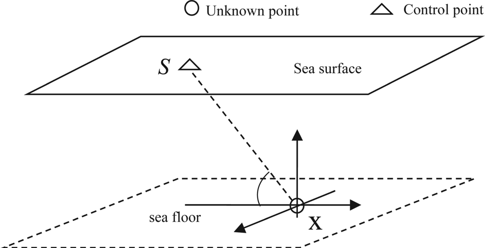
GNSS-A technology links GNSS and acoustic positioning methods to co-locate to accurately locate the position of the seafloor datum point. As shown in Figure 1, the transducer is installed under the ship and performs active ranging and positioning during the voyage, forming N sea-level dynamic control points within a period of time. Using GNSS technology can accurately determine their three-dimensional (3D) coordinates. When there are multiple distance observations, the 3D position information of the target point can be obtained through the distance intersection method (Sun, Reference Sun, W.2007). The underwater positioning observation model based on the average sound speed is:

where ${L^s}$ is the propagation distance of the acoustic signal from the sea surface transducer to the transponder; ${v^s}$
 is average sound speed; ${t^s}$
 is the propagation time; ${||{{\bf x} - {{\bf x}^s}} ||_2}$
 is the Euclidean distance between two points; ${\varepsilon _L}$
 is the equivalent ranging error; N represents the number of sea surface movement control points.
GNSS/acoustic positioning local coordinate system

Carry out the Taylor series expansion of Equation (1) at the initial value ${{\mathbf x}_0}$ to obtain the linearised equation:

where ${\mathbf dx} = {\mathbf x} - {{\mathbf x}_0}$ is coordinate correction number; ${r_i}$
 is the linearisation residual term, which can generally be ignored;

${{\mathbf e}_i}$ is the direction cosine. When there are three or more observations, the adjustment criterion is introduced, and the least square solution can be expressed as:

where ${\bf P}=\left[ {\begin{array}{*{20}{c}} {{{\bf P}_1}} & \ldots & {{{\bf P}_{\rm n}}} \end{array}} \right]$ is the observation weight matrix; ${\bf b = }\left[ {\begin{array}{*{20}{c}} {d{\boldsymbol{L}_1}} & {d{\boldsymbol{L}_2}} & \cdots & {d{\boldsymbol{L}_n}} \end{array}} \right]$
 ; ${\bf J}=\left[ {\begin{array}{*{20}{c}} {{\bf J^{\prime}}} & {{{\bf k}_n}} \end{array}} \right]$
 is called Jacobi matrix:

${\bf k}$ is the column matrix with a content of 1. Based on the initial value ${{\mathbf x}_0}$
 , the coordinates of the underwater point to be measured can be calculated iteratively:

From the range-finding underwater positioning model, we can see that the sound speed is the most important parameter, and the selection of the sound speed directly determines whether the positioning result is reliable. Therefore, a lot of research and analysis have been done on the sound speed correction method in order to improve the accuracy of sonar underwater positioning.
2.2 Description of average sound speed
In the underwater positioning model, the range is determined by the sound speed and the propagation time. Currently, the time measurement error is generally within 0·1 ms (Zhao et al., Reference Zhao, S., Wang, Z. and Liu, H.2018). Therefore, the key to improving the positioning accuracy lies in the determination of the sound speed. The equation of state of sea water (Cai et al., Reference Cai, Y. and Cheng, P.2012) is:

where $\rho$ is the density at a certain point i in seawater; p is the instantaneous sound pressure at the same point; v is the sound speed which can be expressed as:

The three influencing factors mainly change with the depth direction, so the sound speed can be roughly expressed as a function of water depth, and the relationship between them is expressed by the SSP. The SSP can be measured by CTD (conductivity, temperature, depth) or calculated according to the sound speed experience model. The water environment in the ocean is relatively complex, and temperature is the first factor that affects the sound speed. Generally, the sound speed of the surface layer and thermocline in the ocean changes significantly, while the temperature of the isothermal layer is relatively stable (Zhao et al., Reference Zhao, J and Liang, W2019). Seasonal temperature and flow field changes can cause instability of the SSP. Therefore, the SSP has significant temporal and spatial characteristics, and its changes are irregular. Studies have shown that the sensitivity of SSP mismatch to source positioning at different depths is different (Su et al., Reference Su, Ma, Song, Guo and Lu2015), so it is necessary to measure the SSP of this area at the same time during underwater positioning measurement (Li, Reference Li, S.2015).
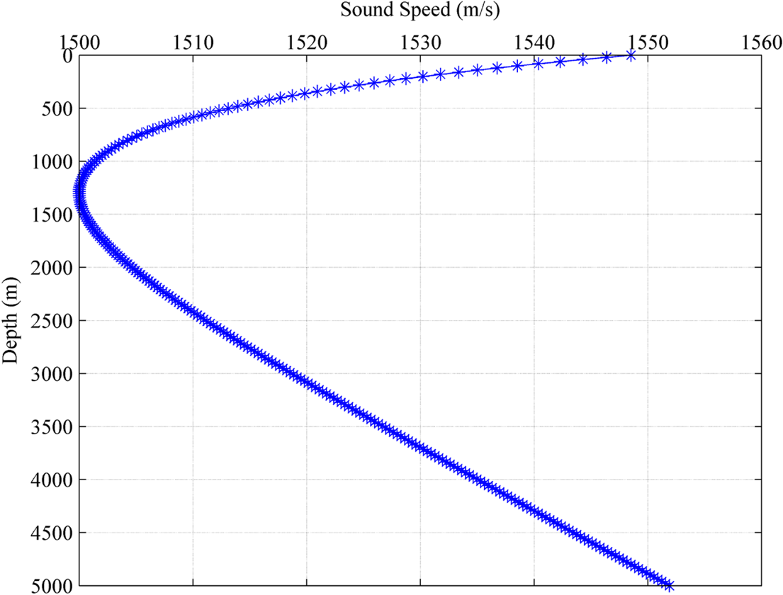
The classic ideal Munk-SSP (Figure 2) model is a parametric model of SSP structure. In the past few decades, it has been widely used in related research. It is a classic SSP model suitable for deep-sea areas based on the measured layered characteristics of deep-sea density structure. It is usually expressed by the function v(z) of sound speed v and water depth z (Munk, Reference Munk1974):

where $\kappa$ = 0·00737, conversion depth $\tilde{z} = {{2({z - 1300} )} / {1300}}$
 . When positioning without SSP, the Munk-SSP can be used as a simple replacement, or the global SSP can be constructed based on Argo data (Cai et al., Reference Cai, Cheng, Wen, Yang and Zhang2014).
Classic Munk sound speed profile

The premise of the positioning model based on distance measurement is that the sound speed is a constant, and the trajectory of acoustic rays in the water is a straight line. In order to improve the efficiency of underwater positioning in the project, based on experience, sometimes the sound speed value is directly taken as 1500 m/s. Obviously, this will bring a large ranging error. When the SSP is measured, the average sound speed based on the SSP is expressed as:

where H is the water depth, ${V_i}$ and ${V_{i + 1}}$
 are the sound speed values of the i and i+1 layer respectively, ${z_i}$
 and ${z_{i + 1}}$
 are the depths of the i and i+1 layer respectively. The positioning model of the average sound speed method is simple, the calculation method is convenient, and the positioning efficiency is high, but there is still a large residual error.
2.3 The effect of average sound speed on positioning
The acoustic ray, in practice, will bend due to the change of sound speed. Studies have shown that the sound speed determines the accuracy of positioning by affecting the accuracy of ranging. Based on the acoustic ray tracing algorithm, the relationship between ranging and surface sound speed error is derived (Zhao et al., Reference Zhao, J and Liang, W2019):

where k is Snell's constant, L is ranging, ${\theta _0}$ is the incident angle of surface acoustic rays, ${V_0}$
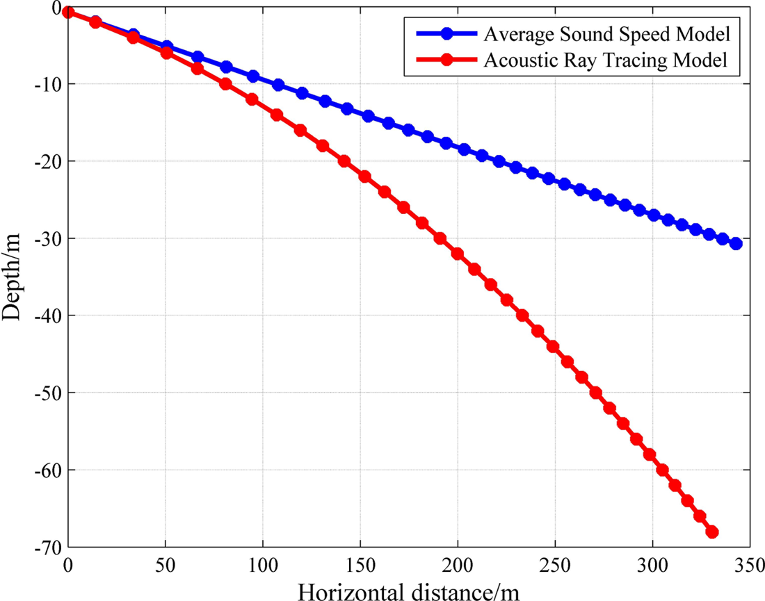
 is surface sound speed. It can be seen from Equation (11) that there is a non-linear relationship between the incident angle and the sound speed on the ranging, and the error of the sound speed and the incident angle are positively correlated with the ranging error. The acoustic ray tracing algorithm is a high-precision underwater positioning method commonly used to reduce the acoustic ray bending error (Sakic et al., Reference Sakic, Ballu, Crawford and Woeppelmann2018). When the observed incident angle is large, the average sound speed positioning model and acoustic ray tracing algorithms are used to calculate the horizontal distance of acoustic ray propagation at an incident angle of 85°, the average sound speed is 1470 m/s.
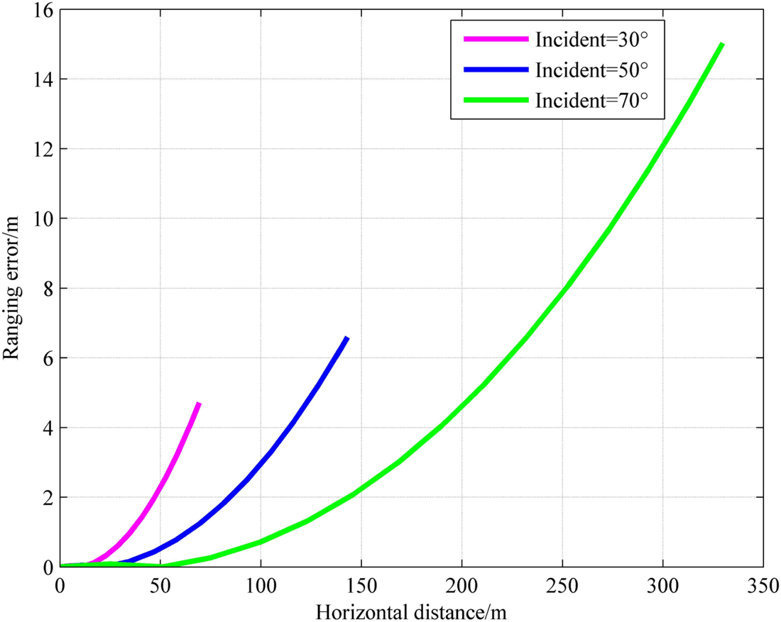
It can be seen from Figure 3 that, when the acoustic signal propagates to the horizontal distance of about 30 m, the difference between the two algorithms begins to appear. When the horizontal distance between the transponder and the source is close to 350 m, under the average sound speed model, the acoustic ray travels to 30 m underwater. While the acoustic ray travels to 70 m under the acoustic ray tracing algorithms, it has a significant impact. In addition, the influence of the average sound speed error on the ranging error under different incident angles is also calculated.
Influence of average sound speed error

In Figure 4, the sound source depth is 1 m, the incident angle is 30°, 50° and 70°, the average sound speed is 1,470 m/s, and the propagation time is 0·477 s. It can be seen from the experimental results that the horizontal distance reached by the signal propagation under different incident angles is different; The ranging error is affected by the acoustic ray bending error caused by the sound speed error, and it is positively correlated with the incident angle. When the transponder is directly below the sound source, there is no influence of acoustic ray bending error. In addition, the longer the sound signal propagation time, the greater the impact of the sound speed error. Assuming the propagation time is 1 s, the sound speed error of 1 m/s will result in a 1 m ranging error.
Effect of average sound speed error on ranging error

The acoustic ray tracing algorithm can effectively reduce the influence of the acoustic ray bending error and restore the footing of the beam more realistically. However, the calculation model of the algorithm is relatively complicated, and the calculation efficiency is lower than that of the average sound speed positioning model, and rapid positioning cannot be achieved. Therefore, it is necessary to consider sound speed correction to reduce the influence of the sound speed error. At present, the main sound speed correction methods include: empirical sound speed method, weighted average sound speed method, Taylor series expansion method, effective sound speed method, equivalent SSP method and acoustic ray tracing algorithm. Due to the limitation of the algorithm, the above method has many applicable conditions, and each has its advantages and disadvantages (Vincent and Hu, Reference Vincent and Hu2000; Nie, Reference Nie, Wang and Li2015; Zhang, Reference Zhang, B.2019).
It is easy to obtain from ray theory that when the depth of the target point to be measured is certain, the larger the incident angle, the longer the propagation distance. Therefore, an improved model of incident angle sound speed is considered. On the basis of the traditional average sound speed, the influence of incident angle error is considered, and the calculation complexity is simplified, so as to improve the positioning accuracy while ensuring the calculation efficiency.
3. A new average sound speed model for underwater positioning
Absolute calibration of submarine array is an important task of underwater positioning, which provides strong support for the construction of the submarine array network and the establishment of marine benchmarks (Wu, Reference Wu, Y.2013). In order to weaken the influence of incident angle error as much as possible, the method of circle calibration combined with tracing experiment is usually used to improve the positioning accuracy. Incident angle error includes the error caused by the change of sound speed, the control point error on the sea surface and the propagation time error.
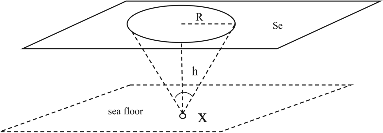
When the sea surface control pattern is a circle (Figure 5), a ‘star configuration’ has been proposed to eliminate the speed error caused by using different observations, to improve the accuracy of underwater positioning (Xue et al., Reference Xue, S., Dang, Y. and Zhang C.2006). Xue (Reference Xue, S. and Yang, Y.2014) proposed a nested cone configuration and a spiral configuration based on the minimum geometric dilution precision (GDOP) configuration for the expansion of the ‘star configuration’, and deduced the only five regular polyhedral configurations in mathematics. When the ship's trajectory is approximately circular, the incident angle information is approximately equal, so the influence of the error is minimised. In addition, due to the limited sailing distance of the ship, it can be approximately considered that the SSP used for positioning in a short time is the same. At this time, the influence of the incident angle error can be approximately ignored, and the distance between the shipborne transceiver and the seabed array element is regarded as a straight line, that is, the average sound speed can be used to achieve high-precision positioning (Qi et al., Reference Qi, Qu, Xue, Xu and Su2019).
Absolute calibration navigation positioning

Sometimes, however, limited by environmental conditions or positioning requirements in practice, the ship's trajectory on the sea surface is no longer a regular circular symmetrical figure. In this case, the propagation distance of the acoustic ray is different due to the different incident angle, and bending error cannot be ignored due to the influence of sound speed change. If a single sound speed is used, it will cause large positioning error and seriously affect the positioning accuracy. In conclusion, based on the classic Munk-SSP model, a sound speed function model related to the incident angle is established by numerical simulation experiments.
Assume that, under ideal conditions, a series of control points are distributed on a symmetric circle with R radius of the sea surface, and the plane position of the unknown point to be measured is located at the centre of the circle (as shown in Figure 5). Given the water depth of the unknown point to be measured, the incident angle can be calculated iteratively (Wang et al., Reference Wang, Li, Nie, Wang and Wu2016). The observed incident angle can be obtained by inverse calculation of the coordinates between the sea surface control point and the seabed point to be measured:

where $({x_i^s,y_i^s,z_i^s} )$ is the coordinates of the i control point on the sea surface, $({{x_{\rm x}}{y_{\rm x}}{z_{\rm x}}} )$
 is the coordinates of the point to be measured on the seabed.
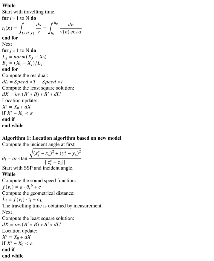
The acoustic ray tracing algorithm is used to simulate the sound signal propagation time t, the average sound speed v is calculated by Equation (10), and the sound speed is multiplied by the time to obtain the ranging for positioning. Keep changing until the best sound speed $v^{\prime}$ is found, so that the error between the positioning result ${\textrm{X}_{\rm v}}$
 and the ray tracing positioning result ${\textrm{X}_{\textrm{tracing}}}$
 meets the requirements, $||{{\textrm{X}_{\rm v}} - {\textrm{X}_{\textrm{tracing}}}} ||\le \varepsilon$
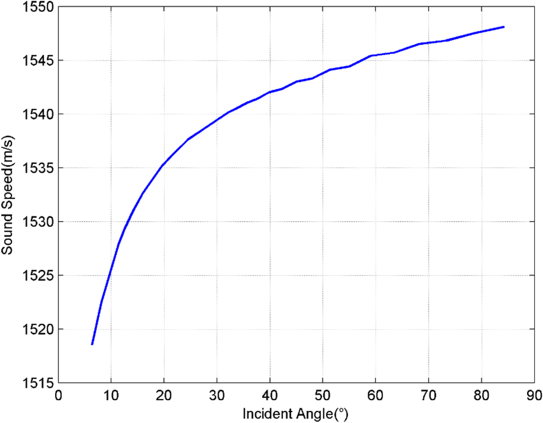
 . From this, the optimal sound speed value at a fixed incident angle can be obtained and then, by changing the water depth of the unknown point to be measured to control the incident angle transformation, the relationship between the incident angle and the optimal sound speed can be obtained, as shown in Figure 6. The step length of the incident angle is 2° and the interval is from 8° to 85°.
Relationship between incident angle and sound speed

At this time, the new sound speed positioning model related to the incident angle can be expressed as:

where $\tilde{L}$ is the slant distance; $\textrm{t}$
 is the propagation time of the acoustic signal; $f(v )$
 is a variable function of the sound speed; and the sound speed itself is a function of the incident angle, which can be obtained by fitting the function to Figure 6:

where a is the scaling factor adjustment factor; b is the constant dependent variable of the power function; c is the constant; $\theta$ is the incident angle. According to the numerical simulation test results, the value range of a is [−96·43, −93·29], the value range of b is [−0·4216, −0·3694], and the value range of c is [1562, −1566]. Among them, because the linear relationship between the incident angle and the sound speed is constant, the value range of a and b is unchanged. The premise of this experiment is the Munk-SSP model; there is a difference in the range of sound speed changes compared with different SSP, so the range of c depends on the SSP.
The sum of squares due to error (SSE) represents the sum of squares of errors between the fitted data and the corresponding points of the original data. The closer the SSE is to zero, the better the model selection and fitting, and the more successful the data prediction. The SSE of the model fitting function is 0·8501, indicating that the fitting result is very good. R-square is defined as the ratio of SSR (sum of squares of the regression) to SST (total sum of squares). The closer its value is to one, the stronger the explanatory power of the variables of the equation is for y, and the model fits the data better. The R-square of the fitting function is 0·9995, which can also prove that the fitting accuracy is very high.
When the angle of the acoustic ray connecting the sea surface transducer and the transponder to be measured is different, the n incident angles $\boldsymbol{\theta } = [{{\theta }_1},{{\theta }_2}, \cdots {{\theta }_n}]$ of the acoustic ray can be calculated by Equation (12). Then calculate n corresponding sound speed values $\textbf{v} = [{v_1},{v_2}, \cdots {v_n}]$
 through Equation (14). When the survey ship performs positioning measurement, it will output n acoustic ray propagation time $\textbf{T} = [{\textrm{t}_1},{\textrm{t}_2}, \cdots {\textrm{t}_n}]$
 can calculate the ranging $\textbf{L} = [{\textrm{L}_1},{\textrm{L}_2}, \cdots {\textrm{L}_n}]$
 . The symbol ‘L’ should be the observed value of multiple ranging, and this ranging refers to the distance between the transponder and the transducer. And then complete the positioning of the underwater target point to be measured according to the distance intersection method. Under this model, when the incident angle changes, the sound speed changes accordingly, which can effectively reduce the influence of the sound speed error on ranging. The above positioning process can be summarised as follows:
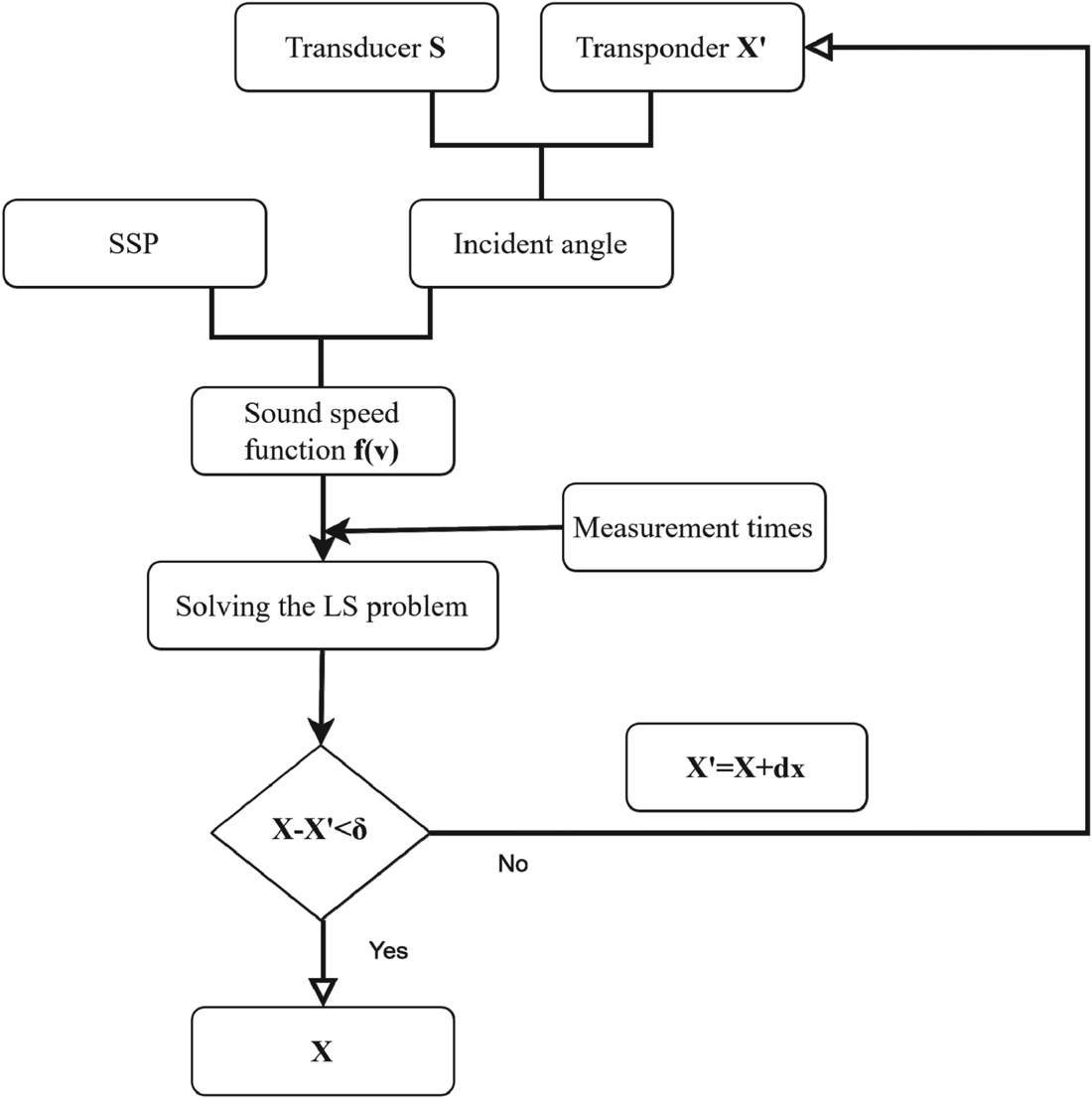
In the Figure 7, ‘X’ represents the coordinate position of the unknown point, and ‘$\mathrm{X^{\prime}}$ ’ represents the least squares solution obtained by using the positioning model proposed in this paper. The algorithm uses an iterative algorithm; when the positioning result does not meet the error requirements, the probability coordinates of the unknown point need to be changed to recalculate the angle of incidence. According to the relationship between the sound speed and the incident angle, a new value of sound speed is obtained, and the new unknown point coordinates are calculated. If $\textrm{X} - {{\rm X}^{\prime} < \delta }$
 , the iterative calculation ends, and the position coordinate ‘X’ obtained at this time is the true position of the underwater unknown point. The core idea of the new algorithm is given in the form of a program in the Appendix.
Positioning flowchart under the new model

4. Experiment analysis
4.1 Simulation experiment and analysis
The simulated trajectory of the ship on the sea surface is a circle with radius R = 100 m, the plane position of the unknown target point is at the centre of the circle, and the vertical position is 100 m underwater. Based on Munk-SSP, the ray tracing algorithm is used to simulate the propagation time of the acoustic signal. The simulated sea surface is a cosine wave with a wave height of 2 m, the measured ship speed is 3 kn/h, the sampling interval is 4 s, and the ranging error is 0·3% times the slope distance (Zhao et al., Reference Zhao, S., Wang, Z. and Liu, H.2018). The positions of the seafloor target in simulation test are known, so it is possible to compare the accuracy of positioning results of different models.
Three different sound speed determination methods are used for positioning experiments. The first model is the average sound speed of Munk-SSP, that is, ${\textrm{V}_{\rm 1}}\textrm{ = mean}[{\textrm{SSP(}\textrm{v}\textrm{)}} ]$ . The second model is based on the positioning results of the ray tracing algorithm, that is, ${\textrm{V}_2} = \textrm{tracing}(SSP)$
 . The core idea of the ray tracing algorithm is given in the form of a program in the Appendix. The third model is to use the new sound speed positioning model related to the incident angle ${\textrm{V}_3}({\theta } )$
 proposed in this paper; its calculation flow is shown in Figure 7. The positioning experiment was repeated 500 times, and the deviation sequence and variance of different positioning models and true values were counted to evaluate the reliability of the results.
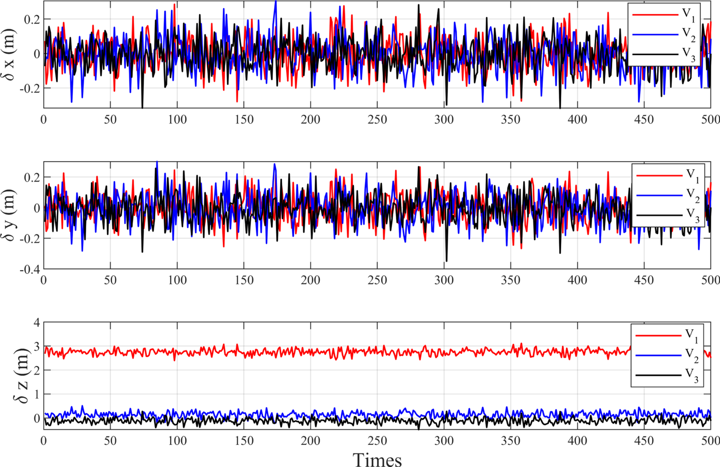
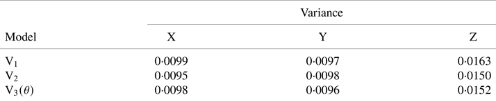
Several conclusions can be seen from the experimental results in Figure 8 and Table 1:
1. When the average sound speed model ${\textrm{V}_1}$
 is used for positioning, since the sea surface control graphic is a symmetrical circle, the positioning accuracy in the plane direction is high, and the error with the real position of the target is small. The positioning error of the average sound speed model is mainly reflected in the vertical direction, because the water surface control points are approximately coplanar, resulting in an ill state in the vertical direction, so the vertical positioning accuracy is poor.
2. When the ray tracing model ${\textrm{V}_2}$
is used for positioning, it can be seen that the positioning result is very close to the real position of the target. The reason is that the observation configuration is symmetrical, the incident angle is approximately equal, and the incident angle error affects the positioning accuracy through the ranging error.3. When the new positioning model ${\textrm{V}_3}({\theta } )$
is used for positioning, it can be seen that the deviation between the positioning result and the real position in the three directions is very small, and it is similar to the ray tracing model. The reason is that the sound speed used to calculate the distance measurement is no longer a single sound speed value, but a function related to the incident angle.4. Compared with the average sound speed positioning model, the new positioning model related to the incident angle improves the vertical positioning accuracy. Compared with the ray tracing model, the positioning accuracy is equivalent under the symmetrical circle control graph; when the sea surface control graphics is not a circularly symmetrical graph, the advantages of the new model will be reflected, and the authors will verify this conclusion in subsequent experiments.


Underwater geometric positioning errors caused by three sound velocity models under the same incident angle

Variance of positioning results under different models

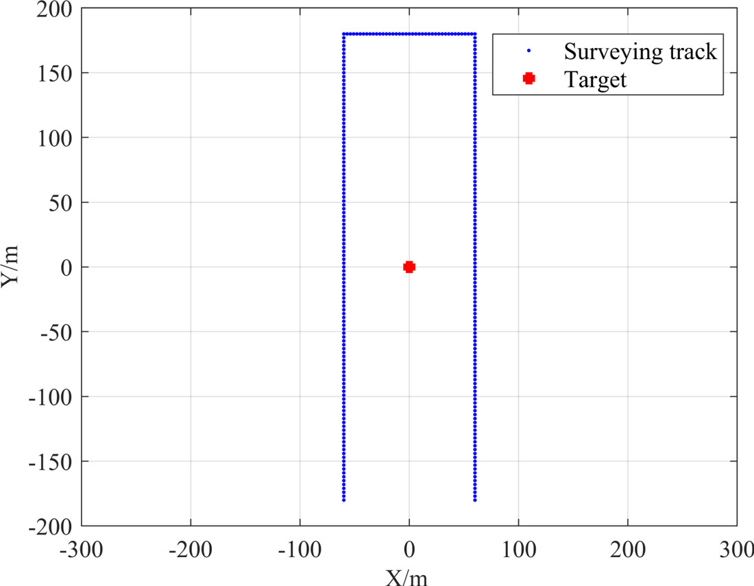
In addition, a simulation experiment was conducted with different incident angles. The surveying track of the simulated ship on the sea is a rectangle, and the error simulation method is the same as the above simulation experiment. The surveying track of the ship on the sea is shown in Figure 9, ‘Target’ indicates the position of the underwater target point.
Rectangular surveying track

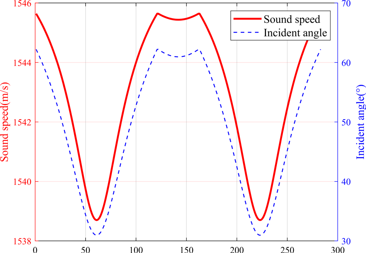
Correspondingly, according to the change of the incident angle, the corresponding sound speeds are calculated by Equation (14), and the relationship between them is shown in Figure 10.
Relationship between sound speed and incident angle

Similar to the above simulation experiment, three different positioning models are used for calculation. ${\textrm{V}_1}$ is the average sound speed positioning model, ${\textrm{V}_2}$
 is the ray tracing positioning model, and ${\textrm{V}_3}$
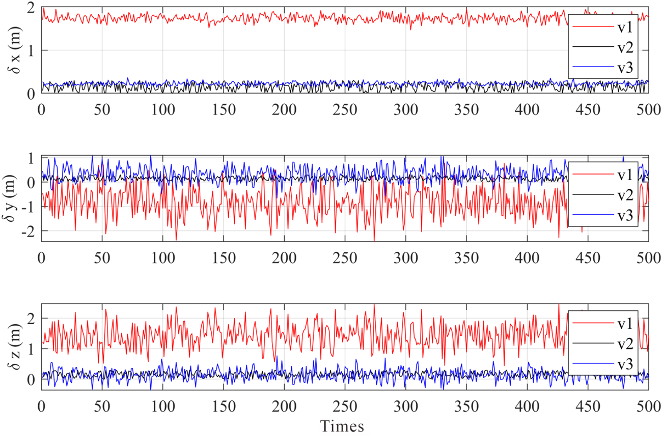
 is the new sound speed positioning model. The positioning error is shown in Figure 11.
Underwater geometric positioning errors caused by three sound velocity models under different incident angles

Through the experimental results, we can see that the ${\textrm{V}_1}$ model has poor positioning accuracy in three directions for the observations with the unequal incident angles. The reason is that a fixed sound speed is used for positioning. The positioning accuracy of the ${\textrm{V}_2}$
 and ${\textrm{V}_3}$
 models perform better than ${\textrm{V}_1}$
 , and the overall conclusion is the same as the above simulation test with the equivalently incident angles.
In summary, whether it is a circular calibration experiment or a positioning experiment with irregular observation patterns, the new positioning model related to the incident angle can quickly achieve high-precision underwater positioning.
4.2 Real experiment and analysis
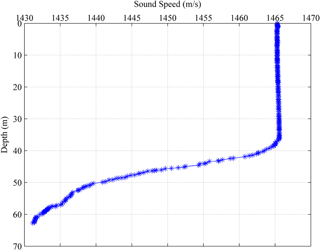
In order to verify the validity of the new positioning model related to the incident angle proposed in this paper, relevant actual measurement experiments were carried out. The positioning experiment was carried out in October 2012 on a lake in northern China, with a total area of about 554 km2 and maximum water depth of about 77 m. The target transponder was about 60 m underwater. The main equipment required for the experiment were: a measurement ship equipped with Leica GPS1200 dual-frequency real-time kinematic (RTK), vertical reference unit (VRU), Gyroscope (Gyro), long-base line (LBL) positioning system, sound velocity profile (SVP), data processing centre, etc. The LBL system used Sonardyne's 6G LBL acoustic positioning system. The ship's attitude sensor model was Seatex MRU-05, with roll/pitch measurement accuracy of ±0·05° and heave accuracy of ±5 cm. The underwater sound speed meter used AML SVP to measure the SSP of the water area Figure 12.
Sound speed profile of the survey area

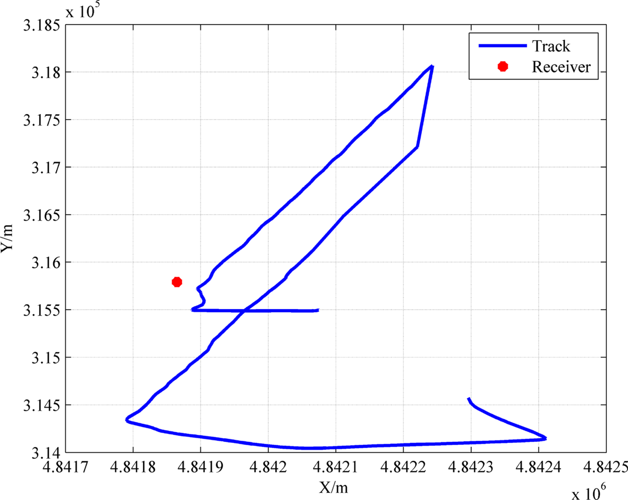
The experiment used track navigation and positioning, that is, the measuring ship did not follow a regular shape on the water surface, and the observation values at different incident angles were obtained. The sailing track is shown in Figure 13.
Survey ship's trajectory and the position of the receiver

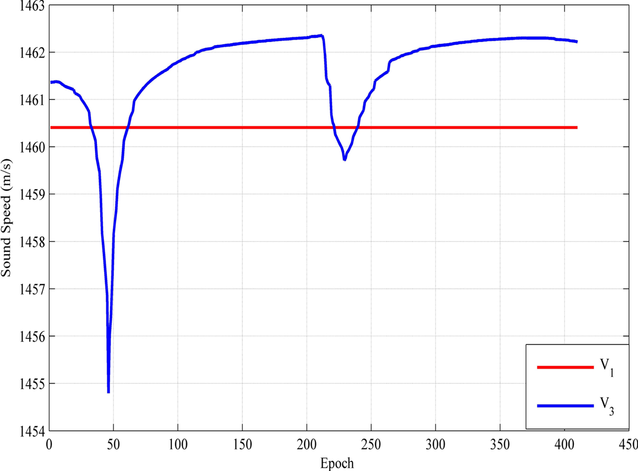
According to the initial value of the transponder position and the coordinates of the dynamic control point of the measuring ship, the incident angles of different observations can be inversely calculated, and then the new sound speed positioning model ${\textrm{V}_3}({\theta } )$ can be calculated by Equation (14); at the same time we give the average sound speed ${\textrm{V}_1}$
 . Figure 14 shows the comparison of the relationship between the two sound speed values.
Comparison of two sound speeds

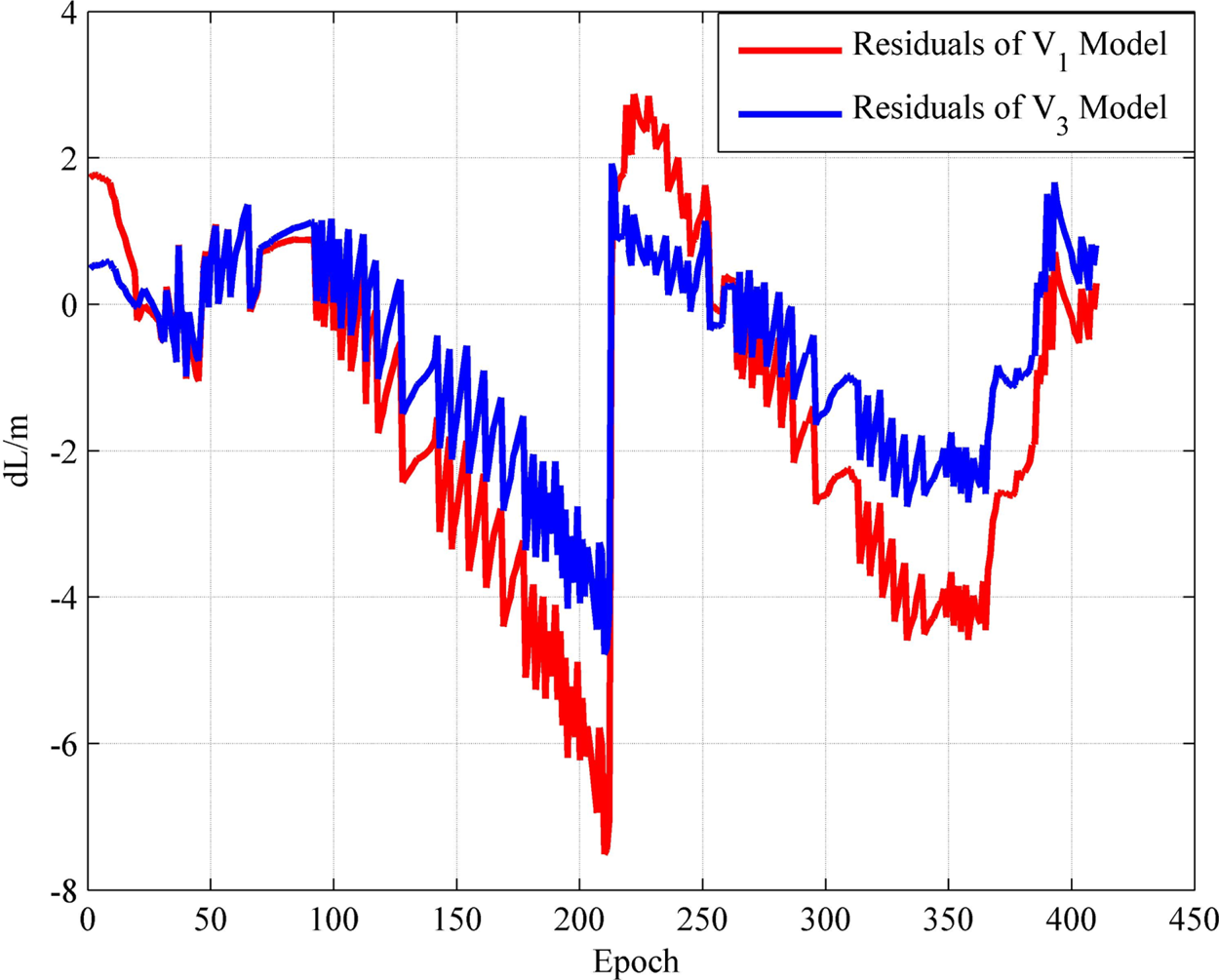
Positioning results were performed under two different models. The residual information contains important information about the basic assumptions of the model, and the residual relationship under the two positioning results is given (Figure 15).
Comparison of residuals of two positioning results under two models

It can be seen from the positioning residuals of the two positioning models that the residuals of the new sound speed positioning model ${\textrm{V}_3}({\theta } )$ are generally smaller than the average sound speed positioning model ${\textrm{V}_1}$
 . The reason is that the ${\textrm{V}_3}({\theta } )$
 is used instead of a single sound speed value ${\textrm{V}_1}$
 , which releases the residual information, reduces the influence of the sound speed error on the positioning, and improves the accuracy of parameter estimation.
In addition, it was noticed that there is a significant mutation for positioning residuals approximately at the 210th epoch. Combined with the navigation route in Figure 12, and through the position relationship between the transducer and the underwater transponder, the authors believe that at the 210th epoch the ship sailed to the farthest point, and then the route and direction of sailing changed, where the incident angle and other related errors have the greatest impact.
Taking the acoustic ray tracing positioning result as the true value, Table 2 shows the deviation of the positioning results in three directions under different models. From the results, the results of the ${\textrm{V}_3}({\theta } )$ model in the three directions are closer to the results of acoustic ray tracing, and the positioning accuracy has been greatly improved. The three directions of X, Y, and Z are raised by about 3 m, 0·8 m and 2·4 m, respectively. From the positional error (PE) value, $\textrm{PE = }\sqrt {{{\mathrm{(\Delta X)}}^2} + {{\mathrm{(\Delta Y)}}^2} + {{\mathrm{(\Delta Z)}}^2}}$
 , the PE values under the two models are 4·9848 and 1·1233, respectively. It is obvious that the ${\textrm{V}_3}({\theta } )$
 model is effective.
Deviation of positioning results under different models: unit (m)

5. Conclusion
Based on the introduction of the average sound speed positioning model, this paper discusses the influence of sound speed error on positioning accuracy. Combined with the actual situation, considering the influence of the error related to the incident angle, a new sound speed positioning model related to the incident angle is established to replace the single sound speed value in the average sound speed model for positioning. The following conclusions were obtained through simulation experiments and actual measurement experiments:
(1) The error of sound speed is an important source which affects the accuracy of underwater positioning and cannot be ignored. Sound speed error affects the ranging and causes the positioning result to be inaccurate. Therefore sound speed correction is required for high-precision underwater positioning.
(2) Considering the impact of incident angle related errors on positioning, this paper proposes a new sound speed positioning model related to the incident angle to reduce the model error. Through experiments, the average sound speed model has a large positioning error due to the incident angle error, especially in deep water and long-distance positioning. The new sound speed positioning model related to the incident angle proposed in this paper is used for positioning, and it shows good positioning performance when the observation graph is circular or non-circular.
(3) The starting point of the new positioning model proposed in this paper is to fit a positioning model with a small number of acoustic rays. Once the model is established, when the user performs repeated positioning in a certain area, it does not need to repeat the complicated acoustic ray tracing positioning calculations, but only needs to calculate a correction value according to the new model, and the positioning can be realised quickly based on this correction value. It can reduce the cost of calculation on the basis of ensuring the positioning accuracy, which is convenient for users.
Funding statement
This study was supported by the National Natural Science Foundation of China (No. 41931076), Major Science and Technology Innovation Projects of Shandong Province (No. 2019JZZY010809).
APPENDIX
Ray tracing algorithm