I. INTRODUCTION
Wide range of engineering parts require specific treatment to improve their mechanical and/or corrosion resistance to enhance the fatigue (life), as well as the deformation resistance. For such purposes, shot peening is one of the favorite candidates. The principle of this process is to impact the metallic surface to be treated using small steel balls that create plastic strain, improve hardness, induce compressive residual stress, and increase the fatigue strength. Reference Abramov, Abramov, Sommer, Gradov and Smirnov1
To better control and predict this well-known process, finite elements method (FEM) simulation of multiple impacts has been developed, Reference Miao, Demers, Larose, Perron and Lévesque2–Reference Mylonas and Labeas4 but the accuracy of such model is limited by the use of pertinent stress–strain behavior laws. Johnson–Cook [Eq. (1)] or Hollomon's [Eq. (2)] laws are generally introduced into the models, but determining the correct values of the material parameters is a great challenge.
 $$\sigma = \left( {A + B{{\left( {{\varepsilon ^{\rm{p}}}} \right)}^n}} \right)\left( {1 + C\ln \left( {{{{{\dot \varepsilon }^{\rm{p}}}} \over {{\varepsilon _0}}}} \right)} \right)\left( {1 - {T^{{\rm{*}}m}}} \right)\quad ,$$
where εp is the equivalent plastic strain, A is the yield strength,
 ${{{{\dot \varepsilon }^{\rm{p}}}} \mathord{\left/ {\vphantom {{{{\dot \varepsilon }^{\rm{p}}}} {{\varepsilon _0}}}} \right. \kern-\nulldelimiterspace} {{\varepsilon _0}}}$
is the normalized plastic strain rate for ε0 = 1.0/s, n is the hardening exponent, C is the strain rate sensibility coefficient, T* is the homologous temperature, and B and m are constants.
 $$\sigma = k{\varepsilon ^n}\quad ,$$
where k is the strength coefficient, and n is the strain hardening exponent.
Considering the dynamic aspect of shot peening, dynamic impact tests, such as split Hopkinson pressure bars (SHBP), may be performed to obtain the dynamic behavior law and, therefore, the material parameter, Reference Jaspers and Dautzenberg5 but these techniques can only reflect the bulk behavior of the tested materials and cannot take into account the specific surface behavior that may be predominant during shot peening tests. Other authors identify the local behavior by quasi-static instrumented indentations. Reference Beghini, Bertini and Fontanari6–Reference Collin, Mauvoisin, Pilvin and El Abdi8 If such methods enhance surface effects, static conditions cannot reveal the dynamic effect of shot peening. To combine the dynamic effect and microscale analyses, a microimpact testing apparatus was developed and instrumented where 2 mm diameter balls are punched into the sample surface at controlled energy. Reference Kermouche, Grange and Langlade9,Reference Lamri, Langlade and Kermouche10 This experimental setup enables to perform repeated impacts at the same point and, therefore, to follow the progressive plastic deformation that may be induced by the cyclic loadings. In parallel to the experimental work, an inverse method was developed to obtain the stress–strain curve of metallic materials from the experimental results. In accordance with many other authors, Reference Beghini, Bertini and Fontanari6,Reference Dao, Chollacoop, Van Vliet, Venkatesh and Suresh11,Reference Huang, Liu, Zhou, Ma and Lu12 Hollomon's law has been chosen to describe the usual behavior of the tested metals. In addition to the inverse method, an analytical approach has been used to obtain an estimation of the stress–strain curve. The use of this second method aims at testing the validity of the inverse identification and increasing the confidence in the obtained results. These two methods have been described and validated using virtual and real, but ideal material, i.e., commercially pure copper. Reference Al Baida, Kermouche and Langlade13 In the previous work, Reference Al Baida, Kermouche and Langlade13 the inverse method was tested in a strain range between 0.6 and 0.8, and information about the low strain range was missing because only 2 mm diameter balls were used resulting in a reduced strain field. In the present paper, dynamic tests have been performed with balls of different sizes to obtain lower strain values and collect more experimental data. Besides, this study also presents applications of both the inverse method and the analytical approach to several industrial materials.
II. THE MICROIMPACT MACHINE
The microimpact machine is based on a micromarking machine that has been modified to project balls with controlled speed and position. This machine is equipped with a force and a displacement sensor connected to a complete acquisition chain, which allows to obtain the impact speed, i.e., the impact energy, as well as the induced force as a function of time during each single impact. By adjusting the pulse duration in the electromagnet and initial impactor position, the impact speed can vary from 100 to 600 mm/s, which corresponds to an impact energy ranging from 1 to 31 mJ. New ball holders have been developed to allow the microimpactor to project balls from 2 to 20 mm diameter. The microimpactor can be used in dynamic regime as well as under static condition by manually punching the ball onto the sample surface following the standard Brinell hardness procedure. The Eq. (3) shows that the strain ε is inversely proportional to R (the radius of the ball) and a (the radius of the residual imprint). According to this equation, 1 mm radius balls allow to achieve the highest deformation domain, whereas 5 and 3 mm radius balls induce low deformation.
 $$\varepsilon = 0.2{a \over R}\quad .$$
III. THE FINITE ELEMENT MODEL
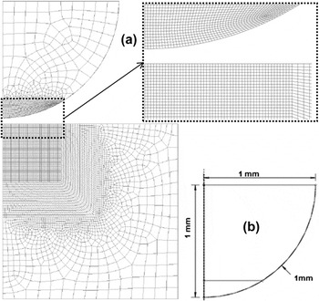
The objective of the FEM simulation is to obtain the impact load and the radius of the residual imprint after 10 impacts at a given energy to develop databases that will be used in the inverse method. Repeated impacts were modeled with a finite element model developed in ABAQUS-Explicit. 14 This model was already described in a previous work. Reference Al Baida, Kermouche and Langlade13 Figure 1 shows the FEM model, the substrate is considered as semi-infinite solid with a behavior law related to k and n Hollomon parameters, and the ball is a 1 mm radius deformable elastic solid. To validate this model, the simulated load signal was compared with the experimental load signal and the calculated force value Reference Johnson15 under pure elastic conditions. A typical error of 9% has been observed on M2 treated samples. Reference Al Baida, Kermouche and Langlade13
FEM model for simulating the impact test: (a) complete model and (b) ball dimension.

The same databases presented in Al Baida et al. Reference Al Baida, Kermouche and Langlade13 have been used in the present study.
IV. THE ANALYTICAL APPROACH
Based on Tabor, Johnson and Hill, Reference Johnson15–Reference Tabor17 Kermouche et al. Reference Kermouche, Loubet and Bergheau18 presented a direct method to estimate the local stress–strain curve of materials under sharp indentation test. This method has already been described in the case of spherical indentation in Al Baida et al. Reference Al Baida, Kermouche and Langlade13 and validated by blind tests on virtual materials and real tests on pure copper. Based on the mean pressure, the radius of residual imprint, and the elastic properties of the tested materials, stress–strain values can be obtained.
The analytical equations of stress and strain can be written as follows:
 $${\sigma _{\rm{r}}} = {{\zeta {a \over R}{P_{\rm{m}}}} \over {{\gamma _{\rm{p}}}\zeta {a \over R} - \left( {1 - \zeta B} \right){{{P_{\rm{m}}}} \over E}}}\quad ,$$
 $${\varepsilon _{\rm{r}}} = \left( {1 - \zeta B} \right){{{\sigma _{\rm{r}}}} \over E} + \zeta {a \over R}\quad .$$
In the previous expression [Eq. (4)], the mean pressure can be written as: P m = L/πa 2, where L is the applied load, and a is the contact radius. The value of γp has been fixed equal to 2.8, as suggested by Tabor. Reference Tabor17 The value of B is equal to (1 − ν2)*(3.3*π/4) and ζ is given by the following equation:
 $$\zeta = {4 \over {3\pi {\gamma _{\rm{p}}}\left( {1 - {\nu ^2}} \right)}}\quad .$$
R is linked to the indenter geometry, so this value is known. The elastic properties of the materials being also known, the value of B and ζ can be deduced. Considering the experimental values obtained for load and radius, P m can be calculated and the stress–strain values for the tested materials can be determined. However, the main advantage of the analytical approach is that it can provide data on the behavior of materials in both low and high-strain range using different ball sizes.
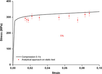
The efficiency of the analytical approach was tested during sharp indentations in Kermouche et al. Reference Kermouche, Loubet and Bergheau18 Figure 2 shows a comparison between the analytical approach using the spherical indentation and the static compression test of pure copper. A good correlation between analytical approach results and the static curve can be observed. If the yield stress of the tested materials cannot be identified using the analytical approach, the plastic deformation regime is well described.
Comparison between stress–strain curve of commercially pure copper under static compression and stress strain values obtained from analytical approach.

A. Blind tests on analytical approach
As the efficiency of the analytical approach was validated under static conditions, the next step is to determine the accuracy of the analytical approach under dynamic impacts. For that purpose, blind tests were conducted using virtual materials assumed to be following Hollomon's law.
Virtual materials have been tested with different values of k and n for 8 mJ impact energy. The elastic properties have been chosen as E = 210 GPa and ν = 0.3. The parameters k and n are as follows:
k:(800; 1500; 2800; 3300) MPa,
n:(0.12; 0.25; 0.35; 0.47).
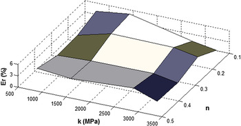
Figure 3 presents the relative error [Eq. (7)] during N = 10 impacts between the Hollomon original stress f o(ε) [Eq. (2)] and the predicted stress f p(ε) obtained by the analytical approach [Eq. (4)].
 $${E_{\rm{r}}} = 100{{\sqrt {\int_{{\varepsilon _1}}^{{\varepsilon _N}} {{{\left[ {{f_{\rm{o}}}\left( \varepsilon \right) - {f_{\rm{p}}}\left( \varepsilon \right)} \right]}^2}{\rm{d}}\varepsilon } } } \over {\sqrt {\int_{{\varepsilon _1}}^{{\varepsilon _N}} {{{\left[ {{f_{\rm{o}}}\left( \varepsilon \right)} \right]}^2}{\rm{d}}\varepsilon } } }}\quad .$$
Relative error E r of Eq. (7) as function of k and n, impact energy was 8 mJ.

Figure 3 shows that the error does not exceed 6%.
The error shows that the analytical approach allows to propose a good estimation of the stress–strain values using dynamic impact. These results then validate the use of the analytical method under dynamic impact conditions.
V. THE INVERSE METHOD
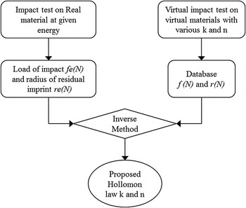
The inverse method has been developed by Kermouche et al. Reference Kermouche, Grange and Langlade9 to identify the local stress–strain curve using dynamic impact tests. This method was first based on the comparison between experimental results of radius and depth of residual imprints, and their corresponding values obtained from FEM simulations with several k and n parameters of the Hollomon's law (σ = kε n ). The method and associated databases have been developed for several impact energies. The inverse method identifies the values of k and n, which allow to reach the best approach between the experimental results and those of the FEM simulation. Figure 4 represents the general principle of the inverse method.
Flow diagram explaining the identification of the stress–strain curve using inverse method.

Referring to Kermouche et al., Reference Kermouche, Grange and Langlade9 the evolution of the load and radius values as a function of the number of impacts (N = 1–10) can be described by the following equation:
 $$x\left( N \right) = {A_x}\ln {\left( N \right)^2} + {B_x}\ln \left( N \right) + {C_x}\quad ,$$
where N is the number of impacts, x is the characteristic parameter of the impact, i.e., radius r and/or load f. As the simulations have been done for an already known impact energy, A x , B x , and C x are functions of (k and n) couple and describe the global evolution of x, they are stored in 2 databases, one for the radius (A r , B r , and C r ) and one for the load (A l , B l , C l ).
The experimental values of the radius of residual imprint and impact load after N impacts for a given energy can be noted re (N) and fe (N), whereas r(N) and f(N) are the radius and load values resulting from the FEM simulation.
Considering the experimental curves re (N) and fe (N) and the curves of FEM simulation r(N) and f(N), an identification method was developed to seek the minimal gap between the experimental and numerical curves and propose the best couple of k and n parameters of the constitutive law. This optimization method is based on the following equation:
 $${\rm{Minimum}}\left[ {{I_x}\left( {k,n} \right) = 100{{\sqrt {\int_0^{N\,\max } {{{\left( {x - {x_{\exp }}} \right)}^2}{\rm{d}}N} } } \over {\sqrt {\int_0^{N\,\max } {{{(x)}^2}{\rm{d}}N} } }}} \right]\quad .$$
If the accuracy of this method has been already validated by blind tests on virtual materials and through real tests on ideal materials like pure copper, Reference Al Baida, Kermouche and Langlade13 its use and pertinence have still to be demonstrated on industrial materials and compared with other experimental tests.
VI. EXPERIMENTAL TESTING
Ten successive dynamic impacts at controlled energies have been performed using zirconia balls ranging from 2 to 10 mm diameter and 6 mm diameter 100Cr6 ball. The inverse method was applied on the results of impact load and radii of the residual imprints after ten dynamic impacts using 2 mm diameter ball to identify a constitutive law. The analytical approach has been applied on all impact results and compared with the inverse method results. To assess the dynamic effect, the inverse method and analytical approach results are compared with the stress–strain curve of compression test or static traction test.
Based on Mok, Reference Mok19 the strain rate was estimated from Eq. (10).
 $$\dot \varepsilon = 0.2{v \over a}\quad ,$$
where v is the impact velocity and a the scar radius.
In this study, tested materials are pure copper, pure iron, and aluminum 6061-T651.
A. Application on pure copper
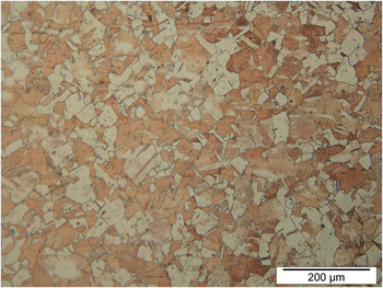
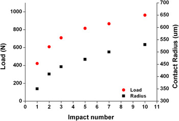
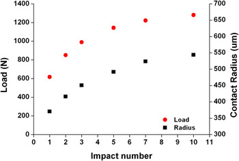
Commercially pure copper samples have been chosen for the first tests. As shown in Fig. 5, the microstructure consists of fine equiaxed grains involving an isotropic material behavior. Figure 6 shows the evolution of radius and load during 10 successive impacts for 11 mJ using 2 mm diameter balls.
Grain size of commercially pure copper.

Evolution of the radius (resp. load) on commercially pure copper as a function of the number of impacts using an impact energy of 11 mJ and a 2 mm diameter ball.

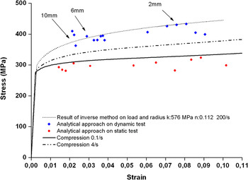
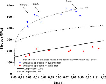
Figure 7 summarizes the different results obtained on copper samples. 2 compression curves are plotted for 2 different strain rates, i.e., 0.1 and 4 s−1. They clearly illustrate the influence of the strain rate showing that increasing the strain rate leads to a shift of the curve to higher stress levels. The analytical method has then been applied on static indentation results, and the corresponding points (red points) are plotted in Fig. 7, showing a quite good agreement with the static compression test (0.1 s−1). This confirms the pertinence of the analytical method for identifying static stress–strain curves from static spherical indentation. It also suggests that the strain rate imposed during spherical indentation may be slightly lower than 0.1 s−1. The Analytical method has also been applied on dynamic impacts obtained using 3 different ball types leading to a second set of points (blue points) on Fig. 7. Then the inverse method was launched on the 2 mm ball impacts to propose a dynamic stress–strain curve. The analytical points and the stress–strain law proposed through the inverse method are quite similar. These results confirm the influence of the strain rate on the stress–strain curve.
Comparison between stress–strain curves obtained by compression test at two strain rates on commercially pure copper, the result of the inverse method, and the result of the analytical approach in dynamic and static case using 2, 6, and 10 mm diameter ball sizes.

Considering the classical Johnson Cook equation [Eq. (1)], a strain rate sensibility coefficient of C = 0.038 may be deduced from the compression curve at 4 s−1 and the dynamic impact stress–strain curve using Eq. (11). It can be noted that in the case of OFHC copper, the value of C = 0.025 can be found in the literature. Reference Johnson and Cook20–Reference Peng, Zhong, Lu, Narayanan, Zhu and Lou22
 $$C = {{\left( {{\sigma _1} - {\sigma _2}} \right)} \over {{\sigma _2}\ln {{\dot \varepsilon }_1} - {\sigma _1}\ln {{\dot \varepsilon }_2}}}\quad .$$
B. Application on pure iron
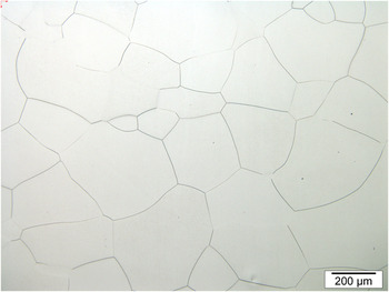
To test the efficiency of the inverse method, pure Iron BCC substrate (99:9997% iron) cylinders of 11 mm diameter and 5 mm thick obtained by cold crucible melting Reference Lacaille, Kermouche, Spinel, Feulvarch, Morel and Bergheau23 have been chosen. The mean grain size at 280 µm can be observed in the microstructure picture (Fig. 8). Figure 9 shows the evolution of impact radius and induced load on pure iron samples as a function of the number of impacts at 17 mJ using a 2 mm diameter ball. These values have then been used as input data for the inverse method (Fig. 4). Figure 10 summarizes the results of compression tests at two different strain rates, the result of the inverse method and the result of the analytical approach using ball size 2, 6, and 10 mm of diameter. It can first be noted that the analytical approach is in good agreement with the results of the inverse method. Moreover, according to Fig. 10, a large gap of 60% can be observed between the two compression curves obtained at different strain rates, demonstrating the high sensitivity of iron to the strain rate. Reference Ostwaldt, Klepaczko and Klimanek24 The analytical method has also been applied on dynamic and static impacts using the 3 different diameter ball sizes. The inverse method using the 2 mm ball impacts enables to propose a dynamic stress–strain curve. The stress–strain law proposed through the inverse method fits the analytical points with a reasonable agreement and confirms the influence of the strain rate on the stress–strain curve. Considering the compression curve at 4 s−1, the dynamic impact stress–strain curve and Eq. (11), a strain rate sensibility coefficient of C = 0.11 may be determined. Reference values of C = 0.06 may be found in the literature for Armco pure iron. Reference Johnson and Cook20 Higher values are noted for carbon or tool steels.
Microstructure of pure iron.

Growth of radius (load) on pure iron with the number of impact for impact energy of 17 mJ using a 2 mm diameter ball.

Comparison between the stress–strain curves obtained by compression test at two strain rates on pure iron, results of the inverse method, and results of the analytical approach in dynamic and static case using 2, 6, and 10 mm diameter ball sizes.

C. Application on aluminum (6061-T651)
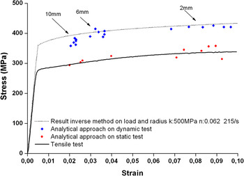
Similarly to the tests performed on copper and iron, the inverse method has been applied on Aluminum 6061-T651 at 10 mJ, the same inverse method result has been presented in a recent study. Reference Al Baida, Langlade, Kermouche and Ambriz25 Both analytical and inverse methods have been used to identify the stress–strain curve of this industrial material. The results have been compared with quasi-static traction tests performed at CIITEC-IPN in Mexico. Reference Ambriz, Froustey and Mesmacque26 Figure 11 confirms the good correlation between the analytical approach and the result of the inverse method and/or the tensile test. These results show that the proposed methods are also suitable for industrial materials likely to have heterogeneities. Despite the nonideal microstructure, the two methods can be used with a limited variability leading to the determination of a dynamic stress–strain curve. Regarding iron and copper, a shift toward higher stresses clearly appears with a higher yield stress about 30%.
Comparison between the tensile test on aluminum 6061-T651, inverse method, and analytical approach (using 2, 6, and 10 mm diameter ball sizes).

VII. CONCLUSION
This study presents an application of an inverse method to identify the stress–strain curve of materials subjected to high speed impacts like those occurring during the shot peening process. The inverse method was presented in Al Baida et al., Reference Al Baida, Kermouche and Langlade13 and it was validated by blind tests on virtual materials and by experimental results on commercially pure copper. This present work presents new applications on ideal materials like pure iron or commercially pure copper but also on an industrial aluminum 6061-T651. It also presents a comparison between the inverse method results and a direct analytical approach. This direct approach being only established for static sharp tip indentation, this work enables to state its validity for both static and dynamic spherical indentation. The results obtained for the three ideal and industrial materials show a good correlation between the inverse method and the analytical approach results. Numerical blind tests enable to estimate its accuracy and show that an approximate stress–strain curve of the materials within a 15% margin of error may be expected (estimate on virtual materials).
When a static traction or compression curve is available, the dynamic impact method also permits to give an estimation of the strain rate sensibility coefficient of Johnson Cook equation.
As this technique does not require large volumes of material or specific samples, its use may be a promising method to obtain static and dynamic stress–strain curves of all kinds of materials. Furthermore, considering the small volume of the impacted zone, it can be sensitive to surface treatment effects (shot peening, nitriding, coatings, welding, etc.), i.e., domains that are difficult to characterize using conventional techniques.
ACKNOWLEDGMENT
The authors gratefully acknowledge financial support from UTBM and the international relations that allocated funds for Mr. RR Ambriz as a visiting professor. They also wish to thank Mr. D. Schlegel and Mr. Th. Couturier for their help in the design and implementation of various indenter-holders and Mr. D. Tumbajoy for his help in the sample preparation and compression tests on pure iron and pure copper.