1. Introduction
The Richtmyer–Meshkov instability (RMI) arises when a perturbed interface separating two substances of different densities is impulsively accelerated by shock waves. This phenomenon was first theoretically predicted by Richtmyer (Reference Richtmyer1960) and later experimentally confirmed by Meshkov (Reference Meshkov1969). The RMI has attracted considerable attention over the past several decades (Zhou Reference Zhou2017a
,Reference Zhou
b
, Reference Zhou2024; Zhou et al. Reference Zhou2019, Reference Zhou2021) due to its crucial role in numerous significant engineering and scientific applications, particularly in inertial confinement fusion (ICF) (Nuckolls et al. Reference Nuckolls, Wood, Thiessen and Zimmerman1972; Lindl, McCrory & Campbell Reference Lindl, McCrory and Campbell1992; Betti & Hurricane Reference Betti and Hurricane2016; Zylstra et al. Reference Zylstra2022; Zhou, Sadler & Hurricane Reference Zhou, Sadler and Hurricane2025). In ICF, interface perturbations arising from manufacturing imperfections and material inhomogeneities are initially amplified during the early-time shock transit stage by RMI, which in turn seeds the significant growth of the Rayleigh–Taylor instability (Rayleigh Reference Rayleigh1883; Taylor Reference Taylor1950) occurring in the deceleration phase. These hydrodynamic instabilities can ultimately lead to violent mixing between ablator material and deuterium-tritium fuel, thereby hindering the achievement of high-energy-gain ignition Zhou et al. (Reference Zhou, Sadler and Hurricane2025). Presently, extensive research has been conducted on RMI at a once-shocked interface (Zhou Reference Zhou2024), revealing its sensitivity to initial conditions such as perturbation amplitude (Rikanati et al. Reference Rikanati, Oron, Sadot and Shvarts2003; Wang et al. Reference Wang, Wang, Zhai and Luo2023a
), shock intensity (Holmes et al. Reference Holmes, Dimonte, Fryxell, Gittings, Grove, Schneider, Sharp, Velikovich, Weaver and Zhang1999; Si et al. Reference Si, Jiang, Cai, Wang and Luo2025) and Atwood number (
 $A=(\rho _{{d}}-\rho _{{u}})/(\rho _{{d}}+\rho _{{u}})$
, where
 $\rho _{{d}}$
and
 $\rho _{{u}}$
represent the densities of substances downstream and upstream of the interface, respectively) (Dimonte & Ramaprabhu Reference Dimonte and Ramaprabhu2010; Chen et al. Reference Chen, Xing, Wang, Zhai and Luo2023; Xing et al. Reference Xing, Chen, Li, Wang, Zhai and Luo2025). Notably, in both conventional direct- and indirect-drive ignition schemes of ICF (Goncharov et al. Reference Goncharov, Knauer, McKenty, Radha, Sangster, Skupsky, Betti, McCrory and Meyerhofer2003; Lindl et al. Reference Lindl, Amendt, Berger, Glendinning, Glenzer, Haan, Kauffman, Landen and Suter2004), as well as in most innovative ignition schemes (Tabak et al. Reference Tabak, Hammer, Glinsky, Kruer, Wilks, Woodworth, Campbell, Perry and Mason1994; Murakami et al. Reference Murakami, Nagatomo, Azechi, Ogando, Perlado and Eliezer2006; Betti et al. Reference Betti, Zhou, Anderson, Perkins, Theobald and Solodov2007; Zhang et al. Reference Zhang2020), a multi-co-propagating-shock drive strategy is commonly employed to achieve the high drive pressure required for ignition while maintaining the target shell at a relatively low entropy. Therefore, investigating the evolution of RMI induced by two co-propagating shock waves (hereafter referred to as ‘S-RMI’) and exploring strategies to suppress its growth are critical for achieving sustainable fusion energy via ICF.
Under the assumption of incompressibility, which implies that
 $A$
remains unchanged during the first and second shock–interface interactions, Mikaelian (Reference Mikaelian1985) proposed that a second shock impact from the same side, hereafter referred to as ‘same-side reshock’, can only promote the instability at a light–heavy interface where
 $\rho _{{u}} \lt \rho _{{d}}$
and
 $A \gt 0$
. In contrast, at a heavy–light interface where
 $\rho _{{u}} \gt \rho _{{d}}$
and
 $A \lt 0$
, a same-side reshock can promote, suppress or even freeze the RMI evolution. Additionally, heavy–light interfaces are more commonly encountered than light–heavy interfaces in various types of ICF targets. Therefore, the present study focuses on S-RMI at heavy–light interfaces. Theoretically, Mikaelian (Reference Mikaelian1985) identified thirteen distinct perturbation evolution patterns in an incompressible two-shock system, and proposed a linear superposition model (Mik-L model) to predict the linear evolution of the twice-shocked interface. This model assumes that the post-reshock linear amplitude growth rate is given by the linear superposition of the growth rates induced by the first and second shocks. Notably, according to the pioneering research by Mikaelian (Reference Mikaelian1994) on the influence of compressibility on RMI, the possibility analysis based on the incompressibility assumption is inadequate for describing S-RMI in compressible flows (see Appendix B for details). Numerically, Charakhch’yan (Reference Charakhch’yan2000) investigated S-RMI at the free surface of liquid aluminium, with pre-first-shock Atwood number
 $A_0$
(or post-first-shock Atwood number
 $A_1$
) of
 $-1.0$
. An empirical model (Cha-L model) was proposed to predict the linear amplitude growth rate of the twice-shocked free surface, and the conditions for achieving the ‘freeze-out’ phenomenon were derived. Subsequently, Charakhch’yan (Reference Charakhch’yan2001) confirmed via numerical simulations that the Cha-L model also applies to describe the post-reshock linear evolution of gaseous interfaces (air–He and freon–air interfaces, with
 $A_1$
values
 $-0.76$
and
 $-0.55$
, respectively) under typical shock-tube experimental conditions. Karkhanis et al. (Reference Karkhanis, Ramaprabhu, Buttler, Hammerberg, Cherne and Andrews2017) numerically investigated the ejecta phenomenon on a metal free surface impulsively accelerated by two co-propagating shock waves, with
 $A_0$
(
 $A_1$
) values
 $-1.0$
, which can be treated as a limiting case of S-RMI. It was demonstrated that a model proposed for the ejecta phenomenon induced by a single shock (Cherne et al. Reference Cherne, Hammerberg, Andrews, Karkhanis and Ramaprabhu2015) can also reasonably predict the reshock-induced ejecta production.
Experimentally, Merritt et al. (Reference Merritt2023) utilised a hybrid direct–indirect laser drive scheme to generate two co-propagating shock waves, and investigated the S-RMI occurring at the interface separating iodine-doped CH plastic from low-density CH or
 $\textrm {SiO}_2$
, with
 $A_0$
values
 $-0.87$
. Moreover, by employing a specially designed stepped flyer, composed of alternating heavy and light materials, to impact a PMMA target and thereby generate two co-propagating shocks, Schill et al. (Reference Schill2024) investigated the S-RMI at the free surface of the target, with
 $A_0$
(
 $A_1$
) values
 $-1.0$
. Based on the linear superposition principle (Mikaelian Reference Mikaelian1985), both Merritt et al. (Reference Merritt2023) and Schill et al. (Reference Schill2024) demonstrated the suppression of the RMI growth through a same-side reshock. However, the perturbation evolution in these experiments would be influenced by waves other than two primary shocks, as well as complex physical and chemical processes such as material phase transition and plasma diffusion, making it challenging to conduct a detailed investigation of the mechanisms underlying S-RMI. Recently, Wang et al. (Reference Wang, Cao, Chen, Zhai and Luo2022) developed a shock-tube facility capable of generating two co-propagating shocks with controllable intensities and time intervals while offering a ‘clean’ experimental environment, providing a reliable platform for the experimental investigation of S-RMI. Subsequently, Zhai et al. (Reference Zhai, Chen, Xing, Li, Cao, Wang and Luo2025) proposed combined models to describe the complete evolution of a once-shocked interface and the linear growth of a twice-shocked interface, and systematically discussed the possible amplitude evolution patterns building upon the work of Mikaelian (Reference Mikaelian1985). Using the specific shock-tube facility, the S-RMI at an SF
 $_6$
–air interface (
 $A_1=-0.68$
) was experimentally investigated. Their models were validated for application to S-RMI at an SF
 $_6$
–air interface, and all seven possibilities for instability manipulation were achieved in experiments.
Overall, previous studies on S-RMI are limited to scenarios where
 $A$
is either constant or varies within a narrow range. However, in ICF, the materials composing different layers of various targets are diverse (Lindl et al. Reference Lindl, Landen, Edwards and Moses2014; Kritcher et al. Reference Kritcher2022), leading to significant variations in
 $A$
of relevant interfaces. The evolution mechanisms and suppression strategies of S-RMI under varying
 $A$
conditions remain unclear. Furthermore, existing models have not been evaluated under diverse
 $A$
conditions, and cannot describe the complete evolution of twice-shocked interfaces. These gaps motivate the present work. In this study, we first assess and analyse the applicability of existing models in predicting the evolution of once-shocked interfaces and the post-reshock linear amplitude growth under diverse
 $A$
conditions. On this basis, analytical models for predicting the complete evolution of S-RMI with various
 $A$
are developed and evaluated. With the experimentally obtained one-dimensional (1-D) flow parameters and the analytical models, the theoretical parameter conditions for suppressing the RMI growth are derived. Finally, shock-tube experiments are conducted to evaluate the feasibility and predictability of suppressing the RMI growth via a same-side reshock under varying
 $A$
conditions.
2. Experimental methods and 1-D flow parameter determination
2.1. Experimental methods
The evolution of the once-shocked and twice-shocked interfaces is highly sensitive to the flow conditions (Zhou Reference Zhou2024; Cao et al. Reference Cao, Chen, Wang, Zhai and Luo2024). Therefore, conducting a desirable experimental investigation on the evolution mechanisms and manipulation approaches of S-RMI requires reliable methods for the controlled generation of shock waves and interfaces. In this study, experiments are conducted using a newly developed shock-tube facility (Wang et al. Reference Wang, Cao, Chen, Zhai and Luo2022), as illustrated in figure 1. Its capability of generating two co-propagating shocks with controllable time intervals (
 $\Delta t$
) and intensities has been demonstrated and validated in previous studies (Wang et al. Reference Wang, Cao, Chen, Zhai and Luo2022; Cao et al. Reference Cao, Chen, Wang, Zhai and Luo2024), with further details available therein. The first shock is generated at the junction of the driven section and driver section I, with the sections containing air at pressures 101.3 and 304.0 kPa, respectively. The polyester membrane separating these two sections has thickness 12.5
 $\unicode{x03BC} \textrm {m}$
. The second shock is generated at the junction of driver sections I and II separated by a polyester membrane having thickness 25
 $\unicode{x03BC} \textrm {m}$
, with driver section II filled with air at pressure 608.0 kPa.
Sketch of the shock-tube facility for generating two co-propagating shock waves, and the interface formation devices.

The soap-film technique, which has been extensively utilised and validated in prior studies (Wang et al. Reference Wang, Cao, Chen, Zhai and Luo2022; Chen et al. Reference Chen, Xing, Wang, Zhai and Luo2023), is employed to generate the initial interface. The transparent interface formation devices (devices u and d), as illustrated in figure 1, are constructed by assembling two acrylic plates with pedestals. The internal cross-sectional dimensions of devices u and d, as well as those of the other rectangular sections of the shock tube, are 140 mm
 $\times$
6 mm. To realise a wide-range variation in
 $A$
, air on both sides of the soap film should be replaced with different gases. Therefore, in comparison with the original facility reported by Wang et al. (Reference Wang, Cao, Chen, Zhai and Luo2022), an additional stable section (stable section I) is incorporated to facilitate gas replacement upstream of the soap film. Additionally, to prolong the effective duration of the experiment, an extended section is added downstream of the test section to delay the influence of reflected waves on the evolving interface. The variation in
 $A$
is achieved by employing different downstream gases (Kr, air or He) while maintaining the main component of the upstream gas (SF
 $_6$
) unchanged. The procedures for gas replacement are as follows. First, a flat polyethylene acetate diaphragm and a polyester film are affixed to the left-hand side of stable section I and the right-hand side of the extended section, respectively. Subsequently, after forming a single-mode soap film on the left-hand side of device d, devices u and d are carefully assembled and inserted into the test section. Thereafter, SF
 $_6$
is slowly injected into stable section I and device u through the inlet pipe, while air is released through the outlet pipe. Meanwhile, except for the experiments with an SF
 $_6$
–air interface, the light gas (Kr or He) is injected into device d and the extended section through the inflow hole, while air is discharged via the outflow hole. As a result, a single-mode heavy–light interface is formed. Notably, the rate and duration of gas injection are kept constant to ensure similar gas fractions across different runs with the same gas combination.
The flow evolution is captured using a high-speed schlieren imaging system. The high-speed video camera (FASTCAM SA-Z, Photron Limited) operates at frame rate 50 000 frames per second, with exposure time 0.347
 $\unicode{x03BC} \textrm {s}$
. The spatial resolution of the schlieren images is approximately 0.27 mm pixel
 $^{-1}$
. The ambient pressure and temperature are
 $101.3\pm 0.1$
kPa and
 $298.5\pm 1.0$
K, respectively.
2.2. Method evaluation and 1-D flow parameter determination
To evaluate the experimental methods and determine the general 1-D flow parameters in scenarios with various
 $A$
, experiments on the interactions between two co-propagating shocks and unperturbed interfaces with different gas combinations (SF
 $_6$
–Kr, SF
 $_6$
–air and SF
 $_6$
–He) are conducted. For each gas combination, three experimental runs are conducted following an identical procedure, resulting in flow fields with reproducible characteristics and consistent 1-D parameters, as detailed in Appendix A. For clarity, only one run for each gas combination is presented for detailed discussion below.
Experimental schlieren images of the evolution of initial planar heavy–light interfaces with different gas combinations accelerated by two co-propagating shock waves are presented in figure 2. The experiment with an SF
 $_6$
–air interface is taken as an example to illustrate the detailed flow evolution process. The temporal origin (
 $t = 0$
 $\unicode{x03BC}\textrm{s}$
) is defined as the instant at which the first shock (IS
 $_1$
) hits the initial interface. When IS
 $_1$
impacts the initial interface, a transmitted shock wave (TS
 $_1$
) and reflected rarefaction waves (RW
 $_1$
) are generated. Simultaneously, the once-shocked interface begins to move and evolve. The second shock (IS
 $_2$
) enters the observation domain at approximately 292
 $\unicode{x03BC} \textrm {s}$
. When reshock occurs, the second transmitted shock (TS
 $_2$
) and reflected rarefaction waves (RW
 $_2$
) are generated. As observed from the schlieren images, the width of the twice-shocked interface exhibits a progressive increase during the evolution process (592–972
 $\unicode{x03BC} \textrm {s}$
). This phenomenon is primarily attributed to the gradual detachment of broken soap-film droplets from the interface, resulting in a relatively significant density gradient in the flow field adjacent to the interface. All shock waves are essentially planar, and the twice-shocked interface maintains an approximately planar configuration before exiting the observation region (972
 $\unicode{x03BC} \textrm {s}$
).
General 1-D flow parameters for experiments with different gas combinations: gases u and d are gases upstream and downstream of the interface, respectively;
 $A_0$
,
 $A_1$
and
 $A_2$
are pre-first-shock, post-first-shock and post-reshock Atwood numbers, respectively;
 $v_1^{\textit{is}}$
and
 $v_1^{\textit{ts}}$
(
 $v_2^{\textit{is}}$
and
 $v_2^{\textit{ts}}$
) are velocities of IS
 $_1$
and TS
 $_1$
(IS
 $_2$
and TS
 $_2$
), respectively;
 $E$
-
 $v_1^{\textit{ts}}$
(
 $E$
-
 $v_2^{\textit{ts}}$
) are relative deviations between experimental
 $v_1^{\textit{ts}}$
(
 $v_2^{\textit{ts}}$
) and its theoretical counterpart;
 $M_1$
and
 $M_2$
are Mach numbers of IS
 $_1$
and IS
 $_2$
when impacting the interface, respectively;
 $\Delta u_1$
and
 $\Delta u_2$
are jump velocities of interface induced by IS
 $_1$
and IS
 $_2$
, respectively;
 $E$
-
 $\Delta u_1$
(
 $E$
-
 $\Delta u_2$
) are relative deviations between experimental
 $\Delta u_1$
(
 $\Delta u_2$
) and its theoretical counterpart. Unit of all parameters representing velocity is m s
 $^{-1}$
.

Experimental schlieren photographs of the interactions between two co-propagating shocks and unperturbed interfaces with different gas combinations (SF
 $_6$
–Kr, SF
 $_6$
–air and SF
 $_6$
–He). Numbers represent time in
 $\unicode{x03BC} \textrm {s}$
.

The gas components on both sides of the initial interface, as well as the pre- and post-reshock flow parameters, are determined based on the 1-D gas dynamics theory. The experimentally measured velocity of IS
 $_1$
(
 $v^{\textit{is}}_{1}$
) is adopted as an initial condition. By matching the experimentally measured velocities of TS
 $_1$
and the once-shocked interface (
 $v^{\textit{ts}}_{1}$
and
 $\Delta u_1$
, respectively) with their theoretical counterparts, the gas components on both sides of the initial interface and the post-first-shock flow parameters are determined. Further, using the experimentally measured velocity of IS
 $_2$
(
 $v_2^{\textit{is}}$
) as another initial condition, the post-reshock flow parameters are determined. The trajectories of shock waves and interfaces, extracted from experiments and predicted based on the 1-D flow parameters, are presented in figure 3, where
 $x=0$
denotes the location of the initial interface. The theoretical predictions agree well with the experimental data, thereby confirming the reliability and accuracy of the determined 1-D flow parameters. The key flow parameters for experiments with various gas combinations are summarised in table 1. Given the favourable experimental repeatability as detailed in Appendix A, the 1-D flow parameters presented in table 1 are regarded as those of subsequent experiments with the same gas combination.
Trajectories of interface and waves for experiments with different gas combinations. Symbols and lines indicate experimental and theoretical results, respectively. Notably, the absence of data for TS
 $_2$
in the experiment with an SF
 $_6$
–He interface is due to its relatively low strength, combined with the low density of He, which makes it almost invisible in the schlieren photographs.

Knowing the 1-D flow parameters, the procedure for determining
 $\Delta t$
is as follows. First, the positions of IS
 $_1$
and the initial interface in the photograph immediately preceding the first impact are extracted. Then, based on these data and
 $v^{\textit{is}}_{1}$
, the corresponding time of the photograph immediately preceding the first impact can be determined. Since the temporal resolution of schlieren photographs is constant, the time corresponding to each photograph is obtained. Subsequently, the positions of IS
 $_2$
and the once-shocked interface in the photograph immediately preceding the reshock are extracted. Based on their positions and known velocities, the precise moment of reshock can be calculated, thus realising the determination of
 $\Delta t$
.
Given the extended length of the facility in the streamwise direction and the low height of the experimental flow field (6 mm), it is necessary to assess the boundary-layer effects on interface evolution. According to our understanding, the influence of the boundary layer on the instability can be attributed primarily to two mechanisms. First, the rarefaction waves generated by the boundary layer decelerate the interface, depositing additional vorticity and thereby affecting the instability evolution. Second, the boundary layer at the interface introduces three-dimensional effects, which in turn affect the evolution of perturbations on the interface.
The influence of the rarefaction waves is evaluated by comparing experimental interface/shock velocities with 1-D theoretical predictions that do not consider these waves. The relative deviations between the experimental and theoretical interface/transmitted shock velocities (defined as
 $E$
-
 $f=(v^t-v^e)/v^t$
, where
 $v^t$
and
 $v^e$
represent theoretical and experimental
 $f$
, respectively), as illustrated in table 1, are all below 4.5 %. This favourable agreement indicates that the rarefaction waves have a minimal influence on the motion of the interface and shocks during the experimental observation period, and thus exert a negligible effect on the instability evolution.
The influence of the boundary layer at the interface is assessed via the boundary-layer displacement thickness. Since the intensities of IS
 $_1$
and IS
 $_2$
are weak (with Mach numbers below 1.30, as shown in table 1), the flow field behind them can be reasonably considered laminar and incompressible. Thus the following formula proposed by Mirels (Reference Mirels1956) is employed to estimate the boundary-layer displacement thickness at the twice-shocked interface:
 \begin{equation} \delta _2=\sqrt {\dfrac {\pi \mu _2 x_d}{\rho _2 \big(v_2^{\textit{ts}}-\Delta u_1-\Delta u_2\big)}}\left(\dfrac {v_2^{\textit{ts}}}{v_2^{\textit{ts}}-\Delta u_1-\Delta u_2}-1\right), \end{equation}
where
 $\mu_2$
and
 $\rho_2$
represent the viscosity coefficient and density of post-reshock gases, respectively;
 $x_d$
corresponds to the maximum distance between the twice-shocked interface and TS
 $_2$
during the experiment;
 $v_2^{\textit{ts}}$
and
 $\Delta u_2$
denote the velocity of TS
 $_2$
and the interface jump velocity induced by IS
 $_2$
, respectively. The relevant parameters and predictions for
 $\delta _2$
upstream and downstream of the interface (
 $\delta ^{{u}}_2$
and
 $\delta ^{{d}}_2$
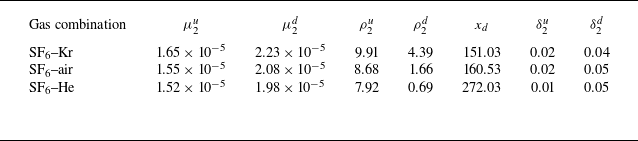
) are summarised in table 2. It is evident that in all scenarios, the values of
 $\delta ^{{u}}_2$
and
 $\delta ^{{d}}_2$
are significantly smaller than the height of the experimental flow field. This indicates that the interface exhibits limited three-dimensional features, suggesting that the boundary layer at the interface has a negligible influence on the perturbation evolution.
Boundary-layer displacement thickness at the twice-shocked interface (
 $\delta _2$
) and relevant parameters:
 $\mu^{{u}}_{2}$
and
 $\mu^{{d}}_{2}$
(
 $\rho ^{{u}}_{2}$
and
 $\rho ^{{d}}_{2}$
) are viscosity coefficients (densities) of post-reshock gases u and d, respectively;
 $x_d$
is the maximum distance between the twice-shocked interface and TS
 $_2$
during the experiment;
 $\delta ^{{u}}_2$
and
 $\delta ^{{d}}_2$
are
 $\delta _2$
upstream and downstream of the interface, respectively. Units of parameters representing viscosity coefficient, density and distance are Pa s, kg m
 $^{-3}$
and mm, respectively.

3. Evolution law of S-RMI under diverse Atwood number conditions
For a once-shocked interface with scaled initial amplitude (
 $|ka_0|$
, where
 $k$
represents the perturbation wavenumber, and
 $a_0$
denotes the initial amplitude which is presumed to be negative) satisfying the small-amplitude criterion (
 $|ka| \ll 1$
), previous research Zhou (Reference Zhou2017a
,Reference Zhou
b
, Reference Zhou2024) suggests that its evolution can be broadly divided into six successive stages: shock-compression stage (perturbation amplitude, denoted as
 $|a_1|$
, decreases under compression), start-up stage (amplitude growth rate, denoted as
 $\dot {a}_{1}$
, increases gradually), linear stage (
 $\dot {a}_{1}$
maintains nearly constant), weakly nonlinear stage (
 $\dot {a}_{1}$
decreases, with bubble and spike structures gradually becoming prominent), strongly nonlinear stage (roll-up structures emerge), and turbulent mixing stage (multiscale vortices appear and intense mixing of substances occurs). Notably, once the interface evolution enters the strongly nonlinear stage, the mixing of substances on two sides of the interface begins. This highlights the importance of suppressing the instability prior to the onset of the strongly nonlinear regime in practical applications. Therefore, the present study focuses on scenarios where the pre-reshock interface has not yet entered the strongly nonlinear regime.
The evolution state of the pre-reshock interface, which is determined by
 $\Delta t$
for given shocks and initial interface, would significantly affect the post-reshock flow evolution (Karkhanis & Ramaprabhu Reference Karkhanis and Ramaprabhu2019; Cao et al. Reference Cao, Chen, Wang, Zhai and Luo2024). Specifically, if reshock occurs before the phase inversion (i.e. a process during which the absolute perturbation amplitude gradually decreases to zero) is completed, the vorticity deposited by IS
 $_2$
has the same sign as that deposited by IS
 $_1$
. Moreover, the vorticity deposition decreases with increasing
 $\Delta t$
, due to the diminished interface amplitude during the phase-inversion process. Conversely, if reshock occurs after the phase inversion is completed, the vorticity deposited by IS
 $_2$
has the opposite sign to that deposited by IS
 $_1$
, and a larger amount of vorticity is deposited for longer
 $\Delta t$
, due to the larger pre-reshock amplitude. Therefore, to better understand the evolution law of S-RMI under diverse
 $A$
conditions, two experimental runs with the same initial perturbation but varying
 $\Delta t$
are conducted for each gas combination (SF
 $_6$
–Kr, SF
 $_6$
–air and SF
 $_6$
–He). The perturbation wavelength
 $\lambda$
and
 $|ka_0|$
are fixed at 40 mm and 0.19, respectively, and the experiments are labelled by the combination of
 $|A_1|$
and
 $\Delta t$
.
3.1. Flow features and interface morphology
Schlieren photographs of experimental cases with various
 $A_1$
and
 $\Delta t$
.

Schlieren images of experiments with different
 $A_1$
and
 $\Delta t$
are presented in figure 4. In all six experiments, the pre-reshock interface remains in the linear or weakly nonlinear regime, meeting the research needs. Case 0.67-566 is selected to exemplify the general interface evolution process. The interface amplitude decreases after the first shock impact, and the phase-inversion process is completed prior to the arrival of IS
 $_2$
(543
 $\unicode{x03BC} \textrm {s}$
). Following the reshock, the interface amplitude decreases gradually (543–1003
 $\unicode{x03BC} \textrm {s}$
). In cases with relatively short
 $\Delta t$
(i.e. cases 0.36-553, 0.67-235 and 0.83-202), the interface has just completed the phase-inversion process when IS
 $_2$
arrives, with amplitude remaining small. After the reshock, the interface amplitude continues to grow. In contrast, for cases with relatively long
 $\Delta t$
(i.e. cases 0.36-1043, 0.67-566 and 0.83-529), the interface amplitude has increased to a considerable level prior to the reshock, and the interface undergoes a second phase-inversion process after the reshock. Additionally, in cases with higher
 $|A_1|$
, the interface evolves at an overall faster rate in both the pre- and post-reshock phases. These observations qualitatively indicate that both
 $A_1$
and
 $\Delta t$
affect the evolution state of the pre-reshock interface, which subsequently influences the post-reshock evolution. In the following, quantitative analyses on the amplitude evolution of the once-shocked and twice-shocked interfaces are performed.
3.2. Once-shocked interface
To predict the complete amplitude evolution of a once-shocked heavy–light interface, Zhai et al. (Reference Zhai, Chen, Xing, Li, Cao, Wang and Luo2025) proposed a combined model (FS model) that comprehensively considers the shock-compression, start-up, linear and weakly nonlinear evolution stages. The construction of the FS model is detailed as follows. To facilitate understanding, the flow features (including wave patterns and interface deformation) at various stages of the once-shocked interface evolution, along with the key physical parameters associated with the FS model, are illustrated in figure 5.
Flow features (including wave patterns and interface deformation) and associated key physical parameters at various stages of the once-shocked interface evolution.

3.2.1. Shock-compression stage
Following the impact of IS
 $_1$
on the initial interface at
 $t=0$
,
 $|a_1|$
decreases continuously until the completion of the shock–interface interaction (Richtmyer Reference Richtmyer1960). The expressions for the duration of the interaction (
 $t_1$
) and the amplitude variation during this stage were proposed by Richtmyer (Reference Richtmyer1960), and can be written as
 \begin{equation} t_1=2\,|a_0|/v_1^{\textit{is}}, \end{equation}
 \begin{equation} a_1(t)=a_0+\Delta u_{1}\,t/2. \end{equation}
These relations, collectively referred to as the R model hereafter, have been extensively validated (Zhou Reference Zhou2024), and were incorporated into the FS model.
3.2.2. Start-up stage
During this stage,
 $\dot {a}_{1}(t)$
rises from zero and gradually reaches an asymptotic value
 $\dot {a}_{1}^{+}$
under the drive of pressure perturbation (Yang, Zhang & Sharp Reference Yang, Zhang and Sharp1994). Lombardini & Pullin (Reference Lombardini and Pullin2009) proposed an analytical model to forecast the characteristic time of the start-up process for a once-shocked light–heavy interface. For a once-shocked heavy–light interface, Yang et al. (Reference Yang, Zhang and Sharp1994) deduced a compressible linear theory to predict the perturbation evolution in the start-up period. However, this theory needs to be solved numerically. Recently, following the approach of Lombardini & Pullin (Reference Lombardini and Pullin2009), Li et al. (Reference Li, Chen, Zhai and Luo2024) deduced an analytical solution for predicting the duration of the start-up process for a once-shocked heavy–light interface, which can be expressed as
 \begin{equation} t_{2}-t_{1}=\dfrac {1}{k}\left (\dfrac {1-A_{1}}{v_{1}^{rw}+\Delta u_{1}}+\dfrac {1+A_{1}}{v_{1}^{\textit{ts}}-\Delta u_{1}}\right ). \end{equation}
Here,
 $t_{2}$
denotes the end moment of the start-up period, while
 $v_{1}^{rw}$
represents the velocity of RW
 $_1$
. In addition, Li et al. (Reference Li, Chen, Zhai and Luo2024) proposed that the amplitude growth in the start-up stage can be described as
 \begin{equation} \dot {a}_{1}(t)=\dfrac {2\dot {a}_{1}^{+}}{(1+A_{1})\coth \big(kL^{\textit{ts}}_1\big)+(1-A_{1})\coth \big(kL^{rw}_1\big)} \quad (t_1\lt t\lt t_2), \end{equation}
where
 \begin{equation} \begin{cases} L^{\textit{ts}}_1= \big(v_{1}^{\textit{ts}}-\Delta u_{1}\big)(t-t_{1}),\\ L^{rw}_1=\big(v_{1}^{rw}+\Delta u_{1}\big)(t-t_{1}), \end{cases} \end{equation}
are the displacements of TS
 $_1$
and RW
 $_1$
, respectively.
3.2.3. Linear stage
When
 $t\gt t_2$
, the amplitude evolution is commonly regarded as entering the linear stage, during which
 $\dot {a}_{1}(t)$
remains nearly constant at
 $\dot {a}_{1}^{+}$
. However, the linear stage is an approximate description of a period where nonlinearity exists but remains limited, and defining the demarcation point between the linear and nonlinear stages is challenging. Therefore, the FS model considers the end of the start-up period as the beginning of both the linear and nonlinear stages. In other words, the linear stage is considered to be of negligible duration in the FS model. The irrotational WN model (WNi model) (Wouchuk & Nishihara Reference Wouchuk and Nishihara1997; Wouchuk Reference Wouchuk2001), validated for scenarios where the shock intensity (defined as
 $1-p_{in}/p_{be}$
, where
 $p_{in}$
and
 $p_{be}$
represent the pressures of fluids in front of and behind the shock, respectively) is lower than 0.5 (Li et al. Reference Li, Chen, Zhai and Luo2024), was adopted to predict
 $\dot {a}_{1}^{+}$
. The WNi model can be written as
 \begin{equation} \dot {a}_1^{+}=k a_{0} \left [\dfrac {1-A_{1}}{2}\left (1+\dfrac {v^{rw}_{1}}{v_{1}^{\textit{is}}}\right )\left (u_{1}-\Delta u_{1}\right ) +\Delta u_{1} \dfrac {1+A_{1}}{2}\left (1-\dfrac {v^{\textit{ts}}_{1}}{v_{1}^{\textit{is}}}\right )\right ], \end{equation}
where
 $u_{1}$
represents the velocity of the fluid behind IS
 $_{1}$
. The system (3.3)–(3.6), collectively referred to as the Li model, was incorporated into the FS model.
3.2.4. Weakly nonlinear stage
As high-order harmonics emerge and become significant,
 $\dot {a}_{1}(t)$
decreases progressively, signifying that the interface evolution has entered the weakly nonlinear stage (Zhou Reference Zhou2024). Zhai et al. (Reference Zhai, Chen, Xing, Li, Cao, Wang and Luo2025) experimentally demonstrated that the DR model (Dimonte & Ramaprabhu Reference Dimonte and Ramaprabhu2010) accurately describes the weakly nonlinear evolution of a once-shocked SF
 $_6$
–air interface, and therefore adopted it to construct the FS model. The DR model can be expressed as
 \begin{equation} \begin{cases} \dot {a}_{1}(t)=\big[\dot {a}^{b}_{1}(t)+\dot {a}^{s}_{1}(t)\big]/2, \\ \dot {a}^{b/s}_{1}(t)=\dot {a}_1^{+}\dfrac {1+k\dot {a}_1^{+} (t-t_2)(1\mp |A_1|)}{1+E^{b/s}k\dot {a}_1^{+} (t-t_2)+(1\mp |A_1|)F^{b/s}k^2 \dot {a}_1^{+2} (t-t_2)^2}, \end{cases} \end{equation}
where superscripts
 $b$
and
 $s$
represent bubble and spike, respectively,
 $E^{b/s}=[4.5\pm |A_1|+(2\mp |A_1|)(1-\Delta u_1/v_1^{\textit{is}})k|a_0|]/4$
and
 $F^{b/s}=1\pm |A_1|$
.
Overall amplitude evolutions of once-shocked heavy–light interfaces with various
 $A_1$
. Symbols denote experimental results; dashed and solid lines represent theoretical predictions by the FS and mFS models, respectively. Error bars represent potential errors in extracting the interface amplitude, with a length equal to half the width of the interface in the experimental schlieren image, and the same hereafter.

The comparison between the present experimental results and corresponding theoretical predictions by the FS model, composed of (3.1)–(3.7), is illustrated in figure 6. It can be observed that the FS model provides reasonable predictions for the entire amplitude evolution process under low and moderate
 $|A_1|$
conditions, as well as for the evolution of the SF
 $_6$
–He interface from the shock-compression to linear stages. However, this model fails to accurately predict the weakly nonlinear evolution of the SF
 $_6$
–He interface. Notably, the R and Li models have been demonstrated to be valid over a wide range of
 $A_1$
conditions (Xing et al. Reference Xing, Chen, Li, Wang, Zhai and Luo2025). Therefore, the failure of the FS model should be attributed to the limitation of the DR model. In our previous work (Xing et al. Reference Xing, Chen, Li, Wang, Zhai and Luo2025), an empirical nonlinear model (mSEA model) was proposed based on existing models and extensive experimental results (Chen et al. Reference Chen, Xing, Wang, Zhai and Luo2023; Xing et al. Reference Xing, Chen, Li, Wang, Zhai and Luo2025), which can be described as
 \begin{equation} \begin{cases} \dot {a}_{1}(t)=\big[\dot {a}^{b}_{1}(t)+\dot {a}^{s}_{1}(t)\big]/2, \\ \dot {a}^{b/s}_{1}(t)=\dot {a}_1^{+}\dfrac {1+k\dot {a}_1^{+} (t-t_2)}{1+(2\mp |A_1|)(1.07\pm |A_1|)k\dot {a}_1^{+} (t-t_2)+\dfrac {1\pm |A_{1}|}{1+|A_{1}|}\dfrac {1}{2\pi C_1}k^2 \dot {a}_1^{+2} (t-t_2)^2}, \end{cases} \end{equation}
where
 $C_1$
is given by
 $1/3\pi$
for cases with
 $|A_{1}|\geqslant 0.5$
, and
 $1/2\pi$
for cases where
 $|A_{1}|\rightarrow 0$
. The mSEA model has been shown to effectively describe the weakly nonlinear evolution across the ranges of
 $A_1$
from
 $-0.95$
to
 $-0.35$
, and from 0.30 to 0.86. Therefore, we can obtain a modified FS model (mFS model) by substituting the DR model with the mSEA model. The overall amplitude evolution predicted using the mFS model is presented in figure 6. The close agreement between the mFS model predictions and experimental results suggests that the mFS model is capable of reliably predicting the complete amplitude evolution of once-shocked heavy–light interfaces with various
 $A_1$
.
3.3. Twice-shocked interface
Given the complex characteristics of the pre- and post-reshock flow fields, two simplifying assumptions are made in developing the models for the twice-shocked interface evolution. First, the influence of the rippled RW
 $_1$
on IS
 $_2$
is negligible, i.e. IS
 $_2$
can be treated as a planar shock. Second, the non-uniformities in the flow field behind TS
 $_1$
have a negligible influence on TS
 $_2$
, i.e. the flow field ahead of TS
 $_2$
can be approximated as uniform. An evaluation of these two assumptions is provided in Appendix C. Moreover, to aid comprehension of the model construction, the flow features and associated key physical parameters at diverse stages following the reshock are sketched in figure 7. Notably, multiple scenarios may arise depending on the pre-reshock interface configuration and the subsequent post-reshock evolution. The flow depicted in figure 7 represents a typical case in which the reshock occurs after the phase inversion of the once-shocked interface, and the twice-shocked interface subsequently undergoes a second phase inversion.
Flow features and associated key physical parameters at diverse stages following reshock. The flow depicted represents a typical case in which the reshock occurs after the phase inversion of the once-shocked interface, and the twice-shocked interface subsequently undergoes a second phase inversion.

3.3.1. Linear amplitude growth
To describe the linear evolution following reshock, Mikaelian (Reference Mikaelian1985) proposed a linear superposition principle, which assumes that the post-reshock linear amplitude growth rate (
 $\dot {a}_{2}^{+}$
) is equal to the linear superposition of the pre-reshock amplitude growth rate (
 $\dot {a}_{2}^{-}$
) and the additional growth rate induced by reshock (
 $\Delta \dot {a}$
). This principle has since served as a theoretical basis for numerous investigations. Specifically, the Mik-L model proposed by Mikaelian (Reference Mikaelian1985) assumes that
 $\dot {a}_{2}^{+}$
equals the sum of
 $\dot {a}_{2}^{-}$
and
 $\Delta \dot {a}$
calculated using the impulsive model. As a result, the Mik-L model is applicable only for scenarios with a light–heavy interface, and is expected to fail when reshock occurs at the nonlinear evolution stage of the once-shocked interface. Building upon the linear superposition principle, Charakhch’yan (Reference Charakhch’yan2000, Reference Charakhch’yan2001) proposed the Cha-L model for predicting
 $\dot {a}_{2}^{+}$
. However, the Cha-L model does not include a relation/model to predict the amplitude evolution of the once-shocked interface, and instead relies on
 $\dot {a}_{2}^{-}$
extracted from numerical simulations or experiments. Thus its application is significantly constrained. Additionally, the Cha-L model is expected to be applicable only when reshock occurs at strongly nonlinear stages, as it assumes that
 $\Delta \dot {a}$
is independent of the pre-reshock perturbation characteristics. To address the limitations of the previous models, Zhai et al. (Reference Zhai, Chen, Xing, Li, Cao, Wang and Luo2025) proposed a new model (LS model) to predict
 $\dot {a}_{2}^{+}$
of an SF
 $_6$
–air interface subjected to reshock occurring at any stage prior to the onset of strong nonlinearity. The LS model can be expressed as
 \begin{equation} \dot {a}_{2,ls}^{+}=\dot {a}_{2,fs}^{-}+\Delta \dot {a}_{wni}, \end{equation}
where
 \begin{align} \Delta \dot {a}_{wni}&=k a_{2,fs}^{-} \left [\dfrac {1-A_{2}}{2}\left (1+\dfrac {v^{rw}_{2}+\Delta u_{1}}{v_{2}^{\textit{is}}-\Delta u_{1}}\right )(u_{2}-\Delta u_{1}-\Delta u_{2}) \right. \nonumber \\ & \quad + \left. \Delta u_{2} \dfrac {1+A_{2}}{2}\left (1-\dfrac {v^{\textit{ts}}_{2}-\Delta u_{1}}{v_{2}^{\textit{is}}-\Delta u_1}\right )\right ] \end{align}
represents
 $\Delta \dot {a}$
predicted by the WNi model;
 $\dot {a}_{2,fs}^{-}$
and
 $a_{2,fs}^{-}$
correspond to
 $\dot {a}_{2}^{-}$
and the pre-reshock amplitude (
 $a_{2}^{-}$
) predicted by the FS model, respectively;
 $v_2^{rw}$
and
 $u_2$
denote the velocities of RW
 $_2$
and the fluid behind IS
 $_{2}$
, respectively;
 $A_2$
represents the post-reshock Atwood number.
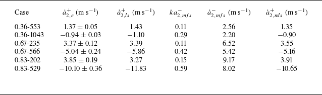
Experimental and theoretical results related to the post-reshock linear amplitude evolution:
 $\dot {a}_{2,e}^{+}$
,
 $\dot {a}^{+}_{2,ls}$
and
 $\dot {a}^{+}_{2,mls}$
are post-reshock linear amplitude growth rates obtained from experiments and predicted by the LS and mLS models, respectively;
 $ka^{-}_{2,mfs}$
and
 $\dot {a}^{-}_{2,mfs}$
are pre-reshock dimensionless amplitude and amplitude growth rate predicted by the mFS model, respectively.

Values of
 $\dot {a}_{2}^{+}$
extracted from experiments (
 $\dot {a}_{2,e}^{+}$
) and predicted by the LS model are presented in table 3. It can be observed that the LS model reasonably forecasts
 $\dot {a}_{2,e}^{+}$
for cases 0.36-553, 0.36-1043 and 0.67-235, whereas it performs poorly in predicting
 $\dot {a}_{2,e}^{+}$
for cases 0.67-566, 0.83-202 and 0.83-529. The failure of the LS model for case 0.67-566 should be attributed to the fact that
 $ka_2^{-}$
no longer satisfies the small-amplitude criterion, which is a fundamental assumption for the validity of the WNi model. Extensive research (Rikanati et al. Reference Rikanati, Oron, Sadot and Shvarts2003; Dimonte & Ramaprabhu Reference Dimonte and Ramaprabhu2010; Probyn et al. Reference Probyn, Williams, Thornber, Drikakis and Youngs2021; Wang et al. Reference Wang, Wang, Zhai and Luo2023a
,Reference Wang, Wang, Zhai and Luo
b
) has demonstrated that the high initial amplitude leads to the practical linear amplitude growth rate being lower than the predictions from models deduced based on the small-amplitude assumption – a phenomenon generally referred to as the high-amplitude effect. Several reduction factors have been proposed to describe this effect (Rikanati et al. Reference Rikanati, Oron, Sadot and Shvarts2003; Dimonte & Ramaprabhu Reference Dimonte and Ramaprabhu2010; Probyn et al. Reference Probyn, Williams, Thornber, Drikakis and Youngs2021; Wang et al. Reference Wang, Wang, Zhai and Luo2023b
). Among them, the one proposed by Dimonte & Ramaprabhu (Reference Dimonte and Ramaprabhu2010) (
 $R_{\textit{dr}}$
) has been demonstrated to effectively describe the high-amplitude effect on the evolution of a once-shocked heavy–light interface (Wang et al. Reference Wang, Wang, Zhai and Luo2023a
). In contrast, for case 0.83-202, where
 $ka_2^{-}$
still satisfies the small-amplitude criterion, the failure of the LS model should be attributed to the fact that the FS model loses accuracy under high
 $|A_1|$
conditions, as demonstrated in § 3.2. For case 0.83-529, the failure of the LS model results from the combined influence of the high-amplitude effect and the limitation of the FS model.
Here, we propose a modified model (mLS model) to predict
 $\dot {a}_{2}^{+}$
by combining the linear superposition principle, WNi model, mFS model and
 $R_{\textit{dr}}$
, expressed as
 \begin{equation} \dot {a}_{2,mls}^{+}=\dot {a}_{2,mfs}^{-}+\Delta \dot {a}_{wni}\times R_{\textit{dr}}=\dot {a}_{2,mfs}^{-}+\dfrac {\Delta \dot {a}_{wni}} {1+\big (|ka_{2,mfs}^{-}|/3\big )^{4/3}}, \end{equation}
where
 \begin{align} \Delta \dot {a}_{wni}&=k a_{2,mfs}^{-} \left [\dfrac {1-A_{2}}{2}\left (1+\dfrac {v^{rw}_{2}+\Delta u_{1}}{v_{2}^{\textit{is}}-\Delta u_{1}}\right )(u_{2}-\Delta u_{1}-\Delta u_{2}) \right. \nonumber \\ & \quad + \left.\Delta u_{2} \dfrac {1+A_{2}}{2}\left (1-\dfrac {v^{\textit{ts}}_{2}-\Delta u_{1}}{v_{2}^{\textit{is}}-\Delta u_1}\right )\right ], \end{align}
and
 $\dot {a}_{2,mfs}^{-}$
and
 $a_{2,mfs}^{-}$
correspond to
 $\dot {a}_{2}^{-}$
and
 $a_{2}^{-}$
predicted by the mFS model, respectively. As presented in table 3, the mLS model is capable of accurately predicting the linear amplitude evolution of a twice-shocked heavy–light interface under diverse
 $A_1$
and
 $\Delta t$
conditions.
3.3.2. Complete amplitude evolution
Understanding the post-reshock linear amplitude evolution is essential. However, achieving a full-process prediction of the twice-shocked interface evolution remains a more desirable objective. Existing models, including the Mik-L, Cha-L, LS and mLS models, are limited to predicting only
 $\dot {a}_{2}^{+}$
, without capturing the full temporal evolution. We therefore aim to develop a theoretical model that accurately describes the complete post-reshock evolution. Analogous to the development of a once-shocked interface, the evolution of a twice-shocked interface can be broadly divided into the shock-compression stage, start-up stage, linear stage, weakly nonlinear stage, strongly nonlinear stage and turbulent mixing stage. In this study, we focus exclusively on the evolution preceding the strongly nonlinear stage. The time-varying amplitude growth rate and amplitude of the twice-shocked interface are represented by
 $\dot {a}_{2}(t)$
and
 $a_{2}(t)$
, respectively. The details of the model construction are provided below.
Shock-compression stage: The velocity of IS
 $_2$
relative to the once-shocked interface is typically much greater than
 $\dot {a}_{2}^{-}$
. Consequently, as IS
 $_2$
propagates across the interface, the interface can be approximated as moving with velocity
 $\Delta u_1$
without undergoing any self-evolution. Accordingly, the duration of the shock-compression stage (
 $t_3-\Delta t$
) and
 $a_{2}(t)$
in this stage can also be predicted using the R model:
 \begin{equation} t_3-\Delta t=2a_{2,mfs}^{-}/\big(v_2^{\textit{is}}-\Delta u_1\big), \end{equation}
 \begin{equation} a_2(t)=a_{2,mfs}^{-}-\Delta u_2 \big(t-\Delta t\big)/2. \end{equation}
Start-up stage: The twice-shocked interface enters the start-up evolution stage (
 $t_3\lt t\lt t_4$
) once IS
 $_2$
has completely traversed the interface. Following the idea of linear superposition, the start-up evolution of the twice-shocked interface is considered as a process wherein
 $\dot {a}_{2}(t)$
varies from
 $\dot {a}_{2}^{-}$
to
 $\dot {a}_{2}^{+}$
under the drive of pressure perturbations introduced by the perturbed TS
 $_2$
and RW
 $_2$
. Accordingly, the duration of the start-up process of the twice-shocked interface (
 $t_4 - t_3$
) and
 $\dot {a}_{2}(t)$
in this stage can be described by the reformulated Li model:
 \begin{equation} t_{4}-t_{3}=\dfrac {1}{k}\left (\dfrac {1-A_{2}}{v_{2}^{rw}+\Delta u_{1}+\Delta u_{2}}+\dfrac {1+A_{2}}{v_{2}^{\textit{ts}}-\Delta u_{1}-\Delta u_{2}}\right ), \end{equation}
 \begin{equation} \dot {a}_{2}(t)=\dot {a}_{2}^{-}+\dfrac {2\,\Delta \dot {a}}{(1+A_{2})\coth \big(kL^{\textit{ts}}_2\big)+(1-A_{2})\coth \big(kL^{rw}_2\big)}, \end{equation}
where
 $L^{\textit{ts}}_2$
and
 $L^{rw}_2$
denote the displacements of TS
 $_2$
and RW
 $_2$
, respectively, which can be expressed as
 \begin{equation} \begin{cases} L^{\textit{ts}}_2= \big(v_{2}^{\textit{ts}}-\Delta u_{1}-\Delta u_{2}\big)(t-t_{3}),\\ L^{rw}_2=\big(v_{2}^{rw}+\Delta u_{1}+\Delta u_{2}\big)(t-t_{3}). \end{cases} \end{equation}
Linear stage: Similarly, the linear evolution stage of the twice-shocked interface is considered to have a negligible duration, during which
 $\dot {a}_{2}$
remains constant at
 $\dot {a}_{2}^{+}$
. The mLS model, which has been validated earlier, is employed to predict
 $\dot {a}_{2}^{+}$
. Specifically,
 $\dot {a}_{2}^{-}$
and
 $\Delta \dot {a}$
in (3.16) are given by
 $\dot {a}_{2,mfs}^{-}$
and
 $\Delta \dot {a}_{wni} \times R_{\textit{dr}}$
, respectively.
Weakly nonlinear stage: Currently, there is still a lack of nonlinear models specifically proposed for the twice-shocked interface. Our previous study (Wang et al. Reference Wang, Cao, Chen, Zhai and Luo2022) demonstrated that for a light–heavy interface configuration, the evolution of a twice-shocked interface can be reasonably predicted by models developed for once-shocked interfaces, provided that the reshock occurs prior to the strongly nonlinear stage. This suggests that it is potentially feasible to treat a twice-shocked heavy–light interface as a once-shocked one with equivalent post-shock amplitude and linear growth rate. Based on this idea, the weakly nonlinear evolution of twice-shocked heavy–light interfaces with varying
 $A$
is also described using the mSEA model reformulated as
 \begin{equation} \begin{cases} \dot {a}_{2}(t)=\big[\dot {a}^{b}_{2}(t)+\dot {a}^{s}_{2}(t)\big]/2, \\ \dot {a}^{b/s}_{2}(t)=\dot {a}_{2,mls}^{+} \dfrac {1+k\dot {a}_{2,mls}^{+} (t-t_4)}{1+(2\mp |A_2|)(1.07\pm |A_2|)k\dot {a}_{2,mls}^{+} (t-t_4)+\dfrac {1\pm |A_{2}|}{1+|A_{2}|}\dfrac {1}{2\pi C_2}k^2 \dot {a}_{2,mls}^{+2} (t-t_4)^2}, \end{cases} \end{equation}
where
 $C_2$
is given by
 $1/3\pi$
for cases with
 $|A_{2}|\geqslant 0.5$
, and
 $1/2\pi$
for cases with
 $|A_{2}|\rightarrow 0$
. For clarity, the combination of (3.11)–(3.18) is hereafter referred to as the DS model. As illustrated in figure 8, the DS model offers accurate predictions for the amplitude evolution from the instant IS
 $_2$
hits the once-shocked interface to the weakly nonlinear evolution stage of the twice-shocked interface under diverse
 $A$
and
 $\Delta t$
conditions.
In conclusion, two models, namely the mFS and DS models, have been developed based on existing theoretical models and physically justified assumptions. Experimental validation confirms that, when combined, they can reliably predict the complete perturbation evolution of S-RMI across a wide range of
 $A$
. In the following, we will employ these models to achieve the controllable suppression of RMI via a same-side reshock under low, moderate and high
 $|A|$
conditions.
Amplitude evolution of twice-shocked interface under diverse
 $A$
and
 $\Delta t$
conditions. Symbols and solid lines denote experimental results and theoretical predictions by the DS model, respectively.

Schematics of seven possibilities for S-RMI at an initial heavy–light interface without Atwood-number reversal (
 $A_0\lt 0$
and
 $A_1\lt 0$
).

Parameter conditions corresponding to each perturbation evolution possibility for scenarios with various
 $A$
. Open circles denote the experimental cases that have been discussed in § 3, whereas solid circles represent the supplementary experimental runs.

4. Experimental realisation of instability suppression
Building upon the possibility analysis of Mikaelian (Reference Mikaelian1985), Zhai et al. (Reference Zhai, Chen, Xing, Li, Cao, Wang and Luo2025) systematically discussed the possible amplitude evolution patterns. However, both analyses are based on the assumption of incompressibility. In certain compressible scenarios, such as RMI at a light–heavy interface where the light gas exhibits strong compressibility, the heavy gas is weakly compressible, and the initial density contrast is moderate, an Atwood-number-reversal phenomenon (i.e.
 $A_1$
possesses an opposite sign to
 $A_0$
) may occur (Mikaelian Reference Mikaelian1994). Under such compressible conditions, the previous incompressible analyses become less rigorous. A detailed discussion of the perturbation evolution possibilities in a compressible two-co-propagating-shock system is provided in Appendix B.
In the present experiments, since the heavy gas (SF
 $_6$
) is characterised by a relatively high compressibility, and the light gas (Kr, air and He) by a relatively low compressibility,
 $A_1$
retains the same sign as
 $A_0$
. In other words, the present experiments correspond to compressible S-RMI scenarios without Atwood-number reversal. According to Appendix B, the analyses by Mikaelian (Reference Mikaelian1985) and Zhai et al. (Reference Zhai, Chen, Xing, Li, Cao, Wang and Luo2025) for incompressible S-RMI remain valid under the present experimental conditions: seven distinct evolution patterns arise, depending on the relative signs and magnitudes of
 $\dot {a}_{2}^{-}$
and
 $\dot {a}_{2}^{+}$
, as depicted in figure 9. Among them, the suppression of RMI growth (
 $|\dot {a}_{2}^{+}|\lt \dot {a}_{2}^{-}$
) occurs in possibilities III-HL, IV-HL and V-HL. In particular, in possibility IV-HL, where
 $\dot {a}_{2}^{+}=0$
, the freeze-out phenomenon occurs.
Schlieren photographs of experimental cases in which the amplitude growth is theoretically predicted to be suppressed by the same-side reshock.

Based on the mFS and DS models, and the general 1-D experimental parameters presented in table 1, theoretical lines corresponding to possibilities II-HL, IV-HL and VI-HL in the
 $(\lambda,\Delta t)$
plane are calculated. The results for cases with
 $A_1$
values
 $-0.36$
,
 $-0.67$
and
 $-0.83$
are depicted in figures 10(a–c), respectively. These lines, referred to as the acceleration line, freeze-out line and reversal line, respectively, partition the plane into four regions, corresponding to possibilities I-HL, III-HL, V-HL and VII-HL. Figure 10 indicates that by keeping the gas combination, initial perturbation and shock intensities constant, the twice-shocked interface evolution can be manipulated by varying
 $\Delta t$
. The six experimental cases with different
 $A$
and
 $\Delta t$
, discussed in § 3, are plotted as open circles in figure 10. For the scenario with low
 $|A|$
, cases 0.36-553 and 0.36-1043 correspond to possibilities III-HL and V-HL, respectively. For the scenario with moderate (high)
 $|A|$
, case 0.67-235 (case 0.83-202) corresponds to possibility III-HL. To realise all three possibilities of instability suppression in each
 $A$
scenario, five additional experimental runs corresponding to possibilities without existing experiments are conducted: IV-HL for the low
 $|A|$
scenario, and IV-HL and V-HL for moderate and high
 $|A|$
scenarios. These runs are represented by solid circles in figure 10.
Figure 11 presents the schlieren images for all nine experimental cases in which the amplitude growth is theoretically predicted to be suppressed by the same-side reshock. In all cases, the interface maintains a quasi-single-mode profile before reshock, indicating that the reshock occurs prior to the strongly nonlinear stage. The complete interface amplitude evolution for these nine cases throughout the effective experimental duration is presented in figure 12, along with the predictions from the mFS and DS models. It is evident that the post-reshock amplitude evolution rate is significantly lower than the pre-reshock one, and all theoretical predictions are in excellent agreement with the experimental results, indicating that all three possibilities for suppressing the RMI growth are achieved under low, moderate and high
 $|A|$
conditions. Overall, the suppression and freeze-out of the RMI growth via a same-side reshock are achievable and predictable under diverse
 $A$
conditions.
Complete interface amplitude evolution for nine experimental cases in which the amplitude growth is theoretically predicted to be suppressed by the same-side reshock. Solid lines represent the theoretical predictions from the mFS and DS models.

5. Conclusions and perspective
This study explores the evolution law and suppression strategy of the Richtmyer–Meshkov instability (RMI) induced by two co-propagating shock waves (S-RMI) across a broad range of Atwood numbers, integrating theoretical and experimental approaches. Experimentally, two co-propagating shocks with controllable time intervals (
 $\Delta t$
) and intensities are generated using a dedicated shock-tube facility (Wang et al. Reference Wang, Cao, Chen, Zhai and Luo2022), while well-defined initial interfaces with varying Atwood numbers are produced via an improved soap-film technique. Previously developed models (Zhai et al. Reference Zhai, Chen, Xing, Li, Cao, Wang and Luo2025) describing the complete evolution of a once-shocked interface and the linear growth of a twice-shocked interface are evaluated under diverse post-first-shock Atwood numbers (
 $-0.36$
,
 $-0.68$
and
 $-0.83$
), and further refined based on detailed analyses of their limitations. Furthermore, an analytical model for describing the complete evolution of a twice-shocked interface (DS model) is developed by comprehensively considering the shock-compression, start-up, linear and weakly nonlinear evolution processes. Shock-tube experiments with various Atwood numbers and
 $\Delta t$
values demonstrate that the combination of the refined models and DS model enables, for the first time, an accurate prediction of the complete evolution of S-RMI. Based on these models and the general one-dimensional flow information, parameter conditions for manipulating the RMI growth are identified. Nine validation experiments with diverse combinations of Atwood numbers and
 $\Delta t$
confirm that the suppression and freeze-out of the RMI growth via a same-side second impact are feasible and predictable across a wide range of Atwood numbers.
This study may offer some insights into the suppression of hydrodynamic instabilities in inertial confinement fusion (ICF) through a same-side reshock. Specifically, by optimising material densities and shock timings within the framework of global implosion dynamics, the early-time perturbation growth induced by RMI could potentially be suppressed through reshock, thereby mitigating the development of the Rayleigh–Taylor (RT) instability (Rayleigh Reference Rayleigh1883; Taylor Reference Taylor1950) in the subsequent deceleration phase. However, we acknowledge that our consideration of a single-mode gaseous interface in planar geometry represents a considerable simplification of the actual ICF scenario. In ICF, the hydrodynamic instabilities arise at multi-material interfaces exhibiting multi-mode perturbations and are driven by co-propagating convergent shock waves. Although the present models have been validated by 11 experiments spanning a range of Atwood numbers and
 $\Delta t$
values, they are not expected to accurately describe more complex flows owing to the presence of additional physical mechanisms. To explore the instability suppression strategies under conditions that more closely resemble those in actual ICF scenarios, we propose the following three future research directions, within which the current models will be further evaluated and refined to address increased physical complexity.
First, consider S-RMI in convergent geometry. In ICF, a convergent geometry implosion scheme is adopted to achieve maximum energy density for a given driver energy. Compared with RMI in planar geometry, RMI in convergent geometry involves additional physical mechanisms. Bell (Reference Bell1951) and Plesset (Reference Plesset1954) analysed the early-time interface instability in convergent geometry, and demonstrated that the radial movement of the interface affects perturbation growth, a phenomenon now referred to as the Bell–Plesset (BP) effect. Additionally, unlike in planar geometry where the interface typically maintains a constant velocity, the interface in convergent geometry generally experiences acceleration or deceleration, thereby giving rise to the RT effect (Lombardini, Pullin & Meiron Reference Lombardini, Pullin and Meiron2014; Ding et al. Reference Ding, Si, Yang, Lu, Zhai and Luo2017b ; Samulski et al. Reference Samulski, Srinivasan, Manuel, Masti, Sauppe and Kline2022). In S-RMI within a convergent geometry, the BP effect, RT effect and same-side reshock are intrinsically coupled, thereby significantly increasing the physical complexity. A novel facility capable of generating two co-propagating convergent shock waves is currently under development. This platform will enable detailed investigations into the evolution mechanisms and potential manipulation strategies for S-RMI in convergent geometry.
Second, consider S-RMI at multi-mode interfaces. In ICF, multi-mode perturbations inevitably arise at the interfaces separating different layers due to the manufacturing defects and material inhomogeneities. Furthermore, critical engineering features, such as the fill tube and the supporting membrane, serve as additional sources of the multi-mode perturbations at the target interfaces (Zhou et al. Reference Zhou, Sadler and Hurricane2025). Therefore, understanding and further suppressing the instability on multi-mode interfaces are necessary and of significant scientific importance. In future work, we will explore the evolution mechanisms and manipulation strategies of S-RMI at multi-mode interfaces, with detailed consideration of the modal coupling and competition.
Third, consider S-RMI at multi-material interfaces. The present study focuses solely on the evolution of S-RMI at gas–gas interfaces. However, ICF targets generally involve multi-material interfaces, such as gas–solid and solid–solid ones. The presence of non-gaseous materials introduces additional physical mechanisms affecting RMI evolution. For example, at gas–hydrogel interfaces, the viscosity and elasticity of the hydrogel can influence RMI evolution, which manifest through viscous dissipation and elastic energy storage, respectively. Future work will investigate the mechanisms and manipulation of S-RMI when non-gaseous materials are present on one or both sides of the interface.
Acknowledgements
The authors sincerely appreciate the reviewers for their valuable suggestions.
Funding
This work was supported by the National Natural Science Foundation of China (nos 12388101, 12472228, 12372281 and 12027801), the Young Elite Scientists Sponsorship Programme by CAST (no. 2023QNRC001), and the Strategic Priority Research Programme of the Chinese Academy of Science (XDB1100120).
Declaration of interests
The authors report no conflict of interest.
Appendix A. Comparison between validation experiments
To evaluate the reliability and repeatability of the experiments, three experimental runs are conducted for each gas combination, following identical procedures. Notably, among three runs with the same gas combination, the first two have similar
 $\Delta t$
, while the third has a relatively longer
 $\Delta t$
, to verify whether the variation in
 $\Delta t$
would affect the general 1-D flow parameters.
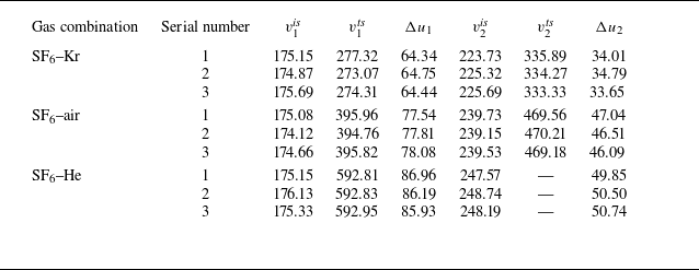
Key parameters of nine validation experiments for evaluating the reliability of the experimental methods:
 $v_1^{\textit{is}}$
and
 $v_1^{\textit{ts}}$
(
 $v_2^{\textit{is}}$
and
 $v_2^{\textit{ts}}$
) are velocities of IS
 $_1$
and TS
 $_1$
(IS
 $_2$
and TS
 $_2$
), respectively;
 $\Delta u_1$
and
 $\Delta u_2$
are jump velocities of the interface induced by IS
 $_1$
and IS
 $_2$
, respectively. Unit of all parameters representing velocity is m s
 $^{-1}$
.

Trajectories of shocks and interface extracted from nine validation experiments. Diverse symbols (circle, square and triangle) represent different experimental runs with the same gas combination: (a) SF
 $_6$
–Kr, (b) SF
 $_6$
–air, (c) SF
 $_6$
–He.

The trajectories and velocities of shock waves and interface, extracted from different experimental runs, are presented in figure 13 and table 4, respectively. These results demonstrate that the 1-D flow parameters are highly consistent across different runs with the same gas combination, confirming the reliability of the experimental approach.
Appendix B. Possible evolution patterns in a compressible two-co-propagating-shock system
In the pioneering work by Mikaelian (Reference Mikaelian1994) on the influence of compressibility on RMI, it was proposed that under certain conditions, such as when the shock intensity is high and the light (heavy) fluid is strongly (weakly) compressible, the Atwood-number reversal, a phenomenon that
 $A_0$
and
 $A_1$
have opposite signs (i.e.
 $A_0 \gt 0$
but
 $A_1 \lt 0$
, or
 $A_0 \lt 0$
but
 $A_1 \gt 0$
), may occur. Although this phenomenon is challenging to realise experimentally due to the physical constraints of available gases, it nonetheless provides additional possibilities for manipulating RMI via a same-side reshock. In the following, analysis is performed to clarify the possible amplitude evolution patterns in a compressible two-co-propagating-shock system, considering scenarios with and without Atwood-number reversal, as well as special cases with
 $A_0 \neq 0$
but
 $A_1 = 0$
. To facilitate analysis, following the conventions of previous studies (Mikaelian Reference Mikaelian1985; Zhai et al. Reference Zhai, Chen, Xing, Li, Cao, Wang and Luo2025), we assume that
 $a_0$
is positive for an initial light–heavy interface, and negative for an initial heavy–light one.
B.1 Initial light–heavy interface
 $(A_0\gt 0)$

An initial light–heavy interface subjected to a shock wave would continue to evolve in the same phase, i.e. no phase inversion would occur. Based on the
 $A_1$
value, there are three distinct scenarios:
 $A_1\gt 0$
,
 $A_1=0$
and
 $A_1\lt 0$
, which are analysed separately below.
B.1.1 Case
$A_0\gt 0$
and
$A_1\gt 0$


For this scenario, the relative orientations of the shock-induced pressure gradient and the interfacial density gradient in the first impact and reshock are identical, such that the vorticity generated by the reshock possesses the same sign as that produced by the first shock. Therefore, for an initial light–heavy interface without Atwood-number reversal, a same-side reshock can only promote the instability (possibility I-LH), consistent with the analysis by Mikaelian (Reference Mikaelian1985) and Zhai et al. (Reference Zhai, Chen, Xing, Li, Cao, Wang and Luo2025) for incompressible S-RMI.
B.1.2 Case
$A_0\gt 0$
and
$A_1=0$


If the light and heavy gases are highly and weakly compressible, respectively, and the initial density contrast is moderate, then
 $A_1$
can approach zero or even become negative, as proposed by Mikaelian (Reference Mikaelian1994). For the scenario with
 $A_1=0$
, since there is no density gradient on the once-shocked interface, the reshock cannot deposit additional vorticity and is therefore expected to exert no influence on the instability (possibility II-LH).
B.1.3 Case
$A_0\gt 0$
and
$A_1\lt 0$


In this case, due to the differing relative orientations of the pressure and density gradients in the first impact and reshock, the vorticity deposited by reshock carries an opposite sign to that induced by the first shock. In other words,
 $\Delta \dot {a}$
is of opposite sign to
 $\dot {a}_{2}^{-}$
. Depending on the relative signs and magnitudes of
 $\dot {a}_{2}^{-}$
and
 $\dot {a}_{2}^{+}$
(
 $= \dot {a}_{2}^{-} + \Delta \dot {a}$
), five distinct evolution scenarios arise, as illustrated in figure 14 and described sequentially below.
Schematics of five possibilities for S-RMI at an initial light–heavy interface with Atwood-number reversal (
 $A_0\gt 0$
and
 $A_1\lt 0$
).

Possibility III-LH:
 $|\Delta \dot {a}| \lt \dot {a}_{2}^{-}$
and
 $0 \lt \dot {a}_{2}^{+} \lt \dot {a}_{2}^{-}$
, i.e. the reshock weakens the instability triggered by the first shock while preserving the original growth trend.
Possibility IV-LH:
 $|\Delta \dot {a}| = \dot {a}_{2}^{-}$
and
 $\dot {a}_{2}^{+} = 0$
, i.e. the reshock eliminates the instability at the once-shocked interface, resulting in a freeze-out phenomenon.
Possibility V-LH:
 $\dot {a}_{2}^{-} \lt |\Delta \dot {a}| \lt 2 \dot {a}_{2}^{-}$
and
 $-\dot {a}_{2}^{-} \lt \dot {a}_{2}^{+} \lt 0$
, i.e. the reshock not only attenuates the instability but also reverses the trend of perturbation growth.
Possibility VI-LH:
 $|\Delta \dot {a}| = 2 \dot {a}_{2}^{-}$
and
 $\dot {a}_{2}^{+} = -\dot {a}_{2}^{-}$
, i.e. the reshock reverses the evolution trend of RMI growth without changing its rate.
Possibility VII-LH:
 $|\Delta \dot {a}| \gt 2 \dot {a}_{2}^{-}$
and
 $\dot {a}_{2}^{+} \lt -\dot {a}_{2}^{-}$
, i.e. the reshock both reverses the perturbation growth trend and enhances the instability.
B.2 Initial heavy–light interface (
$A_0\lt 0$
)

For an initial heavy–light interface subjected to a shock wave, it would undergo a phase-inversion process, i.e. the amplitude first decreases over time, becoming zero, then grows in the opposite phase. Similarly, in terms of
 $A_1$
, there are three distinct scenarios:
 $A_1\lt 0$
,
 $A_1=0$
and
 $A_1\gt 0$
, each of which is analysed separately below.
B.2.1 Case
$A_0\lt 0$
and
$A_1\lt 0$


Since
 $A_0$
and
 $A_1$
share the same sign, if reshock occurs during the phase-inversion process, then the relative orientations of the pressure and density gradients in the first impact and reshock are identical. As a result, the reshock would enhance the instability (possibility I-HL), as illustrated in figure 9(a). In contrast, if the reshock occurs exactly at the moment the phase inversion is completed, then the interface is planar, leading to collinearity between the pressure and density gradients. In this case, the reshock would not affect the instability (possibility II-HL), as illustrated in figure 9(b). If the reshock occurs after phase inversion, then the relative orientations of the pressure and density gradients in the first impact and reshock are opposite. For this scenario, there are five distinct possibilities (possibilities III-HL to VII-HL), depending on the relative signs and magnitudes of
 $\dot {a}_{2}^{-}$
and
 $\dot {a}_{2}^{+}$
, as illustrated in figures 9(c–g). Details on these possibilities can be found in a previous work (Zhai et al. Reference Zhai, Chen, Xing, Li, Cao, Wang and Luo2025) and thus are not repeated here.
B.2.2 Case
$A_0\lt 0$
and
$A_1=0$


For an initial heavy–light interface, if the heavy and light gases are weakly and strongly compressible, respectively, and the density contrast is moderate, then the first impact may yield either
 $A_1 = 0$
or
 $A_1 \gt 0$
. For the scenario with
 $A_1 = 0$
, since the density gradient across the once-shocked interface vanishes, the reshock would not deposit additional vorticity regardless of its timing. Accordingly, the reshock is expected to have no influence on the instability (possibility VIII-HL).
B.2.3 Case
$A_0\lt 0$
and
$A_1\gt 0$


Since
 $A_0$
and
 $A_1$
have opposite signs, if reshock occurs during the phase-inversion process, then the relative orientations of the pressure and density gradients in the first impact and reshock are opposite. In other words,
 $\Delta \dot {a}$
has sign opposite to that of
 $\dot {a}_{2}^{-}$
. Depending on the relative signs and magnitudes of
 $\dot {a}_{2}^{-}$
and
 $\dot {a}_{2}^{+}$
, there are five possible evolution patterns, as illustrated in figures 15(a–e) and described sequentially below.
Schematics of seven possibilities for S-RMI at an initial heavy–light interface with Atwood-number reversal (
 $A_0\lt 0$
and
 $A_1\gt 0$
).

Possibility VIIII-HL:
 $|\Delta \dot {a}| \gt 2\dot {a}_{2}^{-}$
and
 $-\dot {a}_{2}^{+} \gt \dot {a}_{2}^{-}$
, i.e. the reshock promotes the instability induced by the first shock and simultaneously alters its evolution trend.
Possibility
 $\Delta$
-HL:
 $|\Delta \dot {a}| = 2\dot {a}_{2}^{-}$
and
 $-\dot {a}_{2}^{+} = \dot {a}_{2}^{-}$
, i.e. the reshock reverses the evolution trend of RMI growth without changing its rate.
Possibility
 $\Delta$
I-HL:
 $\dot {a}_{2}^{-} \lt |\Delta \dot {a}| \lt 2\dot {a}_{2}^{-}$
and
 $0 \lt -\dot {a}_{2}^{+} \lt \dot {a}_{2}^{-}$
, i.e. the reshock weakens the instability and concurrently alters the evolution trend.
Possibility
 $\Delta$
II-HL:
 $|\Delta \dot {a}| = \dot {a}_{2}^{-}$
and
 $\dot {a}_{2}^{+} = 0$
, i.e. the reshock eliminates the instability at the once-shocked interface, giving rise to a freeze-out phenomenon.
Possibility
 $\Delta$
III-HL:
 $|\Delta \dot {a}| \lt \dot {a}_{2}^{-}$
and
 $\dot {a}_{2}^{-} \gt \dot {a}_{2}^{+} \gt 0$
, i.e. the reshock attenuates the instability without altering the evolution trend.
If reshock occurs precisely at the moment the phase inversion is completed, since the interface is planar, the pressure and density gradients are collinear. Consequently, the reshock would not deposit vorticity on the interface, thus does not contribute to the instability: possibility
 $\Delta$
IV-HL (
 $\Delta \dot {a} = 0$
and
 $\dot {a}_{2}^{+} = \dot {a}_{2}^{-}$
), illustrated in figure 15(f). In contrast, if reshock occurs after phase inversion, then the relative orientations of the pressure and density gradients in the first impact and reshock are identical. As a result, the reshock deposits vorticity of the same sign as that deposited by the first shock, and thus would promote the instability: possibility
 $\Delta$
V-HL (
 $\Delta \dot {a} \gt 0$
and
 $\dot {a}_{2}^{+} \gt \dot {a}_{2}^{-}$
), illustrated in figure 15(g).
Overall, for an initial light–heavy interface, there are seven possibilities: one without Atwood-number reversal, one with
 $A_1 = 0$
, and five with Atwood-number reversal, depending on the relative signs and magnitudes of
 $\dot {a}_{2}^{-}$
and
 $\dot {a}_{2}^{+}$
. In contrast, for an initial heavy–light interface, fifteen possibilities arise: seven without Atwood-number reversal, one with
 $A_1 = 0$
, and seven with Atwood-number reversal, all categorised based on the relative signs and magnitudes of
 $\dot {a}_{2}^{-}$
and
 $\dot {a}_{2}^{+}$
.
Appendix C. Evaluation on assumptions for model construction
During the interaction between IS
 $_1$
and the initial interface, rippled TS
 $_1$
and RW
 $_1$
are generated. Subsequently, RW
 $_1$
interacts with IS
 $_2$
and causes it to become perturbed, thereby further influencing the post-reshock evolution of the interface. In addition, the pressure, density and velocity fields behind the rippled TS
 $_1$
are non-uniform. The interaction of TS
 $_2$
with this non-uniform flow is expected to affect the RMI growth triggered on the twice-shocked interface. Given the complexity of the propagation and interaction of unsteady perturbed waves, it is highly challenging to provide a theoretical description of the influence of rippled IS
 $_2$
and non-uniform flow behind TS
 $_1$
on the interface evolution. Fortunately, the initial interface perturbation considered in this study satisfies the small-amplitude criterion. Accordingly, two simplifying assumptions are made in developing the model for the twice-shocked interface evolution. First, the influence of the rippled RW
 $_1$
on IS
 $_2$
is negligible, i.e. IS
 $_2$
can be treated as a planar shock. Second, the non-uniformities in the flow field behind TS
 $_1$
have a negligible influence on TS
 $_2$
, i.e. the flow field ahead of TS
 $_2$
can be approximated as uniform. To evaluate these two assumptions, numerical simulations are conducted.
The numerical solver HOWD (Ding et al. Reference Ding, Si, Chen, Zhai, Lu and Luo2017a
) is employed to simulate the interaction between two co-propagating shock waves and a single-mode heavy–light interface. Its accuracy and reliability in capturing the RMI have been validated through various experiments (Ding et al. Reference Ding, Liang, Chen, Zhai, Si and Luo2018; Feng et al. Reference Feng, Xu, Zhai and Luo2021; Wang et al. Reference Wang, Wang, Zhai and Luo2023b
). The computational domain is a rectangle measuring 400 mm in length and 40 mm in height. The upper and lower boundaries are modelled as solid walls, whereas the others are treated as open. The grid resolution is guided by grid convergence studies conducted in previous works (Ding et al. Reference Ding, Liang, Chen, Zhai, Si and Luo2018; Feng et al. Reference Feng, Xu, Zhai and Luo2021; Wang et al. Reference Wang, Wang, Zhai and Luo2023b
). To ensure numerical accuracy while minimising computational cost, an initial mesh size of 0.1 mm is adopted. Six simulations, corresponding to the experimental cases discussed in § 3, have been performed. All initial conditions are kept consistent with those in the experiments. Notably, to highlight the perturbation of IS
 $_2$
caused by rippled RW
 $_1$
and the non-uniformities of the flow behind TS
 $_1$
, a counterpart simulation assuming a flat initial interface is conducted for each case to serve as a reference.
Distributions of
 $E_p$
,
 $E_\rho$
and
 $E_u$
shortly before reshock in simulations labelled by the combination of
 $|A_1|$
and
 $\Delta t$
. Numbers represent time in
 $\unicode{x03BC} \textrm {s}$
, and the white dashed lines denote the once-shocked interface.

C.1 Perturbation of IS
$_2$
induced by RW
$_1$


Using simulations with a flat initial interface as references, we introduce three parameters to quantify the perturbation of IS
 $_2$
induced by RW
 $_1$
: pressure deviation
 $E_p=(p-p_0)/p_0$
, density deviation
 $E_\rho =(\rho -\rho _0)/\rho _0$
, and velocity deviation
 $E_u=(u-u_0)/u_0$
. Here,
 $p$
,
 $\rho$
and
 $u$
represent the pressure, density and velocity in simulations with a perturbed initial interface, respectively, while
 $p_0$
,
 $\rho _0$
and
 $u_0$
denote the counterparts in the region between IS
 $_2$
and RW
 $_1$
in simulations with a flat initial interface, respectively.
The distributions of
 $E_p$
,
 $E_\rho$
and
 $E_u$
shortly before reshock are presented in figure 16. It is observed that the flow features are highly related to
 $\Delta t$
, as it influences the time intervals between the IS
 $_2$
–RW
 $_1$
interaction and the reshock. In simulations with a relatively long
 $\Delta t$
(cases 0.36-553, 0.36-1043, 0.67-566 and 0.83-529), the absolute values of
 $E_p$
and
 $E_\rho$
do not exceed
 $1\,\%$
, and those of
 $E_u$
are below
 $2\,\%$
in the vicinity of IS
 $_2$
. For simulations with relatively short
 $\Delta t$
(cases 0.67-235 and 0.83-202), although the perturbations in the region farther from IS
 $_2$
are more pronounced, they gradually move upstream with RW
 $_1$
, separating away from IS
 $_2$
. In the flow field adjacent to IS
 $_2$
, the absolute values of
 $E_p$
and
 $E_\rho$
stay below
 $2\,\%$
, and those of
 $E_u$
do not exceed
 $4\,\%$
. It is also evident that in all cases, the amplitude of the IS
 $_2$
wavefront is significantly smaller than that of the pre-reshock interface. These results indicate that assuming that the influence of the rippled RW
 $_1$
on IS
 $_2$
is negligible, i.e. IS
 $_2$
can be treated as a planar shock, in theoretical modelling, is reasonable.
Distributions of
 $E_p$
,
 $E_\rho$
and
 $E_u$
shortly after reshock. White dashed lines denote the twice-shocked interface.

C.2 Non-uniformities in the flow field ahead of TS
$_2$

Similarly, to evaluate whether the interaction between TS
 $_2$
and the flow field ahead of it has a significant influence on the evolution of the twice-shocked interface,
 $E_p$
,
 $E_\rho$
and
 $E_u$
are analysed. Here,
 $p_0$
,
 $\rho _0$
and
 $u_0$
refer to the pressure, density and velocity in the region between TS
 $_1$
and TS
 $_2$
in simulations with a flat initial interface, respectively. The distributions of
 $E_p$
,
 $E_\rho$
and
 $E_u$
shortly after reshock are presented in figure 17. It is observed that the absolute values of
 $E_p$
and
 $E_\rho$
do not exceed
 $1\,\%$
, and those of
 $E_u$
remain below
 $2\,\%$
in the flow field adjacent to TS
 $_2$
. Therefore, assuming that the non-uniformities in the flow field behind TS
 $_1$
have a negligible influence on TS
 $_2$
, i.e. the flow field ahead of TS
 $_2$
can be approximated as uniform, in theoretical modelling, is reasonable.