


1. Introduction
The turbulent/non-turbulent interface (TNTI) is a thin layer that demarcates sharply between turbulent vortical flow and non-vortical flow at the turbulent edge of a wide variety of turbulent flows, such as turbulent boundary layers, mixing layers, jets and wakes (Corrsin & Kistler Reference Corrsin and Kistler1955; da Silva et al. Reference da Silva, Hunt, Eames and Westerweel2014). The TNTI propagates relative to the fluid and thereby controls entrainment and resulting transfers across it of mass, momentum and various scalar quantities, such as heat. Determining the local propagation velocity of the TNTI, and in particular its scalings, is therefore of central importance.
The TNTI's local propagation velocity is often thought of as related to a length scale such as a thickness pertaining to the TNTI or/and a turbulence inner length scale such as the Kolmogorov or Taylor lengths. The question of determining the scalings of local TNTI thicknesses is therefore closely related to the question of determining the scalings of local TNTI propagation velocities. Cafiero & Vassilicos (Reference Cafiero and Vassilicos2020) and Zhou & Vassilicos (Reference Zhou and Vassilicos2017) have argued, with support from direct numerical simulations (DNS) and laboratory experiments of self-similar turbulent wakes and jets, that the average TNTI propagation velocity scales as the fluid's kinematic viscosity divided by a length that is the Kolmogorov length in the presence of the classical equilibrium turbulence dissipation scaling, but is the Taylor length in the presence of the non-equilibrium dissipation scaling (Vassilicos Reference Vassilicos2015).
The turbulent wakes and jets considered by Cafiero & Vassilicos (Reference Cafiero and Vassilicos2020) and Zhou & Vassilicos (Reference Zhou and Vassilicos2017) are spatially developing wakes and jets, whereas many DNS studies of turbulent wakes and jets in the literature are concerned with temporally developing wakes and jets (e.g. da Silva & Pereira Reference da Silva and Pereira2008; Van Reeuwijk & Holzner Reference Van Reeuwijk and Holzner2013; Silva, Zecchetto & da Silva Reference Silva, Zecchetto and da Silva2018; and references therein). The presence of non-equilibrium turbulence dissipation scalings has been established in important regions of significant extent in spatially developing self-similar turbulent axisymmetric wakes (Obligado, Dairay & Vassilicos Reference Obligado, Dairay and Vassilicos2016; Ortiz-Tarin, Nidhan & Sarkar Reference Ortiz-Tarin, Nidhan and Sarkar2021; and references therein) and spatially developing self-similar turbulent planar jets (Cafiero & Vassilicos Reference Cafiero and Vassilicos2019). It is in these spatially developing self-similar flow regions that the scaling of the average TNTI propagation velocity as the inverse Taylor length has been argued by theory and supported by laboratory and DNS data of turbulent planar jets and turbulent bluff body wakes (Zhou & Vassilicos Reference Zhou and Vassilicos2017; Cafiero & Vassilicos Reference Cafiero and Vassilicos2019). However, Silva et al. (Reference Silva, Zecchetto and da Silva2018) have found that the average thicknesses of the TNTI and its viscous superlayer both scale with the Kolmogorov rather than the Taylor length in temporally developing self-similar turbulent planar jets. Is it that there is no non-equilibrium turbulent dissipation scaling, i.e. that the turbulence dissipation scaling is classical, in temporally developing self-similar planar jets? Or is it that the average TNTI thickness does not relate trivially to the average TNTI propagation speed even in self-similar turbulent shear flows? Or is it both, or something else?
In spatially developing self-similar turbulent jets and wakes, the turbulence dissipation scaling impacts on the TNTI propagation speed via its relation to the jet/wake width growth (Zhou & Vassilicos Reference Zhou and Vassilicos2017; Cafiero & Vassilicos Reference Cafiero and Vassilicos2020), and the jet/wake width growth rate is obtained from mass, momentum and turbulent kinetic energy balances (Townsend Reference Townsend1976; George Reference George1989; Dairay, Obligado & Vassilicos Reference Dairay, Obligado and Vassilicos2015; Cafiero & Vassilicos Reference Cafiero and Vassilicos2019). This approach to the estimation of the jet/wake width does not seem to have ever been applied to temporally developing turbulent flows, even though Gauding et al. (Reference Gauding, Bode, Brahami, Varea and Danaila2021) did apply to temporally developing turbulent planar jets the self-similar theory of Townsend (Reference Townsend1949) (see also Tennekes & Lumley Reference Tennekes and Lumley1972), which uses only momentum balance (but no mass and turbulent kinetic energy balances), and a hypothesis on the relation between mean flow and Reynolds shear stress profiles that is now known not to be generally true (e.g. Dairay et al. Reference Dairay, Obligado and Vassilicos2015; Cafiero & Vassilicos Reference Cafiero and Vassilicos2019). To answer the questions at the end of the previous paragraph, we therefore start by applying the mass–momentum–energy approach of Townsend (Reference Townsend1976), George (Reference George1989), Dairay et al. (Reference Dairay, Obligado and Vassilicos2015) and Cafiero & Vassilicos (Reference Cafiero and Vassilicos2019) to temporally developing self-similar turbulent planar jets in § 2. This allows us to see how the turbulence dissipation scaling impacts on the jet width and the mean flow velocity of temporally evolving self-similar turbulent planar jets. In § 3, we derive a formula for the TNTI's mean propagation velocity in terms of the jet width growth rate and the fractal/multiscale nature of the TNTI. We present in § 4 our pseudo-spectral DNS, with particular attention to spatial resolution and control of numerical oscillations given that the TNTI is a very thin region of very high enstrophy gradients, and in § 5 we use these DNS to examine critically the assumptions and results of our theoretical approach. We report the strengths and failings of our formula for the TNTI's mean propagation velocity, and conclude with a suggestion for how to overcome the failings. We summarise our results in § 6.
2. Mean flow scalings
The temporally developing planar jet is often favoured in numerical studies because of the advantage that the boundary conditions in the streamwise and spanwise directions can be taken to be periodic. The initial condition of the planar jet is defined in terms of an initial streamwise velocity  $U_J$ and an initial jet width
 $H_J$. The global Reynolds number is
 $Re_G = U_J H_J / \nu$, where
 $\nu$ is the kinematic viscosity of the fluid. (A precise definition of the initial mean streamwise profile
 $U(y)$ in terms of
 $H_J$ and
 $U_J$ used in this paper's DNS is given in § 4.) The transition to the turbulent regime starts by shear layer instabilities present on both sides of the jet. After the jet has become fully turbulent, the turbulent jet volume expands with time into the irrotational surrounding volume.
In this section, the time and  $Re_G$ dependencies of the parameters related to the mean flow and the turbulence are investigated. The growth of the mean flow profile is of interest because it relates to the outward spread of the TNTI, a point that is given quantitative expression in the next section. Following Townsend (Reference Townsend1976), George (Reference George1989) and Cafiero & Vassilicos (Reference Cafiero and Vassilicos2019), we start the analysis with the Reynolds-averaged continuity and momentum equations, where averaging is over the two homogeneous/periodic spatial directions and/or over realisations:
 \begin{gather} \boldsymbol{\nabla} \boldsymbol{\cdot} \langle \boldsymbol{u} \rangle = 0, \end{gather}
 \begin{gather}\frac{\partial \langle \boldsymbol{u} \rangle}{\partial t} + \langle \boldsymbol{u} \rangle \boldsymbol{\cdot} \boldsymbol{\nabla} \langle \boldsymbol{u} \rangle ={-} \frac{1}{\rho}\, \boldsymbol{\nabla} \langle p \rangle + \nu\,\nabla^2 \langle \boldsymbol{u} \rangle - \langle \boldsymbol{u}' \boldsymbol{\cdot} \boldsymbol{\nabla} \boldsymbol{u}' \rangle, \end{gather}
where the vector  $\boldsymbol {u}$ is the instantaneous velocity field, and the angle brackets signify averaging.
Homogeneity/periodicity along  $x$ (streamwise) and
 $z$ (spanwise) coordinates implies
 $\partial \langle \cdot \rangle / \partial x = \partial \langle \cdot \rangle / \partial z = 0$. Defining
 $\langle {\boldsymbol {u}}\rangle = (U,V,W)$, these being the mean flow components in the streamwise, cross-stream and spanwise directions, respectively, the relation
 $\partial V / \partial y = 0$ is reached from (2.1). Because of reflectional symmetry with respect to
 $y=0$, where
 $y$ is the cross-stream coordinate, we are led to
 $V=0$. The immediate result
 $V=0$ is a very significant difference between temporally and spatially developing turbulent jets as
 $V\neq 0$ in the spatially developing case.
For high-Reynolds-number temporally evolving  $x$- and
 $z$-periodic/homogeneous turbulent jets, the momentum equation in the streamwise direction is well approximated by
 \begin{equation} \frac{\partial U}{\partial t} \approx{-} \frac{\partial \langle u'v'\rangle}{\partial y}, \end{equation}
where  $u'$ and
 $v'$ are the streamwise and cross-stream fluctuating velocities.
Integrating (2.3) within one period along  $y$, the following constraint is obtained:
 \begin{equation} \frac{\partial}{\partial t} \int U\, {{\rm d} y} = 0, \end{equation}
implying that the volume flux is conserved throughout the time evolution of the jet. The conservation of the volume flux is another important difference between the temporally developing jet and its spatially developing counterpart, where it is the momentum flux that is conserved (momentum deficit for the spatially developing wakes) instead of the volume flux throughout the streamwise direction (Tritton Reference Tritton1988).
At this point, the self-similarity assumption for the mean streamwise velocity  $U$ is introduced:
 \begin{equation} U (y,t) = u_0(t)\,f(y/\delta), \end{equation}
where  $\delta (t)$ is the instantaneous jet half-width, and
 $u_0 (t)$ is the centreline (
 $\kern0.06em y=0$) mean flow velocity of the jet, and both are time-dependent. Plugging (2.5) for the mean streamwise velocity into (2.4) yields the result
 \begin{equation} u_0(t)\,\delta(t) = {\rm const.} \sim U_J H_J. \end{equation}
A popular way to obtain  $\delta (t)$ and
 $u_{0}(t)$ for the temporally evolving jet is by dimensional analysis based on volume flux conservation. The volume flux being constant in time and therefore proportional to
 $U_J H_J$, one is tempted to argue that
 $\delta$ and
 $u_0$ are functions of
 $U_J H_J$ and time
 $t$ only, in which case dimensional analysis implies immediately that
 $\delta \sim (U_J H_{J})^{1/2} t^{1/2}$ and
 $u_0 \sim (U_J H_{J})^{1/2} t^{-1/2}$. However, all power laws
 $\delta \sim H_J (t U_{J}/H_{J})^{a}$,
 $u_0 \sim U_J (tU_{J}/H_{J})^{-a}$ are consistent with the constant volume flux
 $u_0 \delta = const. \sim U_J H_J$, and there is no a priori reason why
 $\delta$ and
 $u_0$ should depend on
 $U_{J}H_{J}$ rather than on
 $U_J$ and
 $H_J$ separately. In fact, Cafiero & Vassilicos (Reference Cafiero and Vassilicos2019) have shown that different mean flow scalings exist for the spatially developing turbulent planar jet, depending on different turbulent dissipation scaling possibilities. If one were to use dimensional analysis based on the notion that
 $\delta$ and
 $u_0$ must depend only on the conserved momentum flux and streamwise distance in the spatially developing jet, then one would obtain mean flow scalings compatible with only one particular turbulence dissipation scaling (the classical equilibrium dissipation scaling) and no other, in disagreement with experimental results; see Cafiero & Vassilicos (Reference Cafiero and Vassilicos2019). Thus in order to obtain the most general picture for the temporally developing self-similar planar jet case, which can also potentially allow for effects of non-equilibrium turbulence dissipation, we do not adopt the dimensional analysis that we mentioned and continue our analysis by deriving the self-similarity of the Reynolds shear stress and by introducing the equation for the turbulent kinetic energy, a general turbulence dissipation scaling and self-similarity assumptions for the terms in the turbulent kinetic energy equation.
By inserting the self-similarity relation (2.5) for  $U$ into (2.3), by integrating over
 $y$ both sides of (2.3) from
 $0$ to
 $y$, and by making use of
 $\langle u'v'\rangle =0$ at
 $y=0$, we show easily that the Reynolds stress also has a self-similar form, which can be written as
 \begin{equation} \langle u'v' \rangle = R_0(t)\,g(y/\delta), \end{equation}
where  $R_0 (t)$ is given by
 \begin{equation} R_{0} \sim \delta\,\frac{{\rm d} u_0}{{\rm d} t} \sim u_0\,\frac{{\rm d} \delta}{{\rm d} t}. \end{equation}
Note that this is different from  $R_{0}\sim u_{0}^{2}$, which is the assumption made in Townsend (Reference Townsend1949), Tennekes & Lumley (Reference Tennekes and Lumley1972) and Gauding et al. (Reference Gauding, Bode, Brahami, Varea and Danaila2021). We do not use this assumption here (but the results (2.19) and (2.20) of our analysis confirm it in this very particular flow case).
At this point, we have three unknowns,  $u_0$,
 $\delta$,
 $R_0$, and two relations, (2.6) and (2.8). Hence one more relation is needed. Following Townsend (Reference Townsend1976), George (Reference George1989) and Cafiero & Vassilicos (Reference Cafiero and Vassilicos2019), the equation for the
 $x$- and
 $z$-average turbulent kinetic energy
 $K$ is therefore also incorporated into the analysis:
 \begin{equation} \frac{{\rm D}}{{\rm D}t} K = T + P - \epsilon, \end{equation}
where  $T$,
 $P$ and
 $\epsilon$ are the
 $x$- and
 $z$-averaged turbulence transport, production and dissipation terms, respectively. Due to homogeneity/periodicity in
 $x$ and
 $z$, and to the fact that the mean velocity component
 $V$ is
 $0$, the equation reduces to the form
 \begin{equation} \frac{\partial}{\partial t} K = T + P - \epsilon. \end{equation}
Making self-similarity assumptions for the turbulent kinetic energy  $K$, dissipation
 $\epsilon$ and transport and production terms as one entity
 $T+P$, i.e.
 \begin{gather} K(t,y/\delta) = K_0(t),\,e(y/\delta), \end{gather}
 \begin{gather}\epsilon(t,y/\delta) = \epsilon_0(t)\,\theta(y/\delta), \end{gather}
 \begin{gather}\left(T+P \right) (t,y/\delta) = P_0(t)\,\tau(y/\delta), \end{gather}
and then plugging these expressions into (2.10), we obtain
 \begin{equation} \frac{\partial K_0}{\partial t}\,e -\frac{K_{0}}{\delta}\,\frac{{\rm d}\delta }{{\rm d}t}\,e' = P_0\tau - \epsilon_0 \theta, \end{equation}
where  $e'$ is the derivative of
 $e$ with respect to
 $y/\delta$. The coefficients that are functions of only
 $t$ and not of
 $y/\delta$ must be proportional to each other, hence
 \begin{equation} \frac{\partial K_0}{\partial t} \sim K_0\,\frac{1}{\delta}\,\frac{\partial \delta}{\partial t} \sim P_0 \sim \epsilon_0. \end{equation}
The first of these proportionalities simply shows that the variables  $K_0$ and
 $\delta$ have power-law dependencies on time. The remaining useful proportionality relates the turbulence dissipation to the turbulent kinetic energy and the jet half-width. We isolate it below as it is one of the additional relations that we need:
 \begin{equation} K_0\,\frac{1}{\delta}\,\frac{\partial \delta}{\partial t} \sim \epsilon_0. \end{equation}
To be useful, this additional relation needs to be complemented by a separate turbulence dissipation scaling for  $\epsilon _0$. There are two options: the classical dissipation scaling
 \begin{equation} \epsilon_0 \sim \frac{K_0^{3/2}}{\delta}, \end{equation}
and the non-equilibrium dissipation scaling found in various turbulent flows, including spatially developing turbulent jets and wakes, grid-generated turbulence and time-evolving periodic turbulence (both forced and decaying) (Dairay et al. Reference Dairay, Obligado and Vassilicos2015; Vassilicos Reference Vassilicos2015; Goto & Vassilicos Reference Goto and Vassilicos2016; Cafiero & Vassilicos Reference Cafiero and Vassilicos2019; Ortiz-Tarin et al. Reference Ortiz-Tarin, Nidhan and Sarkar2021),
 \begin{equation} \epsilon_0 \sim \left(\frac{Re_G}{Re_0}\right)^m\frac{K_0^{3/2}}{\delta}, \end{equation}
with  $m=1$ except for slender body wakes (Ortiz-Tarin et al. Reference Ortiz-Tarin, Nidhan and Sarkar2021) where
 $m=2$. Unlike
 $Re_G$, which is the global Reynolds number (independent of time),
 $Re_0$ is the local Reynolds number (time-dependent) defined by
 $Re_0 = \sqrt {K_0}\,\delta /\nu$. With (2.18), the dissipation scaling is actually written in a general way that also includes the classical dissipation scaling as a special case for which
 $m=0$.
To complete our analysis and obtain  $\delta (t)$ and
 $u_{0}(t)$, the additional relations that we use are (2.16), (2.18) and Townsend's assumption
 $K_0 \sim R_0$ (Townsend Reference Townsend1976), which is needed, in fact, only if
 $m\neq 1$. Combining with
 $u_{0}\delta _{0} \sim U_{J} H_J$ from (2.6) and
 $R_{0}\sim u_{0} ({{\rm d}\delta }/{{\rm d}t})$ from (2.8), one obtains the following scalings (where
 $t_0$ is a virtual time origin):
 \begin{gather} u_0 \sim (U_J H_J)^{1/2} (t - t_0)^{{-}1/2}, \end{gather}
 \begin{gather}\delta \sim (U_J H_J)^{1/2} (t - t_0)^{1/2}, \end{gather}
irrespective of the value of  $m$. It follows, in particular, that the local Reynolds number
 $Re_{0}$ is constant in time irrespective of
 $m$. This Reynolds number constancy is a consequence of our analysis, not its premise. Note also that
 ${\rm d}\delta ^{2}/{\rm d}t$ is a constant proportional to
 $U_J H_J$. In terms of a dimensional constant coefficient
 $A$, we write
 ${\rm d}\delta ^{2}/{\rm d}t = AU_{J}H_{J}$.
An important observation here is that the mean flow scalings are independent of the turbulent dissipation scaling relation, contrary to the spatially developing turbulent planar jet where different centreline mean velocity and jet width scalings are present for different turbulent dissipation regimes (Cafiero & Vassilicos Reference Cafiero and Vassilicos2019). In other words, for the temporally developing turbulent planar jet, the mean flow scalings are the same for all values of  $m$, which includes the classical dissipation (
 $m = 0$) and the non-equilibrium dissipation (
 $m = 1$) cases. It is therefore not possible to distinguish between different dissipation scaling regimes from the time evolution of the temporally developing planar jet flow.
3. TNTI propagation velocity
With the time dependencies of the mean flow parameters obtained, a relation for the mean propagation velocity of the TNTI can also be found. Following Van Reeuwijk & Holzner (Reference Van Reeuwijk and Holzner2013) and Zhou & Vassilicos (Reference Zhou and Vassilicos2017), a relation between growth rate of the turbulent jet volume in time and the TNTI propagation speed can be written:
 \begin{equation} \frac{{\rm d}V_J}{{\rm d}t} = S v_n, \end{equation}
where  $V_J$ stands for the turbulent volume,
 $S$ stands for the surface area of the TNTI bounding this volume, and
 $v_n$ stands for the mean interface propagation velocity. In this paper, we follow this global/integral approach to our theoretical and computational estimates of the propagation velocity, which, as shown by Van Reeuwijk & Holzner (Reference Van Reeuwijk and Holzner2013), is consistent with the local approach that requires highly resolved calculations with low numerical noise of first- and second-order derivatives of vorticity, particularly at the outer edge of the TNTI layer (see § 4 and Appendix A).
Substituting  $V_J = 2a \delta L_xL_z$, where
 $a$ is a dimensionless constant coefficient, and
 $L_x$ and
 $L_z$ are the extents of the domain in the streamwise and spanwise directions, respectively, the relation can be written as
 \begin{equation} \frac{{\rm d}\delta(t)}{{\rm d}t}\,2 a L_xL_z = S v_n. \end{equation}
In various previous studies, the TNTI defined in terms of passive scalar fields is found to have fractal or fractal-like properties, either with a constant fractal dimension over a range of scales (Sreenivasan, Ramshankar & Meneveau Reference Sreenivasan, Ramshankar and Meneveau1989; Prasad & Sreenivasan Reference Prasad and Sreenivasan1990) or with a scale-dependent fractal dimension (Miller & Dimotakis Reference Miller and Dimotakis1991; Dimotakis & Catrakis Reference Dimotakis and Catrakis1999) that may actually also vary with the threshold defining the boundary of the turbulent region (Lane-Serff Reference Lane-Serff1993; Flohr & Olivari Reference Flohr and Olivari1994). By taking into account an assumed fractal or fractal-like nature of the interface, the surface area of the TNTI can be estimated with the relation
 \begin{equation} S(r) \sim L_xL_z \left(\frac{r}{\delta(t)} \right)^{2-D_f}, \end{equation}
where  $r$ is the length scale with which the surface area is measured (see Mandelbrot Reference Mandelbrot1982), the outer length is assumed to be
 $\delta (t)$, which is of the order of the integral scale, and
 $D_f$ is the fractal dimension of the interface, with a value in the range
 $2 \leq D_f < 3$. Considering that the interface cannot have contortions of size smaller than the thickness of the interface, the smallest length scale on the interface can be considered to be the TNTI thickness,
 $\eta _I$. In this section, we neglect the complex inner structure of the TNTI layer and espouse a relation between
 $\eta _I$ and the mean propagation velocity of the type
 \begin{equation} \eta_I = \nu / v_n, \end{equation}
which recognises the effect of viscous diffusion of enstrophy at the interface (Corrsin & Kistler Reference Corrsin and Kistler1955). (In § 5.6, we modify this relation in an attempt to take into account the fact that viscous superlayer is only the outer part of the TNTI layer.) We therefore estimate  $S$ by setting
 $r$ proportional to
 $\eta _I$ in (3.3) in a way that models
 $S$ as
 \begin{equation} S = L_xL_z \left(\frac{\eta_{I}}{\delta(t)} \right)^{2-D_f}. \end{equation}
Using (3.5) for  $S$ with (3.2) and (3.4), the following relation is obtained for the TNTI's mean propagation velocity:
 \begin{equation} \frac{v_n}{U_{J}}= (Aa)^{1/(D_{f}-1)}\,\frac{H_J}{\delta}\,Re_G^{-(D_f -2)/(D_f-1)}, \end{equation}
where we made use of the dimensionless constant coefficient  $A$ in
 ${\rm d}\delta ^{2}/{\rm d}t = A U_{J}H_{J}$. It can be seen from (3.6) and (2.20) that the average propagation velocity of the TNTI scales as the inverse square root of time, and that it scales with the global Reynolds number raised to a power depending on the fractal dimension of the interface.
We want to compare (3.6) for  $v_n$ to the scalings of the characteristic velocities of the flow,
 $u_{0} \sim (U_{J} H_{J})^{1/2} (t-t_{0})^{-1/2}$ and
 $u_{\eta } \equiv \nu /\eta$, where
 $\eta$ is the Kolmogorov length
 $\eta \equiv (\nu ^{3}/\epsilon _{0})^{1/4}$ in terms of the centreline (
 $\kern0.06em y=0$) turbulence dissipation rate
 $\epsilon _0$ (averaged over
 $x$ and
 $z$). First, we find
 $v_{n}/u_{0} \sim Re_{G}^{(2-D_{f})/(D_{f}-1)}$, which means that
 $v_{n}/u_{0}$ is independent of time and depends on the initial volume flux only through
 $Re_G$ as it depends on
 $Re_G$ raised to a power equal to
 $(2-D_{f})/(D_{f}-1)$. From
 $\eta \equiv (\nu ^{3}/\epsilon _{0})^{1/4}$, (2.18),
 $K_0 \sim R_0$ and (2.20) follows
 \begin{equation} \eta \sim (U_J H_J)^{1/2} Re_G^{{-}3/4} (t - t_0)^{1/2} \end{equation}
and therefore
 \begin{equation} u_\eta \sim (U_J H_J)^{1/2} (t - t_0)^{{-}1/2} Re_G^{{-}1/4}. \end{equation}
Hence  $v_{n}/u_{\eta } \sim Re_{G}^{(2-D_{f})/(D_{f}-1) + 1/4}$, meaning that
 $v_n$ and
 $u_{\eta }$ have the same dependence on time, but the same dependence on
 $Re_G$ only if
 $D_f = 7/3$. Note that the maximum possible fractal dimension
 $D_f =3$ corresponds to
 $v_{n}\sim u_{\lambda }$, where
 $u_{\lambda }\equiv \nu /\lambda$, the Taylor length
 $\lambda$ being obtained from
 $\epsilon _{0} \sim \nu K_{0}/\lambda ^{2}$ and scaling as
 \begin{equation} \lambda \sim (U_J H_J)^{1/2} Re_G^{{-}1/2} (t - t_0)^{1/2}. \end{equation}
It follows that  $u_{\lambda }$ scales as
 \begin{equation} u_\lambda \sim (U_J H_J)^{1/2} (t - t_0)^{{-}1/2} Re_G^{{-}1/2}. \end{equation}
The most important implication of these relations is that the time dependencies of all the velocities  $v_n$,
 $u_\eta$,
 $u_\lambda$ and
 $u_0$ are the same. Similarly, the turbulent length scales
 $\eta$,
 $\lambda$, the TNTI thickness
 $\eta _I$ and the jet half-width
 $\delta$ have the same time dependencies too. As a result, it is not possible to distinguish whether the average TNTI propagation velocity scales with
 $u_\eta$ or
 $u_\lambda$ in the temporally developing turbulent jet by just monitoring the evolution in time of these velocities. Other than that, all these three velocities scale with global Reynolds number
 $Re_G$ raised to different powers, except if
 $D_{f}=7/3$, in which case
 $v_n$ and
 $u_{\eta }$ have the same
 $Re_G$ dependence, or if
 $D_f =3$, in which case
 $v_n$ has the same
 $Re_G$ dependence as
 $u_{\lambda }$.
The validity of the time dependencies and the fractal characteristics of the TNTI are now investigated with data from DNS of a time-developing turbulent jet. A study of the  $Re_G$ dependencies would require many such DNS with a wide enough range of high
 $Re_G$ values, and remains out of our present scope.
4. Simulations
DNS of a temporally evolving turbulent jet are conducted similar to those described in the studies of da Silva & Pereira (Reference da Silva and Pereira2008), Van Reeuwijk & Holzner (Reference Van Reeuwijk and Holzner2013) and Silva et al. (Reference Silva, Zecchetto and da Silva2018). The global Reynolds number is  $Re_G \equiv {U_J H_J}/{\nu } = 3200$. The reference time scale
 $T_{ref} = H_J/(2 U_J)$ is used for time normalisation when presenting our results.
The initial mean velocity profile of the jet is defined by (da Silva & Pereira Reference da Silva and Pereira2008; Van Reeuwijk & Holzner Reference Van Reeuwijk and Holzner2013)
 \begin{equation} U(y, t=0) = \frac{U_J}{2} - \frac{U_J}{2} \tanh \left[ \frac{H_J}{4\theta_0} \left(1-\frac{2|y|}{H_J}\right) \right], \end{equation}
where  $y=0$ is the centreplane of the planar jet, and
 $\theta _0$ is the initial momentum thickness. We take
 $H_J/\theta _0 = 35$ as in other studies since this value was reported to lead to faster transition compared to lower
 $H_J/\theta _0$ values when perturbed (da Silva & Pereira Reference da Silva and Pereira2008). A high-frequency white noise is added on top of the mean velocity profile to accelerate the transition to turbulent flow. In order to confine the added noise inside the jet region,
 $y=[-H_J/2, H_J/2]$, the hyperbolic tangent velocity profile is used, i.e. (4.1) by taking
 $U_J=1$. The initial noise is multiplied by this function, which is equal to 1 at the centreplane and goes smoothly to zero at the border of the jet.
The energy spectrum of the random velocity field is  $E_{noise}(k) = C_{noise}\exp (-(k-k_0)^2)$, where
 $C_{noise}$ is the constant controlling the amplitude, and
 $k_0$ is the wavenumber of the energy peak. This peak of the excited wavenumber is chosen to be
 $1.5$ times the wavenumber corresponding to the initial shear layer thickness, which corresponds to
 $k_0 = 75$. The shear layer thickness is determined by the difference between the value of
 $y$ where
 ${\rm d}U/{{\rm d} y} = 0.95 \max ({\rm d}U/{{\rm d} y})$ and the value of
 $y$ where
 ${\rm d}U/{{\rm d} y} = 0.05 \max ({\rm d}U/{{\rm d} y})$, where
 $\max ({\rm d}U/{{\rm d} y})$ is the maximum velocity gradient on the initial mean profile. The amplitude
 $C_{noise}$ is tuned so that the mean enstrophy value of the random fluctuations at the centreplane
 $y/H_J=0$ is approximately
 $4\,\%$ of the maximum value of the initial mean enstrophy profile. This corresponds to velocity fluctuations at the centre of the jet that are
 $2.45\,\%$ of the initial mean streamwise velocity
 $U_J$.
The domain size of the DNS is  $(8H_J, 12H_J, 8H_J)$, and the corresponding grid size is (
 $1024\times 1536 \times 1024$) in directions
 $x$,
 $y$ and
 $z$, respectively, which leads to a homogeneous grid size in every direction. For ensemble averaging, five DNS were run, referred to as PJ1, PJ2, PJ3, PJ4 and PJ5. The governing equations are solved with a pseudo-spectral solver and a second-order Runge–Kutta time stepping scheme. Periodic boundary conditions in all directions are compatible with
 $V = 0$ and
 $\partial \langle p \rangle / \partial x = 0$, in agreement with the theory in § 2. Apart from the
 $2/3$ truncation de-aliasing method of each wavenumber component, a filtering function effective at the very high end of the resolved wavenumbers is also applied to reduce the oscillations appearing in the outer edge of the TNTI layer and the irrotational region outside of the turbulent bulk of the jet.
Indeed, as the enstrophy value on the non-turbulent side of the TNTI goes to zero, the presence of weak numerical oscillations inherent to the spectral method limits the detection of the very outer edge of the TNTI, the TNTI being a very thin region with very high enstrophy gradients. In order to be able to improve the quality of the detected TNTI, a few trials have been made. First, a posteriori filtering of the velocity field by spectral filters was tried. Second, a priori filtering was applied to the nonlinear term simultaneously with the  $2/3$ truncation. A priori filtering was observed to be more effective than a posteriori filtering, so it was preferred and further investigated.
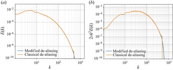
This filtering is obtained by the modification of the classical spectral cut-off filter applied, namely the  $2/3$ truncation, for de-aliasing of the pseudo-spectral method. More details concerning the reasons why the modified de-aliasing procedure was used, and how it improved the quality of the data, can be found in Appendix A along with the energy and dissipation spectra at the centreplane of the jet. For the modified de-aliasing method, a filter function
 $R(|\boldsymbol {k}|)$ (where
 $\boldsymbol {k} = (k_x, k_y, k_z)$) has been applied in the form
 $R(|\boldsymbol {k}|) = 2 - \exp (c_1(|\boldsymbol {k}| - k_{filter})^2)$, where
 $c_1$ is a coefficient chosen to fix the value
 $R(k_{cut\text {-}off}) = 0.01$. The wavenumbers with
 $|\boldsymbol {k}| < k_{filter}$ are completely unaffected from the filtering, and the wavenumbers with at least one component greater than the cut-off wavenumber, i.e.
 $\max [(k_x, k_y, k_z)] > k_{cut\text {-}off}$, are truncated. The wavenumbers with
 $|\boldsymbol {k}| > k_{filter}$ but
 $\max [(k_x, k_y, k_z)] < k_{cut\text {-}off}$ are then filtered by using the function
 $R(|\boldsymbol {k}|)$. Due to the shape of
 $R(|\boldsymbol {k}|)$, the effect of this modified de-aliasing is limited to only the wavenumbers very close to the cut-off wavenumbers, which is presented in Appendix A.
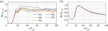
Figure 1(a) shows the Reynolds number defined in terms of the Taylor length scale  $\lambda = \sqrt {10 \nu K_0/\epsilon _0}$, where
 $K_0$ and
 $\epsilon _0$ are the kinetic energy and dissipation averaged over the centreplane (
 $\kern0.06em y = 0$). Here,
 $Re_{\lambda }=(\sqrt {2/3 K_0}\,\lambda )/ \nu$ remains constant at approximately
 $Re_\lambda \sim 45\unicode{x2013}65$ throughout the time evolution of the jet after transition to the fully turbulent regime. Given that
 $\nu /\sqrt {K_{c}} \sim \eta (\eta /\delta )^{1/3}$, the constancy of
 $Re_\lambda$ in time is one indication that the turbulent length scales of the flow evolve similarly in time as expected from the previous section. Figure 1(b) shows that at all times, the spatial resolution remains higher than the Kolmogorov length calculated in the centreplane
 $y=0$. This resolution is observed to be critical for the postprocessing in this study as it is related directly to the accurate resolution of the geometrical properties of the TNTI. Appendix B shows results from simulations conducted with higher Reynolds numbers by making a trade-off with the resolution, and demonstrates the necessity for the high grid resolution favoured in the present study.
(a) Taylor Reynolds number  $Re_\lambda$ and (b) spatial resolution
 ${\rm d}y = H_J / 128$, normalised by the Kolmogorov scale at the centreplane of the jet (
 $\kern0.06em y=0$). The five different curves correspond to our five DNS realisations.

5. Results
5.1. Self-similarity and length scales
The analysis of the DNS data starts with mean profiles in order to determine the self-similar region where the investigation of the TNTI is to be conducted. In order to determine the time when the jet becomes self-similar, mean profiles of the streamwise velocity, turbulent kinetic energy and the  $\langle u'v' \rangle$ component of the Reynolds stress are considered. Self-similarity means that statistics evolve with a time-local amplitude scaling and a time-local length scale, i.e.
 $\phi _0(t)$ and
 $\ell (t)$, so that the time-dependent
 $y$-profile of an
 $x$- and
 $z$-averaged quantity
 $\phi$ can be written in the form (Townsend Reference Townsend1976)
 \begin{equation} \phi = \phi_0(t)\,f(y / \ell (t)). \end{equation}
For the investigation of the self-similarity of the mean flow profiles, we start by normalising the profiles by using the jet half-width  $\delta (t)$ (defined as the absolute value of
 $y$, where
 $U(y)$ is
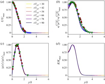
 $U(0)/2$) as time-local length scale; see figure 2. In order to distinguish between self-similarity and scaling, the profiles are normalised in figure 2 by their maxima (Dairay et al. Reference Dairay, Obligado and Vassilicos2015).
Profiles of mean streamwise velocity  $U$, streamwise velocity r.m.s.
 $u_{rms}$, Reynolds shear stress
 $\langle u'v' \rangle$, and turbulent kinetic energy
 $K$, normalized by the maximum values of the respective profiles and compared with experimental data from Cafiero & Vassilicos (Reference Cafiero and Vassilicos2019) (blue circles), Ramaprian & Chandrasekhara (Reference Ramaprian and Chandrasekhara1985) (green triangles) and Gutmark & Wygnanski (Reference Gutmark and Wygnanski1976) (red squares).

With similar DNS, da Silva & Pereira (Reference da Silva and Pereira2008) report that the self-similar regime starts at  $t/T_{ref} \approx 20$, which is after the transition to turbulence has happened. In another study of the same flow, Van Reeuwijk & Holzner (Reference Van Reeuwijk and Holzner2013) report that the jet becomes fully turbulent at
 $t/T_{ref} \approx 30$. Looking at figure 2, it is observed that the mean flow, Reynolds stress, root-mean-square (r.m.s.) streamwise velocity and turbulent kinetic energy profiles collapse rather well as functions of
 $y/\delta (t)$ for
 $t/T_{ref} \geq 30$ in the present simulations;
 $t/T_{ref} = 30$ marks the beginning of the self-similar regime, and as shown in figure 1(a), it is also when the Taylor length Reynolds number starts remaining approximately constant in time. In figure 2, the self-similar profiles are also compared with the experimental data of Gutmark & Wygnanski (Reference Gutmark and Wygnanski1976), Ramaprian & Chandrasekhara (Reference Ramaprian and Chandrasekhara1985) and Cafiero & Vassilicos (Reference Cafiero and Vassilicos2019), showing good collapse between the present data and the profiles obtained in the experiments.
Figure 3(a) shows the time evolution of the normalized square of the jet half-width, i.e.  $\delta ^2/H_J^2$.
(a) Time variation of the square of the jet half-width,  $\delta ^2$. The red dashed line is the linear fit to the data for times when the jet is fully turbulent and mean profiles are self-similar. (b) Ratios
 $\lambda / \eta$ (solid line) and
 $\delta / \lambda$ (dashed line), demonstrating the similar time evolution of all length scales of the flow.

The data plotted in figures 2 and 3(a) are ensemble averages over the five simulations (as well as averages over the  $x\unicode{x2013}z$ plane in every simulation, of course). A linear fit to the data for
 $t/T_{ref} \geq 30$ shows that
 $\delta ^2$ grows linearly with time, in agreement with the prediction in § 2. Figure 3(b) shows ratios of length scales, namely
 $\eta (t)/\lambda (t)$ and
 $\delta (t)/\lambda (t)$, where
 $\lambda$ and
 $\eta$ are calculated in terms of turbulent kinetic energy and dissipation rate at the centreplane
 $y=0$. It is observed that the turbulence length scales
 $\lambda$ and
 $\eta$ evolve similarly in time. In addition, the mean flow length scale
 $\delta (t)$ also evolves in the same way, leading to the confirmation of the conclusion in § 2 that all length scales grow identically with time.
To extract from the DNS data the scaling quantity  $R_0$ of § 2, we identify it with
 $\langle u'v'\rangle _{max}$, the maximum value of the Reynolds shear stress profile in figure 2.
We find that the Townsend assumption  $K_0 \sim R_0$ holds for times
 $t/T_{ref}=30$ to
 $t/T_{ref}=80$ (figure 3a). According to the scalings derived in § 2,
 $K_0$ should vary in time like
 $u_{0}^{2}$, where
 $u_{0} (t) \equiv U(y=0,t)$, and this is confirmed by our DNS data, as figure 4(a) makes clear over a range of times even greater than
 $K_0 \sim R_0$ (up to
 $t/T_{ref} =100$). This range of times is greater because the effects of the boundary conditions on the time-developing jet appear to be felt first by the Reynolds shear stress and later by other quantities such as
 $K_0$ and
 $u_0$. We chose to process our data from
 $t/T_{ref}=30$ to
 $t/T_{ref}=100$, where self-similarity holds and where the constancy of
 $u_0 \delta$, related to the volume flux (2.6), is definitely respected in our DNS (figure 4b). With the exception of figure 4(a) where
 $K_{0}/R_{0}$ starts deviating from its constancy in time after
 $t/T_{ref}=80$, all the figures where we plot quantities versus time do not show a drastic change after
 $t/T_{ref}=80$, which is why we chose to process our data until
 $t/T_{ref}=100$ rather than
 $t/T_{ref}=80$. There is no effect on our paper's conclusions.
(a) The ratios  $K_0/R_0$ and
 $K_0/u_0^2$, and (b) constancy of the normalised volume flux, between
 $t/T_{ref}=26$ and
 $t/T_{ref}=98$.

5.2. Time dependence of scaling parameters and virtual origin
The time dependencies of the centreline streamwise velocity scale  $u_0(t)$ and of the jet half-width
 $\delta (t)$, (2.19) and (2.20), are found to be power laws
 \begin{equation} \phi(t) = A(t - t_0)^b \end{equation}
in the theoretical analysis of § 2. It is important to note that these two power laws must combine properly to satisfy the governing equations, and that this can happen only if the virtual origin  $t_0$ is the exact same one in (2.19) and (2.20) (Nedić Reference Nedić2013; Nedić, Vassilicos & Ganapathisubramani Reference Nedić, Vassilicos and Ganapathisubramani2013; Dairay et al. Reference Dairay, Obligado and Vassilicos2015; Cafiero & Vassilicos Reference Cafiero and Vassilicos2019).
There exist various methods for the determination of the exponent  $b$ while taking proper account of the virtual origin
 $t_0$ (Nedić et al. Reference Nedić, Vassilicos and Ganapathisubramani2013; Dairay et al. Reference Dairay, Obligado and Vassilicos2015; Cafiero & Vassilicos Reference Cafiero and Vassilicos2019). In the present study, the method used in Cafiero & Vassilicos (Reference Cafiero and Vassilicos2019) is implemented on
 $u_{0}(t) \sim (t-t_{0})^b$ and
 $\delta (t) \sim (t-t_{0})^{-b}$.
The procedure starts with initial fits to the  $u_0$ data in the form
 $u_0 \sim t^b$, and to the
 $\delta$ data in form
 $\delta \sim t^{-b}$, in agreement with volume flux conservation, (2.6). By this step, two approximate values for the exponent
 $b$ are obtained as initial guesses. Then the value of the exponent is varied in a certain range around the initial guess in order to find the corresponding
 $t_0$ values for every value of
 $b$. This procedure is carried out for both
 $u_0$ and
 $\delta$ separately. Plotting the resulting
 $(b, t_0)$ pairs yields the plot in figure 5, where blue and red colours are differentiating the values obtained from the
 $u_0$ and
 $\delta$ data. At the point where these two lines intersect, the best fit values
 $(b, t_0)$ are the ones that take into account that the virtual origin must be identical for both
 $u_0$ and
 $\delta$. These values are
 $b=-0.51$ and
 $t_0 = 11.7$. The time evolutions of
 $u_0$ and
 $\delta$ in the time range
 $t/T_{ref} = 30$ to
 $/T_{ref} = 100$, and their power-law fits with the pair
 $b = -0.51$,
 $t_0 = 11.7$, are shown in figure 6.
The optimal virtual origin  $t_0$ as a function of exponent
 $b$ for the time evolutions of
 $u_0$ (blue circles) and
 $\delta$ (red squares). The dashed vertical lines show the best fit exponent
 $b$ for
 $t_0 = 0$ (blue for
 $u_0$, red for
 $\delta$), and the green diamond marks the one value of
 $b$ for which
 $t_0$ is the same for both (2.19) and (2.20).

Time variation of (a)  $u_0$ and (b)
 $\delta$, with the best power-law fits obtained by the procedure based on figure 5.

At this point, we recall our result of § 2 that, unlike spatially developing turbulent jets (Cafiero & Vassilicos Reference Cafiero and Vassilicos2019), the evolutions (in time) of  $u_0$ and
 $\delta _0$ in temporally developing turbulent jets are independent of the exponent
 $m$ in the turbulence dissipation law (2.18). The values found for
 $b$ and
 $t_0$ from the DNS data are compatible with the theoretical value
 $b=-0.5$ obtained in § 2 for any exponent
 $m$.
5.3. Identification of the turbulent jet and locating the TNTI
The TNTI is associated with the very high gradients of enstrophy observed between the rotational turbulent region and the irrotational outer flow. Thus it is the layer where isosurfaces of very different enstrophy values are spatially stacked very close to each other. In figure 7, we plot the turbulent jet volume  $V_J$, defined as the volume where
 ${\omega }^{2} \geq \omega _{th}^{2}$, where
 ${\omega }^{2}$ is the enstrophy of the fluctuating velocity field, and
 $\omega _{th}^{2}$ is a threshold enstrophy. In this figure,
 $V_J$ is normalised by the domain volume
 $V_{tot}$, and plotted versus the normalised enstrophy threshold values
 $\omega ^2_{th}/\omega ^2_{ref}$, where the reference enstrophy
 $\omega _{ref}^{2}$ is the mean enstrophy value averaged over the centreplane. (Note that
 $\omega _{ref}^{2}$ evolves in time.)
Detected turbulent volume  $V_J/V_{tot}$ obtained by varying the threshold values
 $\omega ^2_{th}/\omega ^2_{ref}$ for one of the simulations (PJ1).

Figure 7 reveals the presence of a plateau over a very wide range of threshold values at any time between  $t/T_{ref}=30$ and
 $t/T_{ref}=90$. This is the range of enstrophies packed tightly together within the TNTI, leading to
 $V_J/V_{tot}$ being approximately constant for a wide range of
 $\omega ^2_{th}/\omega ^2_{ref}$ values, and thereby reflecting the sharp demarcation between the turbulent region and the outer non-turbulent region. Starting from the turbulent side of the TNTI and going through the interface, the enstrophy drops rapidly from its nearly homogeneous non-zero value in the inner region of the jet towards zero within a very short distance, which is typically of the order of
 $10\eta$ for the Reynolds numbers reachable by current DNS (Nagata, Watanabe & Nagata Reference Nagata, Watanabe and Nagata2018; Silva et al. Reference Silva, Zecchetto and da Silva2018).
The left-hand side of the plateau, corresponding to low enstrophy threshold values, is limited by the numerical noise. These numerical oscillations get significant as the threshold value goes to zero. The additional filtering that we introduced to reduce the numerical oscillations increases the  $\omega ^2_{th}/\omega ^2_{ref}$ range of the plateau by extending its left-hand side to values closer to
 $\omega ^2_{th}/\omega ^2_{ref} = 0$, as the outer edge of the TNTI is cleaner in terms of noise.
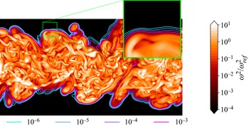
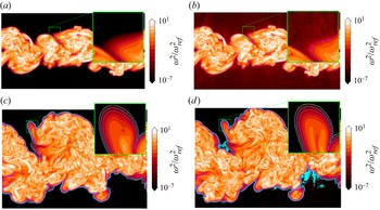
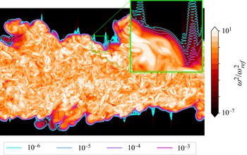
Figure 8 shows a part of the computational domain that includes the turbulent jet for PJ1 at  $t/T_{ref}=50$. The inset is the magnification of a small region around the TNTI and shows the isocontours
 $\omega ^2_{th}/\omega ^2_{ref} = 10^{-6}, 10^{-5}, 10^{-4}, 10^{-3}$. These threshold values are within the enstrophy range of the plateau in figure 7 and are therefore within the TNTI. Surfaces that are clean in terms of noise can be obtained for a very wide range of enstrophy thresholds from the simulation data.
Contour field of  $\omega ^2/\omega ^2_{ref}$ and isocontours of certain
 $\omega ^2_{th}/\omega ^2_{ref}$ values to mark the TNTI layer. Simulation PJ1 at
 $t/T_{ref}=50$.

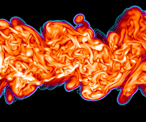
Following the determination of the  $\omega ^2_{th}/\omega ^2_{ref}$ range defining the TNTI, we now determine the TNTI as shown in figure 9. The procedure starts by labelling the turbulent volume by the condition
 $\omega ^2(x,y,z) \ge \omega ^2_{th}/\omega ^2_{ref}$, and obtaining the binary field. The turbulent region corresponds to the blue region in figure 9(a), and the non-turbulent regions correspond to the white and red marked regions, where the engulfed regions (shown with red) are still present. Following this, the non-turbulent volumes are labelled in three dimensions by using the labelling function from the open-source SciPy library (Virtanen et al. Reference Virtanen2020), so that all independent non-turbulent volumes have their individual label number. At this stage, the connectivities of the non-turbulent regions are checked, leading to detection of engulfed non-turbulent volumes (with no connection in three dimensions with the external irrotational region). Some examples of these detected engulfed volumes can be seen in figure 9(a), marked in red. The white detached regions inside the turbulent area of figure 9(a) (in blue) are connected to the outer non-turbulent region in the three-dimensional field (out of the figure's plane). In order to consider only the outer surface, the engulfed volumes are suppressed in this study. To get the surface corresponding to a chosen
 $\omega ^2_{th}/\omega ^2_{ref}$ in three dimensions, a dilation procedure is used in three dimensions to expand the non-turbulent region into the turbulent region. Then by subtracting the original field from the dilated field, we end up with a field where the three-dimensional jet envelope is marked by the number 1, and all other data points are marked 0 in the entire simulation domain. A cut-section of the resulting field is shown in figure 9(b), as the dark line. This detection procedure is applied for various enstrophy threshold values to obtain the interface characteristics at different locations throughout the TNTI layer as in Van Reeuwijk & Holzner (Reference Van Reeuwijk and Holzner2013) and Krug et al. (Reference Krug, Chung, Philip and Marusic2017).
(a) The labelling of the turbulent, non-turbulent and engulfed regions. (b) Detected TNTI. For the instant  $t/T_{ref}=50$ of simulation PJ1,
 $\omega ^2_{th}/\omega ^2_{ref} = 10^{-3}$.

5.4. Fractal dimensions of the TNTI
The theoretical analysis in § 2 relates the fractal dimension of the TNTI to the global Reynolds number scaling of the TNTI propagation velocity; see (3.6). It is therefore important to investigate the fractal/fractal-like properties of the TNTI.
The fractal/fractal-like nature of scalar isosurfaces relating to the TNTI has been reported in various studies (Sreenivasan et al. Reference Sreenivasan, Ramshankar and Meneveau1989; Miller & Dimotakis Reference Miller and Dimotakis1991; Sreenivasan Reference Sreenivasan1991; Lane-Serff Reference Lane-Serff1993; Dimotakis & Catrakis Reference Dimotakis and Catrakis1999; Mistry et al. Reference Mistry, Philip, Dawson and Marusic2016; Mistry, Dawson & Kerstein Reference Mistry, Dawson and Kerstein2018). However, these fractal/fractal-like characteristics are described somewhat differently in different studies. In some studies, a well-defined power law for the scale dependence of the surface area (thus constant fractal dimension) has been reported (Sreenivasan et al. Reference Sreenivasan, Ramshankar and Meneveau1989; Sreenivasan Reference Sreenivasan1991; Mistry et al. Reference Mistry, Philip, Dawson and Marusic2016, Reference Mistry, Dawson and Kerstein2018). This is the case where, when one covers the surface with boxes of size  $r$, the number
 $N$ of boxes needed to fully cover the surface scales as
 $N(r) \sim r^{-D_f}$ (Mandelbrot Reference Mandelbrot1982), and the fractal dimension
 $D_f$ of the surface is independent of
 $r$ over a significant range of scales
 $r$. In other studies of isosurfaces, in flows such as turbulent jets and mixing layers, a scale-dependent fractal dimension is reported, i.e.
 $D_{f} = D_{f}(r)$, which means that there is no constant value for the fractal dimension
 $D_f$, but the fractal dimension varies with box size
 $r$ (Miller & Dimotakis Reference Miller and Dimotakis1991; Dimotakis & Catrakis Reference Dimotakis and Catrakis1999; Catrakis & Dimotakis Reference Catrakis and Dimotakis1999).
There is also the question of the enstrophy threshold used to define the TNTI because a strong threshold dependence of the fractal dimension of scalar isosurfaces has been reported in some studies (Miller & Dimotakis Reference Miller and Dimotakis1991; Lane-Serff Reference Lane-Serff1993; Flohr & Olivari Reference Flohr and Olivari1994). Varying the threshold within the range of thresholds where  $V_J$ remains approximately constant is akin to sampling different inner iso-enstrophy surfaces within the TNTI layers’ inner structure (Van Reeuwijk & Holzner Reference Van Reeuwijk and Holzner2013). There may be not one single fractal dimension for the TNTI, but different fractal dimensions for different inner isosurfaces of enstrophy within the TNTI layer, an aspect of the problem that needs to be investigated.
We apply the box-counting procedure to obtain fractal dimensions of iso-enstrophy surfaces within the TNTI. Figure 10 shows typical ensemble-averaged box-counting results, these particular ones being for the isosurface  $\omega ^2_{th}/\omega ^2_{ref} = 10^{-3}$ at time
 $t/T_{ref}=50$. Figure 10(a) is a log–log plot of the number
 $N$ of boxes needed to cover the iso-enstrophy surface versus the inverse box size
 $1/r$. The linear fit in orange is obtained by using all the points on the plot, and the slope of this fit is found to be
 $D_{f1}=2.161$ for this particular case. On the other hand, local slopes are also calculated by fits over nine consecutive data points on this plot. It is observed (see the example in figure 10b) that the local slope does not remain constant throughout all scales
 $r$. An approximately constant fractal dimension, seen as a plateau-like region in figure 10(b), appears to exist between
 $r = \delta$ and
 $r = \lambda$ for the entire range of isosurfaces of various enstrophy threshold values within the TNTI (
 $\omega _{th}^{2}/\omega ^2_{ref}$ between
 $10^{-6}$ and
 $10^{-3}$) and for all times where the jet is fully turbulent (local slope values marked by red square markers). Note that the constancy of this local fractal dimension is affected by the fact that it is calculated by using nine points around the value of
 $r$ where the local dimension is evaluated. This means that the highly non-constant values of the fractal dimension at scales
 $r$ larger than
 $\delta$ are responsible for deviations from constancy at scales close to but below
 $\delta$, and that the progressive decrease of the local slope towards
 $D_f =2$ as
 $r$ decreases at scales
 $r$ below
 $\lambda$ is responsible for the systematic deviation from constancy at scales close to yet larger than
 $\lambda$.
Ensemble-averaged results of the box-counting method applied to isosurface  $\omega ^2_{th}/\omega ^2_{ref} = 10^{-3}$ at time
 $t/T_{ref} = 50$. (a) A plot of the number of boxes
 $N$ of size
 $r$ versus
 $1/r$ is shown in log–log scale, the orange line being the linear best fit for all data points on this plot. (b) The local slope calculated by the fits using nine consecutive data points, the value of the local slope being attributed to the centre point. The local slopes marked as red squares (as opposed to blue circles) are the points used to calculate
 $D_{f2}$. The dashed, dot-dashed and dotted vertical lines locate on the horizontal axis the length scales
 $\delta$,
 $\lambda$ and
 $\eta$, respectively (where
 $\lambda$ and
 $\eta$ are calculated on the centreplane.)

Throughout this study, the fractal dimension is calculated as the average value of the local slopes between box sizes  $r = \delta$ and
 $r = \lambda$, and this fractal dimension is denoted
 $D_{f2}$. The first point with
 $r$ smaller than or equal to
 $\delta$ (i.e. the largest value of
 $r$ in the range
 $\lambda \leq r \leq \delta$) is excluded from this average so as to reduce the oscillation caused by less-converged values of
 $N$ at larger box sizes.
The fractal dimension  $D_{f2}$ for different enstrophy threshold values in the TNTI range
 $\omega _{th}^2/\omega _{ref}^2\in [ 10^{-6}, 10^{-3}]$ is shown in figure 11 as a function of time. The fractal dimensions
 $D_{f2}$ of the TNTI may be considered to remain approximately constant in time for all these enstrophy thresholds, and the mean value around which
 $D_{f2}$ appears to fluctuate is shown by the dashed lines in the figure. For the threshold values
 $\omega _{th}^2/\omega _{ref}^2\in [ 10^{-6}, 10^{-3}]$, this fractal dimension value varies from
 $D_{f2}=2.09$ to
 $D_{f2}=2.18$. It can be observed that the values of
 $D_{f2}$ for different
 $\omega ^2_{th}/\omega ^2_{ref}$ get closer to each other towards the lower values of
 $\omega ^2_{th}/\omega ^2_{ref}$. It can also be argued that an objective definition of the viscous superlayer must include, within the superlayer, enstrophy iso-values for which the fractal dimension can be detected with a value larger than 2.
TNTI fractal dimensions  $D_{f2}$ versus time
 $t/T_{ref}$ for different normalised enstrophy thresholds within the TNTI.

A significantly higher value,  $D_{f2} = 2.36$, has been observed for the iso-enstrophy surface defined by the threshold
 $\omega _{th}^2/\omega _{ref}^2=10^{-2}$. This value is close to the fractal dimension
 $7/3 \approx 2.33$ reported in various studies (Sreenivasan et al. Reference Sreenivasan, Ramshankar and Meneveau1989; Sreenivasan Reference Sreenivasan1991; Mistry et al. Reference Mistry, Philip, Dawson and Marusic2016, Reference Mistry, Dawson and Kerstein2018). It must be noted that the enstrophy threshold
 $\omega _{th}^2/\omega _{ref}^2=10^{-2}$ rests on the turbulent side of the TNTI judging from the enstrophy range of the plateau shown in figure 7. However, it is also observed that the
 $\log _2 N$–
 $\log _2(1/r)$ plot obtained from the box-counting algorithm for this enstrophy threshold shows no evidence of a fractal dimension that is independent of
 $r$, i.e. there is no significant plateau region in figure 12(b), and the local slope varies significantly with
 $r$. The value
 $D_{f2} = 2.36$ is obtained by averaging over the local fractal dimensions (local slopes in figure 12b) from
 $r=\lambda$ to
 $r=\delta$, but these local fractal dimensions vary continuously with
 $r$ from 2.2 to over 2.45.
Same as figure 10, but for iso-enstrophy surface  $\omega ^2_{th}/\omega ^2_{ref} = 10^{-2}$ at the same time
 $t/T_{ref} = 50$.

5.5. Propagation velocity of the interface
In § 2, we obtained (3.6) for the TNTI's mean propagation velocity on the basis of the fractal/fractal-like character of the TNTI. We now know, following the previous subsection, that the TNTI of our time-developing turbulent jet has a range of fractal dimensions  $D_{f2}$ depending on the normalised enstrophy threshold
 $\omega _{th}^{2}/\omega _{ref}^{2}$, and that
 $D_{f2}$ is a fairly well-defined single number independent of box size
 $r$ in the range
 $\lambda \le r\le \delta$ if
 $\omega _{th}^{2}/\omega _{ref}^{2}$ is in the range
 $[ 10^{-6}, 10^{-3}]$. The question that arises naturally now is: Does (3.6) capture the time and enstrophy-threshold dependencies of the mean propagation velocity
 $v_n$? More specifically, can we use
 $D_{f2} = D_{f2} (\omega _{th}^{2}/\omega _{ref}^{2})$ defined in the range
 $\lambda \le r\le \delta$ as the fractal dimension in (3.6) to capture accurately the time and enstrophy-threshold dependencies of
 $v_n$? We stress that in this formula,
 $v_n$ depends on the enstrophy threshold only through
 $D_{f2}$, given that
 $A$ is defined in terms of quantities that are independent of enstrophy threshold, and
 $a$ in
 $V_{J}=2a\delta L_{x}L_{z}$ can be expected to have a negligibly weak dependence on enstrophy threshold.
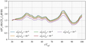
To estimate  $v_n$ independently from (3.6), we use (3.2), having first checked the validity of
 ${{\rm d}V_{J}}/{{\rm d}t} = 2a L_{x}L_{z}\,({{\rm d} \delta }/{{\rm d}t})$ (see figure 13), which is needed to go from (3.1) to (3.2). Figure 13 confirms that the dimensionless coefficient
 $a$ is approximately independent of time as it oscillates around the constant value
 $a=1.66$, and that it is also very weakly dependent on enstrophy threshold over at least four decades.
Validity of  ${{\rm d} V_{J}}/{{\rm d}t} \sim 2 L_{x}L_{z}\,({{\rm d} \delta }/{{\rm d}t})$ over the time evolution of the fully turbulent jet.

To use (3.2), we need a reliable estimate of the TNTI surface area  $S$ that is different from the fractal estimate (3.3). To obtain such an estimate of
 $S$, we plot
 $r^{2}\,N(r)$: as the box-counting algorithm's box size
 $r$ decreases and becomes small enough to resolve all the contortions of the iso-enstrophy surface,
 $r^{2}\,N(r)$ reaches a maximum and does not grow further with further decreasing
 $r$. We take this maximum as our estimate of
 $S$, i.e.
 $S=S_{R}\equiv \max _{r}[r^{2}\,N(r)]$. Of course,
 $S$ depends on the enstrophy threshold defining the chosen isosurface within the TNTI, and figure 14(a) shows an example of an
 $r^{2}\,N(r)$ versus
 $1/r$ log–log plot for
 $\omega _{th}^{2}/\omega _{ref}^{2} = 10^{-3}$ at
 $t/T_{ref}=50$, where the maximum
 $r^{2}\,N(r)$ is reached at
 $r$ close to
 $\eta$. In fact, figure 14(a) is quite typical of normalised enstrophy thresholds in the range
 $[ 10^{-6}, 10^{-3}]$ and times
 $t/T_{ref}$ in the range
 $[ 30, 100 ]$.
(a) Plot (using  $\log _{2}$ values) of
 $r^{2}\,N (r)$ versus
 $1/r$, at time
 $t/T_{ref}=50$, for the threshold value
 $\omega _{th}^2/\omega _{ref}^2=10^{-3}$. The horizontal dashed line indicates the maximum value of
 $r^{2}\,N (r)$. (b) Plot of
 $S_{R}/(L_{x}L_{z}) \equiv \max _{r}[r^{2}\,N(r)]/(L_{x}L_{z})$ versus time
 $t/T_{ref}$ for different enstrophy threshold values.

In figure 14(b), we plot  $S_{R}\equiv \max _{r}[r^{2}\,N(r)]$ as a function of
 $t/T_{ref}$ for various normalised enstrophy thresholds. Interestingly, the TNTI surface areas
 $S_R$ remain approximately constant in time for all thresholds
 $\omega _{th}^2/\omega _{ref}^2=10^{-6}$ to
 $10^{-4}$ from
 $t/T_{ref} = 40$ to
 $100$, and for threshold
 $\omega _{th}^2/\omega _{ref}^2=10^{-3}$ from
 $t/T_{ref} = 50$ to
 $100$. This is compatible with the fact that all length scales, large and small, grow together in this flow.
We now calculate the average TNTI propagation velocity  $v_n$ by using (3.2) with
 $S$ obtained from
 $S_{R}\equiv \max _{r}[r^{2}\,N(r)]$, and we compare it with (3.6). First, in figure 15 we check the time-dependence of
 $v_n$, which, according to (3.6) and
 $\delta \sim \sqrt {U_{J}H_{J}(t-t_{0})}$, is the same as the time dependence of
 $u_{\eta }$ and of
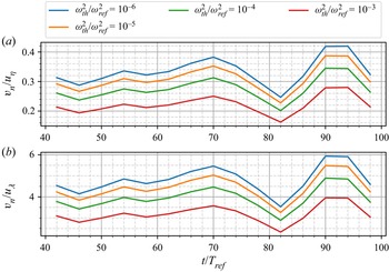
 $u_{\lambda }$. In support of this prediction, figure 15 shows that
 $v_{n}/u_{\eta }$ and
 $v_{n}/u_{\lambda }$ oscillate around a constant as time proceeds for all
 $\omega _{th}^{2}/\omega _{ref}^{2}$ in the range
 $[ 10^{-6}, 10^{-3}]$.
Time dependence of (a)  $v_{n}/u_{\eta }$ and (b)
 $v_{n}/u_{\lambda }$.

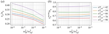
Second, we check the enstrophy threshold dependence of  $v_n$, which, according to (3.6), should be
 $v_{n}/u_{\eta } \sim (Aa)^{1/(D_{f}(\omega _{th}^{2}/\omega _{ref}^{2})-1)} Re_{G}^{[2-D_{f}(\omega _{th}^{2}/\omega _{ref}^{2})]/[D_{f}(\omega _{th}^{2}/\omega _{ref}^{2})-1] +1/4}$ and equivalently
 $v_{n}/u_{\lambda } \sim (Aa)^{1/(D_{f}(\omega _{th}^{2}/\omega _{ref}^{2})-1)} Re_{G}^{[2-D_{f}(\omega _{th}^{2}/\omega _{ref}^{2})]/[D_{f}(\omega _{th}^{2}/\omega _{ref}^{2})-1] +1/2}$. We plot
 $v_{n}/u_{\eta }$ versus
 $\omega _{th}^{2}/\omega _{ref}^{2}$ for various time instants
 $t/T_{ref}$ in figure 16(a); and we take our measured
 $D_{f2} (\omega _{th}^{2}/\omega _{ref}^{2})$ (averaged over time for simplicity, this average being denoted
 $\overline {D_{f2}}$) to represent the fractal dimension
 $D_f$, and plot
 $(v_{n}/u_{\eta })(Aa)^{-1/(\overline {D_{f2}}-1)} Re_{G}^{-(2-\overline {D_{f2}})/(\overline {D_{f2}}-1)}$ versus
 $\omega _{th}^{2}/\omega _{ref}^{2}$ for various time instants
 $t/T_{ref}$ in figure 16(b). If (3.6) is able to capture the enstrophy threshold dependence of
 $v_n$, then
 $(v_{n}/u_{\eta })(Aa)^{-1/(\overline {D_{f2}}-1)} Re_{G}^{-(2-D_{f2})/(D_{f2}-1)}$ should be constant with varying
 $\omega _{th}^{2}/\omega _{ref}^{2}$ for all times
 $t/T_{ref}$ between
 $30$ and
 $100$, with
 $a \approx 1.66$ (as found already from figure 13) and
 $A\approx 0.058$ from figure 3(a).
(a) Average interface propagation velocity  $v_n$ normalised by
 $u_\eta$ versus normalised enstrophy threshold for different times
 $t/T_{ref}$. (b) Plot of
 $v_n$ divided by
 $(Aa)^{1/(\overline {D_{f2}}-1)}Re_{G}^{(2-\overline {D_{f2}})/(\overline {D_{f2}}-1)}$ according to (3.6) (with
 $A=0.05777$ and
 $a=1.6574$) normalised by
 $u_\eta$ versus normalised enstrophy threshold for different times
 $t/T_{ref}$.

We can see clearly in figure 16(a) that, irrespective of time,  $v_n$ decreases with increasing
 $\omega _{th}^{2}/\omega _{ref}^{2}$ in the TNTI normalised enstrophy range
 $[ 10^{-6}, 10^{-3}]$, which makes sense because
 $S$ increases with increasing
 $\omega _{th}^{2}/\omega _{ref}^{2}$. Indeed, we expect
 $Sv_n$ to be approximately independent of
 $\omega _{th}^{2}/\omega _{ref}^{2}$ in the TNTI range of enstrophy thresholds, judging from (3.1) and the approximate constancy of
 $V_J$ in that range (shown in figure 7).
Figure 16(b) shows that our formula (3.6) for the TNTI's mean propagation velocity  $v_n$ with
 $D_f$ given by
 $\overline {D_{f2}}(\omega _{th}^{2}/\omega _{ref}^{2})$ – i.e. the time-averaged (from
 $t/T_{ref}=30$ to
 $98$) value of
 $D_{f2}(\omega _{th}^{2}/\omega _{ref}^{2})$ – captures the enstrophy threshold dependence of
 $v_n$ very well over the wide range of thresholds
 $10^{-6}\le \omega _{th}^{2}/\omega _{ref}^{2} \le 10^{-3}$, which is within the TNTI throughout the time range considered.
In the next section we explore the inconsistencies of the simple fractal model for  $v_n$ presented in § 2, and investigate how they might be overcome.
5.6. A generalised Corrsin length for the TNTI
Our simple fractal model's formula (3.6) predicts quite well both the time dependence of the TNTI's mean propagation velocity  $v_n$ and its enstrophy threshold dependence. However, our fractal model did not foresee the complex inner structure of the TNTI where different iso-enstrophy surfaces within the TNTI have different fractal dimensions.
Our model is based on: (i)  ${{\rm d} V_{J}}/{{\rm d}t}= 2a L_{x}L_{z}\,({{\rm d}\delta }/{{\rm d}t})$ (needed to go from (3.1) to (3.2)), which our simulations rather support (see figure 13); (ii)
 $S = L_{x}L_{z} (\eta _{I}/\delta )^{2-D_{f}}$, where
 $\eta _{I} = \nu /v_{n}$ is the Corrsin length scale for the viscous superlayer's thickness; and (iii) a well-defined fractal dimension
 $D_f$ independent of
 $r$ over a significant range of
 $r$ values bounded from below by the smallest length scale on the TNTI. In the event, our DNS data have returned well-defined fractal dimensions
 $D_{f2}$ independent of
 $r$ in a range bounded from below by
 $\lambda$ but not by the smallest length scale on the TNTI, which appears to be
 $\eta$ as the maximum of
 $r^{2}\,N(r)$ is typically reached at
 $r$ close to
 $\eta$. The number
 $N$ of boxes needed to cover iso-enstrophy surfaces continues to increase faster than
 $r^{-2}$ as
 $r$ decreases from
 $\lambda$ to
 $\eta$, implying that these scales between
 $\lambda$ and
 $\eta$ contribute to the surface area, but not with a well-defined
 $r$-independent fractal dimension. Furthermore, in the range where an
 $r$-independent fractal dimension may be claimed, i.e.
 $\lambda \le r\le \delta$, this fractal dimension
 $D_{f2}$ is a decreasing function of enstrophy threshold
 $\omega _{th}^{2}/\omega _{ref}^{2}$, appearing to tend towards close to 2 as
 $\omega _{th}^{2}/\omega _{ref}^{2}$ tends to
 $0$.
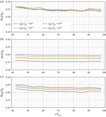
In figure 17, we plot  $S(\eta ) = L_{x}L_{z}(\eta /\delta )^{2-D_{f2}}$,
 $S(\lambda ) = L_{x}L_{z}(\lambda /\delta )^{2-D_{f2}}$ and
 $S(\eta _{I}) = L_{x}L_{z}(\eta _{I}/\delta )^{2-D_{f2}}$, all normalised by
 $S_{R}\equiv \max _{r}[r^{2}\,N(r)]$. These three quantities are plotted versus time for different enstrophy thresholds within the TNTI range of thresholds, i.e.
 $\omega _{th}^{2}/\omega _{ref}^{2}$ within
 $[ 10^{-6}, 10^{-3}]$. The fractal dimension
 $D_{f2}$ is our only possible choice of fractal dimension for the calculations of
 $S(\eta )$,
 $S(\lambda )$ and
 $S(\eta _{I})$ if we want to be consistent with our model's requirement that the fractal dimension should be well defined, i.e.
 $r$-independent over a significant
 $r$ range.
Plots of (a)  $S(\eta ) = L_{x}L_{z}(\eta /\delta )^{2-D_{f2}}$, (b)
 $S(\lambda ) = L_{x}L_{z}(\lambda /\delta )^{2-D_{f2}}$ and (c)
 $S(\eta _{I}) = L_{x}L_{z}(\eta _{I}/\delta )^{2-D_{f2}}$ (where
 $\eta _{I} = \nu /v_{n}$, with
 $v_n$ values calculated in § 5.5), all normalised by
 $S_{R}\equiv \max _{r}[r^{2}N(r)]$, versus time
 $t/T_{ref}$ for various enstrophy thresholds within the TNTI.

First, figure 17 shows that  $S(\eta )/S_R$,
 $S(\lambda )/S_R$ and
 $S(\eta _{I})/S_R$ are approximately constant in time for all TNTI enstrophy thresholds, which is not surprising given the approximate time constancies of
 $D_{f2}$ and
 $S_R$ and given that
 $\eta$,
 $\lambda$ and
 $\eta _{I}$ all have the same time dependence as
 $\delta$. Second, figure 17 shows that only
 $S(\eta )/S_R$ collapses for all enstrophy thresholds. This is not a trivial result because
 $S(\eta )$ is calculated in terms of a fractal dimension
 $D_{f2}$ that is not well-defined at scale
 $\eta$. The worse collapse is returned by
 $S(\lambda )/S_R$; and
 $S(\eta _{I})/S_R$ tends towards
 $S(\eta )/S_R$ with decreasing
 $\omega _{th}^{2}/\omega _{ref}^{2}$, which makes some sense because, in this limit,
 $D_{f2}$ decreases towards values close to
 $2$, and
 $\eta _{I}/\eta$ therefore approaches a value of order 1, extremely weakly dependent on
 $\omega _{th}^{2}/\omega _{ref}^{2}$ (see § 2). However,
 $S(\eta _{I})/S_R$ takes values between
 $1/5$ and
 $1/4$, which is different from 1 and therefore contradicts (3.5), which is a premise of our model. In fact, there is a dimensionless coefficient
 $b$ in (3.3), i.e.
 $S(r) = b L_{x}L_{z} (r/\delta )^{2-D_{f}}$. This coefficient
 $b$ is independent of enstrophy threshold because it is set by
 $S(r=\delta ) = bL_{x}L_{z}$. The only way to retrieve (3.5) is by writing
 $S=bL_{x}L_{z} (c\eta _{I}/\delta )^{2-D_{f}}$ with
 $bc^{2-D_{f}}=1$, which requires that the dimensionless coefficient
 $c$ is a function of
 $\omega _{th}^{2}/\omega _{ref}^{2}$. Without the arbitrary condition
 $bc^{2-D_{f}}=1$, the formula (3.6) predicted by our simple fractal model should be replaced by
 \begin{equation} \frac{v_n}{U_{J}}= \left(\frac{c^{D_{f}-2}}{b}\right)^{1/(D_{f}-1)}\left(Aa\right)^{1/(D_{f}-1)}\,\frac{H_J} {\delta}\, Re_G^{-(D_f -2)/(D_f-1)}. \end{equation}
The quantity  ${c^{D_{f}-2}}/{b}$ is in fact the ratio
 $S(\eta _{I})/S_{R}$ (with
 $S(\eta _{I})$ given by
 $L_{x}L_{z}(\eta _{I}/\delta )^{2-D_{f2}}$) that we plot in figure 17, and from our data it transpires that
 $(S(\eta _{I})/S_{R})^{1/(\overline {D_{f2}}-1)}$ is a significantly decreasing function of
 $\omega _{th}^{2}/\omega _{ref}^{2}$ (see figure 18). Without setting
 ${c^{D_{f}-2}}/{b} =1$, our model does not return the right enstrophy threshold dependence of
 $v_n$, and
 ${c^{D_{f}-2}}/{b} =1$ does not agree with our DNS data, which show that
 $S(\eta _{I})/S_{R}$ (with
 $S(\eta _{I})$ given by
 $L_{x}L_{z}(\eta _{I}/\delta )^{2-D_{f2}}$) takes values between
 $1/5$ and
 $1/4$. We therefore need to explore how our model could be modified to be more realistic, and we do this by generalising the Corrsin length.
Plot of  $(S(\eta _{I})/S_{R})^{1/(\overline {D_{f2}}-1)}$ as a function of
 $\omega _{th}^{2}/\omega _{ref}^{2}$ at different times
 $t/T_{ref}$.

The Corrsin length may be considered appropriate only for the viscous superlayer at the very lowest enstrophy thresholds where the generation of vorticity is viscosity-dominated and, consistently,  $S(\eta _{I})/S_R$ and
 $S(\eta )/S_R$ appear to take similar values. To generalise this property to higher enstrophy thresholds, we introduce a generalised Corrsin length
 \begin{equation} \eta_T = \nu_T / v_n \end{equation}
in terms of a local turbulent viscosity  $\nu _T$ (local to every iso-enstrophy surface within the TNTI) such that
 \begin{equation} S = b L_{x}L_{z} (c \eta_{T}/\delta)^{2-D_{f2}}, \end{equation}
where  $b$ and
 $c=c (Re_{G}, \omega _{th}^{2}/\omega _{ref}^{2})$ are dimensionless coefficients independent of time.
The simple physical idea behind (5.4) is that the process of enstrophy production is increasingly dominated by vortex stretching rather than viscosity as the enstrophy threshold increases from the outer, viscous superlayer side of the TNTI to its inner, turbulent side. Studies over the past two decades have indeed shown that the TNTI has an inner structure that includes a viscous superlayer and a sort of buffer layer or turbulent sublayer where vorticity production dominates (da Silva et al. Reference da Silva, Hunt, Eames and Westerweel2014; Taveira & da Silva Reference Taveira and da Silva2014; Nagata et al. Reference Nagata, Watanabe and Nagata2018). Hence the turbulence viscosity  $\nu _{T}=\nu _{T}(\omega ^2_{th}/\omega ^2_{ref})$ is expected to increase and become independent of the fluid's kinematic viscosity
 $\nu$ with increasing
 $\omega _{th}^{2}/\omega _{ref}^{2}$ within the TNTI.
We now ask whether (5.4), (5.5) and (3.2), which represent an attempt to improve the model for  $v_n$ in § 2, are consistent with the requirement that
 $\nu _T$ must increase with
 $\omega ^2_{th}/\omega ^2_{ref}$. The three equations just mentioned imply
 \begin{equation} \nu_{T} = \frac{2a\delta}{c}\,\frac{{\rm d} \delta}{{\rm d}t} \left( \frac{S}{bL_x L_z} \right)^{-(D_{f2}-1)/(D_{f2}-2)}, \end{equation}
where the dimensionless constant  $a$ is the one in
 $Sv_{n}=2aL_{x}L_{z}\,{\rm d}\delta /{\rm d}t$. It can be seen that
 $\nu _T$ depends on
 $\omega _{th}^{2}/\omega _{ref}^{2}$ through
 $S$ and
 $D_{f2}$ (and also
 $c$), but does not depend on time, in agreement with our observations in figures 3(a), 14(b) and 11. As
 $S/L_{x}L_{z}$ increases whereas
 $(D_{f2}-1)/(D_{f2}-2)$ decreases with increasing
 $\omega _{th}^{2}/\omega _{ref}^{2}$, it is not trivial to predict how
 $({S}/{L_x L_z})^{-(D_{f2}-1)/(D_{f2}-2)}$ behaves with varying
 $\omega _{th}^{2}/\omega _{ref}^{2}$. We therefore use time-averaged values of
 $S$ and
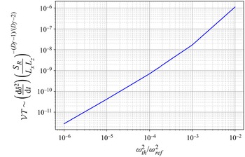
 $D_{f2}$ obtained in the previous section for different enstrophy thresholds, and plot in figure 19 the turbulent viscosity
 $\nu _T$ given by (5.6) with
 $c$ set to a constant independent of
 $\omega _{th}^{2}/\omega _{ref}^{2}$, and
 $\delta ({{\rm d} \delta }/{{\rm d}t}) = \tfrac {1}{2} ({{\rm d} \delta ^{2}}/{{\rm d}t})$ given by the DNS. The result shows that
 $\nu _{T}$ with
 $c={\rm const.}$ is a monotonically increasing function of
 $\omega _{th}^{2}/\omega _{ref}^{2}$, as required for our improved model to be physically viable. This means that
 $\eta _{T}=\nu _{T}/v_{n}$ is also a monotonically increasing function of
 $\omega _{th}^{2}/\omega _{ref}^{2}$ because (3.2) implies that
 $v_n$ is a decreasing function of
 $\omega _{th}^{2}/\omega _{ref}^{2}$. However, the result in figure 19 also suggests that
 $\nu _{T}$ and
 $\eta _T$ tend to
 $0$ as
 $\omega _{th}^{2}/\omega _{ref}^{2}$ decreases towards
 $0$, whereas
 $\nu _T$ should be tending towards the kinematic viscosity
 $\nu$ in that limit. In the next paragraph, we demonstrate how the model's dimensionless coefficient
 $c (Re_{G},\omega _{th}^{2}/\omega _{ref}^{2})$ can ensure that
 $\nu _T$ tends to
 $\nu$ as
 $\omega _{th}^{2}/\omega _{ref}^{2} \to 0$, i.e. as we move towards the outer edge of the TNTI.
The turbulent viscosity  $\nu _{T}$ given by (5.6) with
 $a/c = 1$ and
 $b=1$ as a function of normalised enstrophy threshold.

We model  $c$ as being a constant independent of both
 $Re_G$ and
 $\omega _{th}^{2}/\omega _{ref}^{2}$ for most enstrophy thresholds within the TNTI except the smallest ones, where we approximate it as
 $c (Re_{G},\omega _{th}^{2}/\omega _{ref}^{2}) \approx Re_{G}\,\tilde {c} (\omega _{th}^{2}/\omega _{ref}^{2})$, with
 $\tilde {c}$ being a function of
 $\omega _{th}^{2}/\omega _{ref}^{2}$ but not of
 $Re_G$. Given that
 $\delta ({{\rm d} \delta }/{{\rm d}t}) = ({A}/{2}) U_{J}H_{J}$ (from (2.20)), we can write
 $2a ({\delta }/{c}) ({{\rm d} \delta }/{{\rm d}t}) \approx Aa ({\nu }/{\tilde {c}})$ as
 $\omega _{th}^{2}/\omega _{ref}^{2}\to 0$, i.e.
 \begin{equation} \nu_{T} \sim Aa\,\frac{\nu}{\tilde{c}} \left( \frac{S}{bL_x L_z} \right)^{-(D_{f2}-1)/(D_{f2}-2)} \end{equation}
in that limit. For  $\nu _{T}$ to tend to
 $\nu$ as
 $\omega _{th}^{2}/\omega _{ref}^{2}\to 0$,
 $\tilde {c}$ must tend to
 $0$ at the same rate as
 $({S}/{bL_x L_z} )^{-(D_{f2}-1)/(D_{f2}-2)}$, i.e.
 \begin{equation} \ln \tilde{c} \approx{-}\frac{D_{f2}-1}{D_{f2}-2} \ln \left(\frac{S}{bL_{x}L_{z}}\right) + {\rm const.} \end{equation}
as  $\omega _{th}^{2}/\omega _{ref}^{2}\to 0$. It is not the goal of this paper's final part to determine the functions
 $\nu _{T}(Re_{G}, \omega _{th}^{2}/\omega _{ref}^{2})$ and
 $c(Re_{G}, \omega _{th}^{2}/\omega _{ref}^{2})$ in the improved model for
 $v_n$ based on (5.4), (5.5) and (3.2); the goal here is simply to demonstrate on the basis of our DNS and simple asymptotic arguments that such a model can be physically viable. The example of a choice of
 $c(Re_{G}, \omega _{th}^{2}/\omega _{ref}^{2})$ that we made at the start of this paragraph ensures that
 $\nu _T$ remains a monotonically increasing function of
 $\omega _{th}^{2}/\omega _{ref}^{2}$ while at the same time tending to
 $\nu$ as
 $\omega _{th}^{2}/\omega _{ref}^{2}$ tends to
 $0$. We now work out the consequences of this choice for
 $\eta _T$ and
 $v_n$.
The formulae for  $v_n$ and
 $\eta _{T}$ that can be derived readily from our improved model are
 \begin{equation} v_{n}/u_{\eta}\sim \left(\frac{c^{(D_{f2}-2)}}{b}\right)^{{1}/({D_{f2}-1})} \left(Aa\right)^{{1}/({D_{f2}-1})} Re_{G}^{-({D_{f2}-2})/({D_{f2}-1})+{1}/{4}}\left(\nu_{T}/\nu \right)^{({D_{f2}-2})/({D_{f2}-1})} \end{equation}
and
 \begin{align} \eta_{T}/\eta &\sim
\left(\frac{c^{(D_{f2}-2)}}{b}\right)^{-1/({D_{f2}-1})}
(Aa)^{-{1}/({D_{f2}-1})}
Re_{G}^{({D_{f2}-2})/({D_{f2}-1})
-{1}/{4}}\nonumber\\&\quad \times (\nu_{T}/\nu)^{-({D_{f2}-2})/({D_{f2}-1})}(\nu_{T}/\nu).
\end{align}
Note that the original model of § 2 leads to  $v_{n}/u_{\eta }\sim (Aa)^{{1}/({D_{f2}-1})} Re_{G}^{-({D_{f}-2})/({D_{f}-1})+{1}/{4}}$ and
 $\eta _{I}/\eta \sim (Aa)^{-{1}/({D_{f2}-1})} Re_{G}^{({D_{f}-2})/({D_{f}-1}) -{1}/{4}}$ without the extra powers of
 $c^{D_{f2}-2}/b$ and
 $\nu _{T}/\nu$ in (5.9) and (5.10).
Without these extra powers, the original model predicts the dependence of  $v_n$ on
 $\omega _{th}^{2}/\omega _{ref}^{2}$ very well. In our improved model,
 $(\nu _{T}/\nu )^{({D_{f2}-2})/({D_{f2}-1})}$ is an increasing function of enstrophy threshold because
 $\nu _{T}/\nu$ is increasing and because the exponent
 $({D_{f2}-2})/({D_{f2}-1})$ is also increasing given that
 $D_{f2}$ is an increasing function of
 $\omega _{th}^{2}/\omega _{ref}^{2}$ as observed in our DNS. Our improved model is therefore capable of maintaining the original model's good prediction for
 $v_n$ if the increasing dependence of
 $(\nu _{T}/\nu )^{({D_{f2}-2})/({D_{f2}-1})}$ on
 $\omega _{th}^{2}/\omega _{ref}^{2}$ compensates the decreasing dependence of
 $(c^{D_{f2}-2}/b)^{1/(D_{f2}-1)}$ on
 $\omega _{th}^{2}/\omega _{ref}^{2}$. Indeed,
 $c^{D_{f2}-2}/b$ is not equal to 1, and
 $(c^{D_{f2}-2}/b)^{1/(D_{f2}-1)}$ is a decreasing function of enstrophy threshold, in agreement with our DNS observation in figure 17(c). The entire point of our improved model has been to show that by introducing the generalised Corrsin length and the turbulent viscosity
 $\nu _T$, it is possible to correct our original model's wrong assumption
 $c^{D_{f2}-2}/b =1$ without compromising its correct predictions.
We now show that the choice of  $c$ that we made for
 $\nu _T$ to tend to
 $\nu$ as
 $\omega _{th}^{2}/\omega _{ref}^{2} \to 0$ also ensures that the generalised Corrsin length
 $\eta _T$ tends to a finite value in that limit. As we move within the TNTI from high to low iso-enstrophy levels – i.e. as we take the limit of
 $\omega _{th}^{2}/\omega _{ref}^{2}$ decreasing towards very small values close to 0 and we approach the outer edge of the viscous superlayer –
 $D_{f2}$ tends towards values close to
 $2$, and
 $\nu _{T}$ tends to
 $\nu$, assuming
 $c (Re_{G},\omega _{th}^{2}/\omega _{ref}^{2}) \approx Re_{G}\,\tilde {c} (\omega _{th}^{2}/\omega _{ref}^{2})$ in that limit. We are therefore left with
 \begin{equation} v_{n}/u_{\eta}\sim \tilde{c}^{({D_{f2}-2})/({D_{f2}-1})} Re_{G}^{{1}/{4}} \end{equation}
and
 \begin{equation} \eta_{T}/\eta \sim \tilde{c}^{-({D_{f2}-2})/({D_{f2}-1})} Re_{G}^{-{1}/{4}} \end{equation}
as we approach the outer edge of the viscous superlayer (we have omitted the unimportant factor  $Aa/b$). Finally, (5.8) implies
 $\tilde {c}^{({D_{f2}-2})/({D_{f2}-1})} \sim L_{x}L_{y}/S$, and therefore our generalised model's predictions for the viscous superlayer where
 $D_{f2}$ is very close to
 $2$ and
 $\omega _{th}^{2}/\omega _{ref}^{2}$ is extremely small are
 \begin{equation} v_{n}/u_{\eta}\sim \frac{L_{x}L_{z}}{S_{\nu}}\,Re_{G}^{{1}/{4}} \end{equation}
and
 \begin{equation} \eta_{T}/\eta \sim \frac{S_{\nu}}{L_{x}L_{z}}\,Re_{G}^{-{1}/{4}}, \end{equation}
where  $S_{\nu }$ is the finite surface area of the effectively smooth viscous superlayer of the TNTI. Our generalised model with
 $c (Re_{G},\omega _{th}^{2}/\omega _{ref}^{2}) \approx Re_{G}\, \tilde {c} (\omega _{th}^{2}/\omega _{ref}^{2})$, and (5.8) at the very smallest enstrophy levels and
 $c=1$ above those enstrophy levels, implies that
 $\eta _{T}$ is a monotonically increasing function of
 $\omega _{th}^{2}/\omega _{ref}^{2}$ with a finite value different from
 $\eta$ by a factor
 $Re_{G}^{-1/4}$ at the very smallest enstrophy thresholds. The exponent
 $1/4$ being small, this prediction is not easy to check as it requires numerical oscillation-free calculations at low enstrophy thresholds for many highly resolved DNS of temporally developing turbulent jets over a wide range of Reynolds numbers
 $Re_G$. (See Appendix B for some details about higher Reynolds number simulations and the importance of spatial resolution.) This is at, and perhaps even beyond, the very limit of the most powerful current computational capabilities and therefore beyond the present paper's scope. Such a computational check would also require a computable definition or surrogate for
 $\eta _T$, which we make a first attempt to give in the next couple of paragraphs. Before doing so, however, we point out that Silva et al. (Reference Silva, Zecchetto and da Silva2018) argued that the viscous superlayer thickness scales with the Kolmogorov length if
 $Re_{\lambda }$ is larger than approximately
 $200$, and that the TNTI layer's characteristic sizes may have different scalings at smaller values of
 $Re_{\lambda }$ depending on presence or absence of mean shear (see da Silva & Taveira (Reference da Silva and Taveira2010) and references therein). It must be stressed that the definition of the viscous superlayer used by Silva et al. (Reference Silva, Zecchetto and da Silva2018) does not necessarily include some low iso-enstrophy surfaces with fractal dimensions clearly larger than
 $2$ (see the discussion around figure 11 in § 5.4) and, more importantly, is not local in enstrophy threshold (i.e. it does not depend on the local position within the TNTI) and is therefore different from
 $\eta _{T}$, which is local in enstrophy threshold. The scaling (5.14) does not necessarily contradict the scalings in Silva et al. (Reference Silva, Zecchetto and da Silva2018) as they concern different quantities.
We close this section with an interpretation of the generalised Corrsin length  $\eta _T$. As
 $\eta _T$ is local in terms of iso-enstrophy levels within the TNTI, and as it expresses some kind of thickness of iso-enstrophy surfaces, it appears natural to compare it with some average enstrophy length scale on the TNTI. To this end, we use enstrophy profiles conditioned on the interface location similar to Bisset, Hunt & Rogers (Reference Bisset, Hunt and Rogers2002). We define a local coordinate system with local coordinate
 $y_I$ chosen along the local unit normal
 ${\boldsymbol n} = -({\boldsymbol {\nabla } \omega ^2}/{|\boldsymbol {\nabla } \omega ^2|})$, which is pointing towards the non-turbulent region. The origin
 $y_I = 0$ of this local coordinate system is placed at a given location within the TNTI, for example on the isosurface defined by
 $\omega ^2_{th}/ \omega _{ref}^2 = 10^{-6}$, located at the very edge of the TNTI neighbouring the non-turbulent region. In this way, positive values of
 $y_I$ correspond to the very edge of the viscous superlayer and the non-turbulent region, whereas negative values of
 $y_I$ are within the TNTI and the turbulent region. Given such local coordinate systems on the TNTI, we calculate averages of any quantity
 $\phi$ at a given
 $y_I$ over all locations on the TNTI where the local
 $y_I$ axis does not cross the TNTI more than once in the range
 $y_I\in [-27\eta, +27\eta ]$. We use the notation
 $\phi _{I}$ to denote these average quantities, averaged conditionally on the specified isosurface location.
Figure 20 shows the vorticity magnitude,  $\vert\omega\vert_I$, and the enstrophy profile,
 $\omega_I^2$, averaged conditionally on the distance from the enstrophy isosurface
 $\omega _{th}^{2}/\omega _{ref}^{2}=10^{-6}$; the profiles are normalised by the average values of the respective quantities at the centreplane. The drastic change of both vorticity and enstrophy values in a very short distance is visible, as shown previously in studies using similar methods, e.g. Nagata et al. (Reference Nagata, Watanabe and Nagata2018), Silva et al. (Reference Silva, Zecchetto and da Silva2018) and Watanabe, da Silva & Nagata (Reference Watanabe, da Silva and Nagata2019).
Vorticity magnitude and enstrophy values averaged conditionally on the distance from the iso-enstrophy surface defined by  $\omega _{th}^{2}/\omega _{ref}^{2}=10^{-6}$ for the simulation PJ1.

We define the local length  $\eta _{\omega } \equiv (({{\rm d}\omega ^2_{I}}/{{\rm d}y_{I}}) ({1}/{\omega ^2_{I}}))^{-1}$. In figure 21(a), we plot
 $\eta _{\omega }/\eta$ versus
 $\omega ^{2}_{I}/\omega _{ref}^{2}$. In agreement with
 $\eta _{T}$,
 $\eta _{\omega }$ is an increasing function of enstrophy,
 $\omega ^{2}_{I}/\omega _{ref}^{2}$ in this case: iso-enstrophy surfaces get further away from each other on average as
 $\omega ^{2}_{I}/\omega _{ref}^{2}$ increases within the TNTI. At the very smallest enstrophy thresholds,
 $\eta _{\omega }$ appears to tend to a finite value that is significantly smaller than
 $\eta$, which is also in agreement with
 $\eta _{T}$ at high enough
 $Re_G$ (see (5.14)).
(a) Plot of  $\eta _{\omega }/\eta$ versus
 $\omega ^{2}_{I}/\omega _{ref}^{2}$ for
 $t/T_{ref}=50$, PJ1 simulation. This plot is typical of all times
 $t/T_{ref}$ between
 $30$ and
 $100$. (b) Profile of
 $\eta _{\omega }$ along
 $y_{I}/\eta$, with
 $y_{I}=0$ at
 $\omega ^2_{th}/ \omega _{ref}^2 = 10^{-6}$.

We also plot  $\eta _{\omega }/\eta$ versus
 $y_{I}/\eta$ in figure 21(b), where
 $y_{I}=0$ corresponds to the iso-enstrophy surface
 $\omega ^2_{th}/ \omega _{ref}^2 = 10^{-6}$. We see that the profile of
 $\eta _{\omega }$ along
 $y_I$ is decreasing exponentially with increasing
 $y_I$. The linear region ends near
 $y_I/\eta \approx -2.5$. This is due to some points where the normal enstrophy profiles do not decrease monotonically to zero when going towards the non-turbulent region, even though the local enstrophy values always remain lower than the threshold value.
6. Conclusion
To determine the mean flow profile evolution, we have applied to the temporally developing turbulent planar jet the approach typically applied to spatially developing free turbulent shear flows. This approach is based on self-similarity and on mass, momentum and turbulent kinetic energy balance equations (Townsend Reference Townsend1976; George Reference George1989; Cafiero & Vassilicos Reference Cafiero and Vassilicos2019). The turbulent kinetic energy equation involves the turbulence dissipation rate, and one needs to specify the turbulence dissipation rate's scalings in order to close the problem. The mechanism for turbulence dissipation being the turbulence cascade, different types of turbulence cascade (e.g. equilibrium, non-equilibrium, balanced non-equilibrium; see Dairay et al. Reference Dairay, Obligado and Vassilicos2015; Vassilicos Reference Vassilicos2015; Goto & Vassilicos Reference Goto and Vassilicos2016; Cafiero & Vassilicos Reference Cafiero and Vassilicos2019) in the presence of different types of large-scale coherent structures can lead to different turbulence dissipation scalings (Goto & Vassilicos Reference Goto and Vassilicos2016; Ortiz-Tarin et al. Reference Ortiz-Tarin, Nidhan and Sarkar2021). In turn, different dissipation scalings lead to different self-similar mean flow profile evolutions, as found already in various spatially developing turbulent flows (e.g. Dairay et al. Reference Dairay, Obligado and Vassilicos2015; Vassilicos Reference Vassilicos2015; Cafiero & Vassilicos Reference Cafiero and Vassilicos2019; Ortiz-Tarin et al. Reference Ortiz-Tarin, Nidhan and Sarkar2021), and to different TNTI mean propagation speeds, as demonstrated by Cafiero & Vassilicos (Reference Cafiero and Vassilicos2020) for the spatially developing turbulent planar jet.
The temporally developing self-similar turbulent planar jet is exceptional because the scalings of its mean flow profile evolution do not depend on the scalings of the turbulence dissipation rate. Whatever the exponent  $m$ in (2.18), the scalings of the centreline mean flow velocity
 $u_0$ and jet width
 $\delta$ are given by (2.19) and (2.20). The reason why the temporally developing self-similar jet is fundamentally different from its spatially developing counterpart is that it conserves volume flux and has identically zero cross-stream mean flow velocity, whereas spatially developing turbulent planar jets do not conserve volume flux and do not have identically zero cross-stream mean flow velocity. As a result, in the case of the temporally developing self-similar turbulent planar jet, the jet width
 $\delta$, the Kolmogorov length
 $\eta$ and the Taylor length
 $\lambda$ all grow as the square root of time, and the centreline velocity
 $u_0$, the Kolmogorov velocity
 $u_{\eta }$ and the TNTI mean propagation speed all decay as the inverse square root of time, irrespective of turbulence dissipation scaling. The Taylor length Reynolds number remains constant in time. All these theoretical predictions and the assumptions on which they are based have been verified by our DNS of a temporally evolving turbulent planar jet. Note that the volume flux that is conserved in our flow is not conserved in many other flows with a TNTI besides spatially developing jets such as wakes (e.g. Watanabe et al. Reference Watanabe, Riley, De Bruyn Kops, Diamessis and Zhou2016), boundary layers (e.g. Borrell & Jimenez Reference Borrell and Jimenez2016) and mixing layers (e.g. Attili, Cristancho & Bisetti Reference Attili, Cristancho and Bisetti2014; Balamurugan et al. Reference Balamurugan, Rodda, Philip and Mandal2020). One should therefore be very careful if attempting to extend the applicability of this paper's results to other turbulent flows with a TNTI.
The prediction for the TNTI mean propagation speed has been made on the basis of: (i) a proportionality between the turbulent jet volume and the jet width growth rates that has been verified by our DNS; (ii) an assumption that the TNTI is fractal with a well-defined fractal dimension; (iii) an assumption that the smallest geometrical scale on the TNTI scales with the Corrsin length that characterises generation of vorticity by viscous diffusion; and (iv) a particular way to blend assumptions (ii) and (iii) together, (3.5). The geometrical picture of the TNTI returned by our DNS has turned out to be more involved than assumptions (ii), (iii) and (iv), which make no reference to the TNTI's inner structure. Even so, the prediction that the TNTI mean propagation speed evolves as the inverse square root of time has been validated by our DNS.
The TNTI has an inner structure over a wide range of closely spatially packed iso-enstrophy surfaces, and it turns out that different iso-enstrophy surfaces have different fractal dimensions. These fractal dimensions vary from approximately  $7/3$ at the innermost iso-enstrophy surface on the fully turbulent side of the TNTI, to close to
 $2$ at the outermost iso-enstrophy surface on the non-turbulent flow side of the TNTI. However, the
 $7/3$ value, which, according to the theory based on assumptions (i), (ii) and (iii), corresponds to a TNTI mean propagation speed that scales with the Kolmogorov velocity
 $u_{\eta }$, is not well-defined in the sense that it is a fit through a range of scales where the fractal dimension is not scale-independent as it should be. Lower fractal dimension values between approximately
 $2.2$ and under
 $2.1$ are found for iso-enstrophy surfaces with lower enstrophy values, i.e. towards the TNTI's outer side. These lower fractal dimensions are well-defined in a range of scales bounded by
 $\lambda$ from below and
 $\delta$ from above. However, the smallest geometrical scales on these iso-enstrophy surfaces are close to
 $\eta$, and the scales between
 $\lambda$ and
 $\eta$ contribute significantly to the surface areas of the iso-enstrophy surfaces even though these scales are not characterised by a well-defined fractal dimension. The formula for the TNTI mean propagation speed
 $v_n$ obtained from assumptions (i), (ii) and (iii) captures its time dependence because the time dependence is the same for all iso-enstrophy surfaces. Perhaps remarkably, it also captures the iso-enstrophy dependence of
 $v_n$ via the iso-enstrophy dependence of the fractal dimension. However, the DNS invalidate (3.5), on which the formula for
 $v_n$ is partly based, and support a form such as (5.5) instead.
Having found that different iso-enstrophy surfaces within the TNTI have different sufficiently well-defined fractal dimensions over a range of scales bounded from below by  $\lambda$, and that length scales below
 $\lambda$ on these surfaces do also contribute significantly to their surface area, it is not possible to argue sweepingly that the Corrsin length
 $\eta _{I}$ is the smallest length scale on the fractal/fractal-like/multiscale TNTI. Aiming to keep the model's correct predictions while at the same time abandoning wrong premise (iv), we nevertheless keep the main structure of our model by keeping assumptions (i) and (ii), and modifying (iii) and (iv). For this, we introduce a generalised Corrsin length defined on the basis of an iso-enstrophy surface-dependent turbulent viscosity
 $\nu _T$ that tends to the fluid's kinematic viscosity
 $\nu$ as the iso-enstrophy level tends to near-vanishing values at the viscous superlayer, but is independent of
 $\nu$ at higher iso-enstrophy levels. We demonstrate the physical viability of such a model, but leave for future investigation the detailed relation between
 $\nu _T$ and the enstrophy production processes, which vary from being viscosity dominated at the outer edge of the TNTI (viscous superlayer) to being controlled by vortex stretching further in. We do, however, show with our DNS that the generalised Corrsin length depends on iso-enstrophy levels similarly to the length scale
 $\eta _{\omega }$ defined by the local enstrophy gradients within the TNTI: in particular,
 $\eta _{\omega }$ is smaller than
 $\eta$ at the outer edge of the TNTI, larger than
 $\eta$ at the inner edge of the TNTI, and monotonically increasing in between. Even if incomplete at this stage, our revised model predicts that the mean propagation speed at the outer edge of the viscous superlayer is proportional to the Kolmogorov velocity multiplied by the power
 $1/4$ of the global Reynolds number. We stress that this prediction is specific to temporally developing self-similar turbulent planar jets, which are very idiosyncratic flows, and that it should not necessarily be extended to spatially developing free turbulent shear flows. Current computational capabilities at our disposal are insufficient for the wide range of global Reynolds number required to verify this prediction.
Acknowledgements
This work was supported by the European Community, the French Ministry for Higher Education and Research, and the Hauts de France Regional Council in connection with CNRS Research Foundation on Ground Transport and Mobility as part of the ELSAT2020 project. This work was granted access to the HPC resources of IDRIS under the allocation 2021-021741 made by GENCI (Grand Equipement National de Calcul Intensif).
Funding
This work was supported by J.C.V.'s Chair of Excellence CoPreFlo, funded by I-SITE-ULNE (grant no. R-TALENT-19-001-VASSILICOS), MEL (grant no. CONVENTION_219_ESR_06) and Region Hauts de France (grant no. 20003862).
Declaration of interests
The authors report no conflict of interest.
Appendix A
We are interested in fine details of the TNTI layer that is located at the boundary between the turbulent and non-turbulent regions of the flow. At the outer edge of the TNTI, the enstrophy value decays quickly to zero. We investigate how quantities such as  $D_f$ and
 $v_n$ vary with enstrophy threshold value. A wide range of enstrophy threshold values is considered, all located in the plateaus shown in figure 7, and the lowest that we consider here reach
 $\omega ^2_{th}/\omega ^2_{ref}=10^{-6}$. In order to obtain relevant TNTI statistics at such very low enstrophy levels, the DNS solution must be smooth and free of oscillations. When using a classical
 $2/3$ truncation de-aliasing method for the simulations with the pseudo-spectral code, we observe numerical oscillations at these low enstrophy values, which makes it impossible to investigate this very low enstrophy part of the TNTI layer. The limiting effect of these oscillations has been mentioned in the study of Krug et al. (Reference Krug, Chung, Philip and Marusic2017). The solution is to use a modified de-aliasing method as explained in § 4. A similar procedure is applied in Krug et al. (Reference Krug, Chung, Philip and Marusic2017), with their choice of a
 $p$th-order Fourier exponential filter for the de-aliasing. Our method, which has no effect on the modes unaffected by the aliasing, is able to suppress the oscillations within the useful range of enstrophy. As we are dealing with a very sharp interface and need to reduce our enstrophy thresholds to extremely low values, the numerical oscillations naturally become observable at some point, particularly without a special treatment being employed. This is due to the fact that the spectral method does not underestimate the derivatives and does not smooth out sharp gradients, as is the case with finite difference methods, for example.
In order to demonstrate how the classical sharp de-aliasing leads to some oscillations and the effectiveness of our modified de-aliasing method, we compare two simulations starting from identical initial conditions, solved by the same pseudo-spectral solver. The first simulation was performed with the classical sharp de-aliasing method that truncates the solution at all wavenumbers with modulus larger than  $2/3 k_{max}=N/3$, and the second simulation uses our modified de-aliasing method. As can be observed in figure 1(b), the minimum value of the mean Kolmogorov scale
 $\eta$ on the centreline appears just after the transition, and we therefore compare the solutions of the two simulations at
 $t/T_{ref} = 26$ where the grid resolution is most problematic. We also consider the simulation PJ5, which has the highest
 $Re_\lambda$ peak. The two simulations are initialised with the same initial conditions.
Figures 22(a,b) show the enstrophy in a normal streamwise plane for the two simulations at  $t/T_{ref} = 26$. Figure 22(a) corresponds to the simulation with the modified de-aliasing, and figure 22(b) is the case where the classical
 $2/3$ truncation method is used. Oscillations are clearly visible in the case of classical de-aliasing, even for normalised enstrophy levels higher than
 $10^{-3}$, whereas the solution is smooth for all investigated enstrophy levels with our modified de-aliasing method.
Enstrophy fields in a normal streamwise plane for two identical simulations PJ5: (a,c) with modified de-aliasing (used in the present study), and (b,d) with classical  $2/3$ truncation, for (a,b)
 $t/T_{ref} = 26$, and (c,d)
 $t/T_{ref} = 50$. The same colours are used for
 $\omega ^2/\omega ^2_{ref}$ isocontours as in figure 8, where magenta and cyan correspond to
 $\omega ^2/\omega ^2_{ref}=10^{-3}$ and
 $10^{-6}$, respectively.

It should be noted that the oscillations are visible at fairly high enstrophy thresholds at this instant, and that these oscillations gradually reduce with time, but do not disappear at the targeted enstrophy thresholds  $\omega ^2_{th}/\omega ^2_{ref} > 10^{-6}$ for
 $t/T_{ref}>30$ with the classical
 $2/3$ truncation method. In figures 22(c,d), enstrophy contours are given for
 $t/T_{ref} > 50$, which is in the time range for which we investigate the TNTI characteristics. Although some enstrophy isocontours appear to be smooth, local regions where the oscillations are present may introduce significant problems. For example, the computation of
 $D_f$ would be affected by these oscillations, as the isosurface becomes more volume filling in the presence of these numerical artefacts.
To quantify the energy content of these oscillations, the energy and dissipation spectra on the centreplane are compared for the two simulations in figure 23. The spectra look identical for both cases, apart from the small peak at the very end of the resolved wavenumbers that is present for the classical  $2/3$ truncation method. This shows how difficult it is to assess the smoothness of the irrotational region and the external part of the TNTI from energy and dissipation spectra.
(a) Energy and (b) dissipation spectra at the centreplane of two identical simulations in terms of flow parameters and initial conditions, one with modified de-aliasing, and the other with the classical  $2/3$ truncation method. Results are from the simulation PJ5 at
 $t/T_{ref} = 26$.

In figure 24, the jet volume as a function of the enstrophy threshold (similar to figure 7) is plotted at  $t/T_{ref} = 26$ for the two simulations with classical and modified de-aliasing methods. A clear extension of the plateau towards lower values of
 $\omega ^2_{th}/\omega ^2_{ref}$ is seen when the modified de-aliasing method is used. Meanwhile, the high threshold regions remain unaffected by the modification, showing that the de-aliasing method works as planned. It suppresses the weak oscillations at the outer regions of the TNTI, but the evolution of the turbulent region is similar in both cases.
The jet volume defined as  $\omega ^2 > \omega ^2_{th}$ for the two simulations PJ5 at
 $t/T_{ref} = 26$ with modified de-aliasing (blue) and classical
 $2/3$ truncation (orange).

Appendix B
In § 5.6, the relation (5.10) for  $\eta _T/\eta$ has been simplified for the iso-enstrophy surfaces at the very outer edge of the viscous superlayer by using
 $D_{f2} \approx 2$ due to the fact that
 $D_{f2} \rightarrow 2$ when
 $\omega ^2_{th}/\omega ^2_{ref} \rightarrow 0$. This simplification leads to (5.14), where a scaling due to the global Reynolds number
 $Re_G$ is present with power
 $-1/4$.
In an attempt to obtain a data set spanning a range of Reynolds numbers to investigate this scaling, additional simulations have been conducted with  $Re_G=6400$ and
 $Re_G=9600$, which will be referred as PJ-Re6400 and PJ-Re9600, respectively. The initial conditions and the solver properties remain the same as described in § 4. The computational grid also remains the same as the PJ1–PJ5 simulations, due to the computational constraints.
With the increase of  $Re_G$, the Reynolds number based on Taylor length scale
 $Re_\lambda$ at the centreplane of the jet becomes
 $Re_\lambda \approx 70$ and
 $Re_\lambda \approx 80$ for the simulations PJ-Re6400 and PJ-Re9600, compared to
 $Re_\lambda \approx 50$ for the PJ1 simulation (labelled as
 $Re_G=3200$), which can be seen in figure 25(a). Figure 25(b) shows the time evolution of the spatial resolution normalised by the Kolmogorov scale at the centreplane after the transition to the fully turbulent regime.
Plots of (a)  $Re_\lambda$ and (b) resolution
 ${{\rm d} y}/\eta$ at the centreplane of the planar jet for
 $Re_G=3200$ (PJ1 simulation),
 $Re_G=6400$ and
 $Re_G=9600$.

Following Appendix A, we focus on time  $t/T_{ref} = 50$ as this time is in the middle of the investigated time range in this study to analyse the state of the data. Figure 26 shows the enstrophy contours at the cut-section of the PJ-Re6400 simulation, along with the enstrophy isosurfaces marked at the TNTI.
Enstrophy contour field at a cut-section of the simulation PJ-Re6400 at  $t/T_{ref} = 50$, with iso-enstrophy contours from
 $\omega ^2_{th}/\omega ^2_{ref} = 10^{-6}$ to
 $10^{-3}$ shown at the TNTI.

It is observed that numerical oscillations are present in the enstrophy isosurfaces due to the reduction of the resolution of the simulations. The oscillations are present even at the isosurfaces of enstrophy thresholds up to  $\omega ^2_{th}/\omega ^2_{ref} = 10^{-4}$. Under these conditions, the application of the box-counting algorithm is not possible for
 $\omega ^2_{th}/\omega ^2_{ref} \lesssim 10^{-3}$, while (5.14) is obtained for the very outer enstrophy isosurfaces that have
 $D_{f2} \approx 2$.