1 Introduction
The Richtmyer–Meshkov instability (RMI) occurs when a moving shock wave passes through a gas interface separating fluids with different densities. RMI can be considered the Rayleigh–Taylor instability (RTI) under impulsive acceleration. Richtmyer (Reference Richtmyer1960) first theoretically investigated RMI from the viewpoint of linear stability analysis, and Meshkov (Reference Meshkov1969) provided experimental confirmation.
The RMI problem occurs widely in nature and engineering practice. This problem naturally exists in the situation of shock–magnetosphere interactions and supernova explosions. Its practical applications include but are not limited to the mixing enhancement of supersonic flow, the interaction of a shock wave and a premixed or non-premixed flame and inertial confinement fusion. Academically, the RMI problem is of fundamental significance in the interaction of a shock wave and compressible turbulence. The interaction of a shock and a spherical or cylindrical gas interface is known as shock–bubble interaction (SBI), which is a special case of the RMI problem. It occurs in supersonic combustion systems, shock propagation through foams and bubbly liquids, the fragmentation of gallstones or kidney stones by shock waves and many other situations. Comprehensive reviews of the occurrence and applications of the RMI and SBI problem have been made by Holmes et al. (Reference Holmes, Dimonte, Fryxell, Gittings, Grove, Schneider, Sharp, Velikovich, Weaver and Zhang1999), Brouillette (Reference Brouillette2002), Zhou (Reference Zhou2017a,Reference Zhoub) and Ranjan, Oakley & Bonazza (Reference Ranjan, Oakley and Bonazza2011).
During the shock and gas interface interaction, vorticity deposition on the gas interface occurs. This phenomenon is mainly due to the misalignment of the pressure gradient across the shock and the density gradient across the interface, namely, the baroclinicity of the flow. In RMI, the initial deposition and further evolution of the vorticity significantly affect the RMI process in many different aspects (Zhou Reference Zhou2017a), including RMI-induced mixing (Zabusky Reference Zabusky1999), pressure perturbations across the interface (Fraley Reference Fraley1986), rolling up of the interface into mushroom-like spikes (Morgan et al. Reference Morgan, Aure, Stockero, Greenough, Cabot, Likhachev and Jacobs2012) and growth of the primary and secondary instabilities (Reinaud, Joly & Chassaing Reference Reinaud, Joly and Chassaing2000; Peng, Zabusky & Zhang Reference Peng, Zabusky and Zhang2003). Thus, the vorticity deposition and evolution are crucial mechanisms that define the flow evolution. Considering these mechanisms leads to a deep and broad physical understanding of the RMI problem (Hawley & Zabusky Reference Hawley and Zabusky1989). Zabusky (Reference Zabusky1999) reviewed the investigations considering the vortex paradigm in the RTI and RMI problems.
1.1 Circulation deposition and predicting models
Circulation deposition is a dominant fluid dynamical process and a global quantification of the vorticity generation in the early-time RMI process (Zabusky Reference Zabusky1999). Considerable attention has been paid to the theoretical prediction of the initial circulation deposition on the gas interface during the interaction (Rudinger & Somers Reference Rudinger and Somers1960; Picone et al. Reference Picone, Oran, Boris and Young1984; Picone & Boris Reference Picone and Boris1988; Yang, Kubota & Zukoski Reference Yang, Kubota and Zukoski1991; Yang et al. Reference Yang, Chern, Zabusky, Samtaney and Hawley1992; Samtaney & Zabusky Reference Samtaney and Zabusky1993, Reference Samtaney and Zabusky1994; Yang, Kubota & Zukoski Reference Yang, Kubota and Zukoski1994; Samtaney & Meiron Reference Samtaney and Meiron1997; Samtaney, Ray & Zabusky Reference Samtaney, Ray and Zabusky1998; Niederhaus et al. Reference Niederhaus, Greenough, Oakley, Ranjan, Anderson and Bonazza2008).
The most general and commonly used predicting model of circulation deposition is the Samtany–Zabusky (SZ) model. Yang et al. (Reference Yang, Chern, Zabusky, Samtaney and Hawley1992) first quantitatively studied the vorticity deposition and evolution in the RMI problem with a fast/slow or slow/fast gas interface. The results were compared with shock tube experiments and shock polar analysis, and good agreement is obtained. Then, the circulation model was elaborately derived and validated by Samtaney & Zabusky (Reference Samtaney and Zabusky1993, Reference Samtaney and Zabusky1994) and named after them. The SZ model, which is based on the shock polar analysis (Henderson Reference Henderson1966), theoretically solves the velocity field in the vicinity of the three-shock intersection. Then, the circulation deposited per unit length of the gas interface is directly obtained by integrating the velocity along a contour on both sides of the shocked interface and parallel to it. They provided the scaling law of the circulation with basic parameters of the initial conditions (incident Mach number, initial density ratio, local slope of the unshocked interface and specific heat ratio) by utilising the asymptotic analysis. The model is generalised for sinusoidal and circular interfaces and gives satisfactory agreement with the numerical results. Samtaney et al. (Reference Samtaney, Ray and Zabusky1998) generalised the SZ model for the slow/fast interface condition by using Prandtl–Meyer expansion theory for the rarefaction wave. The SZ model was extended to the hypervelocity RMI by Samtaney & Meiron (Reference Samtaney and Meiron1997). The Lighthill–Freeman ideal dissociating gas model is employed instead of the state equation of ideal gas considering the dissociation chemistry under extremely high Mach numbers.
In the SBI case, there are mainly four predicting models of circulation deposition, namely, the Rudinger–Somers (RS) model (Rudinger & Somers Reference Rudinger and Somers1960), Picone–Boris (PB) model (Picone et al. Reference Picone, Oran, Boris and Young1984; Picone & Boris Reference Picone and Boris1988), Yang–Kubota–Zukoski (YKZ) model (Yang et al. Reference Yang, Kubota and Zukoski1991, Reference Yang, Kubota and Zukoski1994) and the one-dimensional (1-D) model (Niederhaus et al. Reference Niederhaus, Greenough, Oakley, Ranjan, Anderson and Bonazza2008). The RS model considers that the SBI consists of an ‘initial accelerating’ step, in which the bubble is accelerated by the shock and a ‘subsequent transforming’ step, in which the bubble is transformed into a vortex pair. The difference in the impulses to the bubble and surrounding gas and the bubble distortion during the interaction are neglected. The transforming step is then modelled as an impulsive motion of an infinite lamina accelerated from the rest. The circulation is obtained by integrating the modelled steady state velocity field of the vortex pair. The PB and YKZ models consider the surface integral of the baroclinic source over the time of passage of the shock through the bubble as the circulation deposited on the bubble interface. They introduce different assumptions and simplifications to perform the integral. In the PB model, the shock wave is modelled as a planar discontinuity without curvature and the difference between the strength of the incident and transmitted shocks is ignored. The YKZ model approximates the effects of density in the flow field by suitably chosen values of density to avoid the difficulty in modelling the complex density field for integrating the baroclinic source. As for the 1-D model, the 1-D gas dynamics is utilised in the modelling of the velocity field on the central line of the bubble. Then, the circulation deposited on half of the bubble is directly acquired by integrating the velocity along the region boundary of the top half-plane.
Now, we further interpret and classify the above-mentioned circulation models, namely, the SZ, RS, PB, YKZ and 1-D models. The integration of the momentum conservation equation for compressible flow without a body force over a closed material curve  $C$ leads to the governing equation of the circulation rate in that region as (1.1), where
 $\unicode[STIX]{x1D6E4}$ is the circulation,
 $\boldsymbol{V}$ is the velocity vector,
 $\unicode[STIX]{x1D70C}$ is the mass density,
 $p$ is the pressure,
 $\unicode[STIX]{x1D749}$ is the viscous stress tensor and
 $\boldsymbol{s}$ is the length path vector. The superposed dot denotes the time derivative,
 $(\text{D}/\text{D}t)$ represents the material derivative and
 $\unicode[STIX]{x1D735}$ represents the gradient operators. Notably, two different sources, namely, the baroclinic source
 $\dot{\unicode[STIX]{x1D6E4}}_{b}$ and the viscous source
 $\dot{\unicode[STIX]{x1D6E4}}_{v}$, contribute to the circulation deposition.
 $$\begin{eqnarray}\dot{\unicode[STIX]{x1D6E4}}=\oint _{C}\frac{\text{D}\boldsymbol{V}}{\text{D}t}\boldsymbol{\cdot }\text{d}\boldsymbol{s}=-\oint _{C}\unicode[STIX]{x1D70C}^{-1}\unicode[STIX]{x1D735}p\boldsymbol{\cdot }\text{d}\boldsymbol{s}+\oint _{C}\unicode[STIX]{x1D70C}^{-1}\unicode[STIX]{x1D735}\boldsymbol{\cdot }\unicode[STIX]{x1D749}\boldsymbol{\cdot }\text{d}\boldsymbol{s}=\dot{\unicode[STIX]{x1D6E4}}_{b}+\dot{\unicode[STIX]{x1D6E4}}_{v}.\end{eqnarray}$$
The above-mentioned five circulation models can be divided into two classes. The first class includes the PB and YKZ models. These models consider the baroclinic source as the only source of the circulation deposition and model the baroclinic source on the basis of different assumptions, which have been briefly introduced in the preceding paragraph. The growth rate of circulation is then estimated to be equal to the baroclinic source. We term this class as the ‘baroclinic class’ and summarise it as (1.2). Green’s theorem is employed, and  $A$ is the surface with
 $C$ as its boundary. The baroclinic class corresponds to (1.1) with the viscous source
 $\dot{\unicode[STIX]{x1D6E4}}_{v}$ being neglected. The density and pressure fields in SBI are difficult to exactly model. Thus, the circulation models of the baroclinic class are limited in some specific SBI cases due to their simplifications and assumptions (Quirk & Karni Reference Quirk and Karni1996; Niederhaus et al. Reference Niederhaus, Greenough, Oakley, Ranjan, Anderson and Bonazza2008).
 $$\begin{eqnarray}\dot{\unicode[STIX]{x1D6E4}}\approx \dot{\unicode[STIX]{x1D6E4}}_{b}=-\oint _{C}\unicode[STIX]{x1D70C}^{-1}\unicode[STIX]{x1D735}p\boldsymbol{\cdot }\text{d}\boldsymbol{s}=\int _{A}\unicode[STIX]{x1D70C}^{-2}(\unicode[STIX]{x1D735}\unicode[STIX]{x1D70C}\times \unicode[STIX]{x1D735}p)\,\text{d}A.\end{eqnarray}$$
The second class includes the RS, SZ and 1-D models. They model the velocity field and use the definition of circulation (line integral of velocity) to predict its value. We term this class as the ‘velocity class’ and summarise it as (1.3), involving the equivalent relation for the circulation rate. The velocity class corresponds to the first relation of (1.1), which is the Kelvin circulation formula (Wu, Ma & Zhou Reference Wu, Ma and Zhou2007). Thus, the velocity class inherently involves the effects of the baroclinicity and viscosity (without distinguishing them) in the circulation deposition. The circulation in the velocity class can be accurately predicted as long as the velocity field is accurately modelled:
 $$\begin{eqnarray}\unicode[STIX]{x1D6E4}=\oint _{C}\boldsymbol{V}\boldsymbol{\cdot }\text{d}\boldsymbol{s}\Leftrightarrow \dot{\unicode[STIX]{x1D6E4}}=\oint _{C}\frac{\text{D}\boldsymbol{V}}{\text{D}t}\boldsymbol{\cdot }\text{d}\boldsymbol{s}.\end{eqnarray}$$
These two classes of circulation model predict the circulation deposition in different approaches, but none of them can predict the contribution of all the sources (baroclinic and viscous) to the total circulation deposition. In the baroclinic class, the baroclinic source is considered the only source, whilst the viscous source is ignored. Although the velocity class can predict the circulation rate that involves the effects of both sources, it cannot quantitatively distinguish the sources of circulation deposition. Where does the circulation in RMI come from exactly? How much do different mechanisms contribute to the circulation deposition? These issues remain unknown. A predicting model for not only the magnitude of circulation deposition but also both sources (especially the viscous source) in it will broaden our physical understanding of the real circulation deposition mechanisms in RMI. This study focuses on this topic.
1.2 Vorticity deposition, evolution and vortex dynamics
Apart from the initial circulation deposition process, some other aspects of the intermediate- and long-term evolution of RMI are investigated in the viewpoint of vorticity deposition, evolution and vortex dynamics. These aspects include the reshocked RMI (Kotelnikov, Ray & Zabusky Reference Kotelnikov, Ray and Zabusky2000), the secondary baroclinic vorticity deposition (Peng et al. Reference Peng, Zabusky and Zhang2003) and the long-term evolution of circulation (Lee, Peng & Zabusky Reference Lee, Peng and Zabusky2006; Li et al. Reference Li, Wang, Yu, Zhang and Liu2019). Kotelnikov et al. (Reference Kotelnikov, Ray and Zabusky2000) investigated the vortex dynamics and interfacial evolution in RMI with the reshocked interface. The numerical simulations were compared with a free falling tank laboratory experiment, and remarkable agreement in large and intermediate scale features was observed. A comparison of the incompressible and compressible simulations was also made, and discrepancies between the results during the reshock process were obtained. Peng et al. (Reference Peng, Zabusky and Zhang2003) revealed the effects of vortex-accelerated secondary baroclinic vorticity deposition on the intermediate and late time flow evolution in the RMI problem. The numerical simulations of the RMI problem were carried out until the late time evolution, and they agreed with the experimental results in the large scale features. The evolution of enstrophy, vorticity skewness, and flatness were also quantified and investigated. Lee et al. (Reference Lee, Peng and Zabusky2006) introduced a new diagnostic formula for the baroclinic source in the form of a line integral, to model the circulation rate of the RMI problem in the intermediate time period. The approximated circulation rate, which required numerical data for the pressure and density at the gas interface, agreed well with the directly obtained circulation rate from the numerical simulations. Li et al. (Reference Li, Wang, Yu, Zhang and Liu2019) modelled the equilibrium stage vorticity field of SBI as a quasi-Gaussian distribution. A model for steady state circulation of SBI is obtained by integrating the vorticity field. This model requires simulated characters, such as maximal vorticity and variance of the Gaussian distribution, of the vorticity field.
The RMI problem with some other forms of the gas interface has been investigated under the vortex paradigm. Zhang, Peng & Zabusky (Reference Zhang, Peng and Zabusky2005) numerically studied the 2-D and 3-D shock-planar heavy curtain interactions. Vortex dynamics, including primary and secondary vorticity deposition and evolution, generation and interaction of vortex projectiles and some turbulent properties were examined and visiometrically quantified. Hejazialhosseini, Rossinelli & Koumoutsakos (Reference Hejazialhosseini, Rossinelli and Koumoutsakos2013) numerically simulated the 3-D SBI problem at low and high incident Mach numbers. The vorticity generation and evolution due to baroclinicity, stretching and dilatation were quantified and compared. An empirical model for the circulation deposition based on the fitted numerical results was provided.
In the above-mentioned investigations, the baroclinic source is considered the only source of importance and the effects of viscosity are neglected in exploring the vorticity deposition and evolution. Wang et al. (Reference Wang, Yu, Chen, Zhang and Liu2018) investigated the scaling vortex breakdown mechanism due to viscous effects in the SBI problem. A dimensionless parameter was introduced to reflect the ratio of the baroclinic and viscous source contributing to the circulation deposition and evolution, which was also claimed as the main mechanism of scaling breakdown. Their investigation involves only the viscous effects after the passing of the shock wave, and the modelling of the baroclinic and viscous source is empirical. The mechanism of viscosity remains unknown in the vorticity depositing process (the interacting process of the shock and the gas interface).
1.3 Overview of the present work
The present work focuses on the circulation deposition during the interaction. The deposited circulation and the contribution of the viscous source are theoretically derived and numerically studied. The contribution of viscosity to the circulation deposition is revealed, that is, the contribution is positive and significant under high Mach number conditions. The gradient of viscosity, which has always been ignored by previous studies about the vorticity deposition and evolution in RMI, plays a crucial role. This study also provides an exciting opportunity to advance our knowledge of shock wave–turbulence interaction, in which the mechanism of vorticity transfer is a fundamental problem (Andreopoulos, Agui & Briassulis Reference Andreopoulos, Agui and Briassulis2000). In addition to the circumstances with shock waves, such as the RMI considered here, the large viscosity gradient naturally and practically exists in many other situations (Govindarajan & Sahu Reference Govindarajan and Sahu2014). The viscosity gradient is supposed to also make a significant contribution to the vorticity evolution in these circumstances.
In § 2, we introduce the substantial method of our theoretical predictions of the circulation deposition process, and it is considered as the single-shock problem. In § 3, the single-shock problem is handled theoretically and is validated by numerical simulations of single shocks. In § 4, we derive the prediction of the incident and transmitted shock strengths based on the asymptotic method. Then, the circulation rate and contribution of viscous source are calculated. Basic features of these are theoretically analysed. In § 5, RMI problems in a large range of initial conditions are simulated and compared with the present predictions. In § 6, the viscous source is reconsidered and the significant role of the viscosity coefficient gradient is emphasised theoretically and numerically.
2 Sources of circulation deposition in RMI
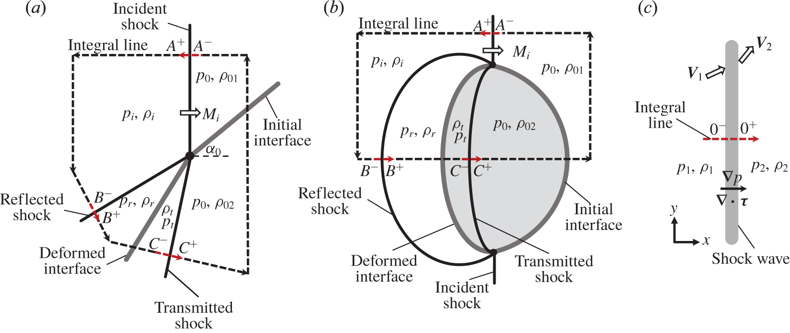
The flow configuration includes a series of shocks in the passing process of the shock through the interface, which is the major process of the circulation deposition in the RMI. The shock wave configuration in the RMI is mainly determined by incident shock Mach number, density ratio across the interface and the initial shape of the gas interface. These critical parameters can be used to determine the flow configuration in the considered region and carry out the integral over the region boundary, as is shown in (1.1). Three shocks, namely, the incident, transmitted and reflected shocks, meet at a single node during regular refraction.
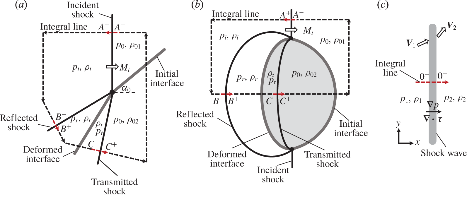
Figure 1(a,b) demonstrates typical RMI problems of regular refraction, which are the fast–slow interface RMI problem and the shock–heavy bubble interaction. The densities of the unshocked gases are  $\unicode[STIX]{x1D70C}_{01}$ and
 $\unicode[STIX]{x1D70C}_{02}$ respectively. There is equal pressure
 $p_{0}$ and temperature
 $T_{0}$ across the unshocked gas interface. The subscripts
 $i$,
 $r$,
 $t$ represent the flow quantities after the incident, reflected and transmitted shocks, respectively. The dashed lines with arrows are the region boundaries along which the circulation is considered.
Schematic of (a) the fast/slow interface RMI, (b) the shock–heavy bubble interaction and (c) the considered single-shock problem.
The circulation rate mainly depends on the gradients of  $p$ and
 $\unicode[STIX]{x1D70F}$, as is shown in (1.1). Thus, we further simplify the calculation by considering the gradient only inside the shocks. For instance, in the circumstance shown in figure 1, we only carry out the integral as (1.1) from
 $A^{-}$ to
 $A^{+}$, from
 $B^{-}$ to
 $B^{+}$ and from
 $C^{-}$ to
 $C^{+}$, which are the red parts on the integral lines in figure 1(a,b). Then, we add them together for the calculation of circulation deposition. We can set the integral line at
 $A,B,C$ perpendicular to each shock at the intersection with each shock, as illustrated in figure 1, which is also the direction of the gradients of flow quantities inside the shocks. The integral in (1.1) does not depend on the direction of the integral line at the location of each shock.
Thus, the fundamental problem is to carry out the integrals across a single shock, as is illustrated in figure 1(c) to calculate the integrals in (1.1). For simplicity, the integral across the shock is in the frame of the shock and the  $x$ axis is chosen to be perpendicular to the shock with the shock located at
 $x=0$. Here,
 $0^{-}$ and
 $0^{+}$ represent the left and right boundaries of the shock, respectively.
The curvature of the shock in the small region of the integral, which leads to the tangential gradient of quantities inside the shock, is ignored. The vorticity jump across a steady shock with a uniform inflow is proportional to the shock curvature (Kevlahan Reference Kevlahan1997). In most RMI cases of practical significance, the shock curvature is negligible, except for the region of the three-shock intersection (shock–shock kink), which is the main region of vorticity deposition investigated here. The vorticity induced by shock curvature is commonly ignored in previous studies related to the circulation deposition in RMI (for instance, see Samtaney & Zabusky (Reference Samtaney and Zabusky1994), Yang et al. (Reference Yang, Kubota and Zukoski1994)).
The incident flow is assumed to be on the left-hand side of the shock. Otherwise, we only have to change the sign of the integrals. The subscripts ‘ $1$’ and ‘
 $2$’ of flow quantities represent the pre-shock and post-shock conditions, respectively.
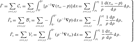
With the integrals inside the incident, transmitted and reflected shocks calculated, equation (1.1) can be expressed as their summation, as shown in (2.1). Here, the problem can be treated as one-dimensional. In a flow quantity  $Q$, we have
 $\unicode[STIX]{x1D735}Q=\text{d}Q/\text{d}x$. The subscripts
 $i,r$ and
 $t$ represent the incident, reflected and transmitted shocks respectively. We change the variable of integration from
 $x$ to
 $\unicode[STIX]{x1D70C}$ in (2.1):
 $$\begin{eqnarray}\left.\begin{array}{@{}c@{}}\displaystyle \dot{\unicode[STIX]{x1D6E4}}=\mathop{\sum }_{s=i,r,t}{\mathcal{C}}_{s}=\mathop{\sum }_{s=i,r,t}\int _{0^{-}}^{0^{+}}[\unicode[STIX]{x1D70C}^{-1}\unicode[STIX]{x1D735}(\unicode[STIX]{x1D70F}_{xx}-p)]\,\text{d}x=\mathop{\sum }_{s=i,r,t}\int _{\unicode[STIX]{x1D70C}_{1}}^{\unicode[STIX]{x1D70C}_{2}}\frac{1}{\unicode[STIX]{x1D70C}}\frac{\text{d}(\unicode[STIX]{x1D70F}_{xx}-p)}{\text{d}\unicode[STIX]{x1D70C}}\,\text{d}\unicode[STIX]{x1D70C},\\ \displaystyle \dot{\unicode[STIX]{x1D6E4}}_{b}=\mathop{\sum }_{s=i,r,t}{\mathcal{B}}_{s}=\mathop{\sum }_{s=i,r,t}-\int _{0^{-}}^{0^{+}}(\unicode[STIX]{x1D70C}^{-1}\unicode[STIX]{x1D735}p)\,\text{d}x=\mathop{\sum }_{s=i,r,t}-\int _{\unicode[STIX]{x1D70C}_{1}}^{\unicode[STIX]{x1D70C}_{2}}\frac{1}{\unicode[STIX]{x1D70C}}\frac{\text{d}p}{\text{d}\unicode[STIX]{x1D70C}}\,\text{d}\unicode[STIX]{x1D70C},\\ \displaystyle \dot{\unicode[STIX]{x1D6E4}}_{v}=\mathop{\sum }_{s=i,r,t}{\mathcal{V}}_{s}=\mathop{\sum }_{s=i,r,t}\int _{0^{-}}^{0^{+}}(\unicode[STIX]{x1D70C}^{-1}\unicode[STIX]{x1D735}\unicode[STIX]{x1D70F}_{xx})\,\text{d}x=\mathop{\sum }_{s=i,r,t}\int _{\unicode[STIX]{x1D70C}_{1}}^{\unicode[STIX]{x1D70C}_{2}}\frac{1}{\unicode[STIX]{x1D70C}}\frac{\text{d}\unicode[STIX]{x1D70F}_{xx}}{\text{d}\unicode[STIX]{x1D70C}}\,\text{d}\unicode[STIX]{x1D70C}.\end{array}\right\}\end{eqnarray}$$
In (2.1), the concept of the circulation rate, baroclinic source and viscous source integrals of a single shock are introduced as  ${\mathcal{C}}_{s}$,
 ${\mathcal{B}}_{s}$ and
 ${\mathcal{V}}_{s}$, respectively. Their calculation is the fundamental problem to be solved to provide the total circulation rate and discover the actual contribution of the viscous source to the circulation deposition. It can be seen in (2.1) that
 ${\mathcal{C}}_{s}$,
 ${\mathcal{B}}_{s}$ and
 ${\mathcal{V}}_{s}$ can be calculated as long as the profiles of
 $(\unicode[STIX]{x1D70C},\unicode[STIX]{x1D70F}_{xx}-p)$,
 $(\unicode[STIX]{x1D70C},p)$ and
 $(\unicode[STIX]{x1D70C},\unicode[STIX]{x1D70F}_{xx})$ inside a shock are predicted. We call this problem the ‘single-shock problem’ and discuss it in the next section.
In (2.1), non-zero values of  ${\mathcal{C}}_{s}$,
 ${\mathcal{B}}_{s}$ and
 ${\mathcal{V}}_{s}$ can be observed on the circulation boundary at the three shocks. However, this notion does not mean that the vorticity is locally generated by these planar shocks. The circulation rate and baroclinic and viscous sources for a specific RMI problem are obtained by adding the integrals together as shown in (2.1). In figure 1, the values of
 ${\mathcal{C}}_{s}$,
 ${\mathcal{B}}_{s}$ and
 ${\mathcal{V}}_{s}$ of the incident and transmitted shocks are opposite in sign. Thus, the circulation is not generated by the planar shocks, but by the difference in the shock strength along the region boundary.
The basis of the prediction of circulation deposition in this investigation is the circulation dynamic equation as (1.1). Such an expression is equivalent to the vorticity dynamic equation (Zabusky Reference Zabusky1999) by employing the surface integral and Green’s theorem on both sides of the vorticity dynamic equation. The vortex-stretching term in the vorticity dynamic equation is absent because we consider a two-dimensional flow here. The combination of the dilatation term  $\unicode[STIX]{x1D714}(\unicode[STIX]{x1D735}\boldsymbol{\cdot }\boldsymbol{V})$ with the convective derivative of vorticity
 $(\boldsymbol{V}\boldsymbol{\cdot }\unicode[STIX]{x1D735})\unicode[STIX]{x1D714}$ leads to term
 $\unicode[STIX]{x1D735}\boldsymbol{\cdot }(\boldsymbol{V}\unicode[STIX]{x1D714})$. This term reflects the vorticity transport across the circulation boundary, and it is not the source of circulation generation. It cannot change the circulation along a material curve and does not exist in (1.1).
3 Single-shock problem
3.1 Circulation rate integral
The normal shock is considered first. The relation between  $\unicode[STIX]{x1D70C}$ and
 $(\unicode[STIX]{x1D70F}_{xx}-p)$ inside the shock should be provided to obtain the circulation rate integral
 ${\mathcal{C}}_{s}$. Here, the conservation of mass and momentum across a stationary normal shock, as shown in (3.1) and (3.2), is used. In these equations,
 $u$ is the velocity in
 $x$ direction:
 $$\begin{eqnarray}\displaystyle & \displaystyle \unicode[STIX]{x1D70C}u=\unicode[STIX]{x1D70C}_{1}u_{1}, & \displaystyle\end{eqnarray}$$
 $$\begin{eqnarray}\displaystyle & \displaystyle \unicode[STIX]{x1D70C}u^{2}+p-\unicode[STIX]{x1D70F}_{xx}=\unicode[STIX]{x1D70C}_{1}{u_{1}}^{2}+p_{1}. & \displaystyle\end{eqnarray}$$
Inserting (3.1) into (3.2), we obtain the governing equation for  $\unicode[STIX]{x1D70C}$ and
 $(\unicode[STIX]{x1D70F}_{xx}-p)$ as
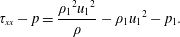 $$\begin{eqnarray}\unicode[STIX]{x1D70F}_{xx}-p=\frac{{\unicode[STIX]{x1D70C}_{1}}^{2}{u_{1}}^{2}}{\unicode[STIX]{x1D70C}}-\unicode[STIX]{x1D70C}_{1}{u_{1}}^{2}-p_{1}.\end{eqnarray}$$
Thus, the integral in (2.1) is expressed as
 $$\begin{eqnarray}{\mathcal{C}}_{s}=\int _{\unicode[STIX]{x1D70C}_{1}}^{\unicode[STIX]{x1D70C}_{2}}\frac{1}{\unicode[STIX]{x1D70C}}\frac{\text{d}(\unicode[STIX]{x1D70F}_{xx}-p)}{\text{d}\unicode[STIX]{x1D70C}}\,\text{d}\unicode[STIX]{x1D70C}=\int _{\unicode[STIX]{x1D70C}_{1}}^{\unicode[STIX]{x1D70C}_{2}}-\frac{{\unicode[STIX]{x1D70C}_{1}}^{2}{u_{1}}^{2}}{\unicode[STIX]{x1D70C}^{3}}\,\text{d}\unicode[STIX]{x1D70C}=\frac{{u_{1}}^{2}}{2}\left(\,\frac{1}{{f_{\unicode[STIX]{x1D70C}}}^{2}}-1\right),\end{eqnarray}$$
where  $f_{\unicode[STIX]{x1D70C}}=\unicode[STIX]{x1D70C}_{2}/\unicode[STIX]{x1D70C}_{1}$ is the density ratio across the shock wave given by the Rankine–Hugoniot shock relation
 $$\begin{eqnarray}f_{\unicode[STIX]{x1D70C}}=\frac{(\unicode[STIX]{x1D6FE}+1){M_{s}}^{2}}{(\unicode[STIX]{x1D6FE}-1){M_{s}}^{2}+2}.\end{eqnarray}$$
Here,  $M_{s}$ is the Mach number of the shock and
 $\unicode[STIX]{x1D6FE}$ is the specific heat ratio;
 ${u_{1}}^{2}$ can be expressed with the shock Mach number
 $M_{s}$ and the pre-shock speed of sound as
 $$\begin{eqnarray}{u_{1}}^{2}=(p_{1}/\unicode[STIX]{x1D70C}_{1})\unicode[STIX]{x1D6FE}{M_{s}}^{2}.\end{eqnarray}$$
By inserting (3.5) and (3.6) into (3.4), the normalised circulation rate integral  ${\mathcal{C}}_{s}^{\ast }$ for a single shock wave is obtained as
 $$\begin{eqnarray}{\mathcal{C}}_{s}^{\ast }=(\unicode[STIX]{x1D70C}_{1}/p_{1}){\mathcal{C}}_{s}=2\unicode[STIX]{x1D6FE}(\unicode[STIX]{x1D6FE}+1)^{-2}(-\unicode[STIX]{x1D6FE}M_{s}^{2}+M_{s}^{-2}+\unicode[STIX]{x1D6FE}-1).\end{eqnarray}$$
The above-mentioned derivation of the normal shock can be easily extended to the oblique shock. The zero gradient of velocity in the  $y$ direction is obtained due to momentum conservation in the
 $y$ direction as long as the
 $x$ axis is chosen to be perpendicular to the oblique shock and the shock curvature is ignored. The conservation of mass and momentum in
 $x$ direction across the oblique shock is the same as for the normal shock in (3.1) and (3.2). Thus, equation (3.7) is still applicable as long as
 $M_{s}$ is replaced by
 $M_{s,n}$, which is the Mach number normal to the oblique shock.
The above-derived calculation of the circulation rate integral  ${\mathcal{C}}_{s}$ combines the pressure
 $p$ and the viscous stress
 $\unicode[STIX]{x1D70F}_{xx}$ together and uses the basic conservation laws of mass and momentum to carry out the integral across the shock, as shown in (3.4). This process does not distinguish the effects of
 $p$ and
 $\unicode[STIX]{x1D70F}_{xx}$. Thus, the relative magnitudes do not change the prediction of
 ${\mathcal{C}}_{s}$. Similarly, in (2.1), the relative magnitudes of baroclinic and viscous sources
 $\dot{\unicode[STIX]{x1D6E4}}_{b}$ and
 $\dot{\unicode[STIX]{x1D6E4}}_{v}$ do not change the prediction of circulation rate
 $\dot{\unicode[STIX]{x1D6E4}}$, which combines different sources together without distinguishing them. In this study, we should distinguish these sources and individually calculate the baroclinic and viscous source integrals of a single shock
 ${\mathcal{B}}_{s}$ and
 ${\mathcal{V}}_{s}$. Such tasks are essential to further reveal the contributions of different mechanisms (baroclinicity and viscosity) to the circulation deposition. The following subsection deals with this aspect.
3.2 Viscous source integral
The viscous source integral of a single shock  ${\mathcal{V}}_{s}$ is predicted theoretically as long as the relation between the density
 $\unicode[STIX]{x1D70C}$ and viscous stress
 $\unicode[STIX]{x1D70F}_{xx}$ inside the shock is obtained. Here, the energy conservation across the normal shock is regarded as
 $$\begin{eqnarray}(E+p-\unicode[STIX]{x1D70F}_{xx})u+q=(E_{1}+p_{1})u_{1},\end{eqnarray}$$
where Fourier’s law for heat conduction is used to calculate for heat transfer  $q$ as below and
 $k$ is the thermal conductivity:
 $$\begin{eqnarray}q=-k\unicode[STIX]{x1D735}T.\end{eqnarray}$$
The state equation of ideal gas is employed to calculate the temperature  $T$ and the total energy
 $E$, as shown in (3.10) and (3.11), where
 $R$ is the gas constant. In (3.10), the mass and momentum conservation, as shown in (3.1) and (3.2), are inserted:
 $$\begin{eqnarray}\displaystyle & \displaystyle T=\frac{p}{R\unicode[STIX]{x1D70C}}=\frac{1}{R}\left(\frac{\unicode[STIX]{x1D70C}_{1}{u_{1}}^{2}+p_{1}}{\unicode[STIX]{x1D70C}}-\frac{{\unicode[STIX]{x1D70C}_{1}}^{2}{u_{1}}^{2}}{\unicode[STIX]{x1D70C}^{2}}+\frac{\unicode[STIX]{x1D70F}_{xx}}{\unicode[STIX]{x1D70C}}\right), & \displaystyle\end{eqnarray}$$
 $$\begin{eqnarray}\displaystyle & \displaystyle E=\frac{p}{\unicode[STIX]{x1D6FE}-1}+\frac{1}{2}\unicode[STIX]{x1D70C}u^{2}. & \displaystyle\end{eqnarray}$$
Then, the temperature gradient is obtained as
 $$\begin{eqnarray}\unicode[STIX]{x1D735}T=\frac{1}{R}\left[-\frac{(\unicode[STIX]{x1D70C}_{1}{u_{1}}^{2}+p_{1})}{\unicode[STIX]{x1D70C}^{2}}+\frac{2{\unicode[STIX]{x1D70C}_{1}}^{2}{u_{1}}^{2}}{\unicode[STIX]{x1D70C}^{3}}-\frac{\unicode[STIX]{x1D70F}_{xx}}{\unicode[STIX]{x1D70C}^{2}}+\frac{1}{\unicode[STIX]{x1D70C}}\frac{\text{d}\unicode[STIX]{x1D70F}_{xx}}{\text{d}\unicode[STIX]{x1D70C}}\right]\unicode[STIX]{x1D735}\unicode[STIX]{x1D70C}.\end{eqnarray}$$
As for the thermal conductivity, equation (3.13) is used with the assumption of a constant Prandtl number  $Pr$ throughout the fluid and the constitutive relation of the Newtonian fluid. Here,
 $c_{p}$ is the heat capacity at constant pressure and
 $\unicode[STIX]{x1D707}$ the dynamic viscosity:
 $$\begin{eqnarray}k=\frac{c_{p}}{Pr}\unicode[STIX]{x1D707}=\frac{3c_{p}}{4Pr}\frac{\unicode[STIX]{x1D70F}_{xx}}{\unicode[STIX]{x1D735}u}=-\frac{3c_{p}}{4Pr}\frac{\unicode[STIX]{x1D70C}^{2}\unicode[STIX]{x1D70F}_{xx}}{\unicode[STIX]{x1D70C}_{1}u_{1}\unicode[STIX]{x1D735}\unicode[STIX]{x1D70C}}.\end{eqnarray}$$
By inserting (3.9)–(3.13) into (3.8) and introducing the normalised variables of  $\unicode[STIX]{x1D719}=\unicode[STIX]{x1D70F}_{xx}/p_{1}$ and
 $\unicode[STIX]{x1D709}=\unicode[STIX]{x1D70C}/\unicode[STIX]{x1D70C}_{1}$, the following governing equation for
 $\unicode[STIX]{x1D70C}$ and
 $\unicode[STIX]{x1D70F}_{xx}$ is obtained:
 $$\begin{eqnarray}\frac{\text{d}\unicode[STIX]{x1D719}}{\text{d}\unicode[STIX]{x1D709}}=\frac{\unicode[STIX]{x1D719}}{\unicode[STIX]{x1D709}}+f_{1}(\unicode[STIX]{x1D709})+\frac{f_{2}(\unicode[STIX]{x1D709})}{\unicode[STIX]{x1D719}},\end{eqnarray}$$
where
 $$\begin{eqnarray}\left.\begin{array}{@{}c@{}}\displaystyle f_{1}(\unicode[STIX]{x1D709})=(\unicode[STIX]{x1D6FE}{M_{s}}^{2}+1)\frac{1}{\unicode[STIX]{x1D709}}-\left(\frac{4Pr}{3}+2\unicode[STIX]{x1D6FE}\right){M_{s}}^{2}\frac{1}{\unicode[STIX]{x1D709}^{2}},\\ \displaystyle f_{2}(\unicode[STIX]{x1D709})=\frac{4Pr}{3}\unicode[STIX]{x1D6FE}{M_{s}}^{2}\left[\left(\frac{\unicode[STIX]{x1D6FE}-1}{2}{M_{s}}^{2}+1\right)\frac{1}{\unicode[STIX]{x1D709}}-(\unicode[STIX]{x1D6FE}{M_{s}}^{2}+1)\frac{1}{\unicode[STIX]{x1D709}^{2}}+\frac{\unicode[STIX]{x1D6FE}+1}{2}{M_{s}}^{2}\frac{1}{\unicode[STIX]{x1D709}^{3}}\right].\end{array}\right\}\end{eqnarray}$$
Equation (3.14) is derived from the classical Navier–Stokes–Fourier (NSF) equation set, and we call it the NSF model. The NSF equation set is inaccurate and inapplicable in the solving of shock wave structure (see Gilbarg & Paolucci Reference Gilbarg and Paolucci1953; Liepmann, Narasimha & Chahine Reference Liepmann, Narasimha and Chahine1962; Alsmeyer Reference Alsmeyer1976). Inside a strong shock wave, the gradients of flow quantities are too large; this condition induces the deviation of stress tensor  $\unicode[STIX]{x1D749}$ and heat flux
 $\boldsymbol{q}$ from the linear Newtonian and Fourier laws (Paolucci & Paolucci Reference Paolucci and Paolucci2018).
Considerable effort has been paid to modifying the NSF equation set to acquire relatively accurate solutions for shock structures. Comprehensive reviews of them can be found in the recent literature (Paolucci & Paolucci Reference Paolucci and Paolucci2018; Uribe & Velasco Reference Uribe and Velasco2018).
In consideration of the simplicity and accuracy amongst those different modifications, we provide a modification of our previous model mainly based on the so-called ‘two-velocity theory’. It was introduced by Brenner (Reference Brenner2005a,Reference Brennerb, Reference Brenner2009) and verified comprehensively for a large range of shock wave Mach numbers by Greenshields & Reese (Reference Greenshields and Reese2007).
The two-velocity theory argues that the deviation of mass velocity  $\boldsymbol{V}_{m}$ and volume velocity
 $\boldsymbol{V}_{v}$ in the region with large mass density gradient is large, and the velocity appearing in Newton’s viscosity law should be
 $\boldsymbol{V}_{v}$ instead of
 $\boldsymbol{V}_{m}$. The relation between
 $\boldsymbol{V}_{v}$ and
 $\boldsymbol{V}_{m}$ for a single component fluid undergoing heat transfer is
 $$\begin{eqnarray}\boldsymbol{V}_{v}=\boldsymbol{V}_{m}+(\unicode[STIX]{x1D6FC}/\unicode[STIX]{x1D70C})\unicode[STIX]{x1D735}\unicode[STIX]{x1D70C},\end{eqnarray}$$
where  $\unicode[STIX]{x1D6FC}=\unicode[STIX]{x1D6FC}^{\ast }\unicode[STIX]{x1D708}$ is termed the ‘volume diffusivity’ and
 $\unicode[STIX]{x1D6FC}^{\ast }$ is a factor.
Thus, the modified expression of  $\unicode[STIX]{x1D70F}_{xx}$ across a normal shock is shown as (3.17). Notably,
 $\widetilde{\unicode[STIX]{x1D70F}}_{xx}$ represents the classical form of viscous stress based on the mass velocity
 $\boldsymbol{V}_{m}$:
 $$\begin{eqnarray}\unicode[STIX]{x1D70F}_{xx}={\textstyle \frac{4}{3}}\unicode[STIX]{x1D707}\unicode[STIX]{x1D735}u_{v}=\widetilde{\unicode[STIX]{x1D70F}}_{xx}+{\textstyle \frac{4}{3}}\unicode[STIX]{x1D707}\unicode[STIX]{x1D735}\left[(\unicode[STIX]{x1D6FC}/\unicode[STIX]{x1D70C})\unicode[STIX]{x1D735}\unicode[STIX]{x1D70C}\right],\end{eqnarray}$$
where
 $$\begin{eqnarray}\widetilde{\unicode[STIX]{x1D70F}}_{xx}={\textstyle \frac{4}{3}}\unicode[STIX]{x1D707}\unicode[STIX]{x1D735}u_{m}=-{\textstyle \frac{4}{3}}\unicode[STIX]{x1D707}\unicode[STIX]{x1D70C}_{1}u_{1}\unicode[STIX]{x1D70C}^{-2}\unicode[STIX]{x1D735}\unicode[STIX]{x1D70C}.\end{eqnarray}$$
Combining (3.17) and (3.18) yields an differential equation for  $\unicode[STIX]{x1D70C}$,
 $\widetilde{\unicode[STIX]{x1D70F}}_{xx}$ and
 $\unicode[STIX]{x1D70F}_{xx}$ as follows:
 $$\begin{eqnarray}\unicode[STIX]{x1D70F}_{xx}=\widetilde{\unicode[STIX]{x1D70F}}_{xx}+\frac{3\unicode[STIX]{x1D6FC}^{\ast }}{4\unicode[STIX]{x1D70C}_{1}^{2}u_{1}^{2}}\unicode[STIX]{x1D70C}^{2}\widetilde{\unicode[STIX]{x1D70F}}_{xx}\frac{\text{d}\widetilde{\unicode[STIX]{x1D70F}}_{xx}}{\text{d}\unicode[STIX]{x1D70C}}.\end{eqnarray}$$
An extra term exists in the energy conservation equation due to the diffusive volume flux (Greenshields & Reese Reference Greenshields and Reese2007). Thus, the energy conservation equation should be modified as (3.20). The thermal conductivity  $k$ can still be calculated as (3.13) as long as
 $\unicode[STIX]{x1D70F}_{xx}$ is replaced by
 $\widetilde{\unicode[STIX]{x1D70F}}_{xx}$:
 $$\begin{eqnarray}(E+p-\unicode[STIX]{x1D70F}_{xx})u-k\unicode[STIX]{x1D735}T-(\unicode[STIX]{x1D6FC}p/\unicode[STIX]{x1D70C})\unicode[STIX]{x1D735}\unicode[STIX]{x1D70C}=(E_{1}+p_{1})u_{1}.\end{eqnarray}$$
Again, the dimensionless variable  $\unicode[STIX]{x1D712}=\widetilde{\unicode[STIX]{x1D70F}}_{xx}/p_{1}$ is introduced. Combining (3.10)–(3.13) and (3.17)–(3.20) leads to the following differential equations:
 $$\begin{eqnarray}\left.\begin{array}{@{}c@{}}\displaystyle \frac{\text{d}\unicode[STIX]{x1D712}}{\text{d}\unicode[STIX]{x1D709}}=\frac{4\unicode[STIX]{x1D6FE}{M_{s}}^{2}}{3\unicode[STIX]{x1D6FC}^{\ast }}\frac{1}{\unicode[STIX]{x1D709}^{2}}\left(\frac{\unicode[STIX]{x1D719}}{\unicode[STIX]{x1D712}}-1\right),\\ \displaystyle \frac{\text{d}\unicode[STIX]{x1D719}}{\text{d}\unicode[STIX]{x1D709}}=f_{1}(\unicode[STIX]{x1D709})\unicode[STIX]{x1D719}+f_{2}(\unicode[STIX]{x1D709})+f_{3}(\unicode[STIX]{x1D709})\frac{1}{\unicode[STIX]{x1D712}}+f_{4}(\unicode[STIX]{x1D709})\frac{\unicode[STIX]{x1D719}}{\unicode[STIX]{x1D712}},\end{array}\right\}\end{eqnarray}$$
where
 $$\begin{eqnarray}\left.\begin{array}{@{}c@{}}\displaystyle f_{1}(\unicode[STIX]{x1D709})=\left(1-\unicode[STIX]{x1D6FC}^{\ast }Pr\frac{\unicode[STIX]{x1D6FE}-1}{\unicode[STIX]{x1D6FE}}\right)\frac{1}{\unicode[STIX]{x1D709}},\\ \displaystyle f_{2}(\unicode[STIX]{x1D709})=\left(1-\unicode[STIX]{x1D6FC}^{\ast }Pr\frac{\unicode[STIX]{x1D6FE}-1}{\unicode[STIX]{x1D6FE}}\right)(\unicode[STIX]{x1D6FE}{M_{s}}^{2}+1)\frac{1}{\unicode[STIX]{x1D709}}-[2\unicode[STIX]{x1D6FE}-\unicode[STIX]{x1D6FC}^{\ast }Pr(\unicode[STIX]{x1D6FE}-1)]{M_{s}}^{2}\frac{1}{\unicode[STIX]{x1D709}^{2}},\\ \displaystyle f_{3}(\unicode[STIX]{x1D709})=\frac{4Pr}{3}\unicode[STIX]{x1D6FE}{M_{s}}^{2}\left[\left(\frac{\unicode[STIX]{x1D6FE}-1}{2}{M_{s}}^{2}+1\right)\frac{1}{\unicode[STIX]{x1D709}}-(\unicode[STIX]{x1D6FE}{M_{s}}^{2}+1)\frac{1}{\unicode[STIX]{x1D709}^{2}}+\frac{\unicode[STIX]{x1D6FE}+1}{2}{M_{s}}^{2}\frac{1}{\unicode[STIX]{x1D709}^{3}}\right],\\ \displaystyle f_{4}(\unicode[STIX]{x1D709})=-\frac{4Pr}{3}{M_{s}}^{2}\frac{1}{\unicode[STIX]{x1D709}^{2}}.\end{array}\right\}\end{eqnarray}$$
According to the original two-velocity theory, we need two differential equations to govern the relation between  $\unicode[STIX]{x1D70C}$ and
 $\unicode[STIX]{x1D70F}_{xx}$. This model is considerably more complex than the previous NSF model. And what is worse is that the robustness of this model depends mainly on the value of the volume diffusivity factor
 $\unicode[STIX]{x1D6FC}^{\ast }$. An unphysical pre-shock overshoot will be obtained for
 $\unicode[STIX]{x1D6FC}^{\ast }\gtrsim 1.45$ according to the spatial stability test by Greenshields & Reese (Reference Greenshields and Reese2007).
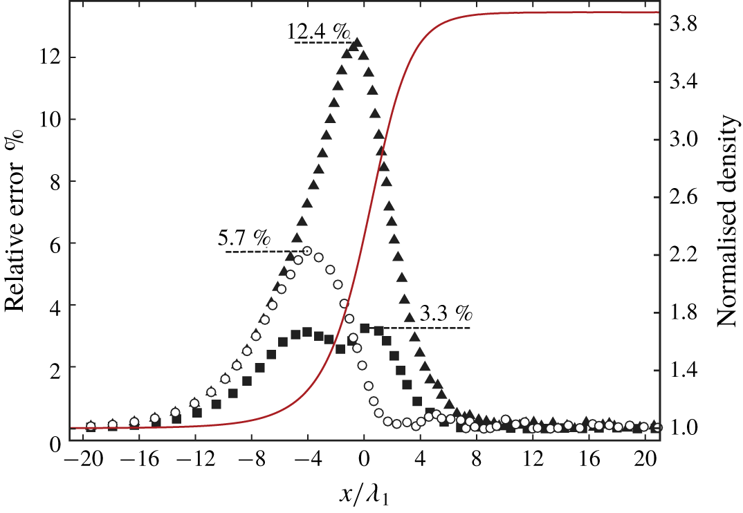
Greenshields & Reese (Reference Greenshields and Reese2007) argued that the unphysical behaviour should be attributed to the presence of the extra term in the momentum flux but not in the energy flux. We further test the relative errors of the momentum and energy equation for the classical NSF equation set as (3.2) and (3.8) using the direct simulation Monte Carlo (DSMC) simulation results of a strong normal shock wave in argon with  $M_{s}=10$. The results are shown in the next subsection. The maximum relative error of momentum given by the classical NSF equation set compared with the pre-shock value is found to be approximately 3 %, whereas it is approximately 13 % for the energy equation.
Thus, the failure of the classical NSF equation set inside the strong shock wave mainly comes from the energy flux, and the unphysical behaviour of the two-velocity theory mainly comes from the momentum flux. Accordingly, we provide our ‘two-velocity NSF’ (TNSF) model by considering only the extra diffusive volume flux term in energy conservation equation given by two-velocity theory and retain the original momentum equation.
With the calculation of  $\unicode[STIX]{x1D70F}_{xx}$ according to the linear Newtonian law and mass conservation equation, we can calculate the extra diffusive volume term in the energy conservation equation as follows:
 $$\begin{eqnarray}\displaystyle & \displaystyle \unicode[STIX]{x1D70F}_{xx}={\textstyle \frac{4}{3}}\unicode[STIX]{x1D707}\unicode[STIX]{x1D735}u=-{\textstyle \frac{4}{3}}\unicode[STIX]{x1D70C}_{1}u_{1}\unicode[STIX]{x1D707}\unicode[STIX]{x1D70C}^{-2}\unicode[STIX]{x1D735}\unicode[STIX]{x1D70C}, & \displaystyle\end{eqnarray}$$
 $$\begin{eqnarray}\displaystyle & \displaystyle -(\unicode[STIX]{x1D6FC}p/\unicode[STIX]{x1D70C})\unicode[STIX]{x1D735}\unicode[STIX]{x1D70C}=-\unicode[STIX]{x1D6FC}^{\ast }p\unicode[STIX]{x1D707}\unicode[STIX]{x1D70C}^{-2}\unicode[STIX]{x1D735}\unicode[STIX]{x1D70C}=\frac{4}{3}\unicode[STIX]{x1D6FC}^{\ast }\frac{p\unicode[STIX]{x1D70F}_{xx}}{\unicode[STIX]{x1D70C}_{1}u_{1}}. & \displaystyle\end{eqnarray}$$
By inserting (3.10)–(3.13), (3.23) and (3.24) into (3.20), the governing equation for  $\unicode[STIX]{x1D70C}$ and
 $\unicode[STIX]{x1D70F}_{xx}$ is obtained as (3.25) and is named the TNSF model. Here, we use Brenner’s original statement that, for single component fluids undergoing heat transfer,
 $\unicode[STIX]{x1D6FC}$ is the same as the thermal diffusivity, which indicates that
 $\unicode[STIX]{x1D6FC}^{\ast }Pr=1$.
 $$\begin{eqnarray}\frac{\text{d}\unicode[STIX]{x1D719}}{\text{d}\unicode[STIX]{x1D709}}=\frac{\unicode[STIX]{x1D719}}{\unicode[STIX]{x1D6FE}\unicode[STIX]{x1D709}}+f_{1}(\unicode[STIX]{x1D709})+\frac{f_{2}(\unicode[STIX]{x1D709})}{\unicode[STIX]{x1D719}},\end{eqnarray}$$
where
 $$\begin{eqnarray}\left.\begin{array}{@{}c@{}}\displaystyle f_{1}(\unicode[STIX]{x1D709})=\left({M_{s}}^{2}+\frac{1}{\unicode[STIX]{x1D6FE}}\right)\frac{1}{\unicode[STIX]{x1D709}}-\left(\frac{4Pr}{3}+\unicode[STIX]{x1D6FE}+1\right){M_{s}}^{2}\frac{1}{\unicode[STIX]{x1D709}^{2}},\\ \displaystyle f_{2}(\unicode[STIX]{x1D709})=\frac{4Pr}{3}\unicode[STIX]{x1D6FE}{M_{s}}^{2}\left[\left(\frac{\unicode[STIX]{x1D6FE}-1}{2}{M_{s}}^{2}+1\right)\frac{1}{\unicode[STIX]{x1D709}}-(\unicode[STIX]{x1D6FE}{M_{s}}^{2}+1)\frac{1}{\unicode[STIX]{x1D709}^{2}}+\frac{\unicode[STIX]{x1D6FE}+1}{2}{M_{s}}^{2}\frac{1}{\unicode[STIX]{x1D709}^{3}}\right].\end{array}\right\}\end{eqnarray}$$
Compared with the NSF model, the TNSF model has the same complexity and does not require the introduction of new parameters. The accuracy of the quantities concerned is improved significantly, which is illustrated in § 3.4.
With the governing equation of  $\unicode[STIX]{x1D709}$ and
 $\unicode[STIX]{x1D719}$ as (3.14) from the NSF model or (3.25) from the TNSF model, the normalised viscous source integral
 ${\mathcal{V}}_{s}^{\ast }$ for a single shock is expressed as (3.27).
 $$\begin{eqnarray}{\mathcal{V}}_{s}^{\ast }=\frac{\unicode[STIX]{x1D70C}_{1}}{p_{1}}{\mathcal{V}}_{s}=\frac{\unicode[STIX]{x1D70C}_{1}}{p_{1}}\int _{\unicode[STIX]{x1D70C}_{1}}^{\unicode[STIX]{x1D70C}_{2}}\frac{1}{\unicode[STIX]{x1D70C}}\frac{\text{d}\unicode[STIX]{x1D70F}_{xx}}{\text{d}\unicode[STIX]{x1D70C}}\,\text{d}\unicode[STIX]{x1D70C}=\int _{1}^{f_{\unicode[STIX]{x1D70C}}}\frac{1}{\unicode[STIX]{x1D709}}\frac{\text{d}\unicode[STIX]{x1D719}}{\text{d}\unicode[STIX]{x1D709}}\,\text{d}\unicode[STIX]{x1D709}.\end{eqnarray}$$
Again, the theory can be easily extended to oblique shocks. In terms of the conservation of energy, the total energy inside an oblique shock differs from that for a normal shock, as shown in (3.28), due to the presence of  $v_{1}$, which is the velocity in the
 $y$ direction of the shock.
 $$\begin{eqnarray}E=\frac{p}{\unicode[STIX]{x1D6FE}-1}+\frac{1}{2}\unicode[STIX]{x1D70C}(u^{2}+{v_{1}}^{2}).\end{eqnarray}$$
However, if (3.28) is inserted into (3.8), the term  $\unicode[STIX]{x1D70C}_{1}u_{1}{v_{1}}^{2}/2$ exists on both sides and can thus be dropped. In other words, the governing equations of
 $\unicode[STIX]{x1D70F}$ and
 $\unicode[STIX]{x1D70C}$ are unchanged except for the replacement of
 $M_{s}$ by
 $M_{s,n}$. Thus, the circulation rate integral
 ${\mathcal{C}}_{s}^{\ast }$ and the viscous source integral
 ${\mathcal{V}}_{s}^{\ast }$ can be simply calculated for an oblique shock wave as long as
 $M_{s}$ is replaced by the normal Mach number
 $M_{s,n}$. The reason is that the oblique shock can be transformed into a normal shock under an appropriate inertial reference frame.
3.3 Approximation of the TNSF model
In the last subsection, the governing equation of the density and the viscous stress inside a shock is derived theoretically, with which the normalised viscous source integral  ${\mathcal{V}}_{s}^{\ast }$ can be calculated. Equation (3.14) for the NSF model and (3.25) for the TNSF model are Abel equations of the second kind (see Polyanin & Zaitsev Reference Polyanin and Zaitsev2017). The exact solutions for these models are difficult to acquire. Here, we provide an approximate solution of the TNSF model.
We discuss the properties of (3.25). The boundary values of the  $(\unicode[STIX]{x1D709},\unicode[STIX]{x1D719})$ profile are (1,0) and (
 $f_{\unicode[STIX]{x1D70C}},0$) in consideration of the physical nature of a shock wave. The first-order derivative of
 $\unicode[STIX]{x1D719}(\unicode[STIX]{x1D709})$ at the boundaries can also be obtained as
 $$\begin{eqnarray}\unicode[STIX]{x1D719}^{\prime }(\unicode[STIX]{x1D709}_{b})=f_{1}(\unicode[STIX]{x1D709}_{b})+\frac{f_{2}^{\prime }(\unicode[STIX]{x1D709}_{b})}{\unicode[STIX]{x1D719}^{\prime }(\unicode[STIX]{x1D709}_{b})},\end{eqnarray}$$
where  $\unicode[STIX]{x1D709}_{b}=1,f_{\unicode[STIX]{x1D70C}}$ are boundary values of
 $\unicode[STIX]{x1D709}$ and the L’Hopital law is used in the last term. The solutions for
 $\unicode[STIX]{x1D719}^{\prime }(\unicode[STIX]{x1D709}_{b})$ are multi-valued, and the bigger ones are found to agree with our numerical simulations. The values are
 $$\begin{eqnarray}\unicode[STIX]{x1D719}^{\prime }(\unicode[STIX]{x1D709}_{b})={\textstyle \frac{1}{2}}[f_{1}(\unicode[STIX]{x1D709}_{b})+\sqrt{f_{1}(\unicode[STIX]{x1D709}_{b})^{2}+4{f_{2}}^{\prime }(\unicode[STIX]{x1D709}_{b})}],\end{eqnarray}$$
where  $f_{1}(\unicode[STIX]{x1D709}_{b}),{f_{2}}^{\prime }(\unicode[STIX]{x1D709}_{b})$ are calculated from (3.26) as
 $$\begin{eqnarray}\left.\begin{array}{@{}c@{}}\displaystyle f_{1}(1)=-\left(\frac{4Pr}{3}+\unicode[STIX]{x1D6FE}\right){M_{s}}^{2}+\frac{1}{\unicode[STIX]{x1D6FE}},\\ \displaystyle f_{1}(f_{\unicode[STIX]{x1D70C}})=\left({M_{s}}^{2}+\frac{1}{\unicode[STIX]{x1D6FE}}\right)\frac{1}{f_{\unicode[STIX]{x1D70C}}}-\left(\frac{4Pr}{3}+\unicode[STIX]{x1D6FE}+1\right){M_{s}}^{2}\frac{1}{{f_{\unicode[STIX]{x1D70C}}}^{2}},\\ \displaystyle {f_{2}}^{\prime }(1)=-\frac{4Pr}{3}\unicode[STIX]{x1D6FE}{M_{s}}^{2}({M_{s}}^{2}-1),\\ \displaystyle {f_{2}}^{\prime }(f_{\unicode[STIX]{x1D70C}})=\frac{4Pr}{3}\unicode[STIX]{x1D6FE}{M_{s}}^{2}\left[\frac{(1-\unicode[STIX]{x1D6FE}){M_{s}}^{2}-2}{2{f_{\unicode[STIX]{x1D70C}}}^{2}}+\frac{2(\unicode[STIX]{x1D6FE}{M_{s}}^{2}+1)}{{f_{\unicode[STIX]{x1D70C}}}^{3}}-\frac{3(\unicode[STIX]{x1D6FE}+1){M_{s}}^{2}}{2{f_{\unicode[STIX]{x1D70C}}}^{4}}\right].\end{array}\right\}\end{eqnarray}$$
Thus, we have four conditions now, which implies that four free coefficients in the function should be used to estimate the solution of (3.25). Empirically, the function in (3.32) is exploited to satisfy the four conditions. We call this model the ‘TNSF2 model’. The applicability and accuracy of this model are illustrated in § 3.4:
 $$\begin{eqnarray}\unicode[STIX]{x1D719}=C_{1}\unicode[STIX]{x1D709}+C_{2}+C_{3}\unicode[STIX]{x1D709}^{-1}+C_{4}\unicode[STIX]{x1D709}^{-2},\end{eqnarray}$$
where
 $$\begin{eqnarray}\left[\begin{array}{@{}c@{}}C_{1}\\ C_{2}\\ C_{3}\\ C_{4}\end{array}\right]=\frac{1}{(f_{\unicode[STIX]{x1D70C}}-1)^{2}}\left[\begin{array}{@{}c@{}}\unicode[STIX]{x1D719}^{\prime }(1)+{f_{\unicode[STIX]{x1D70C}}}^{2}\unicode[STIX]{x1D719}^{\prime }(f_{\unicode[STIX]{x1D70C}})\\ -(2f_{\unicode[STIX]{x1D70C}}+1)\unicode[STIX]{x1D719}^{\prime }(1)-(f_{\unicode[STIX]{x1D70C}}+2){f_{\unicode[STIX]{x1D70C}}}^{2}\unicode[STIX]{x1D719}^{\prime }(f_{\unicode[STIX]{x1D70C}})\\ (f_{\unicode[STIX]{x1D70C}}+2)f_{\unicode[STIX]{x1D70C}}\unicode[STIX]{x1D719}^{\prime }(1)+(2f_{\unicode[STIX]{x1D70C}}+1){f_{\unicode[STIX]{x1D70C}}}^{2}\unicode[STIX]{x1D719}^{\prime }(f_{\unicode[STIX]{x1D70C}})\\ -{f_{\unicode[STIX]{x1D70C}}}^{2}\unicode[STIX]{x1D719}^{\prime }(1)-{f_{\unicode[STIX]{x1D70C}}}^{3}\unicode[STIX]{x1D719}^{\prime }(f_{\unicode[STIX]{x1D70C}})\end{array}\right].\end{eqnarray}$$
With the aforementioned approximated  $(\unicode[STIX]{x1D709},\unicode[STIX]{x1D719})$ profile, the normalised viscous source integral
 ${\mathcal{V}}_{s}^{\ast }$ is acquired from (3.27) as
 $$\begin{eqnarray}{\mathcal{V}}_{s}^{\ast }=\left[\frac{\ln (f_{\unicode[STIX]{x1D70C}})}{(f_{\unicode[STIX]{x1D70C}}-1)^{2}}+\frac{{f_{\unicode[STIX]{x1D70C}}}^{2}-5f_{\unicode[STIX]{x1D70C}}-2}{6f_{\unicode[STIX]{x1D70C}}(f_{\unicode[STIX]{x1D70C}}-1)}\right]\unicode[STIX]{x1D719}^{\prime }(1)+\left[\frac{{f_{\unicode[STIX]{x1D70C}}}^{2}\ln (f_{\unicode[STIX]{x1D70C}})}{(f_{\unicode[STIX]{x1D70C}}-1)^{2}}-\frac{2{f_{\unicode[STIX]{x1D70C}}}^{2}+5f_{\unicode[STIX]{x1D70C}}-1}{6(f_{\unicode[STIX]{x1D70C}}-1)}\right]\unicode[STIX]{x1D719}^{\prime }(f_{\unicode[STIX]{x1D70C}}).\end{eqnarray}$$
3.4 Single-shock simulations
The numerical simulations of single shocks are carried out to verify the above-mentioned derivations. The DSMC method (Bird Reference Bird1994), which is the general simulation method in investigations of shock wave structures, is used in the numerical simulations. The data from the DSMC simulations are always taken for comparison due to the difficulty in measuring the flow quantities (except for density) inside a shock wave (see Bird Reference Bird1970; Alsmeyer Reference Alsmeyer1976; Lumpkin III & Chapman Reference Lumpkin and Chapman1992; Greenshields & Reese Reference Greenshields and Reese2007; Uribe & Velasco Reference Uribe and Velasco2018).
In the DSMC method, the Boltzmann equation is solved with a particle-based stochastic algorithm and the continuous molecular velocity distribution function is estimated by a discrete number of computational molecules. The physical domain is discretised into cells, each of which contains some computational particles. Each computational particle represents a large number  $N_{p}$ of real particles. The motions and collisions of these computational particles are simulated. At every time step
 $\unicode[STIX]{x0394}t$, the translation of the computational particles is simulated first. Then, the simulation of the collision process of particle pairs is carried out, in which the selection of particles for collision is random.
As for the DSMC method for steady flow, the number of time steps for a steady stage is  $N_{s0}$, after which the flow in the computational domain reaches a steady state. In the steady stage, the number of time steps, which is also the time of sampling, is
 $N_{s}$. The sampling of the properties of particles in a cell during the steady stage determines the macroscopic gas properties
 $(\boldsymbol{V},p,T,\unicode[STIX]{x1D70C},\unicode[STIX]{x1D749})$. The results of the DSMC method theoretically tend towards the real performance of a gas at the molecular scale as long as
 $N_{s}$ is sufficiently large and
 $N_{p}$ is sufficiently small.
Here, we use the DSMC1S.FOR (Bird Reference Bird1994, pp. 286–305) code to simulate the shock wave structure. The computational domain is  $x\in (-x_{0},x_{0})$ and the shock wave is initially located at
 $x_{s}=0$. Initially, the upstream and downstream properties, which are determined by the Rankine–Hugoniot shock relation, are given in the regions
 $x<0$ and
 $x>0$, respectively. This condition indicates that the shock wave is a discontinuity initially and develops into a physically meaningful shock wave during the unsteady phase of the calculation.
The left boundary is inflow boundary, and the uniform upstream condition is used. For the right boundary, the boundary condition is set as a specularly reflecting wall that moves with the velocity  $u_{d}$ equal to the downstream Rankine–Hugoniot velocity. At every time step, the wall ‘jumps’ back to
 $x=x_{0}$ after interacting with the particle. This boundary condition reduces the random walk of the shock wave significantly, which is mainly caused by the fluctuation in the particle number exiting the subsonic downstream boundary.
Another operation is run to eliminate the random walk of the shock wave. This operation is a single subroutine that monitors the total particle number in the computational domain. If the number deviates from the initial number more than a specific small number, then all the particles are displaced by a same distance, after which the total particle number is restored to the initial value. With this operation, the shock wave is nearly stable at  $x=0$ during the whole computational time.
In the present study, all the simulations are about monatomic gases due to their considerably simpler thermodynamic behaviour than that of polyatomic gases. Monatomic gases possess no modes of rotation or vibration and only ionise at the highest temperatures. The effect of dissociation chemistry has been comprehensively investigated by Samtaney & Meiron (Reference Samtaney and Meiron1997) but is out of the scope of this study. This effect is inherently absent in monatomic gases. Additionally, we find that the selection of the collision models for a monatomic gas in the simulation does not influence the simulation results, particularly the  $(\unicode[STIX]{x1D70C},\unicode[STIX]{x1D70F})$ profile inside the shock wave.
Normal shock waves in argon of different strength  $M_{s}\in [1.5,10]$ are simulated, and the interval is
 $\unicode[STIX]{x0394}M_{s}=0.5$. The properties of argon are listed in Bird (Reference Bird1994). The upstream condition is the same as the popular experimental database provided by Alsmeyer (Reference Alsmeyer1976), which is
 $p_{1}=6.67~\text{N}~\text{m}^{-2}$ and
 $T_{1}=300~\text{K}$. The computational domain is
 $x\in (-0.03,0.03)~\text{m}$ and is divided into 600 cells. The cell size and time step are
 $\unicode[STIX]{x0394}x=10^{-4}~\text{m}$ and
 $\unicode[STIX]{x0394}t=2\times 10^{-8}~\text{s}$, respectively. The number of time steps for the flow to reach the steady stage
 $N_{s0}$ and the following times of sampling
 $N_{s}$ are
 $10^{5}$ and
 $10^{6}$, respectively. One computational particle represents
 $N_{p}=3\times 10^{15}$ real particles. The variable hard sphere (VHS) model is selected as the collision model. The verifications and validations of our simulations are illustrated in appendix A.
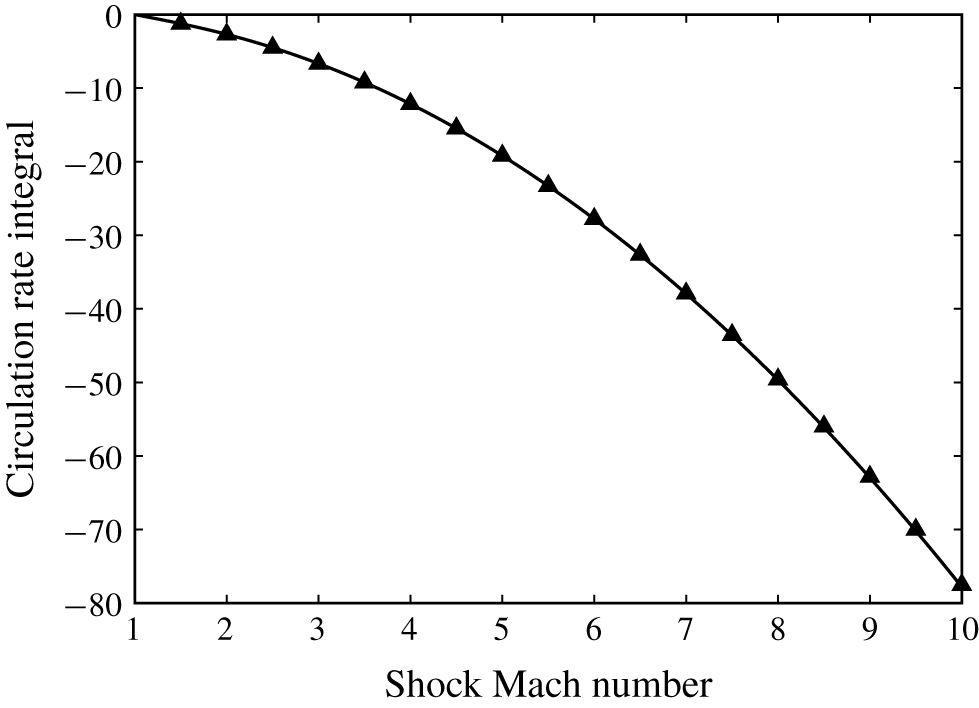
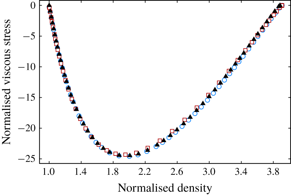
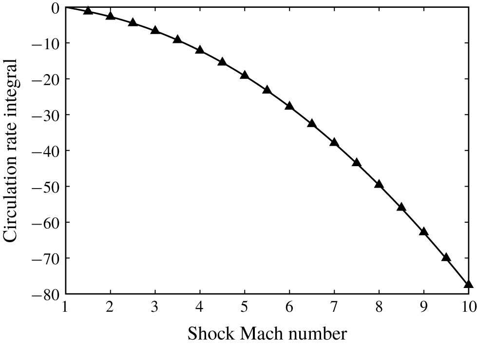
Firstly, the prediction of the circulation rate integral  ${\mathcal{C}}_{s}^{\ast }$ for a single shock as (3.7) is validated. Figure 2 illustrates the comparison of the circulation rate integral for normal shocks with different strengths between the predictions by (3.7) and the DSMC simulated results. For DSMC results, the integral in (3.4) is obtained numerically with the trapezoidal rule.
As demonstrated in figure 2, the theoretical predictions agree with the numerical results quite well within a wide range of shock Mach numbers (from 1 to 10). Therefore, our theoretical prediction of the circulation rate integral  ${\mathcal{C}}_{s}^{\ast }$ for a single shock is accurate.
Comparison of the circulation rate integral of a normal shock in argon between the present model as (3.7) and DSMC results. Symbols: ▴, DSMC simulated results; ——, theoretical predictions.
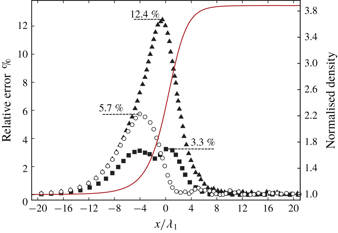
Then, the necessity and reasonability of the TNSF model are investigated. In the previous subsections, we claim that the classical NSF equation set loses its applicability in predicting the density and viscous stress profile for strong normal shocks. Its modification is carried out mainly on the basis of the two-velocity theory. With the modification only used in the energy conservation equation, the TNSF model is obtained. Here, we use the DSMC simulated flow quantities inside a normal shock to demonstrate the relative errors of momentum and energy predicted by the classical NSF or the modified NSF equation set. The momentum and energy relative errors  $\unicode[STIX]{x1D716}_{m}$ and
 $\unicode[STIX]{x1D716}_{e}$ are defined as (3.35) and indirectly explain the necessity and reasonability of the TNSF model:
 $$\begin{eqnarray}\left.\begin{array}{@{}c@{}}\displaystyle \unicode[STIX]{x1D716}_{m}=\left|1-\frac{\unicode[STIX]{x1D70C}u^{2}+p-\unicode[STIX]{x1D70F}_{xx}}{\unicode[STIX]{x1D70C}_{l}u_{l}^{2}+p_{l}}\right|\times 100\,\%,\\ \displaystyle \unicode[STIX]{x1D716}_{e}=\left|1-\frac{\left(E+p-\unicode[STIX]{x1D70F}_{xx}\right)u+q}{\left(E_{l}+p_{l}\right)u_{l}}\right|\times 100\,\%,\end{array}\right\}\end{eqnarray}$$
where the viscous stress  $\unicode[STIX]{x1D70F}_{xx}$ and the heat flux
 $q$ are calculated by (3.36). Here,
 $q_{0}$ and
 $q_{1}$ are the heat fluxes in the classical NSF equation set and the modified one in the TNSF model, respectively. The power law for the viscosity coefficient is used; for argon:
 $T_{0}=273~\text{K},\unicode[STIX]{x1D707}_{0}=2.117\times 10^{-5}~\text{Ns}~\text{m}^{-2},\unicode[STIX]{x1D70E}=0.81$ (Bird Reference Bird1994). Notice that these relative errors reflect the modelling errors of the viscous stress
 $\unicode[STIX]{x1D70F}_{xx}$ and heat flux
 $q$ inside a shock wave. The errors do not represent the inherent physical non-conservation of the momentum and energy inside the shock:
 $$\begin{eqnarray}\left.\begin{array}{@{}c@{}}\displaystyle \unicode[STIX]{x1D70F}_{xx}=\frac{4}{3}\unicode[STIX]{x1D707}\unicode[STIX]{x1D735}u=\frac{4}{3}\unicode[STIX]{x1D707}_{0}\left(\frac{T}{T_{0}}\right)^{\unicode[STIX]{x1D70E}}\unicode[STIX]{x1D735}u,\\ \displaystyle q_{0}=k\unicode[STIX]{x1D735}T=\frac{c_{p}}{Pr}\unicode[STIX]{x1D707}_{0}\left(\frac{T}{T_{0}}\right)^{\unicode[STIX]{x1D70E}}\unicode[STIX]{x1D735}T,\\ \displaystyle q_{1}=q_{0}-1.5\unicode[STIX]{x1D707}_{0}\left(\frac{T}{T_{0}}\right)^{\unicode[STIX]{x1D70E}}\frac{p}{\unicode[STIX]{x1D70C}^{2}}\unicode[STIX]{x1D735}\unicode[STIX]{x1D70C}.\end{array}\right\}\end{eqnarray}$$
The classical NSF equation set meets great challenges in the prediction of a strong shock structure. The DSMC simulated result of a strong shock ( $M_{s}=10$) is taken as an example to reveal the necessity and reasonability of the TNSF model. The phenomenon and conclusions are qualitatively similar in weak shocks. The profiles of momentum and energy relative errors are illustrated in figure 3. For the sake of clarity, the normalised density profile of the shock is also shown. The maximal momentum relative error is approximately 3 % for classical NSF equation set, whereas it is over 12 % for energy. Thus, the decision of modifying only the energy conservation equation in our TNSF model is reasonable and necessary. After modification, the relative error of the energy is significantly decreased, especially in the post-shock regions. The maximal relative error of energy is less than 6 %, which indicates the efficiency of the modification of the energy conservation equation based on two-velocity theory.
Relative errors of momentum and energy conservation calculated from the classical NSF equation set and the modified energy conservation equation for the DSMC result of a Mach 10 shock in argon. Symbols: ▪, momentum; ▲, energy; ○, modified energy; ——, density.
Furthermore, the profile of density  $\unicode[STIX]{x1D70C}$ and viscous stress
 $\unicode[STIX]{x1D70F}_{xx}$ inside a normal shock is considered. In the previous subsections, we claim that the fundamental problem to calculate the viscous source integral for a single shock is to determine the (
 $\unicode[STIX]{x1D70C},\unicode[STIX]{x1D70F}$) profile inside it. The aforementioned derived NSF and TNSF models deal with this problem.
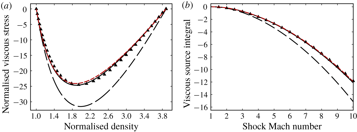
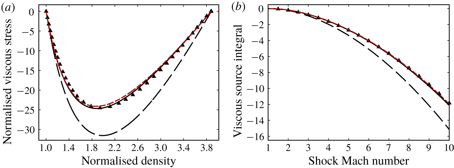
In figure 4(a), the predicted ( $\unicode[STIX]{x1D709},\unicode[STIX]{x1D719}$) profiles are compared with numerical simulated ones for a normal shock in argon with
 $M_{s}=10$. The governing differential equation of the NSF model as (3.14) and TNSF model as equation (3.25) are solved numerically with the Euler method. The number of steps is
 $10^{4}$ and the initial condition is (
 $f_{\unicode[STIX]{x1D70C}},\unicode[STIX]{x1D700}$), where
 $\unicode[STIX]{x1D700}$ is a small value to prevent the denominators of the last terms in (3.14) and (3.25) being zero. Here, we chose
 $\unicode[STIX]{x1D700}=-10^{-4}$. Notably, (
 $\unicode[STIX]{x1D709},\unicode[STIX]{x1D719}$) scarcely depends on the value of
 $\unicode[STIX]{x1D700}$.
The ( $\unicode[STIX]{x1D709},\unicode[STIX]{x1D719}$) profile predicted by the NSF model considerably deviates from the numerically simulated results. This condition indicates the breakdown of the classical NSF equation set inside a strong shock wave. The capability of our TNSF model is proved by the satisfying agreement between the predicted and simulated (
 $\unicode[STIX]{x1D709},\unicode[STIX]{x1D719}$) profiles.
The predicted ( $\unicode[STIX]{x1D709},\unicode[STIX]{x1D719}$) profile by the approximated TNSF model, namely, the TNSF2 model, is also shown in figure 4(a). This model coincides with the exact solution of (3.25) quite well. Therefore, equation (3.32) is suitable as the estimated solution of (3.25). Thus, the equation is acceptable for predicting the (
 $\unicode[STIX]{x1D709},\unicode[STIX]{x1D719}$) profile inside a shock wave.
Predictions from NSF, TNSF and TNSF2 models compared with the DSMC result of (a) the profiles of normalised density  $\unicode[STIX]{x1D709}$ and viscous stress
 $\unicode[STIX]{x1D719}$ of a Mach 10 shock in argon (b) the normalised viscous source integral for normal shocks with different strengths in argon. Symbols: ▲, DSMC simulated results; – –, NSF predictions; ——, TNSF predictions; - - - - - -, TNSF2 predictions.
Thereafter, the normalised viscous source integral  ${\mathcal{V}}_{s}^{\ast }$ for a single shock is also considered. The numerical integral as (3.27) is used to the governing equations of
 $\unicode[STIX]{x1D70C}$ and
 $\unicode[STIX]{x1D70F}_{xx}$ from the NSF and TNSF models and the DSMC simulated result of normal shocks with a Mach number ranging from 1 to 10.
The comparisons between predicted and simulated results are shown in figure 4(b). The viscous source integral predicted by the NSF model deviates from the simulated results increasingly with the increase in shock strength. Unacceptable deviations are observed for strong shocks. For the predictions of the TNSF model, satisfying agreements are obtained in the whole range of shock Mach number (from 1 to 10).
Again, the theoretical predictions by the TNSF2 model are shown in figure 4(b), which is governed by (3.34). They coincide with the exact solution of the TNSF model perfectly. Therefore, the model is convenient and efficient for predicting the viscous source integral for a single shock.
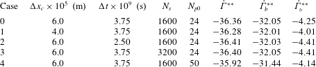
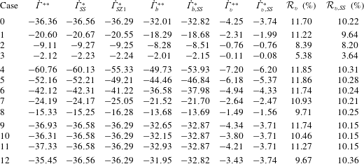
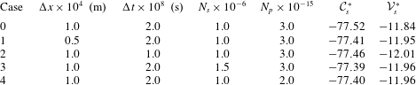
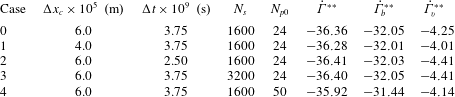
Lastly, the universality of our theory is verified. We simulated normal shocks of  $M_{s}=10$ with different conditions, as listed in table 1. Case 0 is the baseline, which is the case used in the above-mentioned verifications of
 $M_{s}=10$. The pressure and density in case 1 are
 $10^{4}$ times of those in case 0. Thus, case 1 has a considerably thinner shock wave thickness than case 0. Accordingly, the cell size is decreased to
 $\unicode[STIX]{x0394}x=5\times 10^{-9}~\text{m}$, and the time step is decreased to
 $\unicode[STIX]{x0394}t=2\times 10^{-12}~\text{s}$. The total grid and time step numbers are keeping the same as case 0. Case 2 is the normal shock in xenon with the same pre-shock pressure and temperature as case 0. Case 3 is the case of an oblique shock with the strength of
 $M_{s,n}=10$ and the incident flow angle
 $\unicode[STIX]{x1D6FD}=30^{\circ }$.
The normalised circulation rate integral  ${\mathcal{C}}_{s}^{\ast }$ and the normalised viscous source integral
 ${\mathcal{V}}_{s}^{\ast }$ of those cases are listed in table 1. Our theory above indicates that all the cases should have the same values of
 ${\mathcal{C}}_{s}^{\ast }$ and
 ${\mathcal{V}}_{s}^{\ast }$. The numerical results agree well with the theoretical ones. The results for strong shocks (
 $M_{s}=10$) are shown as examples here. We have verified that the universality of our theory also holds for weak shocks.
DSMC simulations of shock waves under different conditions.

4 Predictions of circulation deposition in RMI
4.1 Predictions of RMI with different initial conditions
So far, the circulation rate integral  ${\mathcal{C}}_{s}^{\ast }$ and viscous source integral
 ${\mathcal{V}}_{s}^{\ast }$ for a single shock have been obtained theoretically as (3.7) and (3.34). The circulation rate and viscous source for an RMI problem with specific initial conditions can be easily acquired with the circulation rate integral
 ${\mathcal{C}}_{s}^{\ast }$, the viscous source integral
 ${\mathcal{V}}_{s}^{\ast }$ and the pre-shock density
 $\unicode[STIX]{x1D70C}_{l}$ and pressure
 $p_{l}$ of the incident, transmitted and reflected shocks.
For the regular refraction at the gas interface, the pre-shock density and pressure of the reflected shock are the same as the post-shock density and pressure of the incident shock, which can be obtained using the Rankine–Hugoniot shock relations across the incident shock. Thus, the circulation rate  $\dot{\unicode[STIX]{x1D6E4}}$ and the viscous source
 $\dot{\unicode[STIX]{x1D6E4}}_{v}$ can be expressed as (4.1) and (4.2):
 $$\begin{eqnarray}\displaystyle & \displaystyle \dot{\unicode[STIX]{x1D6E4}}={\mathcal{C}}_{i}-{\mathcal{C}}_{t}+{\mathcal{C}}_{r}=(p_{0}/\unicode[STIX]{x1D70C}_{01})\dot{\unicode[STIX]{x1D6E4}}^{\ast }=(p_{0}/\unicode[STIX]{x1D70C}_{01})\left({\mathcal{C}}_{i}^{\ast }-\unicode[STIX]{x1D702}^{-1}{\mathcal{C}}_{t}^{\ast }+f_{i}{\mathcal{C}}_{r}^{\ast }\right), & \displaystyle\end{eqnarray}$$
 $$\begin{eqnarray}\displaystyle & \displaystyle \dot{\unicode[STIX]{x1D6E4}}_{v}={\mathcal{V}}_{i}-{\mathcal{V}}_{t}+{\mathcal{V}}_{r}=(p_{0}/\unicode[STIX]{x1D70C}_{01})\dot{\unicode[STIX]{x1D6E4}}_{v}^{\ast }=(p_{0}/\unicode[STIX]{x1D70C}_{01})\left({\mathcal{V}}_{i}^{\ast }-\unicode[STIX]{x1D702}^{-1}{\mathcal{V}}_{t}^{\ast }+f_{i}{\mathcal{V}}_{r}^{\ast }\right). & \displaystyle\end{eqnarray}$$
In the above-mentioned equations,  $p_{0}$ is the pre-shock pressure,
 $\unicode[STIX]{x1D70C}_{01}$ is the pre-shock density of the incident gas and
 $\unicode[STIX]{x1D702}=\unicode[STIX]{x1D70C}_{02}/\unicode[STIX]{x1D70C}_{01}$ is the density ratio of the gases across the interface;
 $\dot{\unicode[STIX]{x1D6E4}}^{\ast }$ and
 $\dot{\unicode[STIX]{x1D6E4}}_{v}^{\ast }$ are the normalised circulation rate and viscous source;
 $f_{i}$ is given by the Rankine–Hugoniot shock relations as
 $$\begin{eqnarray}f_{i}=\frac{p_{i}/p_{0}}{\unicode[STIX]{x1D70C}_{i}/\unicode[STIX]{x1D70C}_{01}}=\frac{(2\unicode[STIX]{x1D6FE}_{1}{M_{i}}^{2}-\unicode[STIX]{x1D6FE}_{1}+1)[(\unicode[STIX]{x1D6FE}_{1}-1){M_{i}}^{2}+2]}{(\unicode[STIX]{x1D6FE}_{1}+1)^{2}{M_{i}}^{2}},\end{eqnarray}$$
where  $\unicode[STIX]{x1D6FE}_{1}$ is the specific heat ratio of the incident gas and
 $M_{i}$ is the incident shock strength.
Thus, the shock strength of the transmitted and reflected shocks  $M_{r}$ and
 $M_{t}$ should be determined to predict
 ${\mathcal{V}}_{r,t}^{\ast }$,
 ${\mathcal{C}}_{r,t}^{\ast }$ and then the circulation rate and the viscous source for a specific RMI problem. The two physical conditions of equal pressure and flow direction across the shocked gas interface are used. The shock polar analysis (Henderson Reference Henderson1966) or the twelfth-order polynomial method (Henderson Reference Henderson1964, Reference Henderson1966) are alternative approaches to this problem;
 $M_{r}$ and
 $M_{t}$ are always solved by numerical methods due to the difficulty in providing their exact theoretical solutions (see Henderson Reference Henderson1964).
Here, we give an asymptotic approach to estimate the values of  $M_{r}$ and
 $M_{t}$. With the governing condition of equal pressure after the reflected shock and the transmitted shock, we have
 $$\begin{eqnarray}P_{i}P_{r}=P_{t},\end{eqnarray}$$
where  $P_{i,r,t}$ are the pressure ratios across the incident, reflected and transmitted shocks respectively. They can be written as functions of
 $M_{i,r,t}$. As a result,
 $M_{t}$ as a function of
 $M_{r}$ can be obtained as
 $$\begin{eqnarray}M_{t}(M_{r})=\sqrt{C_{t1}{M_{r}}^{2}+C_{t2}},\end{eqnarray}$$
where
 $$\begin{eqnarray}\left.\begin{array}{@{}c@{}}\displaystyle C_{t1}=\frac{\unicode[STIX]{x1D6FE}_{1}(\unicode[STIX]{x1D6FE}_{2}+1)}{\unicode[STIX]{x1D6FE}_{2}(\unicode[STIX]{x1D6FE}_{1}+1)^{2}}(2\unicode[STIX]{x1D6FE}_{1}{M_{i}}^{2}-\unicode[STIX]{x1D6FE}_{1}+1),\\ \displaystyle C_{t2}=-\frac{(\unicode[STIX]{x1D6FE}_{1}-1)(\unicode[STIX]{x1D6FE}_{2}+1)}{2\unicode[STIX]{x1D6FE}_{2}(\unicode[STIX]{x1D6FE}_{1}+1)^{2}}(2\unicode[STIX]{x1D6FE}_{1}{M_{i}}^{2}-\unicode[STIX]{x1D6FE}_{1}+1)+\frac{\unicode[STIX]{x1D6FE}_{2}-1}{2\unicode[STIX]{x1D6FE}_{2}}.\end{array}\right\}\end{eqnarray}$$
With the Rankine–Hugoniot shock relation for oblique shocks, the deflection angles across the incident, reflected and transmitted shocks  $\unicode[STIX]{x1D703}_{i,r,t}$ are expressed as the functions of
 $M_{i,r,t}$, as shown in (4.7). Here,
 $M_{1i,1r,1t}$ are the flow Mach numbers before the incident, reflected and transmitted shocks under the frame of the three-shock intersection. The local angle between the unshocked gas interface and the horizontal line at the three-shock intersection is
 $\unicode[STIX]{x1D6FC}_{0}$:
 $$\begin{eqnarray}\tan \unicode[STIX]{x1D703}_{i,r,t}=\frac{2\left({M_{i,r,t}}^{2}-1\right)\sqrt{{M_{1i,1r,1t}}^{2}-{M_{i,r,t}}^{2}}}{-2{M_{i,r,t}}^{3}+(\unicode[STIX]{x1D6FE}_{1,2}+1){M_{1i,1r,1t}}^{2}M_{i,r,t}+2M_{i,r,t}},\end{eqnarray}$$
where
 $$\begin{eqnarray}\left.\begin{array}{@{}c@{}}\displaystyle {M_{1i}}^{2}=(\tan ^{2}\unicode[STIX]{x1D6FC}_{0}+1){M_{i}}^{2},\\ \displaystyle {M_{1r}}^{2}=\frac{(\unicode[STIX]{x1D6FE}_{1}+1)^{2}{M_{i}}^{4}\tan ^{2}\unicode[STIX]{x1D6FC}_{0}}{(2\unicode[STIX]{x1D6FE}_{1}{M_{i}}^{2}-\unicode[STIX]{x1D6FE}_{1}+1)[(\unicode[STIX]{x1D6FE}_{1}-1){M_{i}}^{2}+2]}+\frac{(\unicode[STIX]{x1D6FE}_{1}-1){M_{i}}^{2}+2}{2\unicode[STIX]{x1D6FE}_{1}{M_{i}}^{2}-\unicode[STIX]{x1D6FE}_{1}+1},\\ \displaystyle {M_{1t}}^{2}=\frac{\unicode[STIX]{x1D6FE}_{1}}{\unicode[STIX]{x1D6FE}_{2}}(\tan ^{2}\unicode[STIX]{x1D6FC}_{0}+1)\unicode[STIX]{x1D702}{M_{i}}^{2}.\end{array}\right\}\end{eqnarray}$$
The second governing condition of equal flow direction across the gas interface ( $\unicode[STIX]{x1D703}_{i}-\unicode[STIX]{x1D703}_{r}=\unicode[STIX]{x1D703}_{t}$) is also exploited. With some basic algebraic knowledge, the condition is expressed as (4.9). For simplicity, we use ‘
 $T_{i,r,t}$’ to represent the terms ‘
 $\tan \unicode[STIX]{x1D703}_{i,r,t}$’:
 $$\begin{eqnarray}G(M_{r})=T_{r}(M_{r})T_{t}(M_{t})T_{i}+T_{r}(M_{r})+T_{t}(M_{t})-T_{i}=0.\end{eqnarray}$$
Equation (4.9) uses  $M_{r}$ as the variable of the governing equation instead of the pressure ratio across the transmitted shock
 $P_{t}$. Thus, this equation differs from the previous approaches, that is, the shock polar analysis or the twelfth-order polynomial method.
The exact solution of the equation above is difficult to acquire;  $M_{r}$ is slightly higher than
 $1$ for most RMI problems. Thus, we expand
 $G(M_{r})$ at
 $M_{r}=1$ and omit the high-order terms to obtain the approximation of
 $M_{r}$ as (4.10), where
 $T_{r}(1)=0$ is inserted. The exact solution of
 $M_{r}$ can be as high as approximately 1.4 at large values of
 $M_{i}$ and
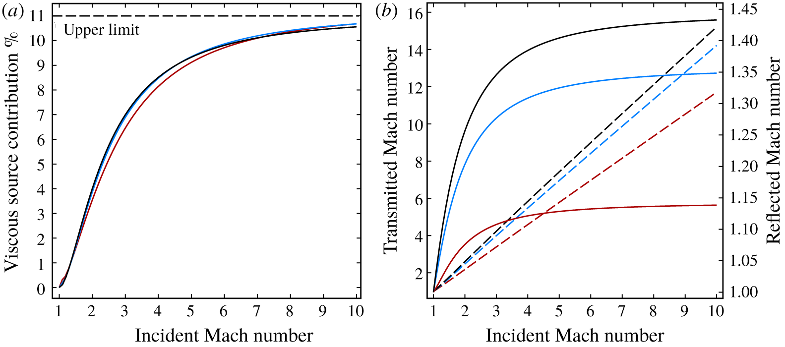
 $\unicode[STIX]{x1D702}$ (see figure 7b). However, the difference between the estimated and the exact solutions of
 $M_{r}$ has been proved to be quite small:
 $$\begin{eqnarray}M_{r}\approx 1-\frac{G(1)}{G^{\prime }(1)},\end{eqnarray}$$
where
 $$\begin{eqnarray}\left.\begin{array}{@{}c@{}}\displaystyle G(1)=T_{t}(M_{t0})-T_{i},\\ \displaystyle G^{\prime }(1)=T_{r}^{\prime }(1)T_{t}(M_{t0})T_{i}+T_{t}^{\prime }(M_{t0})M_{t}^{\prime }(1)+T_{r}^{\prime }(1)\end{array}\right\}\end{eqnarray}$$
and the values of  $T_{i},T_{t}(M_{t0}),M_{t}^{\prime }(1),T_{r}^{\prime }(1),T_{t}^{\prime }(M_{t0})$ are given by
 $$\begin{eqnarray}\left.\begin{array}{@{}l@{}}\displaystyle T_{i}=\frac{2\left({M_{i}}^{2}-1\right)\sqrt{{M_{1i}}^{2}-{M_{i}}^{2}}}{-2{M_{i}}^{3}+(\unicode[STIX]{x1D6FE}_{1}+1){M_{1i}}^{2}M_{i}+2M_{i}},\\ \displaystyle T_{t}(M_{t0})=\frac{2\left({M_{t0}}^{2}-1\right)\sqrt{{M_{1t}}^{2}-{M_{t0}}^{2}}}{-2{M_{t0}}^{3}+(\unicode[STIX]{x1D6FE}_{2}+1){M_{1t}}^{2}M_{t0}+2M_{t0}},\\ \displaystyle M_{t}^{\prime }(1)=\frac{C_{t1}}{\sqrt{C_{t1}+C_{t2}}},\\ \displaystyle T_{r}^{\prime }(1)=\frac{4\sqrt{{M_{1r}}^{2}-1}}{(\unicode[STIX]{x1D6FE}_{1}+1){M_{1r}}^{2}},\\ \displaystyle T_{t}^{\prime }(M_{t0})=\frac{-4{M_{t0}}^{4}+2{M_{1t}}^{2}{M_{t0}}^{2}+2{M_{1t}}^{2}}{{M_{t0}}^{2}[-2{M_{t0}}^{2}+(\unicode[STIX]{x1D6FE}_{2}+1){M_{1t}}^{2}+2]\sqrt{{M_{1t}}^{2}-{M_{t0}}^{2}}}\\ \displaystyle \qquad \qquad +\,\frac{8({M_{t0}}^{2}-1)\sqrt{{M_{1t}}^{2}-{M_{t0}}^{2}}}{[-2{M_{t0}}^{2}+(\unicode[STIX]{x1D6FE}_{2}+1){M_{1t}}^{2}+2]^{2}},\end{array}\right\}\end{eqnarray}$$
where
 $$\begin{eqnarray}M_{t0}=M_{t}(1)=\sqrt{C_{t1}+C_{t2}}.\end{eqnarray}$$
Consequently,  $M_{t}$ is obtained with (4.5).
We have provided the estimated solutions of  $M_{r}$ and
 $M_{t}$ as the elementary functions of the initial conditions (incident shock wave Mach number
 $M_{i}$, density ratio across the gas interface
 $\unicode[STIX]{x1D702}$, specific heat ratio of each gas
 $\unicode[STIX]{x1D6FE}_{1,2}$ and the initial angle of the gas interface
 $\unicode[STIX]{x1D6FC}_{0}$). Thus, the normalised circulation rate integral
 ${\mathcal{C}}_{s}^{\ast }$ and viscous source integral
 ${\mathcal{V}}_{s}^{\ast }$ for each shock are acquired by inserting
 $M_{i,r,t}$ into (3.7) and (3.34). Furthermore, the circulation rate and viscous source for an RMI problem with specific initial conditions are acquired with (4.1) and (4.2).
The normalised circulation rate  $\dot{\unicode[STIX]{x1D6E4}}^{\ast }$ and viscous source
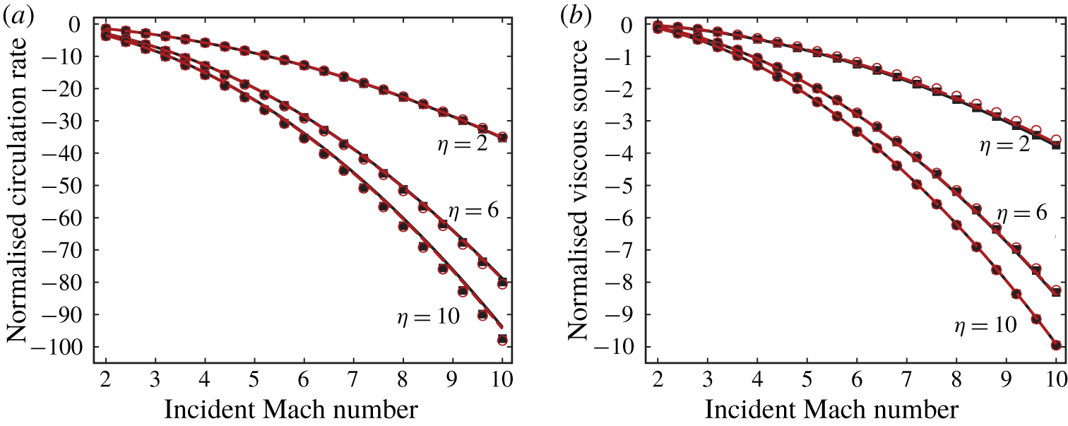
 $\dot{\unicode[STIX]{x1D6E4}}_{v}^{\ast }$ for RMI problems with various initial conditions are calculated and compared with the exact solutions obtained iteratively by shock polar analysis to verify the above-mentioned derived asymptotic approach of
 $M_{r}$ and
 $M_{t}$.
In shock polar analysis, the location of the intersections of the transmitted and reflected shock polars are determined numerically using the Newton iterative method. Multiple roots are always obtained, and the weakest root is known as the solution of physical significance (see Henderson Reference Henderson1966).
We tested the cases with  $M_{i}$ within the range of 2–10. Three different density ratios (
 $\unicode[STIX]{x1D702}=2,6,10$) and two initial angles of the gas interface (
 $\unicode[STIX]{x1D6FC}_{0}=45^{\circ },80^{\circ }$) are chosen. The gas pairs are all monatomic gases (
 $\unicode[STIX]{x1D6FE}_{1}=\unicode[STIX]{x1D6FE}_{2}=5/3,Pr_{1}=Pr_{2}=2/3$). The results are illustrated in figure 5. The difference between the predictions by two approaches does not monotonically vary with
 $\unicode[STIX]{x1D702}$, which can be understood by mathematical analysis from the governing equations of
 $\dot{\unicode[STIX]{x1D6E4}}^{\ast }$ and
 $\dot{\unicode[STIX]{x1D6E4}}_{v}^{\ast }$ as (4.1) and (4.2). In general, the results from the asymptotic approach show satisfactory agreement with the exact solutions given by the shock polar analysis within a wide range of initial conditions. This fact verifies the capability of the asymptotic approach in estimating the exact solutions.
Predictions of (a) the circulation rate and (b) the viscous source for RMI problems with different initial conditions. Symbols: ——, asymptotic approach of  $\unicode[STIX]{x1D6FC}_{0}=45^{\circ }$; - - - - -, asymptotic approach of
 $\unicode[STIX]{x1D6FC}_{0}=80^{\circ }$; ▪, shock polar analysis of
 $\unicode[STIX]{x1D6FC}_{0}=45^{\circ }$; ○, shock polar analysis of
 $\unicode[STIX]{x1D6FC}_{0}=80^{\circ }$.
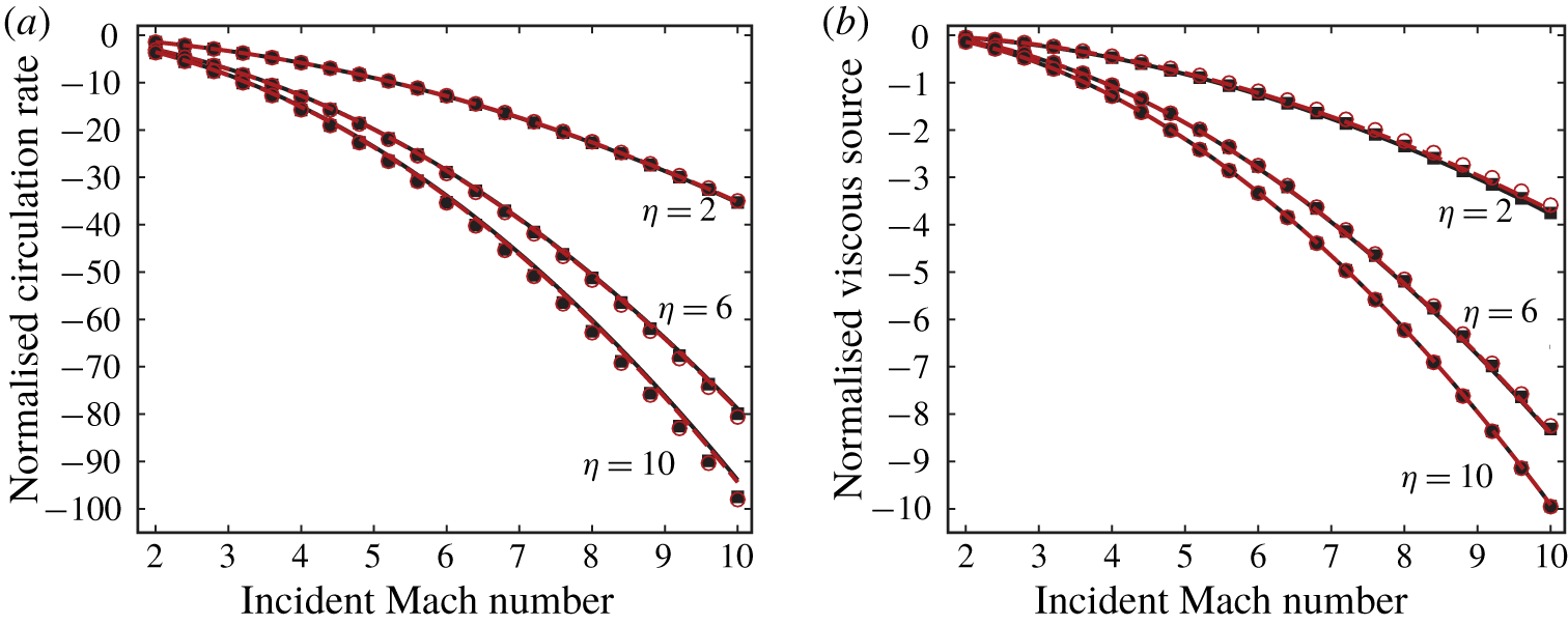
Another remarkable feature revealed by figure 5 is that the circulation rate and the viscous source show very low sensitivity to the initial angle of the gas interface (the red lines and symbols are very close to the black ones). In other words, the initial slope of the gas interface at the three-shock intersection slightly influence the circulation deposition process. The circulation rate and the viscous source at different moments are of approximately constant values when the shock wave interacts with a gas interface along which the initial slope is varied, such as a sinusoidal interface.
Therefore, we replace the local interface angle  $\unicode[STIX]{x1D6FC}_{0}$ in (4.8) by a global constant
 $\bar{\unicode[STIX]{x1D6FC}}=\arctan (h_{0}/w_{0})$, where
 $h_{0}$ and
 $w_{0}$ are defined by the initial geometry of the gas interface as demonstrated in figure 6. Notably,
 $\bar{\unicode[STIX]{x1D6FC}}$ is an approximation of the average slope of the gas interface. Its selection slightly influences the calculation of the circulation rate and viscous source. Furthermore, the circulation deposition of the SBI is theoretically predicted by simply considering
 $\bar{\unicode[STIX]{x1D6FC}}=45^{\circ }$.
Schematic of the RMI problem with curving initial gas interface.
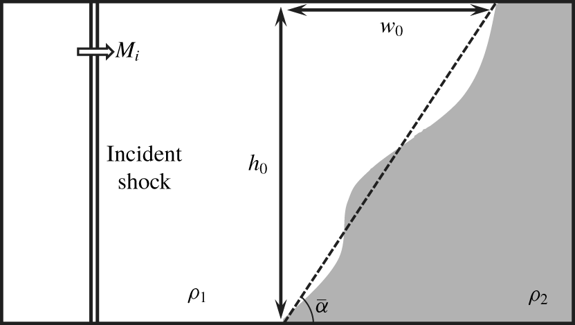
For an RMI problem with specific initial conditions, the entire predicting method of not only the growth rate of the circulation but also the contributions of different sources has been derived and verified comprehensively. This method consists of elementary functions of the initial conditions without the requirement for any numerical operations. Our model is based on the analysis about the properties inside a single shock wave. Accordingly, we abbreviate our model as the single-shock (SS) model.
4.2 Relative contribution of the viscous source
This study aims to reveal the contribution of viscosity to the circulation deposition in RMI. Thus, the level of contribution of the viscous source to the total circulation rate should be determined.
Here, we define the ratio of the viscous source to the circulation rate  ${\mathcal{R}}_{v}(=\dot{\unicode[STIX]{x1D6E4}}_{v}/\dot{\unicode[STIX]{x1D6E4}}\times 100\,\%)$ as the relative contribution of the viscous source. We predict
 ${\mathcal{R}}_{v}$ of the RMI problem with different initial conditions by using the SS model. The monatomic gas pairs (
 $\unicode[STIX]{x1D6FE}_{1}=\unicode[STIX]{x1D6FE}_{2}=5/3,Pr_{1}=Pr_{2}=2/3$) with varied incident Mach number and varied density ratio are investigated. The initial angle of the gas interface slightly influences the circulation deposition process. Thus, we keep it a constant as
 $\bar{\unicode[STIX]{x1D6FC}}=45^{\circ }$. The results are illustrated in figure 7(a).
Predictions of (a) the viscous source contribution  ${\mathcal{R}}_{v}$ (b) transmitted and reflected shock Mach numbers
 $M_{t}$ and
 $M_{r}$ for RMI problems with different
 $M_{i}$ and
 $\unicode[STIX]{x1D702}$ at
 $\bar{\unicode[STIX]{x1D6FC}}=45^{\circ }$. Red lines,
 $\unicode[STIX]{x1D702}=2$; blue lines,
 $\unicode[STIX]{x1D702}=6$; black lines,
 $\unicode[STIX]{x1D702}=10$. In panel (b), - - - - - -,
 $M_{r}$; ——,
 $M_{t}$.
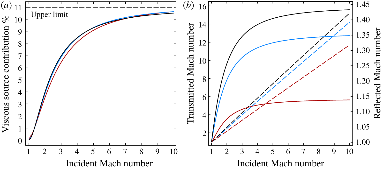
The relative contribution of the viscous source  ${\mathcal{R}}_{v}$ is mainly determined by the incident shock Mach number
 $M_{i}$. High
 $M_{i}$ leads to high
 ${\mathcal{R}}_{v}$. The density ratio
 $\unicode[STIX]{x1D702}$ has considerably less influence on
 ${\mathcal{R}}_{v}$.
Here, we explain the slight dependence of  ${\mathcal{R}}_{v}$ on
 $\unicode[STIX]{x1D702}$ qualitatively. We define
 ${\mathcal{R}}_{i,r,t}={\mathcal{C}}_{i,r,t}/\dot{\unicode[STIX]{x1D6E4}}$ as the relative contribution of each shock to the total circulation rate and
 ${\mathcal{R}}_{{\mathcal{V}}i,{\mathcal{V}}r,{\mathcal{V}}t}={\mathcal{V}}_{i,r,t}/{\mathcal{C}}_{i,r,t}$ as the ratio of viscous source integral of each shock. Accordingly,
 ${\mathcal{R}}_{v}$ can be expressed as
 $$\begin{eqnarray}{\mathcal{R}}_{v}={\mathcal{R}}_{i}{\mathcal{R}}_{{\mathcal{V}}i}+{\mathcal{R}}_{r}{\mathcal{R}}_{{\mathcal{V}}r}-{\mathcal{R}}_{t}{\mathcal{R}}_{{\mathcal{V}}t}.\end{eqnarray}$$
Six terms contribute to the variation in  ${\mathcal{R}}_{v}$ in (4.14);
 ${\mathcal{R}}_{i}$ and
 ${\mathcal{R}}_{{\mathcal{V}}i}$ depend mainly on the incident shock wave, and
 $\unicode[STIX]{x1D702}$ is assumed to slightly influence them. The four other terms depend on
 $M_{t}$ and
 $M_{r}$. The variations in
 $M_{t}$ and
 $M_{r}$ with
 $M_{i}$ for different
 $\unicode[STIX]{x1D702}$ at
 $\bar{\unicode[STIX]{x1D6FC}}=45^{\circ }$ are shown in figure 7(b).
With different  $\unicode[STIX]{x1D702}$ at the same
 $M_{i}$, a very slight variation in
 $M_{r}$ is observed. For instance, at
 $M_{i}=10$,
 $\unicode[STIX]{x1D702}$ varies from 2 to 10, whereas
 $M_{r}$ varies only from 1.14 to 1.43. Thus,
 $\unicode[STIX]{x1D702}$ slightly influences
 ${\mathcal{R}}_{r}$ and
 ${\mathcal{R}}_{{\mathcal{V}}r}$.
Here,  ${\mathcal{R}}_{t}$ is expressed as follows after inserting (4.1):
 $$\begin{eqnarray}{\mathcal{R}}_{t}=\frac{\unicode[STIX]{x1D702}^{-1}{\mathcal{C}}_{t}^{\ast }}{{\mathcal{C}}_{i}^{\ast }-\unicode[STIX]{x1D702}^{-1}{\mathcal{C}}_{t}^{\ast }+f_{i}{\mathcal{C}}_{r}^{\ast }}.\end{eqnarray}$$
High  $\unicode[STIX]{x1D702}$ leads to high
 $M_{t}$, whilst the increasing rate of
 $M_{t}$ is considerably lower than
 $\unicode[STIX]{x1D702}$. For instance, at
 $M_{i}=10$,
 $\unicode[STIX]{x1D702}$ increases five times (from 2 to 10), whereas
 $M_{t}$ increases only 1.3 times (from 11.7 to 15.2). This condition induces the decreasing trend of the term
 $\unicode[STIX]{x1D702}^{-1}{\mathcal{C}}_{t}^{\ast }$ with increasing
 $\unicode[STIX]{x1D702}$, which leads to the decreasing trend of
 ${\mathcal{R}}_{t}$. In the mean while high
 $M_{t}$ leads to high
 ${\mathcal{R}}_{{\mathcal{V}}t}$. The product of
 ${\mathcal{R}}_{t}$ and
 ${\mathcal{R}}_{{\mathcal{V}}t}$ is balanced nearly at a constant value with the variation in
 $\unicode[STIX]{x1D702}$. The slight dependence of the viscous source relative contribution
 ${\mathcal{R}}_{v}$ on the initial density ratio
 $\unicode[STIX]{x1D702}$ is explained mathematically.
We can also understand the small dependence of  ${\mathcal{R}}_{v}$ on
 $\unicode[STIX]{x1D702}$ physically. In § 6, it is proved that the viscous contribution to circulation deposition mainly comes from the large gradients of viscosity (
 $\unicode[STIX]{x1D735}\unicode[STIX]{x1D708}$ and
 $\unicode[STIX]{x1D735}\unicode[STIX]{x1D707}$) inside the strong shock waves. The shock strength determines the temperature gradient inside the shock and thus determines the viscosity gradient inside it. Thus, the viscous contribution should directly depend on the strength of shock waves in the flow field. The incident Mach number reflects the overall strength of the shock waves of an RMI problem. While the density ratio reflects the overall baroclinicity. It affects the magnitudes of circulation rate
 $\dot{\unicode[STIX]{x1D6E4}}$ and the viscous source
 $\dot{\unicode[STIX]{x1D6E4}}_{v}$. However, the relative contribution of the viscous source
 ${\mathcal{R}}_{v}=\dot{\unicode[STIX]{x1D6E4}}_{v}/\dot{\unicode[STIX]{x1D6E4}}$ is only slightly affected.
Another crucial feature of  ${\mathcal{R}}_{v}$ is its upper limit. Figure 7(a) shows that
 ${\mathcal{R}}_{v}$ tends to an upper limit, which is approximately 11 % (the dashed line in figure 7a), as incident Mach number increases. This condition can be understood in consideration of the limiting values of
 ${\mathcal{C}}_{s}^{\ast }$ and
 ${\mathcal{V}}_{s}^{\ast }$ for a single shock. From (3.7) and (3.34), we obtain
 $$\begin{eqnarray}\lim _{M_{s}\rightarrow \infty }{\mathcal{C}}_{s}^{\ast }\propto \lim _{M_{s}\rightarrow \infty }{\mathcal{V}}_{s}^{\ast }\propto {M_{s}}^{2}.\end{eqnarray}$$
This equation leads to the limiting value of  ${\mathcal{V}}_{s}^{\ast }/{\mathcal{C}}_{s}^{\ast }$ for a single shock and thus to the upper limit of
 ${\mathcal{R}}_{v}$.
5 Numerical results of the circulation deposition in RMI
5.1 Description and plan for present simulated cases
The RMI with different initial conditions is numerically simulated. The initial and boundary conditions of the cases are illustrated in figure 8.
Initially, the computational domain is divided into three parts by the incident shock and the gas interface, which are both discontinuities of flow quantities initially. The pre-shock temperature  $T_{0}=300~\text{K}$ and pressure
 $p_{0}=6.67~\text{N}~\text{m}^{-2}$ are the same as those in § 3.4. The post-shock temperature
 $T_{i}$, pressure
 $p_{i}$ and velocity
 $\boldsymbol{V}_{i}$ are calculated with the Rankine–Hugoniot shock relation. The gas on the right of the incident shock is initially stationary.
The initial position of the incident shock is  $x=0.001~\text{m}$. The starting location of the interaction is
 $x=0.06~\text{m}$. The region between
 $x=0.001~\text{m}$ and
 $x=0.06~\text{m}$ is for the full development of the incident shock from a flow discontinuity to a physically meaningful shock with finite thickness.
As for the boundary conditions, the left boundary is the inflow boundary with the post-shock values of the incident shock as flow quantities. The upper, lower and right boundaries are all symmetry boundaries.
Initial and boundary conditions of (a) cases 1–8; (b) case 9; (c) case 10; (d) case 11; and (e) case 12.
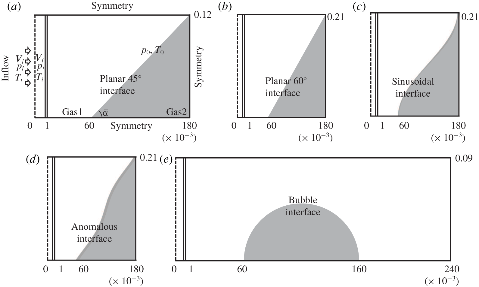
We numerically simulate 13 cases. The basic parameters of these cases are listed in table 2. Three basic parameters, namely, the incident shock strength  $M_{i}$, the initial density ratio
 $\unicode[STIX]{x1D702}$ and the initial shape of the gas interface, are considered.
Case 0 is the baseline. In this case, a strong shock ( $M_{i}=8$) interacts with the gas interface that divides argon and xenon. The initial density ratio is
 $\unicode[STIX]{x1D702}=3.29$. The initial shape of the gas interface is planar with
 $\bar{\unicode[STIX]{x1D6FC}}=45^{\circ }$. Cases 1–3 have the same parameters as case 0 except for the incident shock Mach number
 $M_{i}=2,4,6$. Cases 4–8 have different initial density ratios
 $\unicode[STIX]{x1D702}=9.99,6.51,4.15,2.10,1.57$ compared with case 0. Five different monatomic gases, namely, helium (He), neon (Ne), argon (Ar), krypton (Kr) and xenon (Xe), are used. Cases 0–8 have the same computational domain as
 $x\in (0,0.18)~\text{m}$ and
 $y\in (0,0.12)~\text{m}$.
As for cases 9–11, the initial shapes of the gas interface are different from case 0. Case 9 has a planar interface with  $\bar{\unicode[STIX]{x1D6FC}}=60^{\circ }$. Case 10 has a sinusoidal interface as
 $x=0.12-0.06\cos (\unicode[STIX]{x03C0}y/0.21)$. Case 11 has an anomalous interface as
 $x=0.12{-}0.06\cos (\unicode[STIX]{x03C0}y/0.21)+0.02\sin (2\unicode[STIX]{x03C0}y/0.21)$. Cases 9–11 have the same average angle of the initial gas interface as
 $\bar{\unicode[STIX]{x1D6FC}}=60^{\circ }$. Thus, they have the same computational domain as
 $x\in (0,0.18)~\text{m}$ and
 $y\in (0,0.21)~\text{m}$. Case 12 is the case of SBI. The computational domain is
 $x\in (0,0.24)~\text{m}$ and
 $y\in (0,0.09)~\text{m}$. The bubble interface is
 $(x-0.11)^{2}+y^{2}=0.05^{2}$ initially.
Overview of the simulated cases.
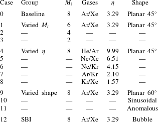
Here, we introduce the normalised time  $t^{\ast }=(tV_{s}-0.059)/w_{0}$, where
 $t$ is the physical time,
 $V_{s}$ is the moving velocity of the incident shock and
 $w_{0}$ is the width of the gas interface, as is demonstrated in figure 6 (
 $w_{0}$ equals the diameter of the initial bubble for the SBI case). At
 $t^{\ast }=0$, the shock reaches the gas interface. At
 $t^{\ast }=1$, the shock passes through the gas interface completely. The range of
 $t^{\ast }$ is
 $(-0.5,0.8)$ for cases 0–11, whereas
 $t^{\ast }\in (-0.6,1.73)$ for case 12.
In summary, the scope of the numerical simulations of this work covers the incident shock strength  $M_{s}$ from 2 to 8, density ratio
 $\unicode[STIX]{x1D702}$ from 1.57 to 9.99 and various shapes of the gas interface including the case of SBI.
5.2 Numerical method
The DSMC method is used in the numerical simulations of the above-mentioned cases. Given the large gradients of the flow parameters in the region of shock–interface interaction, the classical Navier–Stokes equation sets are unsuitable for describing the fluid dynamics within this region. The circulation deposition process occurs in this region. In appendix A, the necessity of using the DSMC method in our simulations is further illustrated by the local Knudsen number.
The molecular nature of the DSMC method enables it to simulate molecular, thermal and pressure diffusion physically. The near-equilibrium transport and non-equilibrium phenomena are considered inherently in the DSMC method. The RMI problem involves large gradients of flow parameters and multi-species diffusion, and the DSMC method has its apparent advantages in the simulation of this problem. In the region of interaction, the DSMC method can provide reliable simulations of the viscous stress  $\unicode[STIX]{x1D749}$ because it is based on the sampling of the molecular gas properties of each particle in a local cell but not the specific laws. This aspect is crucial for the accurate simulation of the viscous source. In recent years, molecular simulations of the RMI and RTI problems have been carried out in many investigations (Kadau et al. Reference Kadau, Germann, Hadjiconstantinou, Lomdahl, Dimonte, Holian and Alder2004; Zhakhovskii et al. Reference Zhakhovskii, Zybin, Abarzhi and Nishihara2006; Barber et al. Reference Barber, Kadau, Germann and Alder2007; Kadau et al. Reference Kadau, Rosenblatt, Barber, Germann, Huang, Carlès and Alder2007, Reference Kadau, Barber, Germann and Alder2008; Barber et al. Reference Barber, Kadau, Germann and Alder2008; Kadau et al. Reference Kadau, Barber, Germann, Holian and Alder2010; Abarzhi, Gauthier & Sreenivasan Reference Abarzhi, Gauthier and Sreenivasan2013; Livescu Reference Livescu2013; Gallis et al. Reference Gallis, Koehler, Torczynski and Plimpton2015, Reference Gallis, Koehler, Torczynski and Plimpton2016; Huang, Wang & Luo Reference Huang, Wang and Luo2018; Wu et al. Reference Wu, Huang, Ding, Wang and Luo2018; Zhang et al. Reference Zhang, Chen, Yu, He and Liu2019).
The majority of numerical RMI investigations are performed via Euler simulations. In the Euler simulations, the numerical viscosity exists because of the discrete approximation to the momentum advection term. Some numerical schemes also involve the artificial viscosity to obtain stable and smooth solutions across the discontinuities, such as shock waves. The numerical and artificial viscosities deviate from the physical viscosity and cannot provide accurate simulations of the viscous stress  $\unicode[STIX]{x1D749}$ inside the shock. The Euler solvers are inapplicable in simulations of the viscous source of circulation deposition in RMI. Even if a full Navier–Stokes solver is employed and sufficient cells are present inside the shock, the viscous stress inside the strong shock cannot be accurately simulated unless the linear Newtonian and Fourier law for
 $\unicode[STIX]{x1D749}$ and
 $\boldsymbol{q}$ are modified (see §§ 3.2 and 3.4).
However, if we only consider the circulation but not the sources of circulation deposition, then the Euler and Navier–Stokes solvers can provide reliable simulations. The  $(\unicode[STIX]{x1D70C},\unicode[STIX]{x1D70F}_{xx}-p)$ profile inside the shock remains unchanged as long as mass and momentum conservation across the shock is maintained (see § 3.1). Then the circulation rate remains unchanged according to (2.1). The Euler and Navier–Stokes solvers can accurately simulate circulation. However, these solvers are inapplicable in the simulation of the sources of circulation deposition and thus cannot reveal the real mechanism of circulation deposition in RMI. Hence, we use DSMC simulations here.
As for the DSMC simulations of the unsteady flow, the calculation is conducted for a large number of sampling times  $N_{s}$ independently. At every moment of output, the macroscopic gas properties
 $(\boldsymbol{V},p,T,\unicode[STIX]{x1D70C},\unicode[STIX]{x1D749})$ in each cell are determined by sampling the properties of computational particles in the cell for all the independent processes of computation. This procedure involves considerably more computational effort for unsteady DSMC simulations than steady DSMC simulations.
Our in-house parallel DSMC code for two-dimensional flow, which is mainly based on Bird (Reference Bird1994), is utilised in the simulations of cases 0–12. This code has been used in our recent studies (Ren, Liu & Jin Reference Ren, Liu and Jin2014; Chen, Zhang & Liu Reference Chen, Zhang and Liu2016; Zhang, Liu & Jin Reference Zhang, Liu and Jin2016; Liu et al. Reference Liu, Chen, Zhang and Liu2018; Chen, Zhang & Liu Reference Chen, Zhang and Liu2019; Liu et al. Reference Liu, Chen, Yu, Zhang and Liu2019; Zhang et al. Reference Zhang, Chen, Yu, He and Liu2019).
In our simulations, the standard subcell technique is utilised. Each cell is divided into five subcells in the  $x$ and
 $y$ directions, which indicates one sampling cell is divided into 25 collisional cells during the simulations, to decrease the mean collision separation of the particles. For all the simulated cases, the size of each collisional cell is
 $\unicode[STIX]{x0394}x_{c}=\unicode[STIX]{x0394}y_{c}=6\times 10^{-5}~\text{m}$.
The time steps  $\unicode[STIX]{x0394}t$ for different cases differ. The time step for case 0 is
 $\unicode[STIX]{x0394}t=3.75\times 10^{-9}~\text{s}$. For cases 1–12, the displacement of the incident shock at every time step
 $(V_{s}\unicode[STIX]{x0394}t)$ has the same approximate value as case 0. Specifically, case 1 has
 $\unicode[STIX]{x0394}t=5\times 10^{-9}~\text{s}$, case 2 has
 $\unicode[STIX]{x0394}t=7.5\times 10^{-9}~\text{s}$, case 3 has
 $\unicode[STIX]{x0394}t=1.5\times 10^{-8}~\text{s}$, case 4 has
 $\unicode[STIX]{x0394}t=1.19\times 10^{-9}~\text{s}$, cases 5 and 6 have
 $\unicode[STIX]{x0394}t=2.5\times 10^{-9}~\text{s}$, case 7 has
 $\unicode[STIX]{x0394}t=3.75\times 10^{-9}~\text{s}$, case 8 has
 $\unicode[STIX]{x0394}t=5.43\times 10^{-9}~\text{s}$ and cases 9–12 have
 $\unicode[STIX]{x0394}t=3.75\times 10^{-9}~\text{s}$.
The time of sampling is  $N_{s}=1600$ for all the cases. The initial number of computational particles per sampling cell in the lowest density region (between the shock wave and the gas interface) is
 $N_{p0}=24$. In the other regions,
 $N_{p0}$ is proportional to the local number density of real particles. A total of 80 equispaced output files are used for cases 0–11 and 120 for case 12. The validation, verification and numerical accuracy of our simulations are comprehensively demonstrated in appendix A.
5.3 Visualisation of the flow field
In this subsection, the interacting process of the shock wave and the gas interface and the circulation deposition process are visualised and investigated. For instance, three cases, namely, case 0 (planar interface), case 10 (sinusoidal interface) and case 12 (bubble interface), are considered. These cases are commonly investigated configurations.
Density (top) and vorticity (bottom) fields and the theoretical predicted flow configurations of case 0 at (a) the beginning ( $t^{\ast }=0.65$) and (b) the end (
 $t^{\ast }=0.8$) of the considered time period.
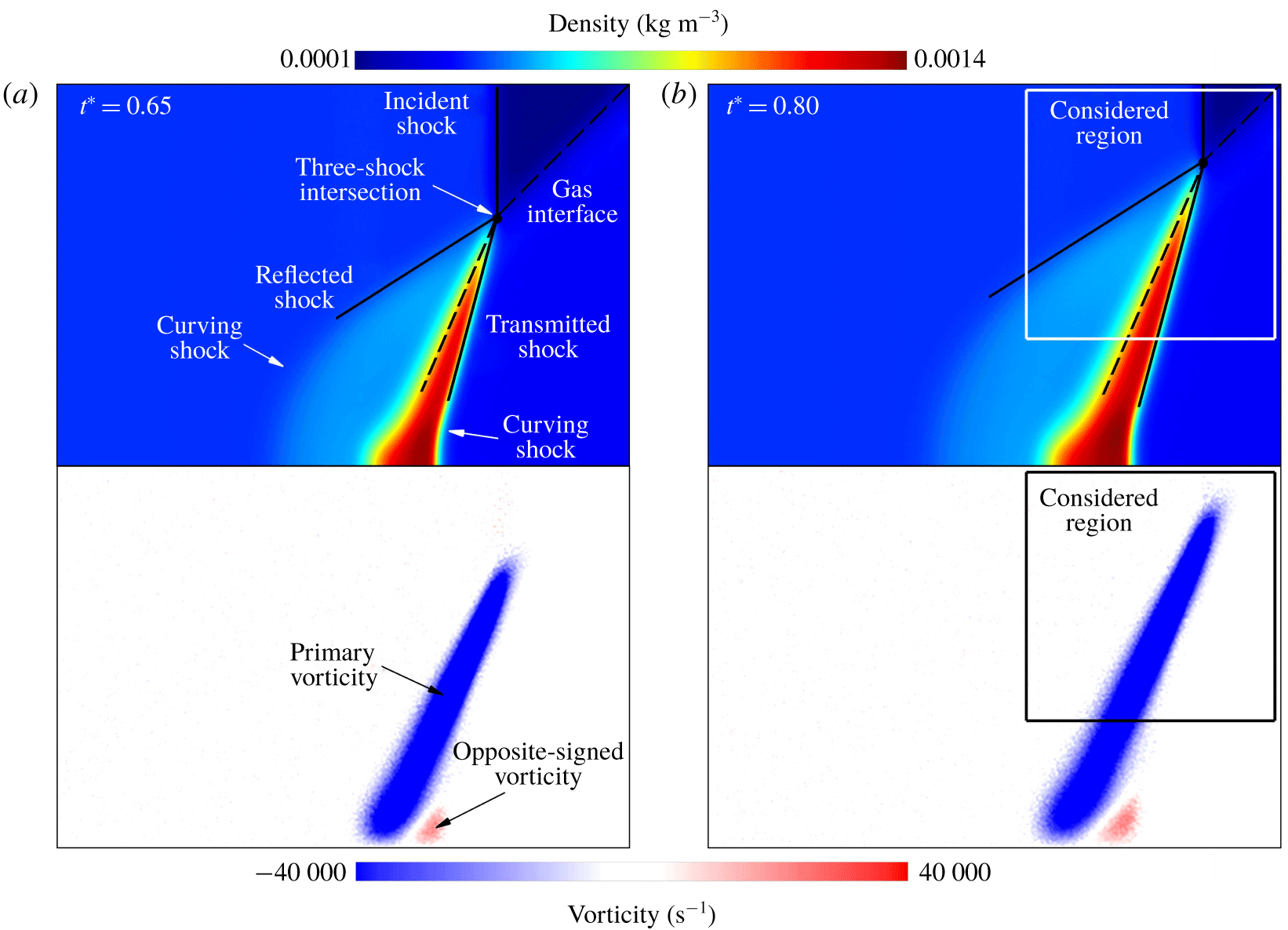
The density  $\unicode[STIX]{x1D70C}$ and vorticity
 $\unicode[STIX]{x1D714}=\unicode[STIX]{x1D735}\times \boldsymbol{V}$ fields of case 0 at two specific moments (
 $t^{\ast }=0.65$ and
 $t^{\ast }=0.8$) are visualised in figure 9. The local vorticity is proportional to the local velocity gradient, which is disturbed by the noise for DSMC results. We use an averaging method to reduce the noise of the local vorticity to provide a better visualisation of the vorticity field. At every cell, an averaged vorticity is calculated, which is the average of the vorticity in eight surrounding cells and itself. Figure 9 shows the vorticity fields with reduced noise.
The theoretical predicted flow configurations are also illustrated by solid and dashed lines. The angle of the reflected and transmitted shocks and the post-shock gas interface are theoretically obtained as long as the shock strengths ( $M_{r}$ and
 $M_{t}$) are known, which are predicted by the aforementioned derived asymptotic approach. The density contours in figure 9 demonstrate that the predicted flow configurations coincide with the numerical simulated results quite well in the vicinity of the three-shock intersections.
When the shock waves pass the interface, the misalignment of the density and pressure gradients is the major source of the vorticity deposition along the shocked gas interface, namely, the baroclinic source. Theoretically, negative vorticity generation occurs along the gas interface, which coincides with the blue region in the vorticity fields in figure 9.
Figure 9 shows that opposite-signed vorticity deposition is generated near the lower boundary and behind the transmitted shock in addition to the primary vorticity generation caused by the shock–interface interaction. The reflected and transmitted shocks curve in the region near the lower boundary due to the symmetric boundary condition at the lower boundary (see figure 9). These curving shocks generate the opposite-signed vorticity behind them (see Kevlahan Reference Kevlahan1997; Zabusky Reference Zabusky1999), which is beyond the scope of this investigation.
In some previous studies based on Navier–Stokes solvers, the negative and positive magnitudes of vorticity are separately integrated to obtain the negative and positive circulations (see Yang et al. Reference Yang, Chern, Zabusky, Samtaney and Hawley1992; Kotelnikov et al. Reference Kotelnikov, Ray and Zabusky2000; Peng et al. Reference Peng, Zabusky and Zhang2003; Lee et al. Reference Lee, Peng and Zabusky2006). For DSMC results, the noise of the simulated results makes this treatment inapplicable. Thus, a proper integral boundary should be chosen when calculating the magnitude of the circulation deposition.
In our numerical simulations, the computational domain and the initial interface location are the same in cases 0–8. Thus, the considered regions for them are chosen as  $x=0.1,0.178~\text{m}$ for the left and right boundaries and
 $y=0.04,0.118~\text{m}$ for the lower and upper boundaries, which are illustrated as boxes in figure 9. For cases 9–11, the lower and upper boundaries are
 $y=0.07,0.208~\text{m}$ and the left and right ones remain the same as cases 0–8. Case 12 is the case of the SBI; the whole computational domain is taken as the considered region as in previous studies (Niederhaus et al. Reference Niederhaus, Greenough, Oakley, Ranjan, Anderson and Bonazza2008). The next subsection proves that the considered results are less sensitive to the region boundaries.
Similarly, figure 10 exhibits the density and vorticity fields of case 10 (sinusoidal interface) at  $t^{\ast }=0.8$. The theoretically predicted flow configurations are shown as solid and dashed lines. We use the local interface angle
 $\unicode[STIX]{x1D6FC}_{0}$ at the theoretical predicted three-shock intersection to predict the angles of the shocks and post-shock interface. This time, the theoretically predicted angles of the shocks and post-shock interface slightly deviate from the numerically simulated results.
The local interface angle in figure 10 is  $\unicode[STIX]{x1D6FC}_{0}\approx 54^{\circ }$. In figure 9, the case of
 $\unicode[STIX]{x1D6FC}_{0}=45^{\circ }$ is demonstrated, and the theoretically predicted shocks and interface efficiently coincide with the numerically simulated ones. We also obtained satisfactory agreement between the theoretical and numerical flow configurations for case 9 (not shown), which is the case of
 $\unicode[STIX]{x1D6FC}_{0}=60^{\circ }$. These two cases are planar interface cases. It is reasonable to believe that the theoretical and numerical flow configurations will coincide with each other for the planar interface case with
 $\unicode[STIX]{x1D6FC}_{0}=54^{\circ }$.
The deviation of the theoretically predicted flow configuration from the numerically simulated one observed in figure 10 is attributed to the high local curvature of the interface. We consider the relative magnitude of the local curvature  $\unicode[STIX]{x1D705}$ of the interface and the shock wave thickness
 $\unicode[STIX]{x1D6FF}_{s}$ in RMI. If the local curvature of the interface is relatively low (
 $\unicode[STIX]{x1D705}\unicode[STIX]{x1D6FF}_{s}\ll 1$), then the variation of the local interface angle
 $\unicode[STIX]{x1D6FC}_{0}$ is rather small in the vicinity of the three-shock intersection. The interaction tends to the case of shock–planar interface interaction. This is the condition of most practical RMI problems. Otherwise, the local interface angle
 $\unicode[STIX]{x1D6FC}_{0}$ slightly varies in the region of interaction, which is the condition of case 10 here. The use of the local interface angle at the theoretically predicted three-shock intersection will lead to a slight deviation of the predicted flow configuration from the real one (numerically simulated result).
It has been demonstrated in § 4.1 that  $\unicode[STIX]{x1D6FC}_{0}$ scarcely affects the prediction of the circulation deposition process. Thus, the above-observed deviation of the predicted flow configuration, mainly induced by the imprecise
 $\unicode[STIX]{x1D6FC}_{0}$, scarcely affects our theoretical prediction of the circulation deposition process.
In the vorticity field of case 10, the vorticity significantly deposits on the shocked interface as a sinusoidal shape. This occurrence has also been observed in previous studies (Zabusky Reference Zabusky1999). In this case, no significant opposite-signed vorticity deposition exists as in case 0. The curvature of the transmitted shock in this case is much lower than that in case 0, which is evident in figures 9 and 10.
Density (left) and vorticity (right) fields and the theoretical predicted flow configurations of case 10 at the end ( $t^{\ast }=0.8$) of the considered time period.
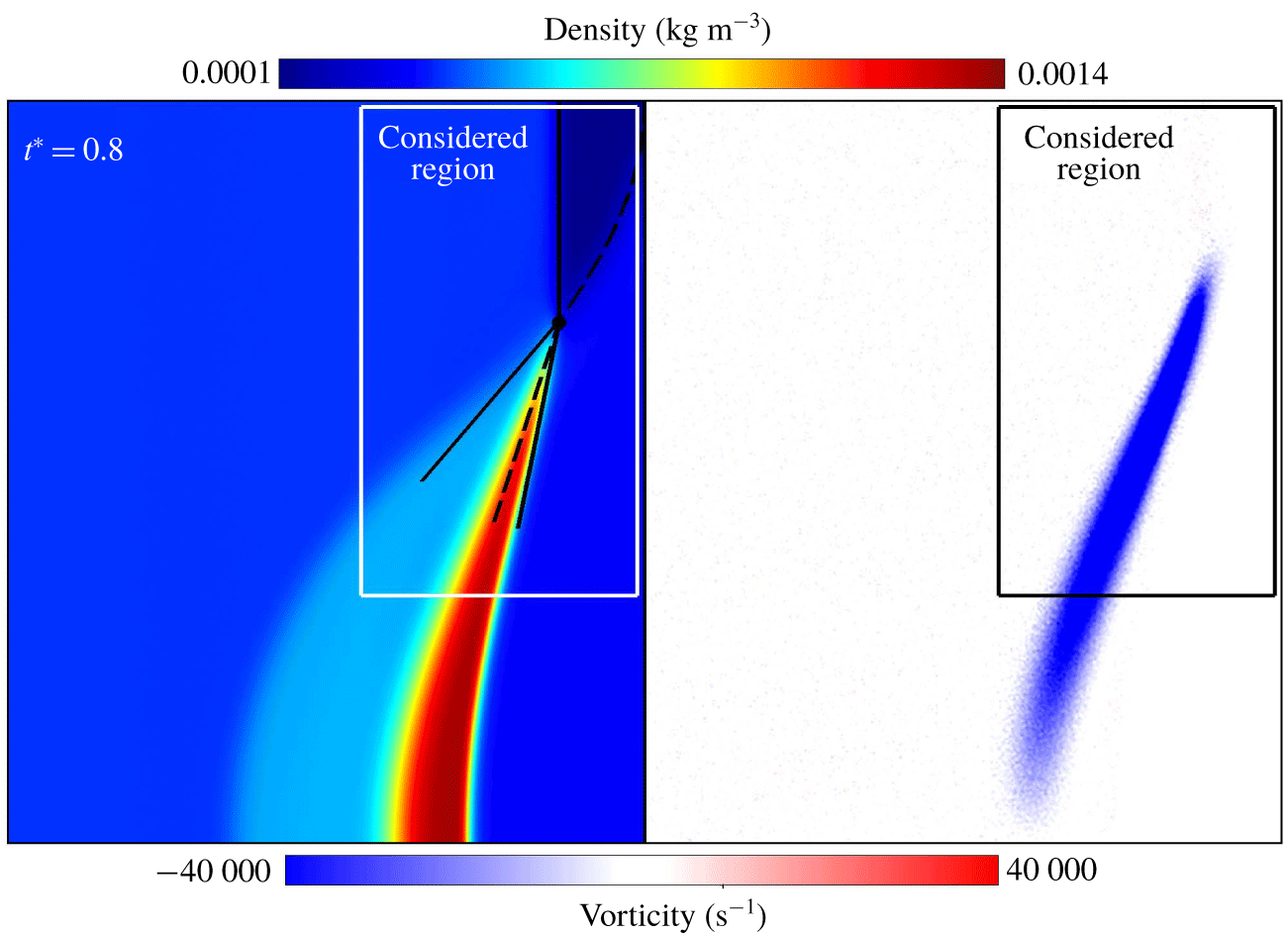
Figure 11 demonstrates the density and vorticity fields in the bubble vicinity of the SBI case. Three specific moments ( $t^{\ast }=0.2,0.5$ and
 $1.2$) are shown. The vorticity fields are mirrored by the
 $y=0$ plane for clear comparisons with the density fields. The gas interfaces are shown by the isolines of the mass fraction of argon
 $Y_{Ar}=0.1$ and
 $0.9$ in the vorticity fields.
During the early stage of the interaction, as shown in figure 11(a), the flow configuration is similar to those in figures 9 and 10. The incident, transmitted and reflected shocks meet at a single point on the interface. The regular refraction occurs. Here, we do not show the theoretically predicted flow configurations on the basis of local analysis because the local curvature of the interface is even higher than that in case 10. The deviation of the predicted flow configuration from the simulated one will be significant. However, this deviation scarcely affects the prediction of the circulation deposition process, which has been explained above. At  $t^{\ast }=0.5$, the three-shock intersection is at the top of the bubble, i.e.
 $\unicode[STIX]{x1D6FC}_{0}=0^{\circ }$, as shown in figure 11(b). The irregular refraction occurs. The flow configuration of irregular refraction is quite complex, and we do not discuss that in detail. In the time period of
 $t^{\ast }<0.5$, the local interface angle
 $\unicode[STIX]{x1D6FC}_{0}$ continuously varies from
 $90^{\circ }$ to
 $0^{\circ }$. The incident shock remains planar, and the reflected shock does not contact with the upper boundary. The vorticity is deposited inside the mixing region of the interface.
At  $t^{\ast }=1.2$, the incident shock moves over the top of the bubble and curves back to meet the interface, as shown in figure 11(c). The bubble is significantly compressed by the shocks. The gas interface is highly diffused, and the mixing region is rather thick. The vorticity generation can be distinguished as three different parts, as illustrated in figure 11(c). The first part is the primary vorticity deposition inside the mixing region induced by the interaction. The second part is the opposite-signed vorticity deposition inside the bubble induced by the highly curved transmitted shock. The internally reflected rarefaction waves (Niederhaus et al. Reference Niederhaus, Greenough, Oakley, Ranjan, Anderson and Bonazza2008; Ranjan et al. Reference Ranjan, Oakley and Bonazza2011) exist in that region and affect the vorticity evolution. The third part is the additional vorticity deposition induced by the curved incident shock.
The flow configurations significantly vary during the interaction from regular ( $t^{\ast }=0.2$) to irregular (
 $t^{\ast }=0.5$) refraction and finally to a rather complex flow configuration with a highly deformed bubble (
 $t^{\ast }=1.2$). The following subsection demonstrates that the circulation rate and sources remain nearly constant during the whole time period in figure 11 (
 $0.2<t^{\ast }<1.2$). Similar statements have been claimed by Samtaney & Zabusky (Reference Samtaney and Zabusky1994) when they extended the SZ model to the SBI case.
Density (top) and vorticity (bottom) fields of case 12 at (a) the beginning ( $t^{\ast }=0.2$), (b) middle (
 $t^{\ast }=0.5$) and (c) end (
 $t^{\ast }=1.2$) of the considered time period. The gas interfaces (
 $Y_{Ar}=0.1,0.9$) are shown as solid lines in the vorticity fields.
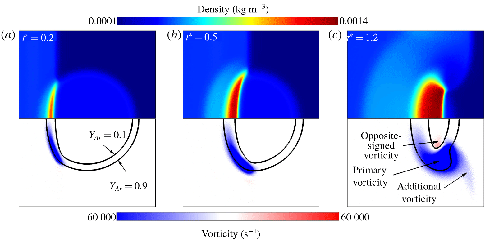
5.4 Circulation rate and sources
The circulation deposition and its sources for the numerical simulated results are examined. For the calculation of the circulation at a specific moment, the surface integral of the vorticity is carried out, that is,  $\unicode[STIX]{x1D6E4}=\int \unicode[STIX]{x1D714}\,\text{d}A$. The above-mentioned noise reducing method for the vorticity field does not change the result of the surface integral of vorticity. Thus it is not used in the calculation of circulation.
With the circulation at every moment, the normalised circulation rate  $\dot{\unicode[STIX]{x1D6E4}}^{\ast }=(\unicode[STIX]{x1D70C}_{01}/p_{0})(\text{d}\unicode[STIX]{x1D6E4}/\text{d}t)$ is easily obtained by carrying out the numerical differentiation of the circulation at every moment.
As for the normalised baroclinic source  $\dot{\unicode[STIX]{x1D6E4}}_{b}^{\ast }$ and viscous source
 $\dot{\unicode[STIX]{x1D6E4}}_{v}^{\ast }$, Green’s theorem is used and expressed as (5.1), where the local baroclinic source
 $\dot{\unicode[STIX]{x1D714}}_{b}$ and the local viscous source
 $\dot{\unicode[STIX]{x1D714}}_{v}$ are introduced.
 $$\begin{eqnarray}\left.\begin{array}{@{}c@{}}\displaystyle \dot{\unicode[STIX]{x1D6E4}}_{b}^{\ast }=-\frac{\unicode[STIX]{x1D70C}_{01}}{p_{0}}\oint _{C}\unicode[STIX]{x1D70C}^{-1}\unicode[STIX]{x1D735}p\boldsymbol{\cdot }\text{d}\boldsymbol{s}=-\frac{\unicode[STIX]{x1D70C}_{01}}{p_{0}}\int _{A}\unicode[STIX]{x1D735}\times (\unicode[STIX]{x1D70C}^{-1}\unicode[STIX]{x1D735}p)\,\text{d}A=\frac{\unicode[STIX]{x1D70C}_{01}}{p_{0}}\int _{A}\dot{\unicode[STIX]{x1D714}}_{b}\,\text{d}A,\\ \displaystyle \dot{\unicode[STIX]{x1D6E4}}_{v}^{\ast }=\frac{\unicode[STIX]{x1D70C}_{01}}{p_{0}}\oint _{C}\unicode[STIX]{x1D70C}^{-1}\unicode[STIX]{x1D735}\boldsymbol{\cdot }\unicode[STIX]{x1D749}\boldsymbol{\cdot }\text{d}\boldsymbol{s}=\frac{\unicode[STIX]{x1D70C}_{01}}{p_{0}}\int _{A}\unicode[STIX]{x1D735}\times (\unicode[STIX]{x1D70C}^{-1}\unicode[STIX]{x1D735}\boldsymbol{\cdot }\unicode[STIX]{x1D749})\,\text{d}A=\frac{\unicode[STIX]{x1D70C}_{01}}{p_{0}}\int _{A}\dot{\unicode[STIX]{x1D714}}_{v}\,\text{d}A.\end{array}\right\}\end{eqnarray}$$
The basis of our theoretical predictions of the circulation deposition process is (1.1). The circulation boundary is a closed material curve, and the transport of vorticity across the boundary is inherently absent. In our numerical results of the circulation deposition, the circulation boundary (the considered region) is a fixed one because it is difficult to exactly determine a material curve from the numerical results. A circulation variation occurs due to the transport of vorticity across the boundary as
 $$\begin{eqnarray}\dot{\unicode[STIX]{x1D6E4}}_{t}^{\ast }=-\frac{\unicode[STIX]{x1D70C}_{01}}{p_{0}}\oint _{C}(\boldsymbol{V}\boldsymbol{\cdot }\unicode[STIX]{x1D735})\boldsymbol{V}\boldsymbol{\cdot }\text{d}\boldsymbol{s}=-\frac{\unicode[STIX]{x1D70C}_{01}}{p_{0}}\int _{A}\unicode[STIX]{x1D735}\boldsymbol{\cdot }(\unicode[STIX]{x1D714}\boldsymbol{V})\,\text{d}A.\end{eqnarray}$$
The surface integral is carried out in the considered region described in the last subsection. The numerical differentiations are all calculated with the method of second-order centre difference. The baseline (case 0) is taken as an example to show the evolution of the circulation, the normalised circulation rate, the sources and the circulation transport, as shown in figure 12(a).
In the time period before  $t^{\ast }=0$, the incident shock develops from a discontinuity to a physically meaningful shock with finite thickness. At
 $t^{\ast }=0$, the incident shock reaches the gas interface and the interaction starts. While at that time, the shock waves have not entered the considered region yet. As a result, no circulation deposition is observed in figure 12(a). From
 $t^{\ast }\approx 0.3$, the shock front enters the considered region and the circulation deposition process in that region starts.
In figure 12(a), the circulation increases linearly when the shocks get into the considered region entirely ( $t^{\ast }\gtrsim 0.4$). Therefore, the circulation deposition process can be treated as a quasi-steady process, and the circulation rate and the sources should have constant values. The numerical results in figure 12(a) confirm this statement.
Here, we choose a specific time period and use the average values of  $\dot{\unicode[STIX]{x1D6E4}}_{b}^{\ast },\dot{\unicode[STIX]{x1D6E4}}_{v}^{\ast }$ and
 $\dot{\unicode[STIX]{x1D6E4}}_{t}^{\ast }$ in it as the numerical results of the normalised baroclinic and viscous sources
 $\dot{\unicode[STIX]{x1D6E4}}_{b}^{\ast \ast },\dot{\unicode[STIX]{x1D6E4}}_{v}^{\ast \ast }$ and the normalised circulation transport
 $\dot{\unicode[STIX]{x1D6E4}}_{t}^{\ast \ast }$ for specific RMI problems with different initial conditions. The circulation rates
 $\dot{\unicode[STIX]{x1D6E4}}^{\ast \ast }$ for specific cases are obtained from the slope of the linear fitted circulation in the considered time period.
In the considered time period, the circulation deposition process should be quasi-steady, and  $\dot{\unicode[STIX]{x1D6E4}}_{b}^{\ast }$ and
 $\dot{\unicode[STIX]{x1D6E4}}_{v}^{\ast }$ should be nearly constant. During the early time period of the interaction (
 $t^{\ast }\ll 1$), the region between the transmitted shock and the shocked gas interface is too small. In this region, the flow quantities are highly non-uniform and seriously deviate from our theoretically predicted values. In the late time period of the interaction (
 $1-t^{\ast }\ll 1$), the incident shock is affected by the right boundary. For cases 0–11, we choose
 $t^{\ast }\in (0.65,0.8)$ as the considered time period. The flow and vorticity fields of case 0 at the beginning and end moments are visualised in figure 9. The values of the circulation rate and the sources are approximately constant values in the time period of consideration, as shown as the blue zone in figure 12(a).
The theoretically predicted values of the circulation rate and the sources by our SS model are also shown by red dashed lines in the considered time period. They coincide with numerically simulated results quite well.
The normalised circulation transport across the region boundary  $\dot{\unicode[STIX]{x1D6E4}}_{t}^{\ast }$ is much lower in the considered time period compared with the circulation rate. The values of
 $\dot{\unicode[STIX]{x1D6E4}}^{\ast \ast }$ and
 $\dot{\unicode[STIX]{x1D6E4}}_{t}^{\ast \ast }$ are 0.07 and
 $-36.36$, respectively. Thus, the numerical results of the circulation deposition obtained by using a fixed curve or a material curve as the circulation boundary are quite close to each other.
Evolution of the circulation, the circulation rate, the baroclinic and viscous source for (a) case 0 (b) case 12. Symbols: ——, circulation; ●, normalised circulation rate; ▵, normalised baroclinic source; ▫, normalised viscous source;  $+$, normalised circulation transport; - - - - - -, theoretical predictions of the SS model.
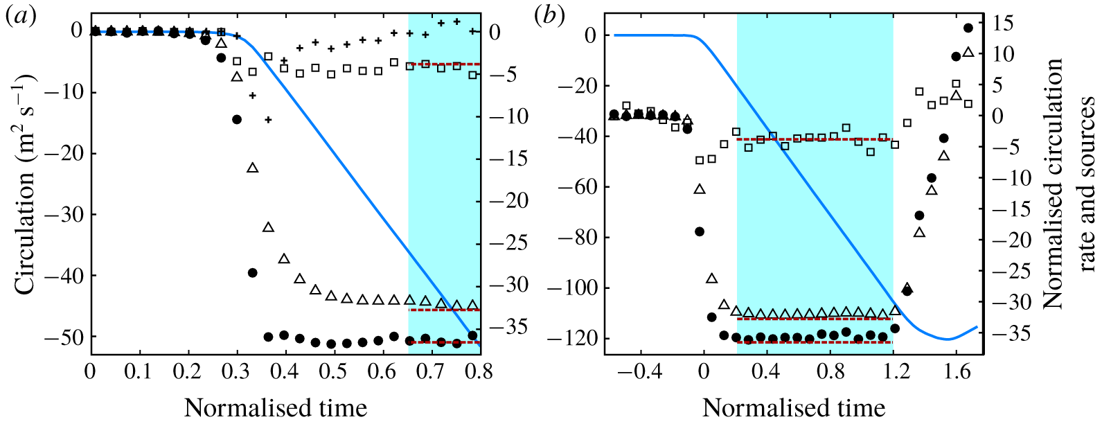
In our simulations, the sensitivities of the numerical results  $\dot{\unicode[STIX]{x1D6E4}}^{\ast \ast }$,
 $\dot{\unicode[STIX]{x1D6E4}}_{b}^{\ast \ast }$ and
 $\dot{\unicode[STIX]{x1D6E4}}_{v}^{\ast \ast }$ to the selections of the considered region and time period are low. Here, we use bigger and smaller considered regions as well as longer and shorter considered time periods compared to the original ones to prove this situation. Case 0 is taken as an example, and table 3 demonstrates the results. The variations in the circulation rate and the sources are small for different selections of the considered regions and time periods.
Sensitivity of the numerical results to the considered region size and time period.
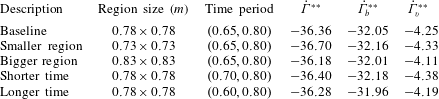
Case 12 is the case of SBI, and the circulation deposition and evolution are demonstrated in figure 12(b). The considered region is the whole computational domain. No circulation transport exists ( $\dot{\unicode[STIX]{x1D6E4}}_{t}^{\ast }=0$) due to
 $\unicode[STIX]{x1D714}=0$ along the circulation boundary. During a long period (
 $t^{\ast }$ from approximately 0.2 to 1.2), the circulation increases linearly. For the SBI problem, the local angle of the initial gas interface varies continuously from
 $90^{\circ }$ to
 $-90^{\circ }$, but the circulation rate and sources remain at constant values in most of the interacting time periods. The values are very close to our theoretically predicted values (red dashed lines). This closeness confirms the applicability of our SS model in the SBI problem. Here, we use average values of the circulation rate and the sources in the range of
 $t^{\ast }\in (0.2,1.2)$ as the primary circulation deposition results for case 12, as shown as the blue region in figure 12(b). The flow fields at the beginning and end moments of the considered time period are demonstrated in figure 11(a,c). After this period, the circulation drops due to the deposition of opposite-signed vorticity by reflected shocks (see Zabusky & Zeng Reference Zabusky and Zeng1998; Niederhaus et al. Reference Niederhaus, Greenough, Oakley, Ranjan, Anderson and Bonazza2008), which is beyond the scope of this investigation.
5.5 Circulation deposition for different RMI cases
The circulation deposition processes for the cases with different initial conditions are observed and investigated. The numerical results are calculated in the time and space region described above, including the circulation rate  $\dot{\unicode[STIX]{x1D6E4}}^{\ast \ast }$, the baroclinic source
 $\dot{\unicode[STIX]{x1D6E4}}_{b}^{\ast \ast }$, the viscous source
 $\dot{\unicode[STIX]{x1D6E4}}_{v}^{\ast \ast }$ and relative contribution of the viscous source
 ${\mathcal{R}}_{v}$. In the meantime, the theoretical predictions of these parameters by our SS model are also provided, noted with the subscript ‘SS’.
The predictions of the circulation rate by the popular circulation model, that is, the SZ model, are also provided to compare with our SS model. The first-order SZ model provides the circulation deposition per unit length  $l$ of the original gas interface as
 $$\begin{eqnarray}\frac{\text{d}\unicode[STIX]{x1D6E4}}{\text{d}l}=\frac{2\sqrt{\unicode[STIX]{x1D6FE}_{c}}}{\unicode[STIX]{x1D6FE}_{c}+1}(1-\unicode[STIX]{x1D702}^{-1/2})(1+{M_{i}}^{-1}+2{M_{i}}^{-2})(M_{i}-1)\cos \unicode[STIX]{x1D6FC}_{0},\end{eqnarray}$$
where  $\unicode[STIX]{x1D6FE}_{c}=(\unicode[STIX]{x1D6FE}_{1}+\unicode[STIX]{x1D6FE}_{2})/2$ is a characteristic specific heat ratio. Then, the time rate of the circulation given by the first-order SZ model can be expressed as
 $$\begin{eqnarray}\dot{\unicode[STIX]{x1D6E4}}_{SZ1}^{\ast }=\frac{\text{d}\unicode[STIX]{x1D6E4}}{\text{d}l}\frac{\text{d}l}{\text{d}t}=\frac{2\sqrt{\unicode[STIX]{x1D6FE}_{c}\unicode[STIX]{x1D6FE}_{1}}}{\unicode[STIX]{x1D6FE}_{c}+1}(1-\unicode[STIX]{x1D702}^{-1/2})M_{i}(1+{M_{i}}^{-1}+2{M_{i}}^{-2})(M_{i}-1).\end{eqnarray}$$
Equation (5.3) is the proposed scaling law of the circulation derived by the asymptotic method in the SZ model. This model is a first-order estimation of the exact solution. A third-order estimation and an exact solution of the circulation are also provided by Samtaney & Zabusky (Reference Samtaney and Zabusky1994). These predictions require numerical treatments to solve the flow direction and pressure across the shocked gas interface. Here, we compare the first-order SZ model and our SS model because they are all first-order estimations and have the same complexity of calculation (neither of them requires numerical treatment).
For the problem of the SBI, the 1-D model (Niederhaus et al. Reference Niederhaus, Greenough, Oakley, Ranjan, Anderson and Bonazza2008) can also predict the circulation rate and shows best agreements with the numerical simulated results amongst the predicting models in their study. Unfortunately, their model relies on an empirical model of the on-axis gas velocity, shown as equation (6.17) in Niederhaus et al. (Reference Niederhaus, Greenough, Oakley, Ranjan, Anderson and Bonazza2008), which is obtained by fitting the numerically simulated results. Their model solves the strength of the transmitted and reflected shocks iteratively, requiring numerical treatment. Thus, we do not compare our SS model with the 1-D model in this study.
The results for cases 0–12 are listed in table 4. The circulation rate and the sources are all normalised with unit pre-shock pressure and density.
Results for the circulation deposition and sources for cases 0–12.
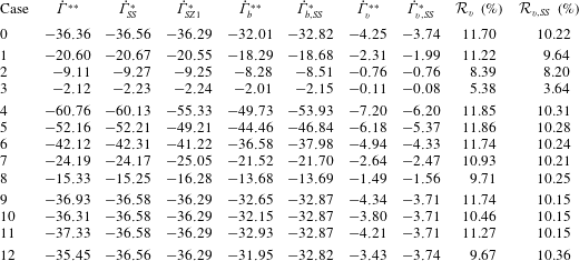
As for the circulation rate, the predictions by the SS and SZ models show satisfying agreement with the numerical results for nearly all cases. The relative errors of the predictions by the two models are quite small, verifying the capabilities of both models in a large range of initial conditions. Among the cases, the prediction of case 4 by the first-order SZ model deviates from the numerical result most (the relative error is 8.9 %). Case 4 is the case with the highest incident Mach number and density ratio. If the third-order or the exact solution of the SZ model is employed, much better agreement can be obtained. The exact solution of the SZ model accurately solves the physical conditions (equal pressure and flow direction across the post-shock interface), and integrates the velocity field to obtain the circulation. This prediction is based on the conservation laws of the fluid and does not introduce particular assumptions or simplifications. Thus, it can precisely predict the circulation (consider only the regular refraction).
In the circulation rate predictions, our SS model, which does not require numerical treatment, achieves the same level of precision as the exact solution of the SZ model. The two models are different in the solving of post-shock flow conditions. Instead of the shock polar analysis, our model uses the asymptotic series in  $M_{r}$, which is close to 1 in the whole range of initial parameters. The predictions of circulation by two models are equivalent in the physical basis, as shown as (1.1) and (1.3).
In the group of varied interface shapes (cases 9–12), the properties of the SS and first-order SZ models are similar. The circulation rate is independent of the interface shape, as shown in (5.4). The circulation rates for cases 9–11 have the same values for the SS or SZ model, and the theoretical predictions are quite close to the numerical results. In the SBI case, the SS and SZ models efficiently predict the primary circulation deposition. Two models have the same physical basis but use different approaches to estimate the solution. The asymptotic series in  $M_{r}$ are utilised for the SS model, whilst
 $M_{i},\unicode[STIX]{x1D702},\cos \unicode[STIX]{x1D6FC}_{0},\unicode[STIX]{x1D6FE}$ are used for the SZ model. Thus, the two models have the same properties in the first order.
The separate predictions of all the sources contributing to the circulation deposition listed in table 4 are much more important than the prediction of the circulation rate in this investigation. No former circulation models can predict the contributions of different sources (especially the viscous source) to the circulation deposition. The predictions of these contributions are of great significance for further understanding the circulation deposition mechanisms in RMI.
Overall, our SS model accurately predicts the sources in the whole range of initial parameters we considered here. The numerically simulated viscous sources for the cases are slightly higher than the theoretically predicted ones, which should be attributed to the finite statistical error of the DSMC simulated viscous stress  $\unicode[STIX]{x1D749}$. In DSMC simulations, the relative statistical error
 $\unicode[STIX]{x1D716}_{s}(Q)$ of flow quantity
 $Q$ is related to the sampling time
 $N_{s}$ and the number of computational particles
 $N_{p}$ in the local cell. This error can be estimated as
 $\unicode[STIX]{x1D716}_{s}(Q)\sim (N_{s}N_{p})^{-1/2}\approx 0.5\,\%$ in our simulations (Hadjiconstantinou et al. Reference Hadjiconstantinou, Garcia, Bazant and He2003), which is a very low level. The baroclinic and viscous sources are related to the second-order derivatives of flow quantities, as shown in (5.1). Thus, the effect of the statistical error is amplified. This circumstance induces the unpredictable fluctuations of
 $\dot{\unicode[STIX]{x1D6E4}}_{v}^{\ast }$ as shown in figure 12. The slight deviations of
 $\dot{\unicode[STIX]{x1D6E4}}_{v,SS}^{\ast }$ from
 $\dot{\unicode[STIX]{x1D6E4}}_{v}^{\ast \ast }$ in table 4 are reasonable. Eliminating the statistical errors in the numerical differentiation of flow quantities requires unacceptable computational effort.
From the similar forms of  $\dot{\unicode[STIX]{x1D714}}_{b}$ and
 $\dot{\unicode[STIX]{x1D714}}_{v}$ in (5.1), we have
 $\unicode[STIX]{x1D6FF}_{s}(\dot{\unicode[STIX]{x1D714}}_{b})\sim \unicode[STIX]{x1D6FF}_{s}(\dot{\unicode[STIX]{x1D714}}_{v})$, where
 $\unicode[STIX]{x1D6FF}_{s}$ is the absolute statistical error. So we have
 $\unicode[STIX]{x1D6FF}_{s}(\dot{\unicode[STIX]{x1D6E4}}_{b}^{\ast \ast })\sim \unicode[STIX]{x1D6FF}_{s}(\dot{\unicode[STIX]{x1D6E4}}_{v}^{\ast \ast })$ and table 4 confirms this. The viscous source
 $\dot{\unicode[STIX]{x1D6E4}}_{v}^{\ast }$ has a lower value than the baroclinic source
 $\dot{\unicode[STIX]{x1D6E4}}_{b}^{\ast }$. Correspondingly, the relative statistical error of the viscous source
 $\unicode[STIX]{x1D716}_{s}(\dot{\unicode[STIX]{x1D6E4}}_{v}^{\ast \ast })=\unicode[STIX]{x1D6FF}_{s}(\dot{\unicode[STIX]{x1D6E4}}_{v}^{\ast \ast })/\dot{\unicode[STIX]{x1D6E4}}_{v}^{\ast \ast }$ is larger. The circulation rate and the baroclinic source have been efficiently predicted, as shown in table 4. Thus, we can believe that the viscous source has also been efficiently predicted according to the relation of
 $\dot{\unicode[STIX]{x1D6E4}}=\dot{\unicode[STIX]{x1D6E4}}_{b}+\dot{\unicode[STIX]{x1D6E4}}_{v}$.
The trend of the relative contribution of the viscous source  ${\mathcal{R}}_{v}$ coincides with the statements in § 4.2. For the group of varied incident shock Mach number (cases 1–3),
 ${\mathcal{R}}_{v}$ decreases with the decrease in
 $M_{i}$. The cases with different density ratios (cases 4–8) have approximately the same magnitude of
 ${\mathcal{R}}_{v}$, which is coincident with our statement about the slight dependence of
 ${\mathcal{R}}_{v}$ and
 $\unicode[STIX]{x1D702}$. As for the cases with different shapes of initial gas interface (cases 9–12),
 ${\mathcal{R}}_{v}$ is nearly a constant value.
Case 0 and cases 4–12 have a high incident shock Mach number ( $M_{i}=8$). The relative contributions of the viscous source for these cases tends to our theoretically predicted upper limit of
 ${\mathcal{R}}_{v}$, which is approximately 11 %.
6 Reconsideration of the viscous source
6.1 Incompressible and compressible viscous sources
It is commonly believed that the viscous effect in the vorticity evolution of RMI appears as a diffusion term  $\unicode[STIX]{x1D708}\unicode[STIX]{x1D6FB}^{2}\unicode[STIX]{x1D74E}$ (Ranjan et al. Reference Ranjan, Oakley and Bonazza2011). This term can be obtained by taking the curl of the viscous term
 $\unicode[STIX]{x1D708}\unicode[STIX]{x1D6FB}^{2}\boldsymbol{V}$ in the incompressible momentum equation with constant viscosity (
 $\unicode[STIX]{x1D735}\unicode[STIX]{x1D70C}=0$ and
 $\unicode[STIX]{x1D735}\unicode[STIX]{x1D707}=0$). We call the term the ‘incompressible viscous term’. Such a viscous term plays the role of vorticity diffusion. It does not change the circulation as long as the vorticity does not diffuse across the circulation boundary. Otherwise, the circulation decreases by viscous diffusion. In addition, this term is always assumed to be negligible compared with the baroclinic term under most RMI conditions (high Reynolds number). Thus, the effects of viscosity in the vorticity evolution are always omitted. By contrast, the contribution of the viscous source to the circulation deposition is found to be positive in the present theoretical and numerical studies, and its magnitude is not negligible. The magnitude is up to 11 % for high incident Mach number conditions.
The main reason for the contradiction is that the expressions of the viscous source differ. In the current study, the expression of the viscous term  $\dot{\unicode[STIX]{x1D714}}_{v}=\unicode[STIX]{x1D735}\times (\unicode[STIX]{x1D70C}^{-1}\unicode[STIX]{x1D735}\boldsymbol{\cdot }\unicode[STIX]{x1D749})$ as (5.1) is utilised (Andreopoulos et al. Reference Andreopoulos, Agui and Briassulis2000). Such an expression is obtained by taking the curl of the viscous term in the compressible momentum equation, and we call it the ‘compressible viscous term’. If the linear Newtonian law of the viscous stress
 $\unicode[STIX]{x1D749}$ is employed, then this term can be divided into four different terms (Hewett & Madnia Reference Hewett and Madnia1998; Zabusky Reference Zabusky1999): a term that arises from the misalignment between the density gradient and the curl of the vorticity; a viscous dilatation term; a term due to the dynamic viscosity gradient
 $\unicode[STIX]{x1D735}\unicode[STIX]{x1D707}$; and an incompressible viscous diffusion term. Furthermore, if the gradients of the dynamic and kinetic viscosities are ignored (
 $\unicode[STIX]{x1D735}\unicode[STIX]{x1D707}=0,\unicode[STIX]{x1D735}\unicode[STIX]{x1D708}=0$), then the only non-zero term is the viscous diffusion term, and we obtain
 $\unicode[STIX]{x1D735}\times (\unicode[STIX]{x1D70C}^{-1}\unicode[STIX]{x1D735}\boldsymbol{\cdot }\unicode[STIX]{x1D749})=\unicode[STIX]{x1D708}\unicode[STIX]{x1D6FB}^{2}\unicode[STIX]{x1D74E}$. The normalised surface integral of the incompressible viscous term is termed the ‘incompressible viscous source’
 $\dot{\unicode[STIX]{x1D6E4}}_{v,in}^{\ast }$ as (6.1). Correspondingly, the viscous source
 $\dot{\unicode[STIX]{x1D6E4}}_{v}^{\ast }$ as (5.1) is called the ‘compressible viscous source’:
 $$\begin{eqnarray}\dot{\unicode[STIX]{x1D6E4}}_{v,in}^{\ast }=\frac{\unicode[STIX]{x1D70C}_{01}}{p_{0}}\int _{A}\unicode[STIX]{x1D708}\unicode[STIX]{x1D6FB}^{2}\unicode[STIX]{x1D74E}\,\text{d}A.\end{eqnarray}$$
Viscosity is temperature dependent. The large gradient of temperature in the region of interaction induces the large viscosity gradient. Thus, the incompressible viscous source  $\dot{\unicode[STIX]{x1D6E4}}_{v,in}^{\ast }$ is inapplicable at that time. The compressible expression
 $\dot{\unicode[STIX]{x1D6E4}}_{v}^{\ast }$ should be used. For instance, we calculate the values of
 $\dot{\unicode[STIX]{x1D6E4}}_{v}^{\ast \ast }$ and
 $\dot{\unicode[STIX]{x1D6E4}}_{v,in}^{\ast \ast }$ using our numerical results for case 0. The results are
 $\dot{\unicode[STIX]{x1D6E4}}_{v}^{\ast \ast }=-4.25$ and
 $\dot{\unicode[STIX]{x1D6E4}}_{v,in}^{\ast \ast }=1.13$, respectively. Notably,
 $|\dot{\unicode[STIX]{x1D6E4}}_{v,in}^{\ast \ast }|$ is considerably lower than
 $|\dot{\unicode[STIX]{x1D6E4}}_{v}^{\ast \ast }|$ and it contributes to the circulation deposition negatively. In (6.1), if the kinematic viscosity
 $\unicode[STIX]{x1D708}$ is further taken out of the surface integral,
 $\dot{\unicode[STIX]{x1D6E4}}_{v,in}^{\ast }$ becomes an integral of a pure diffusion term and equals to zero as long as the gradient of vorticity on the circulation boundary is zero. These characteristics corresponds to the previous insights of the viscous source, which is incorrect. The fact that
 $|\dot{\unicode[STIX]{x1D6E4}}_{v,in}^{\ast \ast }+\dot{\unicode[STIX]{x1D6E4}}_{b}^{\ast \ast }|\ll |\dot{\unicode[STIX]{x1D6E4}}_{v}^{\ast \ast }+\dot{\unicode[STIX]{x1D6E4}}_{b}^{\ast \ast }|\approx |\dot{\unicode[STIX]{x1D6E4}}^{\ast \ast }|$ confirms the necessity of using the compressible viscous source
 $\dot{\unicode[STIX]{x1D6E4}}_{v}^{\ast }$ instead of the simplified one
 $\dot{\unicode[STIX]{x1D6E4}}_{v,in}^{\ast }$.
After the passing of the shock waves through the gas interface for a long time, the diffusion of the gas interface diminishes the density and temperature gradients across the interface. Therefore, the gradients of the viscosity coefficients across the shocked interface will decrease to a negligible magnitude and the incompressible viscous source  $\dot{\unicode[STIX]{x1D6E4}}_{v,in}^{\ast }$ will be applicable in that period.
6.2 The positive contribution of the viscous source
The contribution of the viscous source to the circulation deposition can be further understood physically through the analysis of the level of contribution of the viscous source integral  ${\mathcal{V}}_{s}$ to the circulation rate integral
 ${\mathcal{C}}_{s}$ for a single shock.
In consideration of (3.7) and by expressing  ${\mathcal{V}}_{s}$ in the form of (6.2),
 ${\mathcal{C}}_{s}$ and
 ${\mathcal{V}}_{s}$ have negative values across a shock wave. This condition explains the positive contribution of the viscous source to the circulation deposition.
 $$\begin{eqnarray}{\mathcal{V}}_{s}=\int _{\unicode[STIX]{x1D70C}_{1}}^{\unicode[STIX]{x1D70C}_{2}}\frac{1}{\unicode[STIX]{x1D70C}}\frac{\text{d}\unicode[STIX]{x1D70F}_{xx}}{\text{d}\unicode[STIX]{x1D70C}}\,\text{d}\unicode[STIX]{x1D70C}=\frac{\unicode[STIX]{x1D70F}_{xx}}{\unicode[STIX]{x1D70C}}\bigg|_{\unicode[STIX]{x1D70C}_{1}}^{\unicode[STIX]{x1D70C}_{2}}+\int _{\unicode[STIX]{x1D70C}_{1}}^{\unicode[STIX]{x1D70C}_{2}}\frac{\unicode[STIX]{x1D70F}_{xx}}{\unicode[STIX]{x1D70C}^{2}}\,\text{d}\unicode[STIX]{x1D70C}=\int _{\unicode[STIX]{x1D70C}_{1}}^{\unicode[STIX]{x1D70C}_{2}}\frac{\unicode[STIX]{x1D70F}_{xx}}{\unicode[STIX]{x1D70C}^{2}}\,\text{d}\unicode[STIX]{x1D70C}.\end{eqnarray}$$
The gradient of viscosity  $\unicode[STIX]{x1D735}\unicode[STIX]{x1D707}$ plays a significant role in
 ${\mathcal{V}}_{s}$. Now, we divide
 ${\mathcal{V}}_{s}$ into two terms as (6.3), where the linear Newtonian law for the approximation of
 $\unicode[STIX]{x1D70F}_{xx}$ is considered:
 $$\begin{eqnarray}{\mathcal{V}}_{s}=\int _{0^{-}}^{0^{+}}\left(\unicode[STIX]{x1D70C}^{-1}\unicode[STIX]{x1D735}\unicode[STIX]{x1D70F}_{xx}\right)\,\text{d}x=\int _{0^{-}}^{0^{+}}(\unicode[STIX]{x1D70C}^{-1}\unicode[STIX]{x1D735}\unicode[STIX]{x1D707}\unicode[STIX]{x1D735}u)\,\text{d}x+\int _{0^{-}}^{0^{+}}(\unicode[STIX]{x1D708}\unicode[STIX]{x1D6FB}^{2}u)\,\text{d}x.\end{eqnarray}$$
Across a shock wave, the first term on the right-hand side of (6.3) is negative with a positive contribution to  ${\mathcal{C}}_{s}$. The term is mainly related to the gradient of viscosity.
The contribution of the second term on the right-hand side of (6.3) is expressed as (6.4). Whether the contribution is positive or negative is determined by  $\text{d}\unicode[STIX]{x1D708}$ across the shock. With the power law of the viscosity–temperature relation as (6.5),
 $\text{d}\unicode[STIX]{x1D708}$ has the same sign as
 $\text{d}(T^{\unicode[STIX]{x1D70E}+1}/p)$:
 $$\begin{eqnarray}\int _{0^{-}}^{0^{+}}(\unicode[STIX]{x1D708}\unicode[STIX]{x1D6FB}^{2}u)\,\text{d}x=(\unicode[STIX]{x1D708}\unicode[STIX]{x1D735}u)\big|_{0^{-}}^{0^{+}}-\int _{0^{-}}^{0^{+}}(\unicode[STIX]{x1D735}\unicode[STIX]{x1D708}\unicode[STIX]{x1D735}u)\,\text{d}x=\int _{0^{-}}^{0^{+}}(-\unicode[STIX]{x1D735}\unicode[STIX]{x1D708}\unicode[STIX]{x1D735}u)\,\text{d}x,\end{eqnarray}$$
where
 $$\begin{eqnarray}\unicode[STIX]{x1D708}=\frac{\unicode[STIX]{x1D707}}{\unicode[STIX]{x1D70C}}=\unicode[STIX]{x1D707}_{0}\left(\frac{T}{T_{0}}\right)^{\unicode[STIX]{x1D70E}}\frac{RT}{p}=C_{\unicode[STIX]{x1D707}}\frac{T^{\unicode[STIX]{x1D70E}+1}}{p}.\end{eqnarray}$$
In view of the second law of thermodynamics, we have the following inequality across the shock, where  $s$ is the local entropy:
 $$\begin{eqnarray}\text{d}s=c_{p}\frac{\text{d}T}{T}-R\frac{\text{d}p}{p}\geqslant 0.\end{eqnarray}$$
In general,  $\unicode[STIX]{x1D70E}+1>\unicode[STIX]{x1D6FE}$ for practical gas properties (Bird Reference Bird1994). With some derivation, the following relation across a shock wave is obtained:
 $$\begin{eqnarray}\text{d}\left(\frac{T^{\unicode[STIX]{x1D70E}+1}}{p}\right)>\text{d}\left(\frac{T^{\unicode[STIX]{x1D6FE}}}{p}\right)=\frac{T^{\unicode[STIX]{x1D6FE}}}{p}\frac{\text{d}s}{R}\geqslant 0.\end{eqnarray}$$
Therefore, the second term on the right-hand side of (6.3) has a positive value, indicating that it has a negative contribution to  ${\mathcal{C}}_{s}$. Again, if the kinematic viscosity
 $\unicode[STIX]{x1D708}$ of such term is assumed to be constant and is taken out of the line integral, then it becomes zero due to the zero gradient at the boundary of a shock wave.
Here, we name the first term on the right-hand side of (6.3) as the ‘viscous generation term’ and the second term as the ‘viscous dissipation term’ in consideration of their opposite effects on the circulation deposition. The words ‘generation’ and ‘dissipation’ refer to the increase and decrease in circulation deposed on the interface, respectively. Ignoring the viscous generation term, which is a direct result of ignoring the dynamic viscosity gradient  $\unicode[STIX]{x1D735}\unicode[STIX]{x1D707}$, leads to the negative effect of
 ${\mathcal{V}}_{s}$ on
 ${\mathcal{C}}_{s}$. Further ignoring the kinematic viscosity gradient
 $\unicode[STIX]{x1D735}\unicode[STIX]{x1D708}$ leads to the vanishing of viscous contribution to circulation deposition. These deductions correspond to the previous understandings of the viscous source under a simplified form. This notion is inapplicable in the region of the interaction due to the considerably higher magnitude of the viscous generation term than the viscous dissipation term (the total viscous source is always positive to the circulation deposition).
7 Discussion and conclusions
This investigation focuses on the circulation deposition process in the RMI problem. The rate of circulation and the sources of circulation deposition are theoretically and numerically studied.
The prediction of the circulation deposition for a specific RMI problem is considered a single-shock problem. The circulation rate and the sources are predicted as long as the specific integrals inside each shock (incident, transmitted and reflected shocks) are predicted. The normalised circulation rate integral  ${\mathcal{C}}_{s}^{\ast }$ for a single shock is theoretically derived on the basis of the mass and momentum conservation across the shock. Furthermore, the energy conservation across the shock is introduced to derive the viscous source integral
 ${\mathcal{V}}_{s}^{\ast }$ for a single shock. The profile of density and viscous stress inside the shock is predicted. In consideration of the breakdown of the classical NSF equation set inside a strong shock, the two-velocity theory is introduced and modified and the so-called TNSF model for predicting
 ${\mathcal{V}}_{s}^{\ast }$ is derived. Then, the estimation of the exact solution of the TNSF model is provided mainly on the basis of the characteristics of the governing equation in the TNSF model. The theoretically derived
 ${\mathcal{C}}_{s}^{\ast }$ and
 ${\mathcal{V}}_{s}^{\ast }$ of a single shock are comprehensively verified by the DSMC numerical simulations of the steady shock waves with strengths
 $M_{s}$ from 1–10. Satisfying agreements are obtained between the numerical results and the theoretical predictions.
The strength of the reflected and transmitted shocks  $M_{r},M_{t}$ are predicted to utilise our predicting models of a single shock wave for predicting the circulation deposition process of a specific RMI problem. The previously used shock polar analysis (Henderson Reference Henderson1966) or the twelfth-order polynomial method (Henderson Reference Henderson1964, Reference Henderson1966) requires numerical treatment. Thus, we provide an asymptotic approach to solve for
 $M_{r}$ and
 $M_{t}$. The governing equation of
 $M_{r}$ is expanded at
 $M_{r}=1$ and turned into a linear equation about
 $M_{r}$, which is mainly based on that
 $M_{r}$ is close to 1. This enables
 $M_{r}$ and
 $M_{t}$ to be solved without the requirement of numerical operations. Then,
 ${\mathcal{C}}_{s}^{\ast }$ and
 ${\mathcal{V}}_{s}^{\ast }$ of each shock for an RMI problem are theoretically calculated. Lastly, the circulation rate and its sources are predicted. We name our new model for the prediction of the circulation rate and the sources the SS model. The entire model involves elementary functions of the initial conditions without the requirement of any numerical operations.
We simulate the RMI problems with various initial conditions. A total of 13 cases are numerically simulated by the DSMC method under incident Mach numbers ranging from 2 to 8, density ratios ranging from 1.57 to 9.99 and different initial shapes of the gas interface including the SBI case. For all the simulated cases, our SS model shows satisfactory agreement with the simulated results in the prediction of the circulation rate and the baroclinic and viscous sources. We compare the prediction of the circulation rate by our SS model with the popular SZ model. Both to the first order, our model obtains higher accuracy for the cases with a high density ratio.
One of the most significant contributions of the present investigation is the new physical insight into the viscous source in the circulation deposition. In previous studies, the contribution of the viscous source to the circulation deposition is believed to be negligible or negative. We theoretically predict and numerically simulate the magnitude of the viscous source. The results show that the viscous source makes a positive contribution to the circulation deposition. The relative contribution is up to 11 % for cases with a high incident Mach number.
The main reason for the contradiction comes from ignoring the gradient of viscosity, which has large values inside the shock waves, in the previous studies. Given that the gradient of viscosity is ignored, the viscous source is expressed as (6.1) and its vanishing contribution to the circulation variation is obtained. On the contrary, the significant gradient of viscosity inside the shock waves during the interaction makes this simplification inapplicable and induces a positive contribution of viscosity to the circulation deposition. This contribution of viscosity mainly depends on the incident Mach number. From the point of single-shock problem, we theoretically explain the mechanism of the viscous contribution and divide it into the viscous generation and dissipation terms, which contribute to the circulation deposition positively and negatively, respectively.
General measurements of the viscous effect in a hydrodynamic process are the Reynolds number and the ratio of diffusive to convective time scales. Many previous studies used the Reynolds number as a critical parameter to consider the viscous effect in RMI (see for example Mikaelian (Reference Mikaelian1993), Carles & Popinet (Reference Carles and Popinet2001), Sohn (Reference Sohn2009), Weber et al. (Reference Weber, Clark, Cook, Busby and Robey2014) and Walchli & Thornber (Reference Walchli and Thornber2017)). The viscous effects in the vorticity deposition and evolution are always ignored because the RMI processes of practical significance usually have high Reynolds numbers; the baroclinicity is considered as the only mechanism of circulation deposition (Zabusky Reference Zabusky1999; Ranjan et al. Reference Ranjan, Oakley and Bonazza2011). However, the Reynolds number cannot reflect the magnitude of the viscosity gradient in the region of interaction. Our study manifests that the viscosity gradient inside the strong shocks can be sufficiently large to induce a significant viscous contribution to circulation deposition even at a high Reynolds number. This contribution is independent of the Reynolds number (see case 1 with much higher density than case 0 in table 1). A similar statement has been claimed by Govindarajan & Sahu (Reference Govindarajan and Sahu2014), that is, the viscosity can have crucial effects on the flow instability due to its large variation even at high Reynolds number conditions. The viscosity gradient in the region of interaction increases with the increase of shock strength. Therefore, the incident shock Mach number  $M_{i}$ determines the relative contribution of the viscous source, as described in § 4.2.
The present investigation considers the initial interaction of the shock wave and the gas interface. The reshocked RMI process appears when the shock waves are reflected by the boundaries and interact with the gas interface again. Many previous studies consider the secondary vorticity deposition and evolution of the reshocked RMI because they determine the further mixing and turbulent transition processes (see for example Schilling, Latini & Don Reference Schilling, Latini and Don2007; Balakumar et al. Reference Balakumar, Orlicz, Tomkins and Prestridge2008, Reference Balakumar, Orlicz, Ristorcelli, Balasubramanian, Prestridge and Tomkins2012; McFarland et al. Reference McFarland, Reilly, Creel, McDonald, Finn and Ranjan2014). Similar to the initial interaction, during the reshock of RMI, the existence of shock waves induces a large viscosity gradient in the region of secondary interaction. Thus, significant viscous contributions to the secondary vorticity deposition and evolution also exist. The shock waves and viscous contribution to vorticity evolution are coupled.
Our study also provides exciting opportunities to further understand the shock wave–turbulence interaction, in which the transfer of vorticity through shock waves is a fundamental concept that determines the flow evolution (Andreopoulos et al. Reference Andreopoulos, Agui and Briassulis2000). Corresponding to our study, the viscous effects in the vorticity deposition and evolution can be large even for turbulence at high Reynolds number as long as the shock strength is high. Thus, we should consider the shock Mach number in addition to the Reynolds number when evaluating the viscous contribution to the vorticity evolution in this problem.
The shock wave provides the environment of a large viscosity gradient due to the large temperature gradient inside it. In the problem with a chemical reaction, some specific regions have rapid heat release, thereby inducing the rapid temperature increase in these regions. Then the large gradient of viscosity occurs in the flow field (Renard et al. Reference Renard, Thevenin, Rolon and Candel2000). This phenomenon has been comprehensively investigated in the flame–vortex interaction by Hewett & Madnia (Reference Hewett and Madnia1998). A significant contribution of the viscous source related to the viscosity gradient is revealed. Apart from the circumstances with shock waves or chemical reactions, a large viscosity gradient exists in many other situations (Govindarajan & Sahu Reference Govindarajan and Sahu2014), such as the Earth’s outer core, the inside of an artery with corpuscles and platelets, pipe flow and an oscillatory silicone–water interface. In these situations, the viscous contribution to the vorticity deposition and evolution is also supposed to be significant.
Acknowledgements
We would like to thank the centre for High Performance Computing of SJTU for providing the supercomputer  $\unicode[STIX]{x03C0}$ to support this research. This work is supported by the National Natural Science Foundation of China (NSFC-91741113, NSFC-91841303).
Declaration of interests
The authors report no conflict of interest.
Appendix A
Here, we provide the validations and verifications of the numerical simulations in the current study. The numerical simulations are divided into two parts. The first part is the simulation of one-dimensional steady single shock waves, and the second one is the simulation of the two-dimensional RMI problems.
As for the simulations of the one-dimensional steady single shock waves, DSMC1S.FOR (see Bird Reference Bird1994, pp. 286–305) is employed. The numerical accuracy mainly depends on four parameters, namely, the cell size  $\unicode[STIX]{x0394}x$, time step
 $\unicode[STIX]{x0394}t$, times of sampling in the steady stage
 $N_{s}$ and the number of real particles
 $N_{p}$ that a computational particle represents. Here,
 $\unicode[STIX]{x0394}x=10^{-4}~~\text{m}$ is
 $1/10$ of the pre-shock mean free path approximately
 $\unicode[STIX]{x1D706}_{1}=1.1~\text{mm}$. The time step
 $\unicode[STIX]{x0394}t=2\times 10^{-8}~\text{s}$ is considerably lower than the pre-shock mean collision time
 $\bar{\unicode[STIX]{x0394}t_{c}}=\unicode[STIX]{x1D706}_{1}/\bar{v_{1}}=3.1\times 10^{-6}~\text{s}$, where
 $\bar{v_{1}}=\sqrt{2kT_{1}/m}$ is the most probable thermal speed. Following Alexander, Garcia & Alder (Reference Alexander, Garcia and Alder1998) and Garcia & Wagner (Reference Garcia and Wagner2000), the cell size and the time step we used are sufficiently small. The times of sampling
 $N_{s}$ and particle number
 $N_{p}$ we used in our simulations ensure a sufficiently low statistical error following Hadjiconstantinou et al. (Reference Hadjiconstantinou, Garcia, Bazant and He2003).
The independence validations about  $\unicode[STIX]{x0394}x$,
 $\unicode[STIX]{x0394}t$,
 $N_{s}$ and
 $N_{p}$ are carried out, and the results are listed in table 5. The normal shock waves in argon with
 $M_{s}=10$ are simulated. Case 0 is the baseline case in our simulations. For cases 1–4,
 $\unicode[STIX]{x0394}x$,
 $\unicode[STIX]{x0394}t$,
 $N_{s}$ and
 $N_{p}$ are changed to a high level of numerical accuracy. The results of the normalised circulation rate integral
 ${\mathcal{C}}_{s}^{\ast }$ and the viscous source integral
 ${\mathcal{V}}_{s}^{\ast }$ for a single shock are calculated and compared. The results for cases 0–4 are very close to one another. The independence of
 $\unicode[STIX]{x0394}x$,
 $\unicode[STIX]{x0394}t$,
 $N_{s}$ and
 $N_{p}$ is validated.
The selection of the collision model is validated. Collision models can be divided into three, namely, the hard sphere (HS) model, the variable hard sphere (VHS) model and the variable soft sphere (VSS) model. Here, we take the normal shock wave with  $M_{s}=10$ in argon as an example. Figure 13 illustrates the profile of
 $\unicode[STIX]{x1D709}$ and
 $\unicode[STIX]{x1D719}$ simulated with different collision models, which is the numerical result that we explore for a single shock wave. The selection of the collision models slightly affects the profile of
 $\unicode[STIX]{x1D709}$ and
 $\unicode[STIX]{x1D719}$ but it affects the
 $(x,\unicode[STIX]{x1D70C})$ profile significantly. We simulate the steady normal shock waves in nitrogen and observe that a strong dependence of the
 $(\unicode[STIX]{x1D709},\unicode[STIX]{x1D719})$ profile on the collision model is observed. Thus, monatomic gases are used to eliminate the effects of the selection of the collision models in our numerical simulations.
Profiles of normalised density  $\unicode[STIX]{x1D709}$ and viscous stress
 $\unicode[STIX]{x1D719}$ simulated with different collision models of a Mach 10 shock in argon. Symbols: ▴, VHS model; ○, VSS model; ▫, HS model.
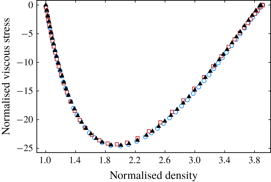
Independence validations of cell size  $\unicode[STIX]{x0394}x$, time step
 $\unicode[STIX]{x0394}t$, times of sampling
 $N_{s}$ and particle number
 $N_{p}$ for the simulation of normal shock wave in argon with
 $M_{s}=10$.
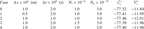
The second part of our numerical simulations is the RMI problem with specific initial conditions. Firstly, the necessity of using the DSMC method in our simulations is claimed with the local gradient-length Knudsen number  $Kn_{GL}$ in our simulations. Boyd (Reference Boyd2003) mentioned that the local gradient-length Knudsen number
 $Kn_{GL}$, which is defined as (A 1), is a critical parameter for continuum breakdown:
 $$\begin{eqnarray}Kn_{GL}=\frac{\bar{\unicode[STIX]{x1D706}}}{Q}|\unicode[STIX]{x1D735}Q|,\end{eqnarray}$$
where  $Q$ represents the flow quantities
 $(p,\unicode[STIX]{x1D70C},T,\boldsymbol{V})$ and
 $\bar{\unicode[STIX]{x1D706}}$ is the mean value of local mean free path of the gas mixture. For a specific gas, the local mean free path is calculated as
 $$\begin{eqnarray}\unicode[STIX]{x1D706}=\frac{1}{\sqrt{2}\unicode[STIX]{x03C0}{d_{ref}}^{2}n(T_{ref}/T)^{\unicode[STIX]{x1D70E}-0.5}},\end{eqnarray}$$
where  $n$ is the local number density,
 $d_{ref}$ represents the diameter of the particles at the reference temperature
 $T_{ref}=273.15~\text{K}$,
 $\unicode[STIX]{x1D70E}$ is the exponent parameter of the power-law relation for viscosity. For the mixture of gases, the mean value of the local mean free path is estimated as follows (see Bird Reference Bird1994):
 $$\begin{eqnarray}\bar{\unicode[STIX]{x1D706}}=\mathop{\sum }_{is=1}^{ns}\frac{n_{is}}{n}\unicode[STIX]{x1D706}_{is},\end{eqnarray}$$
where  $ns$ is the number of gas species, and
 $n_{is}$,
 $\unicode[STIX]{x1D706}_{is}$ are the local number density and mean free path for a specific gas species, respectively.
For instance, the local gradient-length Knudsen number  $Kn_{GL}$ based on pressure for case 0 at
 $t^{\ast }=0.8$ on the upper (
 $y=0.12$) and lower boundaries (
 $y=0$) is calculated from the simulated results, as shown in figure 14. The cutoff value of
 $Kn_{GL}$ for continuum breakdown proposed by Wang & Boyd (Reference Wang and Boyd2003) is 0.05 (red dashed line in figure 14);
 $Kn_{GL}$ is up to 0.6 inside the incident and transmitted shocks, which implies the breakdown of the continuum and the inapplicability of the classical Navier–Stokes solvers in our simulations.
The local gradient-length Knudsen number  $Kn_{GL}$ along the upper and lower boundaries of case 0 at
 $t^{\ast }=0.8$. Symbols: ○,
 $y=0.12~\text{m}$; ●,
 $y=0~\text{m}$.
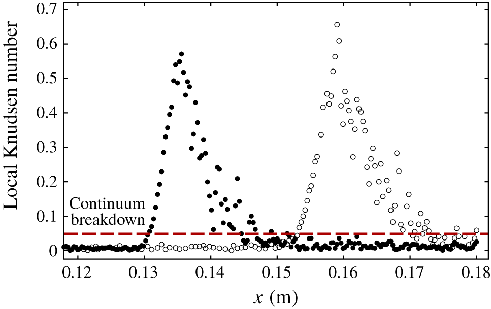
Again, the numerical accuracy mainly depends on four parameters, namely, the collisional cell size  $\unicode[STIX]{x0394}x_{c}$, the time step
 $\unicode[STIX]{x0394}t$, the times of sampling
 $N_{s}$ and the initial number of computational particles per sampling cell in the lowest density region
 $N_{p0}$.
The collision cell sizes  $\unicode[STIX]{x0394}x_{c}=6\times 10^{-5}~\text{m}$ are the same for cases 0–12 and are compared with the minimum value of local mean free path
 $\unicode[STIX]{x1D706}_{min}$. For all the cases we simulated, the flow parameters at each point of the computational domain are theoretically predicted as long as the strength of the shocks
 $M_{r},M_{t}$ are predicted by the method described in § 4.1. Then, the local mean free paths are calculated as (A 2).
For cases 0–12, the minimum value of the predicted  $\unicode[STIX]{x1D706}/\unicode[STIX]{x0394}x_{c}=3.93$ appears in the region after the transmitted shock of case 3. The mean collision times
 $\bar{\unicode[STIX]{x0394}t_{c}}$ are also predicted for cases 0–12, and the minimum value of the predicted
 $\bar{\unicode[STIX]{x0394}t_{c}}/\unicode[STIX]{x0394}t=48.3$ appears in the region after the reflected shock of case 3. Therefore, the spatial and temporal discretisation error is sufficiently small for all the simulated cases according to Alexander et al. (Reference Alexander, Garcia and Alder1998) and Garcia & Wagner (Reference Garcia and Wagner2000).
We validated the collisional cell size and the time step by simulating moving normal shock waves with the same  $\unicode[STIX]{x0394}x_{c}$ and
 $\unicode[STIX]{x0394}t$ as cases 0–12 and comparing the results with the simulated one-dimensional steady shock waves. We simulate the shock waves in argon with
 $M_{s}=8,6,4,2$ and the shock waves in helium, neon, krypton with
 $M_{s}=8$ by our two-dimensional DSMC code for unsteady flow whilst the number of cells in the
 $y$ direction is 1. The simulations of moving shocks include all the conditions of incident shock waves for cases 0–12. The number of particles
 $N_{p0}=24$ and the times of sampling
 $N_{s}=1600$ are the same as those in cases 0–12.
The computational domains are  $x\in (0,0.12)~\text{m}$ for all the simulations. The total number of the time steps is 8000, and the flow quantities are output every 200 times steps.
The computational conditions and the results of the simulations of moving shock waves are listed in table 6. The first column of table 6 indicates which of the cases from cases 0–12 have the same incident shock wave as the one simulated here. Here,  ${\mathcal{V}}_{0}^{\ast }$ is the simulated viscous source integral of the one-dimensional steady shocks and is treated as the baseline value. As claimed and verified in § 3, the normalised viscous source integral of a single shock in monatomic gas only depends on its strength
 $M_{s}$. Thus, for the shock waves with
 $M_{s}=8$ in different gases in table 6, the baseline values
 ${\mathcal{V}}_{0}^{\ast }$ are the same, which is the simulated result of the shock wave in argon;
 ${\mathcal{V}}_{s}^{\ast }$ is the simulated viscous source integral of the moving shock waves. It is an average value of the last 15 output results for every simulation.
The simulated viscous source integrals of the moving shocks with the same spatial and temporal accuracy as cases 0–12 are very close to the baseline values. This closeness validates the values of  $\unicode[STIX]{x0394}x_{c}$ and
 $\unicode[STIX]{x0394}t$ in our simulations and indirectly verifies our two-dimensional DSMC code for unsteady flow.
Again, the independence validations about  $\unicode[STIX]{x0394}x_{c}$,
 $\unicode[STIX]{x0394}t$,
 $N_{s}$ and
 $N_{p0}$ are carried out. Case 0 is taken as an example. We simulate four additional cases, with
 $\unicode[STIX]{x0394}x_{c}$,
 $\unicode[STIX]{x0394}t$,
 $N_{s}$ and
 $N_{p0}$ being changed to a high level of numerical accuracy, as listed in table 7. The simulated circulation rates
 $\dot{\unicode[STIX]{x1D6E4}}^{\ast \ast }$ and the sources
 $\dot{\unicode[STIX]{x1D6E4}}_{b}^{\ast \ast },\dot{\unicode[STIX]{x1D6E4}}_{v}^{\ast \ast }$ are compared with the original case. The simulated results of cases 1–4 are very close to the ones of case 0. This closeness validates the computational parameters of the simulations in the previous study.
Cell size  $\unicode[STIX]{x0394}x_{c}$ and time step
 $\unicode[STIX]{x0394}t$ validations by simulating moving shock waves with different initial conditions.
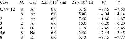
Independence validations of collision cell size  $\unicode[STIX]{x0394}x_{c}$, time step
 $\unicode[STIX]{x0394}t$, times of sampling
 $N_{s}$ and particle number
 $N_{p,0}$ for the simulation of case 0.