



1. Introduction
The marginal ice zone (MIZ) is the stretch of disordered ice floes at the interface between open water and consolidated sea ice which can be found in polar regions all year round. The dynamics of the MIZ are of interest to inform operational sea ice models for maritime operations as well as to determine momentum and heat fluxes between the ocean and atmosphere for climate modelling in polar regions. The coupling between ocean waves and sea ice is a major driver of MIZ dynamics with ocean waves fracturing ice floes, while waves are attenuated by the ice with increasing distance into the MIZ.
One side of the wave–ice coupling, the effect of sea ice on waves in the MIZ has long been the subject of field observations and modelling efforts (see Squire Reference Squire2007, Reference Squire2020). For modest sea states, field observations show that waves attenuate exponentially with distance travelled into the MIZ and that the attenuation rate increases for decreasing wave periods. It remains unclear whether scattering or dissipation is the dominant mechanism responsible for wave attenuation (Thomson Reference Thomson2022). However, field observations find that directional spread increases with distance travelled into the MIZ, suggesting multiple scattering is important (Liu et al. Reference Liu, Vachon and Peng1991; Sutherland & Gascard Reference Sutherland and Gascard2016). The rate of directional spread also increases as wave period decreases. Wadhams et al. (Reference Wadhams, Squire, Goodman, Cowan and Moore1988) observe wind sea and swell reaching isotropy after travelling
 $O(1\,\mathrm{km})$
and
 $O(10\,\mathrm{km})$
, respectively, in the MIZ.
On the other side of the wave–ice coupling, understanding the ability of waves to fracture sea ice is important because it affects the floe size distribution (FSD) and the efficacy of the MIZ to shield the pack ice beyond from wave energy. Ice floes comparable to or larger than the incident wavelength are observed to flex and fracture due to waves (Squire & Martin Reference Squire and Martin1980; Dumas-Lefebvre & Dumont Reference Dumas-Lefebvre and Dumont2023). While both determining ice deflection given an incident wave field and relating ice deflection to ice breakup present challenges, we focus on the former in this work.
Much effort has been devoted to phase-resolved numerical solutions for the ice deflection of a single ice floe given a unidirectional and monochromatic incident wave, starting with simple shapes (Meylan & Squire Reference Meylan and Squire1996; Porter Reference Porter2019) and generalized to arbitrary geometries (Meylan Reference Meylan2002; Bennetts & Williams Reference Bennetts and Williams2010; Li et al. Reference Li, Shi, Shao and Ning2024). One of the main takeaways from these studies is that geometry is important to the location and magnitude of the maximum strain when the ice floe size is comparable to the wavelength.
Modelling ice breakup and FSD evolution at the MIZ scale requires trade-offs between fidelity and computational expense. Phase-resolved methods (e.g. Montiel et al. Reference Montiel, Squire and Bennetts2016) capture the floe geometry-dependent ice deflection and model multiple scattering in a realistic FSD but are too computationally intensive for large-scale modelling. Phase-averaged models of wave–ice interactions, based on radiative transport theory, describe the evolution of wave intensity in the MIZ and offer a useful balance of fidelity and computational expense. These are implemented in large-scale spectral wave models, such as WaveWatch3, and wave-in-ice models (e.g. Williams et al. Reference Williams, Rampal and Bouillon2017), which are developed for operational forecasting and climate modelling.
Phase-averaged methods typically determine the spectrum of ice deflection from the wave elevation spectrum in the surrounding open water through conservation of energy flux (Wadhams Reference Wadhams1973; WW3DG 2016). This accounts for the change in group speed and the addition of flexural energy to the partitioning of wave energy in the ice-covered region. However, this approach does not account for reflection and transmission at the ice edge, including the role of oblique incidence. Additionally, the conservation of energy flux approach is not a function of the size or plan form of the ice sheet, only its stiffness (and the contribution of ice inertia). It is clear that an ice sheet much smaller than the wavelength behaves differently than an ice sheet much larger than the wavelength, so there must be some range of validity to ascertain.
Our main interest in this work is to derive theoretical expressions, independent of the ice plan form, relating the wave intensity in an ice floe within the MIZ to the wave intensity in the open water surrounding it. Intensity is defined as directional wave energy flux density. We consider the ice floe to be located sufficiently far within the MIZ so that the wave field in the surrounding open water is isotropic due to multiple scattering. We consider a narrow-banded wave spectrum, typical of realistic ocean conditions, as opposed to a monochromatic incident wave. We consider the spacing between ice floes to be large enough that the incident wave field consists of only propagating, not evanescent, modes. We check the range of validity of the theoretical results with direct computational results for simple ice shapes.
Our theoretical approaches are based on results from optics used to define upper bounds on solar cell performance. These efforts began in the ray optical regime for thick solar cells (Yablonovitch Reference Yablonovitch1982; Green Reference Green2002), which inspire our short-wavelength asymptotic (SWA) result. More recent works seek to outperform the ray optical result by considering solar cells with subwavelength thickness, requiring new theoretical approaches (Yu et al. Reference Yu, Raman and Fan2010; Taflove et al. Reference Taflove, Oskooi and Johnson2013). The Green function result we derive is inspired by this line of work, specifically Benzaouia et al. (Reference Benzaouia, Tokić, Miller, Yue and Johnson2019).
The problem statement and boundary value problem are specified in § 2 where we assume linear wave theory, an incoherent, isotropic, narrow-banded incident wave spectrum and linear elastic ice behaviour. In § 3, we derive a SWA result for
 $k^I\ell \gg 1$
, where
 $k^I=2\pi /\lambda ^I$
is the wavenumber in ice and
 $\ell$
is the length scale of the ice sheet. The SWA result shows that the intensity in ice is reduced from the intensity in the surrounding open water by the ratio of wavenumbers in ice and open water. This result provides a clear insight that the reduction in intensity is related to the total reflection for a portion of the incident wave angles from open water. The SWA, however, assumes
 $\ell \gg \lambda ^I$
from the outset which does not provide insight into its range of validity in terms of
 $k^I\ell$
. We derive a more general result in § 4 where we apply reciprocity to the boundary value problem to relate the wave intensity reduction in ice to a Green function describing time-harmonic point forcing on the ice sheet. By locally approximating the Green function for a general ice sheet plan form with the Green function for an infinite-extent ice sheet, we obtain a general result which recovers SWA for
 $k^I\ell \gg 1$
, but is also applicable for a larger parameter space in terms of
 $\ell _D/\ell$
, where
 $\ell _D$
is the flexural-gravity length scale, regardless of
 $k^I\ell$
.
We elucidate the theoretical results by considering a circular ice sheet as an example in § 5 for which we can solve for the wave response to an isotropic wave field numerically. We switch from intensity to squared amplitude when comparing theoretical and computational results because the latter is defined unambiguously everywhere in the ice sheet and is related to important physical quantities. In § 5.1, we show that the intensity matches the theoretical results in the bulk of the ice sheet. In § 5.2, we establish that the increase in squared amplitude near the ice edge is independent of ice plan form for
 $k^I\ell \gg 1$
. With this insight, we develop an edge correction to the theoretical results which is a good approximation of the squared amplitude in the entire ice sheet. We discuss the range of validity of the theoretical results with respect to
 $k^I\ell$
in § 5.3, and we elucidate the role of ice stiffness in terms of
 $\ell _D$
(§ 5.4). In § 6, we provide further evidence of the plan form independence of the theoretical results by considering rectangular ice sheets. In § 7, we consider the performance of the theoretical results when the incident wave field has not yet reached isotropy. We briefly summarize in § 8.
2. Problem definition
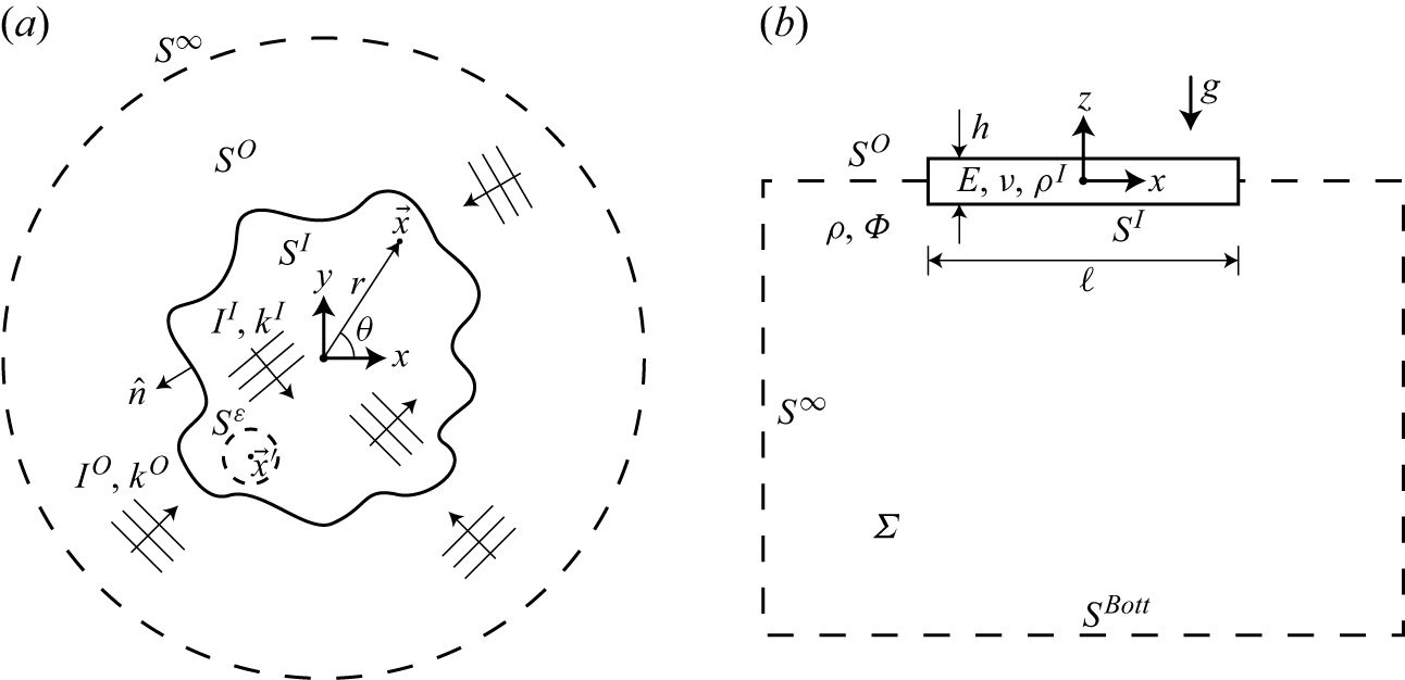
We consider a single floating ice sheet of arbitrary plan form immersed in an isotropic incident wave field (see figure 1). We model the ice sheet as a thin, uniform elastic plate of shallow draft with ice density
 $\rho ^I$
, elastic modulus
 $E$
, thickness
 $h$
and Poisson ratio
 $\nu$
with flexural rigidity
 $D = Eh^3/(12(1-\nu ^2))$
. For simplicity, we consider a fluid of infinite depth, and assume potential flow and linear wave theory throughout. We further assume that waves propagate through the ice sheet without dissipation although it would be straightforward to include dissipation in the results we present. We define a coordinate system
 $\{\boldsymbol{x}=(x,y), z\}$
with the origin located at the centre of the ice sheet with
 $z=0$
corresponding to the mean free surface. Here
 $z$
is positive upward and gravitational acceleration
 $g$
acts in the negative
 $z$
direction. We let
 $S^I$
be defined as the ice-covered region with
 $\partial S^I$
as its boundary. For ice sheet plan forms that can be described by a single length scale, we define a characteristic length scale
 $\ell =\sqrt {\mathcal{A}}$
where
 $\mathcal{A}$
is the plan form area of the ice sheet.
Problem definition sketch: (a) top and (b) side view.

We denote wave intensity
 $I$
, directional wave amplitude
 $A$
and wavenumber magnitude
 $k$
with superscripts
 $O$
and
 $I$
referring to open water and ice, respectively. We consider the wave spectra in open water and in ice to have narrow bandwidth
 $\Delta k/k_c$
where
 $k_c$
denotes the centre wavenumber, and we use a ‘top hat’ incident wave spectrum for simplicity.
The flow can be described by a time-harmonic velocity potential
 $\varPhi (\boldsymbol{x},z,t) = \mathrm{Re}\{\varphi (\boldsymbol{x},z)\exp (-\mathrm{i}\omega t)\}$
which satisfies the following governing equation and boundary conditions:
 \begin{equation} {\nabla} ^2\varphi = 0, \quad \forall \;\boldsymbol{x},\; z\lt 0 , \end{equation}
 \begin{equation} \big (\ell _D^4 {\nabla} _{\boldsymbol{x}}^4 + 1 - \gamma k^O \big )\varphi _z - k^O \varphi = 0, \quad \boldsymbol{x}\in S^I,\; z=0 , \end{equation}
 \begin{equation} \varphi _z - k^O \varphi = 0, \quad \boldsymbol{x}\in S^O,\; z=0 , \end{equation}
 \begin{equation} |\boldsymbol{\nabla }\varphi |\to 0, \quad \forall \;\boldsymbol{x}, \; z\to -\infty , \end{equation}
where
 $\ell _D = (D/(\rho g))^{1/4}$
is the flexural-gravity length scale,
 $\gamma = (\rho ^I h)/\rho$
,
 $k^O = \omega ^2/g$
and
 $\rho$
is water density. Here
 ${\nabla} _{\boldsymbol{x}}^4$
denotes the biharmonic operator in the horizontal plane. We impose free–free edge conditions and appropriate corner constraints on
 $\partial S^I$
as described by Bennetts & Williams (Reference Bennetts and Williams2010) for ice floes of arbitrary shape. The accompanying time-harmonic free surface elevation
 $\xi (\boldsymbol{x},t) = \mathrm{Re}\{\eta (\boldsymbol{x})\exp (-\mathrm{i}\omega t)\}$
is related to the velocity potential by
 $\eta = (\mathrm{i}/\omega ) \varphi _z|_{z=0}$
.
3. Asymptotic result for wave intensity in an ice sheet for a wavelength that is short compared with the floe dimension
We first derive a SWA result for
 $k^I\ell \gg 1$
, in the spirit of Yablonovitch (Reference Yablonovitch1982), where we assume uniform and isotropic wave intensity in both the ice sheet and the surrounding open water. We begin by invoking conservation of energy flux
 $\boldsymbol{\mathcal{F}}$
across the ice edge
 $\partial S^I$
with outward-facing normal
 $\hat {n}$
:
 \begin{equation} \int _{\partial S^I} \boldsymbol{\mathcal{F}}(\boldsymbol{x})\boldsymbol{\cdot }\hat {n} {\rm d}s = 0. \end{equation}
We now decompose the vector flux density
 $\boldsymbol{\mathcal{F}}(\boldsymbol{x})$
into emitted
 $\mathcal{F}^+(\boldsymbol{x},\hat {n})$
and incoming
 $\mathcal{F}^-(\boldsymbol{x},\hat {n})$
scalar flux densities where
 $\boldsymbol{\mathcal{F}}(\boldsymbol{x})\boldsymbol{\cdot }\hat {n} = \mathcal{F}^+(\boldsymbol{x},\hat {n}) - \mathcal{F}^-(\boldsymbol{x},\hat {n})$
. The scalar flux densities are defined in terms of intensity as follows:
 \begin{gather} \mathcal{F}^\pm (\boldsymbol{x},\hat {n}) = \int _{\hat {e}_\sigma \boldsymbol{\cdot }\hat {n}\gtrless 0}I(\boldsymbol{x},\hat {e}_\sigma )\hat {e}_\sigma \boldsymbol{\cdot }\hat {n}{\rm d}\sigma , \end{gather}
where
 $\hat {e}_\sigma$
is a unit vector in the
 $x$
–
 $y$
plane. In open water and in the ice sheet, regions exist sufficiently close to the ice edge where both propagating and spatially decaying modes contribute to the wave intensity, which we refer to as edge-affected regions and denote as
 $S^O_e$
and
 $S^I_e$
, respectively. Outside of these regions where only the propagating mode contributes, we consider the frequency-averaged (denoted by
 $\langle \boldsymbol{\cdot }\rangle _\omega$
) wave intensity to be isotropic,
 $\langle I^{O,I}\rangle _\omega \neq \langle I^{O,I}(\hat {e}_\sigma )\rangle _\omega$
, and uniform,
 $\langle I^{O,I}\rangle _\omega \neq \langle I^{O,I}(\boldsymbol{x})\rangle _\omega$
, for
 $\boldsymbol{x}\in S^{O,I}/S^{O,I}_e$
, in both the open water and ice-covered regions. Note that frequency averaging is a natural consequence of a realistic narrow-banded wave spectrum. Without frequency-averaging, i.e. with a monochromatic incident wave,
 $I^I$
exhibits a wavelength-scale interference pattern and cannot be assumed uniform and isotropic.
Under these assumptions, the wave intensity in open water and in the ice sheet away from the ice edge, for a single frequency are, respectively,
 \begin{equation} I^O = \frac {1}{2}\rho \frac {\omega ^2}{k^O} C_g^O|A^O|^2, \end{equation}
 \begin{equation} I^I = \frac {1}{2}\rho \frac {\omega ^2}{k^I}(1 + \gamma k^I)C_g^I|A^I|^2, \end{equation}
where
 $C_g^O=\omega /(2k^O)$
and
 $C_g^I = (\omega /(2k^I) + 2D(k^I)^4/(\rho \omega ))/(1+\gamma k^I)$
are the group speed in open water and ice, respectively. These definitions of intensity resemble those of wave energy flux for a plane progressive wave but differ as
 $A$
refers to directional amplitude (amplitude per radian) in the current context. For reference, the dispersion relations in the open water and ice-covered regions are
 $\omega ^2 = gk^O$
and
 $\omega ^2 = (gk^I + D(k^I)^5/\rho )/(1+\gamma k^I)$
, respectively.
With these assumptions, the flux density does not vary along the ice edge, so we proceed by considering the flux balance (3.1) at a single element
 ${\rm d}s$
. We express the integrals in terms of
 $\hat {e}_\sigma \boldsymbol{\cdot }\hat {n} =\cos \theta$
and
 $\hat {e}_\sigma \boldsymbol{\cdot }-\hat {n} =\cos \psi$
as follows:
 \begin{equation} \bigl \lt \left (\mathcal{F}^+ - \mathcal{F}^-\right ) {\rm d}s \bigr \gt _\omega = \left \lt \left (\int _{-\pi /2}^{\pi /2}I(\theta )\cos \theta {\rm d}\theta - \int _{-\pi /2}^{\pi /2}I(\psi )\cos \psi {\rm d}\psi \right ) {\rm d}s \right \gt _\omega = 0. \end{equation}
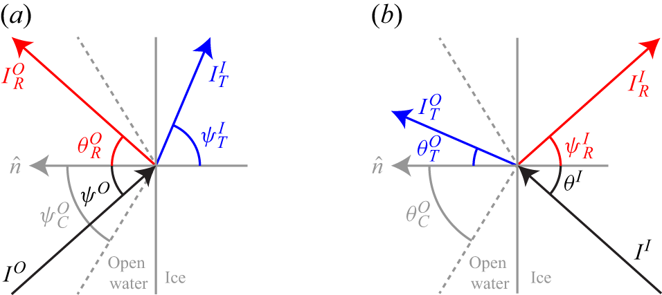
Intensities at the ice edge for waves propagating from (a) open water into ice and (b) ice into open water.

We apply (3.4) to the ice-covered side of the ice edge. Our interest is when the ice sheet is large compared with the wavelength (
 $k^I\ell \gg 1$
) where a small element
 ${\rm d}s$
of the ice edge can be treated as a planar interface between open water and the ice sheet. For
 $k^I\ell \gg 1$
,
 $S_e^{O,I}\ll S^I$
so we consider only the propagating mode when performing the flux balance. For each intensity
 $I$
and angle
 $\theta$
or
 $\psi$
, the subscripts
 $R$
and
 $T$
denote reflected and transmitted components, respectively, with no subscript indicating an incident component. On the ice-covered side, we must account for the flux from the incident intensity in ice
 $I^I$
, the reflected intensity in ice
 $I^I_R$
and the transmitted intensity from open water into the ice
 $I^I_T$
(see figure 2):
 \begin{equation} \Biggl \lt I^I\int _{-\pi /2}^{\pi /2}\cos \theta ^I {\rm d}\theta ^I-\int _{-\pi /2}^{\pi /2}I^I_R\cos \psi ^I_R {\rm d}\psi ^I_R - \int _{-\pi /2}^{\pi /2}I^I_T\cos \psi ^I_T {\rm d}\psi ^I_T \Biggr \gt _\omega = 0. \end{equation}
We now relate (
 $I^I_R$
,
 $\psi ^I_R$
) and (
 $I^I_T$
,
 $\psi ^I_T$
) to (
 $I^I$
,
 $\theta ^I$
) and (
 $I^O$
,
 $\psi ^O$
), respectively. Here
 $\psi _R^I=\theta ^I$
, trivially, and
 $ I^I_R = |\tilde {R}(\theta ^I)|^2I^I$
where
 $\tilde {R}$
is the wave amplitude reflection coefficient for a wave propagating from ice into open water. To find
 $I^I_T$
, we equate the incident flux from open water onto a small element
 $ds$
with the sum of the reflected and transmitted fluxes (in the manner of Ishimaru Reference Ishimaru1997) (see figure 2
a):
 \begin{equation} \Biggl \lt I^O\int _{-\pi /2}^{\pi /2} \cos \psi ^O {\rm d}\psi ^O \Biggr \gt _\omega = \Biggl \lt \int _{-\pi /2}^{\pi /2}I^O_R \cos \theta ^O_R {\rm d}\theta ^O_R + \int _{-\pi /2}^{\pi /2}I^I_T \cos \psi ^I_T {\rm d}\psi ^I_T \Biggr \gt _\omega . \end{equation}
We simplify (3.6) by recognizing that
 $\theta ^O_R = \psi ^O$
and
 $I^O_R = |R(\psi ^O)|^2I^O$
where
 $R$
is the wave amplitude reflection coefficient for a wave propagating from open water into ice. The limits of the integral with respect to
 $\psi ^O$
change from
 $ [-\pi /2,\pi /2 ]$
to
 $ [-\psi ^O_c,\psi ^O_c ]$
where the critical angle for waves propagating from open water into ice is
 $\psi ^O_c=\theta _c^O= \arcsin (k^I/k^O)$
. This is because
 $|R(\psi ^O)|^2 = 1$
for
 $\psi ^O_c\leqslant |\psi ^O|\leqslant \pi /2$
. Equation (3.6) then becomes
 \begin{equation} \Biggl \lt I^O\int _{-\psi ^O_c}^{\psi ^O_c}(1-|R(\psi ^O)|^2) \cos \psi ^O {\rm d}\psi ^O \Biggr \gt _\omega = \Biggl \lt \int _{-\pi /2}^{\pi /2}I^I_T \cos \psi ^I_T {\rm d}\psi ^I_T \Biggr \gt _\omega . \end{equation}
We perform a change of variables using Snell’s law:
 $k^O \sin \psi ^O = k^I \sin \psi ^I_T$
(with differential form
 $k^O \cos \psi ^O {\rm d}\psi ^O= k^I \cos \psi ^I_T {\rm d}\psi ^I_T$
). Equation (3.7) then simplifies to
 \begin{equation} \Biggl \lt I^O\int _{-\pi /2}^{\pi /2}\left (1-|R(\psi ^O)|^2\right ) \frac {k^I}{k^O}\cos \psi ^I_T {\rm d}\psi ^I_T \Biggr \gt _\omega = \Biggl \lt \int _{-\pi /2}^{\pi /2}I^I_T \cos \psi ^I_T {\rm d}\psi ^I_T \Biggr \gt _\omega . \end{equation}
We combine (3.5) and (3.8) to give
 \begin{align} \Biggl \lt I^I\int _{-\pi /2}^{\pi /2}\left (1-|\tilde {R}(\theta ^I)|^2\right )\cos \theta ^I {\rm d}\theta ^I \Biggr \gt _\omega = \Biggl \lt I^O\frac {k^I}{k^O}\int _{-\pi /2}^{\pi /2}\left (1-|R(\psi ^O)|^2\right ) \cos \psi ^I_T {\rm d}\psi ^I_T \Biggr \gt _\omega . \end{align}
It can be shown using a time reversal argument (similar to Meylan & Squire (Reference Meylan and Squire1993)) that
 $\left |R (\psi ^O )\right | = |\tilde {R}(\theta ^I)|$
. We arrive at the main result under the assumption of
 $k^I_c\ell \gg 1$
,
 \begin{equation} \langle I^I \rangle _\omega = \biggl \lt \frac {k^I}{k^O}I^O \biggr \gt _\omega \equiv \langle I^I_b \rangle _\omega , \end{equation}
where, for later reference, we denote the theoretical result as
 $\langle I^I_b \rangle _\omega$
. Since
 $k^I$
is typically less than
 $k^O$
, (3.10) shows that the wave intensity is generally reduced in the ice. This is due to total reflection for waves propagating from open water into the ice sheet with incident angle greater than the critical angle predicted by Snell’s law. To reiterate, (3.10) is derived assuming a uniform, isotropic and narrow-banded wave field within the ice sheet and in the surrounding open water in the limit of
 $k^I\ell \gg 1$
. The result does not depend on the specific ice sheet geometry. The SWA is useful for its simplicity and for the physical intuition it provides.
This general approach is inspired by the known theoretical short wavelength limit on the internal light intensity in a solar cell,
 $I^{Int}$
, immersed in isotropic external incident light of intensity
 $I^{Ext}$
:
 $I^{Int} = 2n^2I^{Ext}$
, where
 $n$
is the index of refraction (Yablonovitch Reference Yablonovitch1982). In that context, for a typical material such as silicon with
 $n\approx 3.5$
, the theoretical limit predicts an intensity enhancement of
 $I^{Int}/I^{Ext} \approx 25$
due to light trapping resulting from total internal reflection within the solar cell.
The wave–ice interaction differs from the solar cell in two major ways. First, for the same frequency, the wavelength is typically greater in ice than in open water, so a critical angle exists for waves propagating from open water into ice. On the other hand, the wavelength of light is less in silicon than in air, such that a critical angle exists for waves propagating from silicon into air. Consequently, total reflection reduces the intensity in ice compared with the surrounding open water while increasing the intensity in silicon compared with the surrounding air. Second, a solar cell is three-dimensional while an ice sheet subject to surface waves is effectively two-dimensional. This reduction in dimension explains the difference between
 $I^{Int} = 2n^2I^{Ext}$
in three dimensions for a solar cell and
 $I^I = \tilde {n}I^O$
in two dimensions for waves in ice where
 $\tilde {n} = k^I/k^O$
.
4. General result for wave intensity in ice using the Green function
It is useful to derive a more general result without making the SWA assumption of
 $k^I\ell \gg 1$
from the outset. Here we apply reciprocity to the boundary value problem (2.1) directly to derive a general result applicable for all
 $k^I\ell$
. This approach is similar to what Benzaouia et al. (Reference Benzaouia, Tokić, Miller, Yue and Johnson2019) apply to Maxwell’s equations to relate the intensity enhancement in a solar cell to the local density of states. We begin by defining a Green function which describes the response of the ice and the surrounding open water to a time-harmonic point forcing on the ice surface. We utilize this Green function to obtain two intermediate results using Green’s second identity. First, we derive a relationship between the power input at the location of the point forcing and the total radiated energy flux in the surrounding open water. Second, we derive a reciprocity relation connecting the ice deflection due to a plane wave from a single incident direction to the far-field of the Green function in the direction opposite that of the incident wave. We combine these two results to relate the ice deflection due to an isotropic incident wave field to the Green function evaluated at the forcing location. We show that (3.10) is recovered by approximating the Green function for an ice sheet of general plan form evaluated at the forcing location with the closed-form Green function for an ice sheet of infinite extent.
We define the Green function
 $G(\boldsymbol{x}, z; \boldsymbol{x}')$
which satisfies (2.1) and the edge/corner conditions with the exception that the dynamic boundary condition (2.1b
) is modified to include time-harmonic point forcing,
 \begin{equation} (\ell _D^4 {\nabla} _{\boldsymbol{x}}^4 + 1 - \gamma k^O)G_z - k^O G = \mathrm{i} \omega \frac {F}{\rho g}\delta ^2(\boldsymbol{x} - \boldsymbol{x}'), \quad (\boldsymbol{x},\boldsymbol{x}')\in S^I,\; z=0 , \end{equation}
where
 $F$
is the complex amplitude of the force applied at
 $\boldsymbol{x}=\boldsymbol{x}'$
. The far-field approximation of the Green function in the open water surrounding the ice sheet is expressed as
 \begin{equation} G \approx -\mathrm{i} \frac {\omega }{k^O}\exp (k^O z)a^\infty (\theta ;\boldsymbol{x}')\sqrt {\frac {2}{\pi k^O r}}\exp (\mathrm{i} k^Or - \mathrm{i}\pi /4), \quad k^O r\gg 1, \end{equation}
where
 $r=\lVert \boldsymbol{x}-\boldsymbol{x}'\rVert$
,
 $\theta$
is the angle between
 $\boldsymbol{x}-\boldsymbol{x}'$
and the
 $x$
-axis and
 $a^\infty$
is the far-field (complex) amplitude in direction
 $\theta$
due to point forcing at
 $\boldsymbol{x}'$
.
We define the control volume used when applying Green’s second identity in the following subsections. Referring to figure 1, we consider the fluid region
 $\varSigma$
bounded above by the mean position of the ice sheet
 $S^I$
and the surrounding open water
 $S^O$
at
 $z=0$
, separated by the ice edge
 $\partial S^I$
. Within
 $S^I$
, we define
 $S^\varepsilon$
, a circular region with radius
 $\varepsilon$
encompassing the source point of the Green function. Here
 $\varSigma$
is bounded from below by a horizontal control surface
 $S^{Bott}$
at
 $z\to -\infty$
. The radial extent of
 $\varSigma$
is bounded by a cylindrical control surface in the far field
 $S^\infty$
centred at the origin with radius
 $r^\infty$
such that
 $k^Or^\infty \gg 1$
.
4.1. Radiation damping due to time-harmonic point forcing on ice
We apply Green’s second identity to the Green function and its complex conjugate, denoted with an asterisk:
 \begin{equation} 2\mathrm{i} \, \mathrm{Im}\biggl \{\int _{S^I/S^\varepsilon }G G_z^*{\rm d}S + \int _{S^\infty }G G_r^*{\rm d}S\biggr \} = 0 . \end{equation}
To evaluate the first term of (4.3), we use
 $G = ( {1}/{k^O})(\ell _D^4 {\nabla} _{\boldsymbol{x}}^4 + 1 - \gamma k^O)G_z$
, valid for
 $\boldsymbol{x}\in S^I$
except at
 $\boldsymbol{x}=\boldsymbol{x}'$
, to find
 \begin{equation} 2\mathrm{i} \, \mathrm{Im}\biggl \{\int _{S^I/S^\varepsilon }G G_z^*{\rm d}S\biggr \} = 2\mathrm{i} \, \mathrm{Im}\biggl \{\int _{S^I}\frac {\ell _D^4}{k^O} ({\nabla} _{\boldsymbol{x}}^4G) G_z^*{\rm d}S - \int _{S^\varepsilon }\frac {\ell _D^4}{k^O} ({\nabla} _{\boldsymbol{x}}^4G) G_z^*{\rm d}S \biggr \} . \end{equation}
It can be shown using Green’s first identity and the free–free edge conditions that the first term on the right-hand side of (4.4) evaluates to zero because the edges are not a source or sink of power. We evaluate the second term by multiplying (4.1) by
 $G_z^*$
, integrating over
 $S^\varepsilon$
and taking the limit as
 $\varepsilon \to 0^+$
(where only the biharmonic term and delta function contribute), resulting in a final expression as
 \begin{equation} 2\mathrm{i} \, \mathrm{Im}\biggl \{\int _{S^I/S^\varepsilon }G G_z^*{\rm d}S\biggr \} = 2\mathrm{i} \frac {\omega }{\rho g} \mathrm{Re} \big\{ F G_z^*(\boldsymbol{x}',0;\boldsymbol{x}') \big\} . \end{equation}
It is straightforward to evaluate the second term of (4.3) using the far-field approximation (4.2). The complete expression resulting from (4.3) is
 \begin{equation} -\mathrm{Re}\{F G_z^*(\boldsymbol{x}',0;\boldsymbol{x}')\} = \rho g C_g^O \frac {2}{\pi k^O}\int _0^{2\pi }|a^\infty (\theta ;\boldsymbol{x}')|^2{\rm d}\theta . \end{equation}
Equation (4.6) resembles expressions describing the radiation damping of a floating rigid body in simple harmonic motion (see (8.6.13), Mei et al. (Reference Mei, Stiassnie and Yue2005)); however, the Green function evaluated at its source point takes the place of radiation potentials for discrete modes.
4.2. Reciprocity relation for a single incident direction
We now derive a reciprocity relation between the Green function and a velocity potential
 $\phi (\boldsymbol{r},z;\theta _0)$
satisfying (2.1) and the edge/corner conditions which represents a plane progressive incident wave propagating in direction
 $\theta _0$
interacting with the ice sheet. This potential has a far-field approximation for
 $k^Or\gg 1$
,
 \begin{align} \phi \approx -\mathrm{i}\frac {\omega }{k^O}A^O\exp (k^Oz)\left ( \exp (\mathrm{i} k^Or \cos (\theta -\theta _0)) + \sqrt {\frac {2}{\pi k^O r}}\mathcal{A}(\theta ;\theta _0)\exp (\mathrm{i} k^O r - \mathrm{i} \pi /4)\right )\!, \end{align}
where
 $\mathcal{A}(\theta ;\theta _0)$
denotes the scattered wave amplitude in direction
 $\theta$
due to an incident wave from direction
 $\theta _0$
, normalised by
 $A^O$
, the amplitude of the incident wave in open water.
We once again apply Green’s second identity:
 \begin{equation} \int _{S^I/S^\varepsilon }(\phi G_z - G \phi _z){\rm d}S + \int _{S^\infty }(\phi G_r - G \phi _r){\rm d}S = 0. \end{equation}
We follow a similar procedure to § 4.1 to evaluate the first term of (4.8). For the second, far-field term involving (4.2) and (4.7), we recognize that the scattered wave field does not contribute and employ the method of stationary phase to evaluate in a straightforward manner. The reciprocity relation between the Green function and a unidirectional incident wave is
 \begin{equation} -\mathrm{i} \omega F \eta (\boldsymbol{x}';\theta _0) = \frac {4}{k^O}\rho g C_g^OA^Oa^\infty (\theta _0+ \pi ; \boldsymbol{x}'), \end{equation}
where we have used the kinematic boundary condition to relate
 $\phi$
and
 $\eta$
. Equation (4.9) resembles the Haskind–Hanoaka theorem (see (8.6.41), Mei et al. (Reference Mei, Stiassnie and Yue2005)), but instead relates the free surface elevation at
 $\boldsymbol{x} = \boldsymbol{x}'$
in the ice-covered region due to an incident plane wave to the far-field amplitude of the radiated wave generated by a time-harmonic point forcing applied at
 $\boldsymbol{x} = \boldsymbol{x}'$
.
4.3. Reciprocity theorem for isotropic incidence
We derive an expression connecting
 $G(\boldsymbol{x}',0;\boldsymbol{x}')$
to the free surface elevation at
 $\boldsymbol{x}'$
due to an incoherent, isotropic incident wave field by relating (4.6) and (4.9) in the far field. We multiply (4.9) by its complex conjugate and angle average with respect to
 $\theta _0$
by integrating from
 $0$
to
 $2\pi$
. The angle-averaged, far-field squared amplitude now appears in both expressions that we substitute to yield
 \begin{equation} |A^I(\boldsymbol{x}')|^2 = -\frac {2\rho g|A^O|^2}{(k^O)^2 \omega |F|^2}\mathrm{Re} \big\{F G_z^*(\boldsymbol{x}',0;\boldsymbol{x}') \big\}, \end{equation}
where
 $|A^I(\boldsymbol{x}')|^2 = ({1}/{2\pi })\int _0^{2\pi }|\eta (\boldsymbol{x}'; \theta _0)|^2 {\rm d}\theta _0$
. Note that (4.10) is applicable without frequency averaging and makes no assumption regarding
 $k^I\ell$
.
In general, the Green function cannot be expressed in closed form and is a function of the ice sheet plan form via the ice edge boundary conditions. However, the influence of the ice edge boundary conditions is limited to a region near the ice edge
 $S^I_e$
. Based on this intuition, we assume
 \begin{equation} \langle \mathrm{Re}\{F G_z^*(\boldsymbol{x}',0;\boldsymbol{x}')\}\rangle _\omega \approx \langle \mathrm{Re}\{F (G_z^\infty (\boldsymbol{x}',0;\boldsymbol{x}'))^*\} \rangle _\omega , \quad \boldsymbol{x}'\in S^I/S^I_e, \end{equation}
where
 $G^\infty$
is the Green function for an ice sheet of infinite spatial extent.
Fox & Chung (Reference Fox and Chung1999) derive a closed-form expression for
 $G^\infty$
in the deep-water limit which contains propagating and spatially decaying wave components. We are interested in only the real part per (4.10) to which only the propagating component contributes:
 \begin{equation} \mathrm{Re}\{F (G_z^\infty (\boldsymbol{x}',0;\boldsymbol{x}'))^*\} = -\frac {|F|^2\omega }{2\rho g}\frac {(k^I)^2}{5(\ell _Dk^I)^4 + 1-\gamma k^O}. \end{equation}
We frequency average the general reciprocity theorem for isotropic incidence (4.10) and (4.12) and substitute, which yields
 \begin{equation} \bigl \lt |A^I(\boldsymbol{x}')|^2 \bigr \gt _\omega = \biggl \lt \left (\frac {k^I}{k^O}\right )^2 \frac {|A^O|^2}{5 (\ell _Dk^I)^4 + 1 - \gamma k^O} \biggr \gt _\omega \equiv \bigl \lt |A^I_b|^2 \bigr \gt _\omega , \quad \boldsymbol{x}'\in S^I/S^I_e. \end{equation}
We can recast (4.13) using the definitions of intensity (3.3) to yield
 \begin{equation} \langle I^I(\boldsymbol{x}')\rangle _\omega = \biggl \lt \frac {k^I}{k^O}I^O \biggr \gt _\omega \equiv \langle I^I_b\rangle _\omega \;, \quad \boldsymbol{x}'\in S^I/S^I_e. \end{equation}
We use
 $|A^I_b|^2$
and
 $I^I_b$
to denote the theoretical predictions valid in the bulk of the ice sheet. We note that the Green function result here contains the SWA result of § 3 because (4.11) becomes valid everywhere in the ice sheet (except at the ice edge) in the limit as
 $k^I_c\ell \to \infty$
. As a consequence, (4.14) is equivalent to (3.10) in this limit.
We ascertain the range of validity of the approximation (4.11) in § 5.1 by comparing the closed-form expression for
 $\langle \mathrm{Re}\{F (G_z^\infty (\boldsymbol{x}',0;\boldsymbol{x}'))^*\} \rangle _\omega$
with the numerical solution for
 $\langle \mathrm{Re}\{F G_z^*(\boldsymbol{x}',0;\boldsymbol{x}')\}\rangle _\omega$
for a circular ice sheet. We find that the approximation is valid in the bulk of the ice sheet, except near the ice edge which is influenced by the free–free edge conditions. We explain in § 5.4 that this edge-affected region is small compared with the bulk of the ice sheet not only for
 $k^I_c\ell \gg 1$
but also when
 $\ell /\ell _D\gg 1$
, regardless of
 $k^I_c\ell$
. Here
 $\ell /\ell _D\gg 1$
signifies that the size of the ice sheet is large compared with the flexural-gravity length scale
 $\ell _D$
which can be much less than
 $\lambda ^I_c$
for low ice stiffness. The Green function result, therefore, has a broader range of applicability than the SWA result.
5. Elucidation of the theoretical results using a circular ice sheet
We elucidate the range of validity of the theoretical results in §§ 3–4 by considering a circular ice sheet of radius
 $R(=\ell /\sqrt {\pi })$
as an example. We reiterate that the theoretical results do not depend on ice plan form which we support by considering other shapes in § 6. In § 5.1, we compare the theoretical results with the direct computational solution of the boundary value problem (2.1) for cases where
 $k^{I} R \gg 1$
. We consider isotropic incident wave forcing as well as point forcing to determine the Green function of § 4. We show that the wave intensity away from the ice edges is uniform and agrees with (3.10) and (4.14), which are equivalent and both applicable when
 $k^{I}R\gg 1$
. To approximate the increasing squared amplitude near the ice edge, we devise an edge correction to the theoretical result using the semi-infinite ice sheet solution in § 5.2. We determine the range of validity of the theoretical results by examining the spatial mean of squared amplitude
 $\langle |A^I|^2\rangle _{\boldsymbol{x}}$
as a function of
 $k^{I}R$
in § 5.3. We address the role of ice stiffness in the range of validity of the theoretical result in § 5.4. We show that the edge-affected region is small compared with the bulk when the ice sheet radius
 $R$
is large compared with the flexural-gravity length scale
 $\ell _D$
(
 $R/\ell _D\gg 1$
) even when
 $k^{I}R=O(1)$
.
We briefly summarize the computational approach used to solve the boundary value problem (2.1) for a circular ice sheet either with an isotropic incident wave field or with point forcing (4.1) to determine the Green function. For an isotropic incident wave field, we use the method described in Peter et al. (Reference Peter, Meylan and Chung2004) to solve for the phase-resolved ice deflection
 $\eta ^I$
due to a unidirectional and monochromatic plane incident wave of unit amplitude. We repeat the numerical solution for a range of incident wave directions
 $\theta \in [0,2\pi ]$
and wavenumbers (in ice)
 $k^I\in [k^I_c-\Delta k^I, k^I_c+\Delta k^I]$
to obtain the angle- and frequency-averaged squared amplitude in the ice-covered region:
 \begin{equation} \langle |A^I(\boldsymbol{x})|^2\rangle _\omega = \frac {1}{2\Delta k^I}\int _{k^I_c-\Delta k^I}^{k^I_c+\Delta k^I}\left (\frac {1}{2\pi }\int _0^{2\pi }|\eta ^I(\boldsymbol{x}; \theta )|^2 {\rm d}\theta \right ) {\rm d}k^I. \end{equation}
Going forward, we omit
 $\langle \boldsymbol{\cdot }\rangle _\omega$
, with frequency averaging over the (narrow) incident wave band implied. After performing convergence testing with respect to
 $\langle |A^I|^2\rangle _{\boldsymbol{x}}$
, we use 40 azimuthal modes, 28 roots of the dispersion relation,
 $N_\theta = 32$
discrete incident wave directions,
 $N_\omega =17$
discrete frequencies and water depth
 $H$
such that
 $k^I_cH = 13.4$
to approximate the deep water limit. We expect the numerical error to be less than 1 % for this selection of parameters.
We determine the Green function by making a simple modification to the eigenfunction matching method of Zheng et al. (Reference Zheng, Michele, Liang, Meylan and Greaves2022) to study wave power extraction by an elastic disk-shaped wave energy converter with discrete power take-off (PTO) units. We simply omit the incident wave forcing and modify the dynamic boundary condition for a discrete PTO system ((2.5) in Zheng et al. (
Reference Zheng, Michele, Liang, Meylan and Greaves2022)) to match (4.1). To solve for the Green function, the forcing amplitude is prescribed rather than a function of
 $\eta$
as for the PTO system. We then frequency average as in the isotropic wave field case. We use the same (applicable) numerical parameters as for the isotropic wave field case.
We consider typical ice and water properties:
 $E=6$
GPa,
 $h=1$
m,
 $\rho ^I=922.5$
kg m−
 $^3$
,
 $\nu = 0.3$
,
 $\rho = 1025$
kg m−
 $^3$
,
 $g=9.81$
m s−
 $^2$
and a moderately broad ‘top hat’ incident wave spectrum with bandwidth
 $\Delta k^I/k^I_c=0.2$
and central wave period
 $T_c = 7$
s, which correspond to non-dimensional parameters
 $k^I_c\ell _D = 0.86$
and
 $k_c^O\gamma = 0.074$
unless otherwise indicated. The Green function is determined with a central forcing period equal to
 $T_c$
and equivalent bandwidth.
5.1. Spatial distribution of intensity in the short wavelength regime
We consider cases for
 $k^I_cR\gg 1$
where both the SWA and Green function results are applicable to verify the theoretical results and establish its range of validity with respect to
 $k^I_cR$
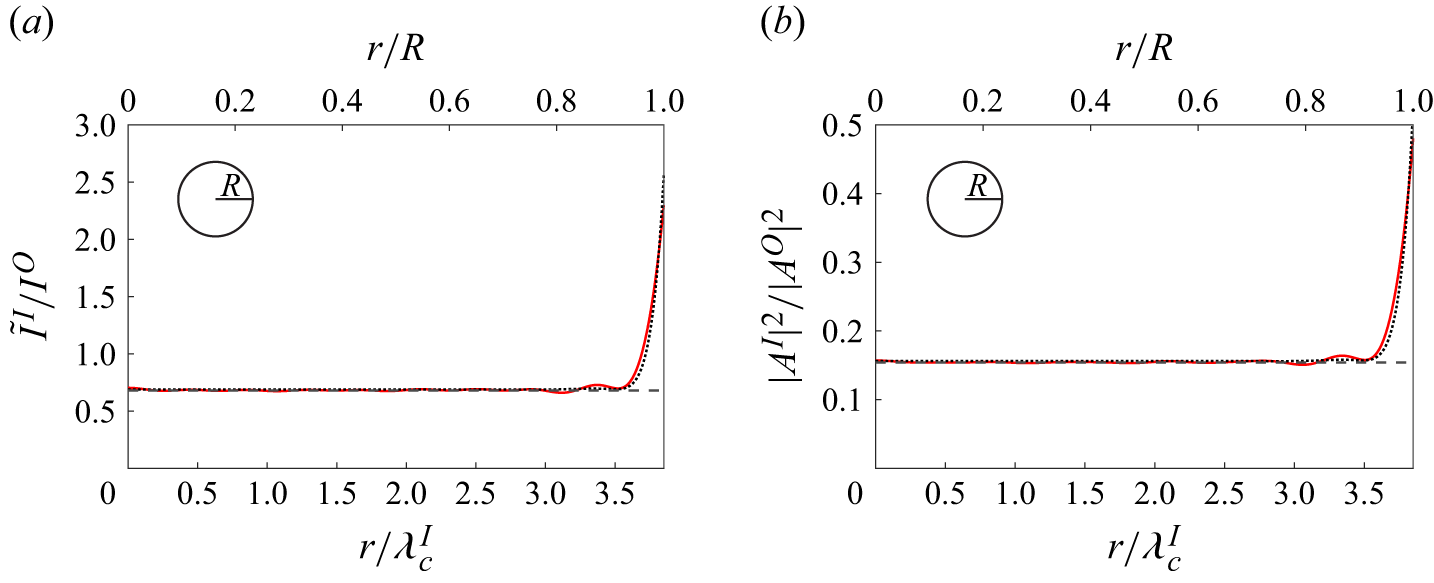
. We plot the radial cross-sections of both intensity (figure 3
a) and squared amplitude (figure 3
b) for a moderately large (
 $k^{I}R = 24$
) ice sheet in an isotropic incident wave field. The radial cross-section is not a function of azimuthal angle
 $\theta$
since the geometry and incident wave forcing are axisymmetric.
Radial distribution of (a) intensity and (b) squared amplitude for a circular ice sheet with
 $k^I_c\ell _D = 0.86$
,
 $k^O_c \gamma = 0.074$
and
 $k^I_c R = 24$
. We show direct computational results (red,
 ),
 $I^I_b$
(
 $|A^I_b|^2$
) (black,
 ) and
 $I^I_e$
(
 $|A^I_e|^2$
) (black,
 ) in (a) (and (b)). Inset depicts cross-section.

In figure 3, the intensity and squared amplitude are uniform in the bulk of the ice sheet except within
 $\lambda ^I_c$
of the ice edge. In figure 3(a), the intensity in the bulk is
 $\tilde {I}^I/I^O\approx k^I/k^O$
in agreement with the asymptotic result (3.10). With
 $k^I/k^O\lt 1$
in this case, the intensity reduction is the consequence of total reflection for an angular range of incident waves propagating from open water into the ice sheet as explained in § 3. In figure 3(b), the value of the squared amplitude in the bulk agrees with the theoretical result (4.13). The reduction in squared amplitude includes the effect of total reflection in addition to the change in group speed between open water and ice-covered regions and the difference in wave energy due to the flexural response and inertial effects of the ice.
Intensity and squared amplitude are related through the definitions of intensity (3.3). In general,
 $I^I = \sum _j \rho \omega ^2 (1 + \gamma k^I_j)C_{g,j}^I |A^I_j|^2/(2k_j^I)$
where
 $j$
refers to all the roots of the dispersion relation at frequency
 $\omega$
. However, our definition applies for
 $\boldsymbol{x}\in S^I/S^I_e$
and, hence, contains only the propagating component. We use
 $\tilde {I}^I$
for
 $\boldsymbol{x}\in S^I$
in figure 3(a) to indicate that our definition contains only the propagating component and is not strictly valid in
 $S^I_e$
. To avoid this ambiguity of definition, we present results in terms of squared amplitude exclusively for the remainder of this work. Note that, while it may appear that figure 3(a) is identical to figure 3(b) with the y-axis rescaled, the ratio
 $(\tilde {I}^I/I^O)/(|A^I|^2/|A^O|^2)$
varies spatially, particularly near the ice edge. This results from the frequency dependence of (3.3) upon frequency averaging.
We now consider the relation (4.10) between the ice response to an isotropic incident wave field and the Green function as well as the validity of the approximation (4.11) where we assume that, locally,
 $G$
behaves like
 $G^\infty$
. We verify (4.10) by comparing the direct computation of
 $|A^I|^2$
for an incident isotropic wave field via (5.1) (shown in figure 3
b) to the direct computation of
 $\mathrm{Re}\{F G_z^*(\boldsymbol{x}',0;\boldsymbol{x}')\}$
which yields
 $|A^I_{\textit{GF}}|^2$
via (4.10). We find that
 $|A^I|^2 = |A^I_{\textit{GF}}|^2$
everywhere in the ice sheet, even near the edges, as expected. For instance, in figure 3(b),
 $|A^I_{\textit{GF}}|^2$
(not shown) is indistinguishable from the direct computational results. Note that, while here we have compared the two results for a case with a narrow-banded spectrum and
 $k^{I}R\gg 1$
, we have also verified that (4.10) applies for general
 $k^{I}R$
and does not require frequency averaging.
While, in general,
 $G$
must be computed numerically, we are interested in the applicability of (4.11) which assumes the local response of
 $G$
can be approximated by
 $G^\infty$
. This is validated in this case by showing that
 $|A^I_{\textit{GF}}|^2\approx |A^I_b|^2$
in the bulk of the ice sheet away from the edge. Since
 $|A^I|^2 = |A^I_{\textit{GF}}|^2$
everywhere, this claim is supported by figure 3(b) where
 $|A^I|^2\approx |A^I_b|^2$
except near the ice edge.
We remark that the frequency-averaging provided by the narrow-banded spectrum is necessary for
 $|A^I|^2$
(and
 $I^I$
) to be uniform within the bulk of the ice sheet. For monochromatic forcing,
 $|A^I|^2$
oscillates in the radial direction around
 $|A^I_b|^2$
with wavelength
 $\lambda ^I/2$
due to the plan form-dependent wave interference pattern. The oscillation amplitude depends on
 $k^I\ell _D$
. The interference pattern is sensitive to frequency such that the oscillations are suppressed for sufficiently large
 $\Delta k^{I}R$
. Therefore, a smaller bandwidth
 $\Delta k^I/k^I_c$
is necessary for effective frequency averaging as
 $k^I_cR$
increases.
Although there are few observations of the directional wave field in the MIZ, the conditions reported by Wadhams et al. (Reference Wadhams, Squire, Goodman, Cowan and Moore1988) are in line with the short-wavelength theoretical results. For instance, the wave field is observed to be isotropic, reaching isotropy within 1.2 km of the ice edge in Run C and within 0.6 km for waves propagating through a band of ice floes. The description of Run C reports a narrow-banded wind sea with peak frequency at approximately 0.3 Hz, corresponding to an open-water wavelength
 $\lambda ^O=17$
m, propagating through an ice field with typical floe diameter
 $\ell =80$
m. Although further data about the ice is not available to determine
 $\lambda ^I$
, this corresponds to
 $k^O\ell \approx 30$
, indicating that the short-wavelength regime can be applicable in a realistic MIZ. Lastly, the ice concentration is reported to be 70 % during Run C. Using phase-resolved simulations of the MIZ, Montiel et al. (Reference Montiel, Squire and Bennetts2016) show that the wide-spacing approximation is valid for an ice concentration of 70 %.
5.2. Edge correction to theoretical results in the short wavelength regime
We develop an edge correction to the theoretical results to approximate the increase in squared amplitude near the ice edge based on the insight that the edge effects are (mostly) agnostic to plan form for
 $k^I_c\ell \gg 1$
. We consider the squared amplitude
 $|A^I|^2$
as a function of edge-normal distance into the ice sheet
 $x_n$
. Previous sections have established that
 $|A^I|^2\approx |A^I_b|^2$
for
 $x_n\gtrsim \lambda ^I_c$
where
 $|A^I_b|^2$
is a function of
 $k^I_c\ell _D$
and
 $k^O_c\gamma$
, but not ice sheet plan form, for
 $k^I_c\ell \gg 1$
. Through direct computations of circular and rectangular (see § 6) ice sheets, we find that, generally,
 $|A^I|^2$
for
 $0\leqslant x_n\lesssim \lambda ^I_c$
is a function of
 $k^I_c\ell _D$
and
 $k^O_c\gamma$
, but not ice sheet plan form, for
 $k^I_c\ell \gg 1$
. Note that this is not the case in regions where the edge has high curvature, such as at sharp corners. For the rectangular ice sheet cases (§ 6) we consider, the corner behaviour affects pointwise quantities, such as maximum bending strain, but generally has a small effect on the spatial mean of squared amplitude, important for determining in-ice dissipation.
We derive an edge correction to the theoretical result
 $|A^I_e(x_n)|^2$
based on this insight. We assume that regions of the ice edge without high curvature can be approximated as a straight edge for
 $k^I_c\ell \gg 1$
. We then determine
 $|A^I_e(x_n)|^2$
using the eigenfunction matching method of Fox & Squire (Reference Fox and Squire1994) to solve for the deflection of a semi-infinite ice sheet subjected to isotropic incident waves. For a given
 $k^I_c\ell _D$
and
 $k^O_c \gamma$
, we first determine the free surface elevation in the semi-infinite ice sheet
 $\eta ^{SI}(x_n;\psi ^O)$
for an incident wave propagating from open water into ice with unit amplitude and incident angles
 $\psi ^O\in [-\pi /2,\pi /2]$
. We also calculate
 $\eta ^{SI}(x_n;\theta ^I)$
for an incident wave propagating from ice into open water with amplitude
 $A^I_b$
and incident angles
 $\theta ^I\in [-\pi /2,\pi /2]$
. This requires a straightforward modification to the method of Fox & Squire (Reference Fox and Squire1994). We then angle and frequency average using
 \begin{equation} \langle |A^I_e(x_n)|^2 \rangle _\omega = \Biggl \lt \frac {1}{\pi }\left (\int _{-\pi /2}^{\pi /2}|\eta ^{SI}(x_n;\psi ^O)|^2 {\rm d}\psi ^O + \int _{-\pi /2}^{\pi /2} |\eta ^{SI}(x_n;\theta ^I)|^2{\rm d}\theta ^I\right ) \Biggr \gt _\omega . \end{equation}
Note that
 $\langle |A^I_e(x_n)|^2 \rangle _\omega \approx \langle |A^I_b|^2 \rangle _\omega$
for
 $x_n\gtrsim \lambda ^I_c$
.
 $I^I_e$
is obtained from (5.2) using the definition of intensity in ice (3.3b
).
Figure 3(b) compares the edge correction
 $|A^I_e|^2$
with direct computation of
 $|A^I|^2$
. We observe that
 $|A^I_e|^2$
recovers
 $|A^I_b|^2$
in the bulk of the ice sheet, as expected. At the ice edge
 $x_n=0$
,
 $|A^I_e|^2$
is within 0.05 of
 $|A^I|^2$
. Overall,
 $|A^I_e|^2$
is a good approximation of
 $|A^I|^2$
.
Note that the edge correction applies to ice sheets of general plan form. We show its applicability for rectangular ice sheets in § 6.
5.3. Range of validity of theoretical results with respect to the short-wavelength parameter
 $k^I\ell$

We consider the spatial mean of squared amplitude
 $\langle |A^I|^2\rangle _{\boldsymbol{x}}=(1/\mathcal{A})\int _{S_I}|A^I|^2{\rm d}S$
as a simple surrogate to evaluate the range of validity of the theoretical results and the edge correction with respect to
 $k^I_cR$
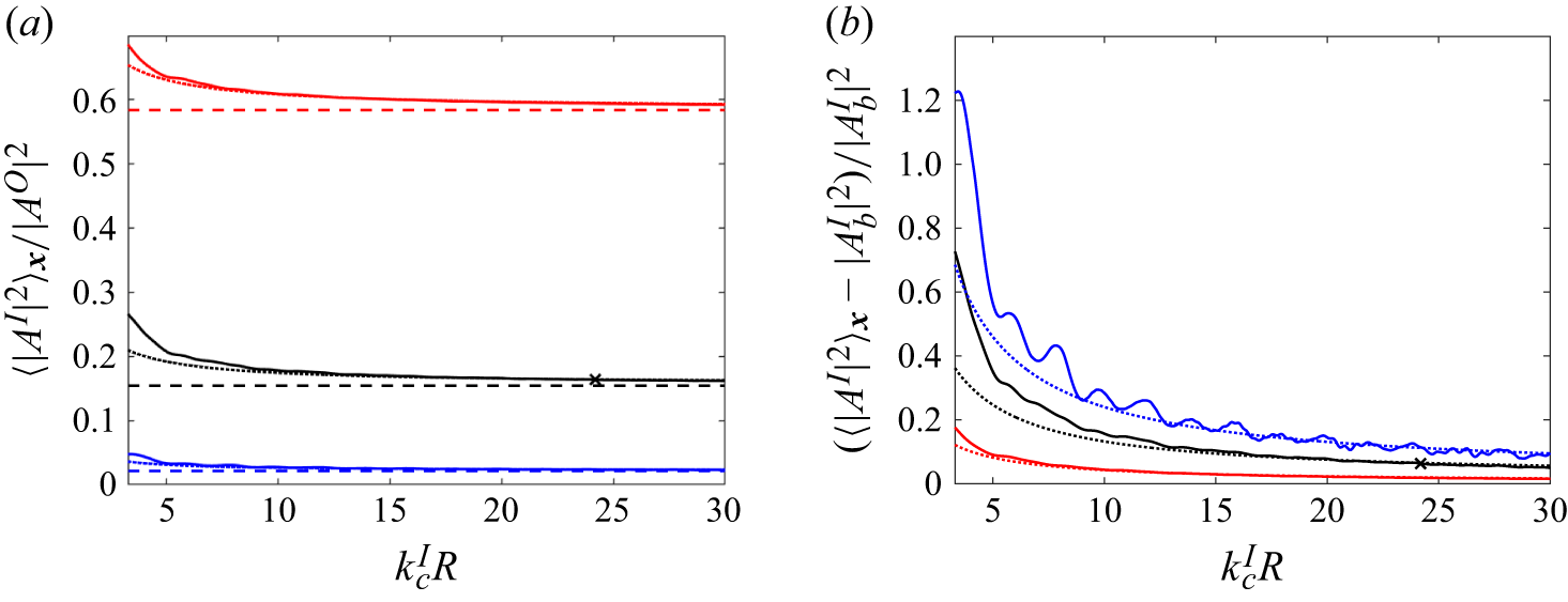
. Figure 4 displays
 $\langle |A^I|^2\rangle _{\boldsymbol{x}}$
as a function of
 $k^I_cR$
for three
 $(k^I_c\ell _D,k^O_c\gamma )$
pairs. These
 $(k^I_c\ell _D,k^O_c\gamma )$
pairs correspond to ice thicknesses
 $h=0.5$
,
 $1$
and
 $3.5$
m with the rest of the typical wave and ice parameters outlined at the start of § 5 held constant. We observe that
 $\langle |A^I|^2\rangle _{\boldsymbol{x}}$
approaches
 $|A^I_b|^2$
as
 $k^I_cR$
increases with a difference of less than 0.01 at
 $k^I_cR = 25$
for each ice thickness in figure 4(a).
Spatial mean of squared amplitude in circular ice sheet, normalised by (a)
 $|A^O|^2$
or (b)
 $|A^I_b|^2$
, for
 $(k^I_c \ell _D,k^O_c \gamma )=(0.56,0.028)$
(red),
 $(0.86,0.074)$
(black) and
 $(1.19, 0.26)$
(blue). We display direct computational results (
 ),
 $\langle |A^I_e|^2\rangle _{\boldsymbol{x}}$
(
 ) and
 $|A^I_b|^2$
(
 ) (in (a) only). Here
 corresponds to figure 3.

We can understand
 $\langle |A^I|^2\rangle _{\boldsymbol{x}}$
as the area-weighted average of
 $|A^I_b|^2$
and edge effects contained to
 $\mathcal{A}_e = \lambda ^I_cP$
, the area of
 $S_e^I$
, where
 $P$
is the perimeter of the ice sheet. From § 5.2, we know that the amplitude of edge effects remains constant as
 $k^I_cR$
varies which we denote as
 $\mathbb{C}$
. The area-weighted average can then be expressed as
 $\langle |A^I|^2\rangle _{\boldsymbol{x}} = (|A^I_b|^2 (\mathcal{A} - \mathcal{A}_e) +\mathbb{C}\mathcal{A}_e)/\mathcal{A} = |A^I_b|^2 + \tilde {\mathbb{C}}/(k^I_cR)$
, where
 $\tilde {\mathbb{C}}$
absorbs additional constants.
While this simple argument reveals that the edge effects decay with the inverse of
 $k^I_cR$
, we can use the edge correction to capture the leading-order effect, i.e. determine
 $\tilde {\mathbb{C}}$
. We make a theoretical prediction of
 $\langle |A^I|^2\rangle _{\boldsymbol{x}}$
by using the one-dimensional function
 $|A^I_e(x_n)|^2$
to form a two-dimensional surface of revolution
 $|A^I_e(\boldsymbol{x})|^2$
with
 $x_n=0$
along the circumference. We compare the theoretical prediction
 $\langle |A^I_e(\boldsymbol{x})|^2\rangle _{\boldsymbol{x}}$
with the direct computational result in figure 4 and find that
 $\langle |A^I_e(\boldsymbol{x})|^2\rangle _{\boldsymbol{x}}$
is a good approximation of
 $\langle |A^I|^2\rangle _{\boldsymbol{x}}$
for
 $k^I_cR\gtrsim 4\pi$
. At
 $k^I_cR=4\pi$
,
 $\mathcal{A}_e=3\mathcal{A}/4$
, so edge effects are important over most of the area. As a result, we expect the assumptions underlying the edge correction to no longer apply for
 $k^I_cR\lt 4\pi$
. The surprisingly good performance of the theoretical prediction also suggests that approximating the Green function for general plan form with the infinite-ice Green function remains valid even when
 $\mathcal{A}_e$
is comparable to
 $\mathcal{A}$
.
We include results for multiple
 $k^I_c\ell _D$
where
 $\ell _D = (D/(\rho g))^{1/4}$
in figure 4 to show that the theoretical result as well as the edge correction are applicable over a wide range of ice stiffnesses. Figure 4(a) shows that
 $|A^I_b|^2$
decreases for increasing ice thickness
 $h$
or elastic modulus
 $E$
, and that the highest
 $k^I_c\ell _D$
result is closest to
 $|A^I_b|^2$
for the entire range of
 $k^I_cR$
. This is because the amplitude of the edge effects
 $(|A^I(r=R)|^2-|A^I_b|^2)$
generally decreases as
 $k^I_c\ell _D$
increases. In figure 4(b), we normalize the results of figure 4(a) with respect to
 $|A^I_b|^2$
to enable comparison between different
 $k^I_c\ell _D$
. The results approach zero (corresponding to
 $|A^I_b|^2$
) in order of increasing
 $k^I_c\ell _D$
, opposite the trend in figure 4(a). This is because the amplitude of the edge effects, normalised by
 $|A^I_b|^2$
, generally increases as
 $k^I_c\ell _D$
increases. Note that the oscillations in the highest
 $k^I_c\ell _D$
result are due to the plan form-specific interference pattern mentioned in § 5.1 which are not totally suppressed for the selected bandwidth.
Figure 4(b) shows that both
 $k^I_cR$
and
 $k^I_c\ell _D$
are important to the range of validity of the theoretical results. This is indicative of the three relevant length scales of the problem:
 $k^I_c$
,
 $\ell _D$
and
 $\ell$
. We explore the interplay between these length scales in more depth in § 5.4.
5.4. Role of ice stiffness in predicting wave intensity in ice
Up to this point, we have mainly considered the short-wavelength regime (
 $k^I_cR\gg 1$
) where both theoretical results are applicable. However, it turns out that
 $|A^I|^2\approx |A^I_b|^2$
away from the ice edges even for
 $k^I_c\ell =O(1)$
when
 $\ell /\ell _D\gg 1$
. We depict the parameter space of the three dimensionless parameters
 $k^{I}_{c}R$
,
 $k_c^I\ell _D$
and
 $R/\ell _D$
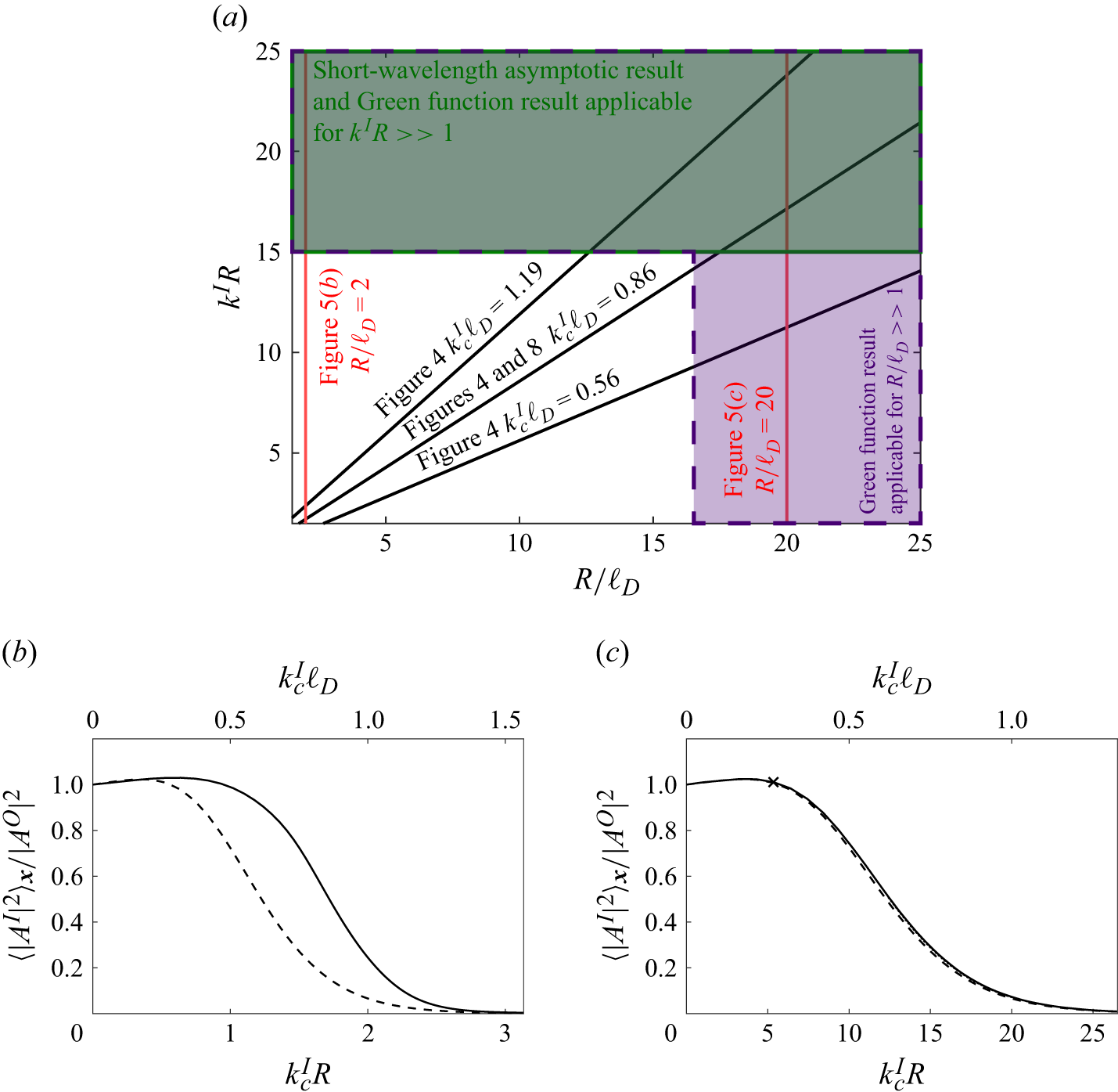
in figure 5(a) for a circular ice sheet with radius
 $R$
as an example. We also indicate how the various figures in this work cover different areas of the regime map. With
 $R/\ell _D$
on the abscissa and
 $k^I_cR$
on the ordinate, contours of constant
 $k_c^I\ell _D$
extend radially from the origin and increase in the anticlockwise direction.
We reiterate that the theoretical results apply when
 $k^I_c R\gg 1$
as evident in figure 4. Conversely, it is also clear in figure 4 that the theoretical results do not apply when both
 $k^I_cR$
and
 $R/\ell _D$
are
 $O(1)$
, corresponding to the lower left-hand quadrant of figure 5(a).
In figures 5(b) and 5(c), we plot
 $\langle |A^I|^2\rangle _{\boldsymbol{x}}$
as a function of
 $k^I_cR$
for constant
 $R/\ell _D$
to demonstrate the role of
 $R/\ell _D$
. In these figures, ice stiffness
 $k^I_c\ell _D$
is no longer constant but varies with
 $k^I_cR$
. At the y-axis,
 $k^I_cR = k^I_c\ell _D=0$
and we recover the long-wave limit where
 $\langle |A^I|^2\rangle _{\boldsymbol{x}}=|A^O|^2$
. In the other limit where
 $k^I_c\ell _D\gg 1$
,
 $\langle |A^I|^2\rangle _{\boldsymbol{x}}$
approaches zero as the ice sheet behaves as a rigid body. Figure 5(b) further supports that the theoretical results do not apply when
 $k^I_cR$
and
 $R/\ell _D$
are
 $O(1)$
since the computational results depart significantly from
 $|A^I_b|^2$
for
 $0.5\lesssim k^I_cR\lesssim 2.5$
. However, in figure 5(c) for
 $R/\ell _D = 20$
, the ice response is found to agree with
 $|A^I_b|^2$
for
 $k^I_cR = O(1)$
, i.e. the lower right-hand quadrant of figure 5(a), as well as for
 $k^I_cR \gg 1$
. We remark that
 $\langle |A^I_e|^2\rangle _{\boldsymbol{x}}$
is also plotted in figure 5(c) for
 $k^I_cR\gt 2\pi$
and is visually indistinguishable from the computed ice response.
We can use the Green function result to explain why
 $|A^I|^2\approx |A^I_b|^2$
also applies for
 $k^I_cR=O(1)$
when
 $R/\ell _D\gg 1$
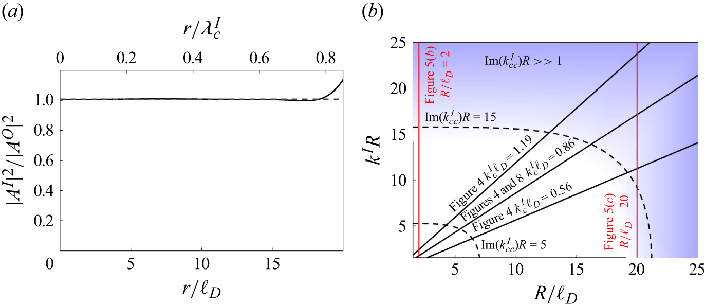
. Figure 6(a) displays the radial cross-section of
 $|A^I|^2$
for
 $k^I_cR = 5.35$
and
 $R/\ell _D = 20$
. As in § 5.1, we first validate that
 $|A^I|^2=|A^I_{\textit{GF}}|^2$
everywhere in the ice sheet. We then show that (4.11) is valid in the bulk of the ice sheet by showing that
 $|A^I_{\textit{GF}}|^2 \approx |A^I_b|^2$
, or, equivalently,
 $|A^I|^2 \approx |A^I_b|^2$
away from the ice edge in figure 6(a). While the SWA result does not apply to this case, the more general Green function result explains the observed behaviour.
(a) Regime map relating
 $R/\ell _D$
,
 $k^I_cR$
and
 $k^I_c\ell _D$
where regions with solid green border and dashed purple border indicate approximate range of validity for both SWA and Green function result and Green function result only, respectively. Spatial mean of squared amplitude in circular ice sheet for (b)
 $R/\ell _D = 2$
and (c)
 $R/\ell _D = 20$
. We display direct computational results (
 ) in (b) and (c),
 $|A^I_b|^2$
(
 ) in (b) and (c), and
 $\langle |A^I_e|^2\rangle _{\boldsymbol{x}}$
(
 ) in (c). In (c),
denotes the specific geometry of figure 6(a).

Figure 5. Long description
The image contains three panels labeled (a), (b), and (c). Panel A: A regime map graph showing the relationship between kR and R/vD. The x-axis is labeled R/vD and the y-axis is labeled kR. The graph includes regions with solid green borders and dashed purple borders indicating the range of validity for both short-wavelength asymptotic (SWA) and Green function results, and Green function results only, respectively. Several lines are plotted for different values of kc vD. Panel B: A line graph showing the spatial mean of squared amplitude in a circular ice sheet for R/vD = 2. The x-axis is labeled kcR and the y-axis is labeled <|A|^2>x/<|A0|^2>. The graph includes two lines, one solid and one dashed, representing different computational results. Panel C: A line graph showing the spatial mean of squared amplitude in a circular ice sheet for R/vD = 20. The x-axis is labeled kc vD and the y-axis is labeled <|A|^2>x/<|A0|^2>. The graph includes two lines, one solid and one dashed, representing different computational results. The solid line in Panel C denotes a specific geometry.
(a) Radial distribution of squared amplitude for a circular ice sheet with
 $k^I_c\ell _D = 0.27$
,
 $k^O_c\gamma = 0.016$
,
 $R/\ell _D = 20$
and
 $k^I_cR = 5.35$
. We display direct computational results (
 ) and
 $|A^I_b|^2$
(
 ). (b) Regime map from figure 5(a) where shaded blue region indicates the edge-affected region is much smaller than the total area,
 $\mathrm{Im}\{k^I_{cc}\}R\gg 1$
.

While the explanation above describes the response away from the edge-affected region, it does not explain why this region is small even for
 $k^I_cR=O(1)$
when
 $R/\ell _D\gg 1$
. We can understand this by recognizing that the edge effects are related to the complex-valued roots of the flexural-gravity dispersion relation:
 $\omega ^2 = (gk^I + D(k^I)^5/\rho )/(1+\gamma k^I)$
. These complex-valued modes exhibit oscillatory decay with distance from the ice edge with the real and imaginary parts determining the wavelength and
 $e$
-folding length respectively. We find that the imaginary part of the complex-conjugate wavenumber, denoted
 $\mathrm{Im}\{k^I_{cc}\}$
, generally determines the length scale of the edge layer. Consequently, when
 $\mathrm{Im}\{k^I_{cc}\}R \gg 1$
, the edge-affected layer is much smaller than the bulk of the ice sheet where
 $|A^I|^2 \approx |A^I_b|^2$
. We show representative contours of constant
 $\mathrm{Im}\{k^I_{cc}\}R$
in figure 6(b).
For
 $k^I_c\ell _D \lt 1$
,
 $\mathrm{Im}\{k^I_{cc}\}\sim 1/\ell _D$
. This is evident in figure 6(a) where the edge effects extend
 $O(\ell _D)$
from the ice edge (which is equivalent to
 $O(0.1\lambda ^I_c)$
). On the other hand, for
 $k^I_c\ell _D \gt 1$
,
 $\mathrm{Im}\{k^I_{cc}\}\sim k^I_c$
. This explains why the theoretical result is valid for
 $k^I_cR\gg 1$
when
 $k^I_c\ell _D \gt 1$
and for
 $R/\ell _D\gg 1$
when
 $k^I_c\ell _D \lt 1$
. Note that
 $k^I_cR\gg 1$
and
 $R/\ell _D\gg 1$
are equivalent when
 $k^I_c\ell _D = 1$
. This corresponds with what we see in figure 3 where the edge effects extend
 $O(\lambda ^I_c\approx \ell _D)$
from the edge.
For typical physical parameters and 0.5 m-thick ice,
 $\ell _D \approx 9$
m, and
 $\ell$
ranges from
 $O(1\,\mathrm{m})$
close to the edge of the MIZ to
 $O(1\,\mathrm{km})$
in the interior. Here
 $\ell /\ell _D\gg 1$
is therefore likely to apply to an appreciable portion of ice sheets in the MIZ.
6. Illustrative results for ice sheets of rectangular plan form
We consider rectangular ice sheets of different aspect ratio to show that the theoretical results and the edge correction are agnostic to ice sheet plan form (away from the corners). We demonstrate that the ice sheet geometry does have some effect on the asymptotic approach to
 $|A^I_b|^2$
through its perimeter to area ratio. We use the method of Porter (Reference Porter2019) which combines Fourier and Rayleigh–Ritz methods to determine the ice sheet deflection of a rectangular ice sheet for a unidirectional and monochromatic incident wave. We then perform frequency and angle averaging using (5.1). After performing convergence testing with respect to
 $\langle |A^I|^2\rangle _{\boldsymbol{x}}$
for rectangular ice sheets with aspect ratio
 $AR=1$
and 4, we use 128 plate modes, 128 beam modes per plate mode,
 $N_\theta = 64$
and
 $N_\omega = 9$
. We expect the numerical error to be less than 1 % for this selection of parameters.
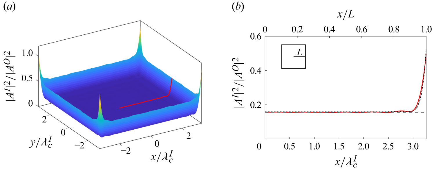
Squared amplitude (a) surface and (b) horizontal cross-section for square ice sheet with side length
 $2L$
,
 $k^I_c\ell _D=0.86$
,
 $k^O_c\gamma =0.074$
and
 $k_c^IL = 21$
(
 $k_c^I\ell = 41$
). We show direct computational results in (a) and (b) (red,
) as well as
 $|A^I_b|^2$
(black,
 ) and
 $|A^I_e|^2$
(black,
 ) in (b).

In figure 7, we show the spatial variation of squared amplitude for a square ice sheet (
 $AR=1$
) with side length
 $2L$
(
 $=\ell$
) for a moderately large
 $k^IL= 21$
. Figure 7(b) shows that
 $|A^I|^2\approx |A^I_b|^2$
more than a wavelength from the ice edge as expected. Note that the same parameters
 $k^I_c\ell _D = 0.86$
and
 $k^O_c\gamma = 0.074$
are considered in both figure 3 for a circular ice sheet and in figure 7 for a square ice sheet, so
 $|A^I_b|^2$
is the same as well.
The edge correction is also applicable to rectangular ice sheets. The procedure to find
 $|A^I_e(x_n)|^2$
is identical to that described in § 5.2. However, the process to find the two-dimensional function
 $|A^I_e(\boldsymbol{x})|^2$
is modified for the different geometry. We determine
 $|A^I_e(\boldsymbol{x})|^2$
by reflecting
 $|A^I_e(x_n)|^2$
to create generating curves matching the length and width of the rectangle. We use these curves to generate two surfaces – one with the edge correction applied to the top and bottom edges and the other to the right- and left-hand edges. We sum these two surfaces and subtract
 $|A^I_b|^2$
to find
 $|A^I_e(\boldsymbol{x})|^2$
. Note the edge correction is not applicable at corners where the assumption of a locally straight edge does not apply.
In figure 7(b), we see the edge correction captures the edge effects well with
 $|A^I_e|^2$
only slightly exceeding the direct computational results. By comparing figures 3(b) and 7(b) for the circular and the square ice sheet, we see that the edge effects are very similar. At the corners, the squared amplitude is greater than elsewhere along the edge as seen in figure 7(a).
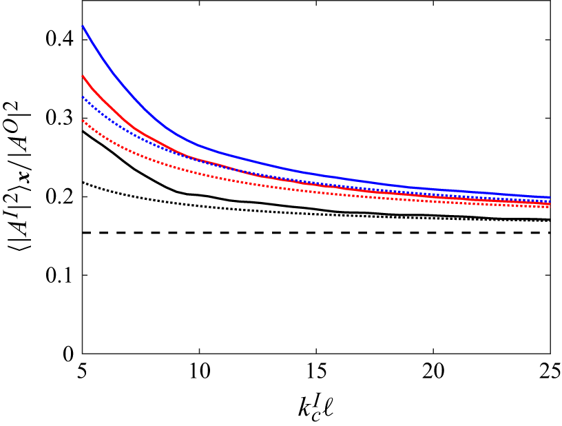
Spatial mean of squared amplitude for circular (black), square (red) and rectangular (aspect ratio of 4) (blue) ice sheets for
 $k^I_c\ell _D = 0.86$
,
 $k^O_c\gamma = 0.074$
. We show direct computational results (
 ),
 $|A^I_b|^2$
(
 ) and
 $\langle |A^I_e|^2\rangle _{\boldsymbol{x}}$
(
 ).

In figure 8, we show that
 $\langle |A^I|^2\rangle _{\boldsymbol{x}}$
approaches
 $|A^I_b|^2$
for circular, square and rectangular ice sheets but at different rates for the same
 $k^I_c\ell _D$
and
 $k_c^O\gamma$
. To compare different geometries, we plot against
 $k^I\ell$
where
 $\ell = \sqrt {\mathcal{A}}$
and
 $\mathcal{A}$
is the ice sheet area, such that each geometry has the same area at a given
 $k^I\ell$
. Here
 $\ell = \sqrt {\pi }R$
for a circular ice sheet and
 $\ell = 2L$
for a rectangular ice sheet. We find the circular ice sheet results approach
 $|A^I_b|^2$
fastest with increasing
 $k^I_c\ell$
, followed by the square and then the rectangle. The theoretical results with the edge correction
 $\langle |A^I_e|^2\rangle _{\boldsymbol{x}}$
for the different plan forms approach
 $|A^I_b|^2$
in the same order and are generally good approximations of the direct computational results for
 $k^I_c\ell \gtrsim 20$
(which is approximately equivalent to the range
 $k^I_cR\gtrsim 4\pi$
from § 5.3).
For simple geometries, we can heuristically explain the order of approach by revisiting the reasoning presented in § 5.3 for why
 $\langle |A^I|^2\rangle _{\boldsymbol{x}}$
approaches
 $|A^I_b|^2$
for
 $k^I_c\ell \gg 1$
. Recalling the area-weighted average,
 $\langle |A^I|^2\rangle _{\boldsymbol{x}} = (|A^I_b|^2 (\mathcal{A} - \mathcal{A}_e) +\mathbb{C}\mathcal{A}_e)/\mathcal{A} =|A^I_b|^2 + (\mathbb{C} - |A^I_b|^2) \lambda ^I_cP/\mathcal{A}$
where we have used
 $\mathcal{A}_e = \lambda ^I_cP$
. The perimeter to area ratio
 $P/\mathcal{A}$
appears in the second term. Here
 $P/\mathcal{A}$
is least for a circle followed by a square and then a rectangle with aspect ratio of 4 in agreement with the order observed in figure 8.
We note that we also observe results (not shown) similar to figures 5(b) and 5(c) for square and rectangular ice sheets. This supports that the findings for
 $\ell /\ell _D\gg 1$
are not unique to a circle.
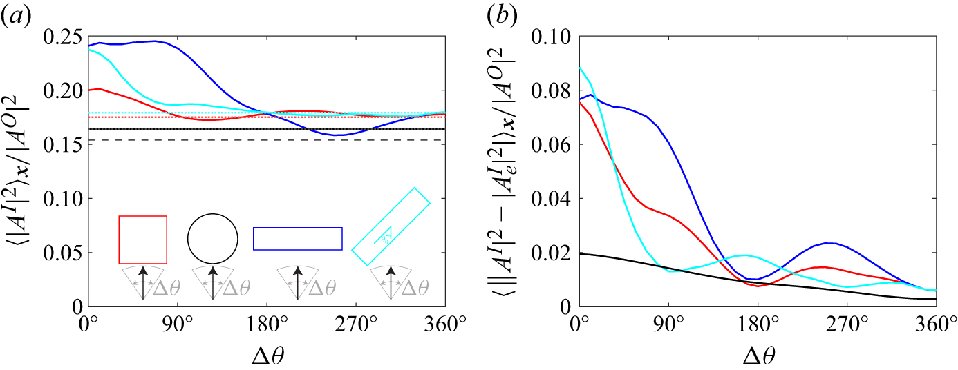
Spatial mean of (a) squared amplitude and (b) absolute difference between squared amplitude from computation and theory with edge correction, as a function of directional spread
 $\Delta \theta$
for circular (black), square (red) and rectangular (aspect ratio of 4) ice sheets for
 $\theta _0=0^\circ$
(blue), and
 $45^\circ$
(cyan); for
 $k^I_c\ell _D = 0.86$
,
 $k_c^O\gamma = 0.074$
and
 $k_c^I\ell = 43$
. In (a), we show direct computational results (
),
 $|A^I_b|^2$
(
) and
 $\langle |A^I_e|^2\rangle _{\boldsymbol{x}}$
(
).

7. Comments on the effect of deviation from an isotropic incident wave field
It is of interest to show how the ice response deviates from theoretical predictions when ambient wave field isotropy is not strictly satisfied. When the ambient waves are confined in a (top hat) directional spread of
 $\theta \in [\theta _0-\Delta \theta /2,\theta _0+\Delta \theta /2]$
, figure 9 shows the deviation from theoretical prediction as a function of
 $\Delta \theta$
, ice floe plan form geometry, and
 $\theta _0$
.
We see that the isotropic theory performance is generally dependent on plan form geometry/aspect ratio and
 $\theta _0$
, as expected, and the theory is surprisingly still reasonably useful even when
 $\Delta \theta$
decreases towards
 $\sim 180^\circ$
. The circle result is a special case where
 $\langle |A^I|^2\rangle _{\boldsymbol{x}}$
does not vary with
 $\Delta \theta$
and is in close agreement with
 $\langle |A^I_e|^2\rangle _{\boldsymbol{x}}$
(figure 9
a). Heuristically, this occurs because the angle averaging effect arises from the circular geometry rather than the isotropic wave field. However, figure 9(b), which plots the spatial mean of the absolute difference between the theory and computational results, shows that the squared amplitude is not axisymmetric and uniform within the bulk as in figure 3 for all
 $\Delta \theta$
, but rather smoothly approaches the isotropic prediction as
 $\Delta \theta$
increases.
8. Conclusion
We set out to determine the wave intensity within a floating ice sheet of general plan form in the MIZ given the wave intensity in the surrounding open water. Wave intensity is the angular distribution of wave energy flux and is proportional to squared directional wave amplitude. We consider the incident wave spectrum in the open water surrounding the ice sheet to have narrow bandwidth, typical of the realistic ocean environment, and to be isotropic due to multiple scattering by the other ice sheets in the MIZ. We assume sufficient spacing between the ice sheets so we can consider a single ice sheet in isolation with negligible near-field interaction. We consider the ice sheet to behave as a thin, uniform elastic plate without dissipation. We identify three key length scales in this problem: the characteristic length of the ice sheet plan form
 $\ell$
, the wavenumber in ice at the centre of the spectrum
 $k^I_c=2\pi /\lambda ^I_c$
and the flexural-gravity length scale
 $\ell _D$
.
We derive a SWA result in § 3 under the assumption that
 $k^I_c\ell \gg 1$
and the wave fields within the ice-covered region and in the surrounding open water are uniform and isotropic. We obtain that the ratio of intensity in ice to that in open water is equal to the ratio of the wavenumber in the respective regions (see (3.10)). Typically, the wavenumber in ice is less than in open water, so the intensity in ice is reduced compared with the surrounding open water. This result is agnostic to the ice sheet plan form, making it useful for the irregular ice shapes of the MIZ.
In § 4, we derive a more general result using a Green function which describes the response to harmonic point forcing of the ice sheet. We derive a result relating the ice response in an isotropic wave field to the Green function
 $G$
evaluated at its source point (see (4.10)). In general,
 $G$
must be determined numerically to satisfy the ice edge boundary conditions. However, away from the ice edge,
 $G$
can be locally approximated by
 $G^{\infty }$
(see (4.11)), where
 $G^{\infty }$
is the Green function for an ice sheet of infinite extent, which has a closed-form expression. For
 $k^I_c\ell \gg 1$
, this approximation is valid everywhere except the ice edge, so the Green function result (4.14) recovers the SWA result (3.10). In addition to the SWA limit, we show that the Green function result also applies for
 $\ell /\ell _D\gg 1$
regardless of
 $k^I_c\ell$
.
In § 5, we describe direct computations of the ice response of a circular ice sheet in an isotropic wave field to elucidate the range of validity of the theoretical results. We first consider cases where
 $k^I_c\ell \gg 1$
. We show that the squared amplitude in the ice sheet away from the edges is uniform and matches the theoretical results. Within a wavelength inward from the edge, the squared amplitude exceeds the uniform value in the bulk. We find this edge effect is not a function of the ice geometry and is well approximated by an edge correction to the value in the bulk where the edge is treated locally as a semi-infinite ice sheet. With the edge correction, the theoretical results agree well with the ice response for
 $\ell \gtrsim 3\lambda ^I_c$
. We also consider cases with
 $\ell /\ell _D\gg 1$
, for a range of
 $k^I_c\ell =O(1)$
, where the Green function result (but not SWA) apply. We show that the intensity is uniform and equal to the wavenumber ratio predicted by the theory, except within approximately
 $\ell _D$
of the ice edge.
We evaluate the range of validity of the approximation made in the Green function result by comparing direct computations of the Green function for a circular ice sheet with the closed-form expression for the infinite-ice Green function. We find the approximation is valid except within the edge-affected region. We recognize that the spatial extent of the edge-affected region scales with the imaginary part of the complex-valued roots of the flexural-gravity dispersion relation, recovering both the
 $k^I_c\ell \gg 1$
and
 $\ell /\ell _D\gg 1$
regimes.
In § 6, we consider rectangular ice sheets of various aspect ratio to support that the theoretical results, including the edge correction, are agnostic to the ice sheet plan form. In § 7, we show that the theoretical predictions can be surprisingly robust even when the ambient wave field has not reached full isotropy, suggesting that the theory may be useful in a broader region within a typical MIZ.
As an initial effort, we have not considered dissipative effects on waves propagating in ice in this work. These effects include viscous dissipation at the fluid–ice interface as well as the viscoelastic response of the ice. The current findings should be applicable provided that the length scale over which significant dissipation occurs is greater than ice floe length scale
 $\ell$
.
Acknowledgements
The authors acknowledge the MIT Office of Research Computing and Data for providing HPC resources that have contributed to the research results reported within this paper. This research is supported financially by grants from the Office of Naval Research and MIT Sea Grant. M.W.P. was also supported by a MathWorks Fellowship during a portion of this work.
Declaration of interests
The authors report no conflict of interest.
 kcIℓD=0.86
 kcOγ=0.074
 kcIR=24
 IbI
 |AbI|2
 IeI
 |AeI|2
 |AO|2
 |AbI|2
 (kcIℓD,kcOγ)=(0.56,0.028)
 (0.86,0.074)
 (1.19,0.26)
 ⟨|AeI|2⟩x
 |AbI|2
 R/ℓD
 kcIR
 kcIℓD
 R/ℓD=2
 R/ℓD=20
 |AbI|2
 ⟨|AeI|2⟩x
 kcIℓD=0.27
 kcOγ=0.016
 R/ℓD=20
 kcIR=5.35
 |AbI|2
 Im{kccI}R≫1
 2L
 kcIℓD=0.86
 kcOγ=0.074
 kcIL=21
 kcIℓ=41
 |AbI|2
 |AeI|2
 kcIℓD=0.86
 kcOγ=0.074
 |AbI|2
 ⟨|AeI|2⟩x
 Δθ
 θ0=0∘
 45∘
 kcIℓD=0.86
 kcOγ=0.074
 kcIℓ=43
 |AbI|2
 ⟨|AeI|2⟩x


