

1. Introduction
Almost all countries of the world today have accepted the need to regulate economic activities in order to protect the environment. However, in many less developed countries (LDCs), we observe that there is usually a lot of resistance to the implementation of such policies, citing problems of unemployment. It is argued that since cleaner goods are typically more capital intensive, stringent environmental standards inflict a short-run employment loss in the LDCs. With markets already unable to absorb the total workforce, the loss of employment makes it politically difficult to continue with such regulations in a democratic country like India. However, it is universally accepted that an improvement in environmental quality improves the health of the workers and this increases their productivity. In this paper, we critically examine the impact of this productivity effect of an environmental standard on aggregate employment in a multi-sector general equilibrium framework of an open economy. We show that the productivity effect enhances the appeal of environmental standards as it increases the chances of employment expansion.
There have been a few studies that have analysed how environmental regulation affects employment. The ‘double dividend hypothesis’ which claims that environmental protection and social objectives like employment generation may go hand in hand has been hotly debated. The theoretical literature indicates that very restrictive conditions must be met for the recycling of environmental taxation to produce an increase in employment. In an empirical study, Morgenstern et al. (Reference Morgenstern, Pizer and Shih2002) examined the ‘jobs versus environment’ debate at the industry level for four heavily polluting industries: pulp and paper mills, plastic manufactures, petroleum refiners, and iron and steel mills of the USA. They showed that an increase in environmental spending does not cause a significant change in employment. The relationship between environmental protection and sectoral unemployment has been addressed in a Harris–Todaro framework in many papers. In a closed model, Daitoh (Reference Daitoh2003) analysed the effect of an increase in the pollution tax rate on manufacturing employment and urban unemployment. He argues that, while an increase in the pollution tax rate will lower the scale of production, reducing employment, it will also induce substitution between labour and the dirty input and that if the relative price-elasticity of relative demand for the manufactured good is sufficiently small, then the substitution effect will dominate and manufacturing employment will rise. Chao et al. (Reference Chao, Kerkvliet and Yu2000) found that, in a closed economy with sectoral unemployment, an increase in the preservation of raw materials leads to a rise in the urban unemployment ratio. However, in a small open economy, an increase in environmental protection does not result in additional domestic unemployment. These papers talk of sectoral employment only and not of aggregate employment in an open economy. This issue has been analysed by Wagner (Reference Wagner2005) and Sen and Acharyya (Reference Sen and Acharyya2007) who pointed out that, while environmental regulation has an adverse effect on aggregate employment as production shifts to cleaner and more capital intensive technology, there is also a corresponding increase in abatement activities which generate employment and may offset the initial loss.
None of the above papers takes into consideration the fact that environmental regulation may affect the health of the workers and hence labour productivity, and this can have a significant impact on employment. Only a few papers discuss the impact of environmental regulation on health and labour productivity. Chakrabarti and Mitra (Reference Chakrabarti and Mitra2005) observed that the health of the workers improved after environmental regulations were imposed in the lead-smelting sector in Calcutta, India. Williams (Reference Williams2002) analysed the case where an increase in environmental tax lowers pollution levels and improves the health of workers. The reduction in pollution directly increases the utility of consumers. At the same time, improved health increases labour productivity by reducing the time spent sick by a worker. This influences a person's labour–leisure decisions and affects labour supply. His paper, however, is limited to the supply side of the labour market only. Also, since the model is a full employment one, the ultimate effect of environmental regulation boils down to changes in wages.
In contrast to this supply-constrained model where the influence of the productivity effect comes through labour supply in a model with full employment, we consider the case where the productivity effect affects labour demand in a model of unemployment to study how an environmental standard affects aggregate employment. In particular, we show that, though the productivity effect initially lowers labour demand by lowering the labour requirement per-unit of production, aggregate employment may rise because the same productivity effect augments total production and makes production less capital intensive. In the end, aggregate demand for labour and consequently employment may well increase depending on the parametric configurations.
In this paper, we have focused on the impact of the productivity effect, direct and indirect, on the employment of unskilled labour. For this purpose, we consider a simple general equilibrium structure of a small open economy. The economy produces a set of final consumption goods that are traded with the rest of the world and a non-traded intermediate good. Among the traded goods, we distinguish between a composite of export and import goods that have no environmental implications whatsoever and an export good which degrades the environment when produced. The extent of pollution generated by this export good, which is not domestically consumed, varies according to its environmental quality. The environmental quality depends upon the intensity in which the non-traded intermediate good, a cleansing device for example, is used along with unskilled workers in the production of this dirty export good. Instead of assuming environmental quality of the export good to be exogenously given, we consider a profit-maximizing choice of such quality by the competitive producers. Also, as the producers face a resource constraint, there is a trade-off between the quantity of the dirty good that is being produced and its environmental quality (as a cleaner quality requires more of the cleansing input).
Since the pollution generated by the dirty export adversely affects the productivity of both unskilled and skilled workers, an imposition of an environmental standard improves their productivity. To begin with, the improvement in the productivity of unskilled workers reduces the demand for labour and employment as now the per-unit requirement of labour falls. However, the improvement in the productivity of the skilled workers increases the effective supply of skilled labour and hence allows an expansion of the intermediate (cleansing) sector and dirty export sector, generating some employment. In addition to this, the change in productivity changes factor prices which trigger substitution between factors and change output levels.
In the above set up, we show that in the presence of the productivity effect, a binding minimum environmental standard may raise aggregate employment, depending on the degree of substitutability of capital and skilled labour in the production of the intermediate cleansing device. However, if we ignore the productivity effect, the criteria for employment expansion narrows down substantially and the arguments in favour of the imposition of environmental standards lose their edge.
The rest of the paper is organized as follows. In section 2 we set out the basic model of environmental-quality selection of ‘dirty’ exports. Section 3 examines the effect of environmental-quality restrictions on aggregate employment and brings out the implications of productivity effects in this context. In section 4, we discuss some robustness issues by extending the basic analytical framework to include flexible input coefficients, examining the importance of the factor intensity assumptions made in the main text and considering a more general framework where the dirty good is produced using unskilled labour, capital and the intermediate cleansing good. Finally, in section 5, we conclude the paper.
2. The model
Consider a home country trading two goods, T and Z, with the rest of the world. Being a small open economy, the home country cannot influence the world price of these traded goods by varying its volume of trade. Traded good T is a composite of all those exports and import-competing goods that have no environmental impact whatsoever. Thus, T is a composite of clean traded goods. Good Z is a dirty export (and is not domestically consumed in the home country) in the sense that it generates pollution when produced. Such pollution, like toxic wastes and carbon dioxide emissions, causes health hazards at both the local and global level. The extent of environmental degradation or pollution emission during production is assumed to be dependent on the technique of production. That is, pollution declines with the relatively more intensive use of a cleansing device which is an intermediate good used in the production of the dirty good Z. We capture this variation in pollution by an index of environmental quality of Z, A∈ [0, Ā], which is observable by all.Footnote 1 A higher value of A means that Z is of a cleaner variety, that is, more intermediate cleansing good is used in the production of one unit of the Z. Ā denotes the cleanest variety that can be produced, given the state of technology. Such characterization of environmental quality as an attribute of the consumer good has been used by Arora and Gangopadhyay (Reference Arora and Gangopadhyay1995), Bansal and Gangopadhyay (Reference Bansal and Gangopadhyay2003) and Sen and Acharyya (Reference Sen, Acharyya and Khasnobis2002, Reference Sen and Acharyya2007).Footnote 2 Since a cleaner variety of Z uses more of the intermediate cleansing good, the per-unit intermediate good requirement of Z increases with the environmental quality. It is also assumed that the cleansing device generates diminishing returns. So,

where a ij is per-unit requirement of the ith input for production of the jth good:

The composite traded clean good T is taken to be the numeraire good in terms of which all other prices are expressed and is normalized to one. There are three primary factors of production: skilled labour (S), unskilled labour (L) and physical capital (K). The clean composite traded good T is produced by capital and unskilled labour, the dirty export good Z by the intermediate good and unskilled labour, and the intermediate good (or cleansing device) by capital and skilled labour. So, while T uses only two factors – capital and labour – the dirty export requires all three factors, either directly or indirectly.Footnote 3 The production technologies for the final traded goods are assumed to be Leontief or fixed coefficient technology.Footnote 4 Technology in producing the cleansing device (I), on the other hand, is assumed to permit substitution of physical capital by skilled labour and vice versa. The extent of such substitutability is measured by the factor substitution elasticity σI. All the product and factor markets are perfectly competitive. Skilled wage w S and the rate of return to capital r, both measured in terms of good T, are fully flexible such that the markets for skilled workers and physical capital clear. On the other hand, we assume a rigid (real) wage for unskilled labour which is too high to ensure full employment of unskilled workers. This assumption, which is not at odds with the labour market inflexibilities (such as minimum wage policy and trade union activities preventing wage competition among unemployed workers) in many developing countries and even in some of the European countries, is purpose specific. By such wage rigidity we generate an initial less-than-full-employment situation to create scope for analysing the employment implications of an environmental regulation.
For convenience we list below some of the variables to be used in the paper.
 :
fixed (real) unskilled wage
- r:
(real) rate of return to capital
- w S:
(real) skilled wage
- P Z* (A):
relative world price of Z of environmental quality A
- X j:
output of the jth good (j = T, Z, I)
- X Id:
quantity demanded of the intermediate good
- :
stock of domestic capital
- L e:
level of aggregate employment of unskilled labour
- μj:
unskilled-labour productivity elasticity in sector j (j = Z, i) and
- μS:
skilled-labour productivity elasticity in sector I.
 :
 :
The other notations of the model will be defined as they appear.
This paper focuses on the benefits of using the cleansing device. So, while the imposition of a minimum environmental standard increases the average cost of the dirty good, it generates a positive social externality, that is, it improves the health of the workers in all the sectors. This improves their labour productivity. So, an improvement in environmental quality improves the marginal productivity of both skilled and unskilled workers at a constant rate.Footnote 5 That is,

The extent of such productivity improvement is measured by the elasticity of marginal productivity defined below:


We also assume in our analysis that the dirty export good Z is unskilled-labour intensive compared to the composite traded good T. That is,

where λLj = a LjX j/L e; λKj = a KjX j/K.
This assumption is not unreasonable because cleaner goods are generally more capital intensive.Footnote 6
Finally, we assume that buyers in the rest of the world value the environment and this is reflected in their higher willingness-to-pay for a cleaner variety of good Z. Thus, our small open economy faces the following price-quality schedule in the world market:

Two comments are warranted at this point. First of all, there is some empirical evidence that environmentally friendly or eco-labelled goods command a significant price premium (Irland, Reference Irland1993; Forsyth et al., Reference Forsyth, Haley and Kozak1999; Nimon and Beghin, Reference Nimon and Beghin1999). Nimon and Beghin (Reference Nimon and Beghin1999), for example, observe that ‘eco-labelled apparel items command a price premium of about 30 per cent relative to comparable conventional apparel items’ in the US markets. Mattoo and Singh (Reference Mattoo and Singh1994) and Upton and Bass (Reference Upton and Bass1996) also observe that 80 per cent of consumers in UK and Canadian markets are willing to pay more for environmentally friendly goods. Second, the price premium for environmentally friendly goods, and the continuity assumption in (5), enable us to determine the environmental quality of good Z as a profit-maximizing choice of the competitive producers in the home country instead of assuming it as exogenously given. Of course, as we will show later, for our main results this will not be as important as the direct productivity effect, but the extent of price premium paid by foreign buyers will definitely make the condition for an increase in aggregate employment less stringent.
Given the above set of assumptions, the set of equations (6)–(17) specifies the analytical structure of the home economy. Since the three sectors are perfectly competitive, price equals marginal (or unit) cost for any given environmental quality, A. The zero-profit conditions in these three sectors are given by:



Now, for any given price of the intermediate good and the fixed unskilled wage, at the profit-maximizing environmental quality A 0, the marginal-benefit from an improvement in environmental quality equals marginal-costFootnote 7

The net benefit from environmental quality that accrues to the Z sector includes the higher price commanded by the cleaner variety and the improvement in unskilled-labour productivity in the Z sector. The marginal benefit from improvement in environmental quality is:

The average cost of production of one unit of Z depends on the quality of Z that is being produced, the wage rate of unskilled labour and the price of the cleansing good,

Though the cost of production of a cleaner variety is more as it requires more intermediate good, the increase in cost is somewhat tempered by the improvement in labour productivity. So, marginal cost of environmental-quality improvement (net of the productivity gain) is

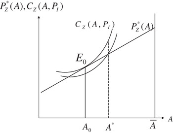
Thus, the marginal condition where marginal benefits equal marginal costs is given by equation (9). Given the price-quality schedule (5), the zero-profit condition (6) and the marginal condition (9) together determine the equilibrium environmental quality A 0 and P I. This profit-maximizing choice of the environmental quality of export good Z is illustrated in figure 1. The equilibrium can be represented by point E 0 in figure 1 where the price line is tangent to the cost curve and as in equation (9). The C Z (A, P I) curve is increasing and convex by the properties assumed in (1), while the P Z* (A) line captures the foreign willingness-to-pay as defined in (3). At the tangency point between the two, both the zero-profit condition (6) and the marginal condition (9) are satisfied and, accordingly, the environmental quality A 0 and the price of the (non-traded) intermediate good are determined.
Choice of environmental quality

Although the traded sectors have fixed coefficient production functions, there can be substitution between skilled labour and capital in the intermediate cleansing sector, given any A. So, the input coefficients of the intermediate good are assumed to depend on the ratio of factor prices,
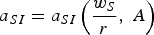

The substitutability of physical capital by skilled labour (for any given level of production) is captured by the factor substitution elasticity, σI, defined as

As the intermediate good is a non-traded good used only in the production of Z, its demand is determined by the amount of Z that is produced,

The fixed supply of skilled labour, which is specific to the production of I, however, places a constraint on the supply of I, given a w s/r ratio. An increase in the ratio prompts substitution of skilled labour with capital and the per-unit requirement of skilled labour falls, enabling an increase in the production of I,

Thus, given w s/r, the output of I imposes a trade-off between the quantity and environmental quality of Z as shown in (13). As capital is used in the T and I sectors, the full employment condition of capital (15) determines the volume of output of the traditional sector in the economy,Footnote 8

The level of employment of unskilled labour is then

The demand, and hence the aggregate employment of unskilled labour, depends on the output levels of the traded goods and the environmental-quality level of good Z. The environmental quality directly affects the employment adversely through the productivity effect. An improvement in A raises the productivity of labour, and so less labour is required to produce the same level of output. So, demand for labour, at constant output, is lower. But this, as we will show in the next section, is only the direct effect. The change in the productivity of skilled and unskilled labour also affects the scale of production of T and Z, which in turn may raise the demand for unskilled labour. Thus, in spite of an initial adverse effect, the productivity effect may actually be responsible for a rise in the level of employment.
Once the price of the intermediate good P I, the environmental quality A, and hence the price that exporters of good Z will receive, P Z* (A), are determined by (5), (6) and (9), the rest of the seven variables – r, w S, X Z, X T, X I, y and L e – are determined from (7), (8) and (10) – (16).
3. Environmental standard and employment
Suppose a minimum environmental standard A* is set by the government on the environmental quality of good Z to lower pollution, and this standard is binding in the sense that A* is greater than the environmental quality A 0 initially chosen by the competitive exporters in the home country. The producers of Z now have to raise the environmental quality of their export to A*. The immediate effect would be a violation of the marginal condition (9). In particular, since the cost for a unit increase in environmental quality increases more than the willingness-to-pay and hence, price of an additional unit of environmental quality at the minimum environmental-quality standard A*, the marginal cost of quality improvement will exceed the marginal benefit, which can alternatively be written as:

where
- is the environmental-quality elasticity of the world price of Z and ζ > 0;
- is the cleansing-good requirement elasticity of Z,
- are the shares of labour and of intermediate good respectively in the unit cost of producing good Z.
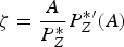 is the environmental-quality elasticity of the world price of Z and ζ > 0;
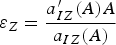 is the cleansing-good requirement elasticity of Z,
 are the shares of labour and of intermediate good respectively in the unit cost of producing good Z.
At the initial price of the intermediate good, requirement of higher environmental quality increases the cost of production. Competition ensures that the price of the intermediate good falls so that the exporters still earn zero profit. The fall in the price of the intermediate good is:

where 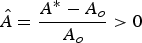 and
 denote the proportional change in the price of the intermediate good.
Referring back to figure 1, the C Z (A, P I) curve now comes down and cuts the P Z* (A) line from below at a point corresponding to the minimum standard A*. Note that, although the zero-profit condition is restored through a decline in the price of the intermediate good, it cannot restore the marginal condition (9) simply because the initial optimum environmental quality and price of the intermediate good were unique.
The change in environmental quality of exports affects the aggregate employment through changes in the level of production of the two traded goods and the productivity effects.

where 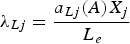 is the employment-share of sector j.
The direct impact of the productivity effect on unskilled labour (captured by the third term in equation (19)) is negative as the per-unit requirement (at initial output levels) in the traded sectors falls. However, there is also an indirect effect. The productivity effects change the output levels of the traded goods through changes in the factor prices, output of the intermediate good and the effective supply of skilled labour. The change in the intermediate sector is of prime importance. As a minimum standard is imposed, requirement of the intermediate good per unit of Z increases, increasing the demand for I. Since the supply of skilled labour is fixed, the supply of the intermediate good would not have increased to match the increase in demand had there been no change in the productivity of skilled labour. The productivity effect works through two channels in the intermediate sector. First, as the productivity of skilled labour increases, it increases the effective supply of skilled labour and allows an expansion of the intermediate sector by drawing some capital from the T sector. Hence there is an expansion of the intermediate sector and the dirty export sector but a contraction of the composite traded sector. As we have assumed that the dirty export sector is relatively more labour intensive, the employment generation in the Z sector compensates for the loss in the T sector. We call this the direct skilled-labour productivity effect. Second, the productivity effect affects the wage rate of skilled labour to return-to-capital ratio and induces a substitution between skilled labour and capital. While the return to capital declines due to competitive forces in the traditional export sector, the change in the wage rate of skilled labour is not as unambiguous, as it depends on several factors like the productivity effect in the three sectors, the environmental-quality elasticity of the world price of Z (ζ) and the cleansing-input requirement elasticity of Z (ɛZ).Footnote 9 If the ratio falls, then skilled labour is substituted for capital and some capital is released, allowing the composite traded sector to expand. However, as the supply of skilled labour is limited, even after an improvement in productivity, the shift towards a more skill-intensive technology will tend to reduce the output of I and hence that of Z. However, if the w S/r ratio rises, then the technology in the intermediate sector becomes more capital intensive, and there is withdrawal of capital from the T sector which contracts. The capital-intensive technology in I now allows a further increase in production of the intermediate good, causing expansion in the dirty export sector. Thus, how the employment will change due to the factor-substitution effect induced by the skilled-labour productivity effect depends on the direction of movement of the w S/r ratio, and, again, on the relative intensity rankings. The change in the output in the three sectors and the aggregate employment can then be written as:Footnote 10


where  , so that


where 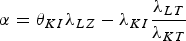 and

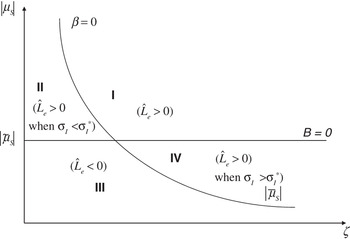
As explained before, the direct skilled productivity effect (captured by the last term in the parentheses in (23)) generates employment, while the direct unskilled-labour productivity effect (captured by the third term) results in an employment loss. As there is a trade-off between environmental quality and quantity of Z, any improvement A, other things remaining constant, will reduce the production of Z, and this will result in some loss in employment. This negative input-intensity effect is captured by the second term in the parentheses of (23). The first term in parentheses in (23) captures the factor substitution effect and, as explained later, the direction and extent of such changes depend on the factor substitution elasticity (σI) and the sign of α β. On the whole, the change in aggregate employment following a binding minimum environmental standard is ambiguous. However, the above discussion and the expressions for α and β show that the environmental-quality elasticity of the world price of Z (ζ), and the skilled-labour productivity change μS, are the two important parameters that determine the overall direction of change in aggregate employment. We derive necessary and sufficient conditions for an overall employment increase in terms of these two parameters in the analysis that follows. To facilitate our analysis, let

such that  .
Let  be the absolute value of μS such that B = 0 for any given set of values of the other parameters:

Thus for  (shown in figure 2 by the locus labelled
 or B = 0), the employment change equals
 . Similarly, we define
 as the absolute value of μS such that β = 0:

Since  is inversely related to ζ, the locus β = 0 is a negatively sloped curve in figure 2. These two loci, labelled
 (or B = 0),
 (or β = 0), divide the (ζ, |μS|) space into four regions that are labelled counterclockwise as regions I through IV.Footnote 11
Employment change when α > 0

Finally,

When α > 0, there is scope for increase in aggregate employment in regions I, II, and IV, while in region III employment will fall when environmental standards are imposed. However, when α < 0, then aggregate employment may increase in regions I, II and III, and decrease in region IV. Conditions for increase in aggregate employment of unskilled labour are given in the following table:

Where

An imposition of environmental standards will always result in an employment expansion when α > 0 in region I and α < 0 in region II, while there is no scope of employment generation when α > 0 in region III and α < 0 in region IV. In the rest of the cases employment increase depends on parametric restrictions on the factor substitution elasticity.
The need for restrictions on the value of σI is as follows. In region I, the combined impact of the productivity and the input-intensity effect on aggregate employment is positive (B > 0). As skilled wage rate to return-to-capital ratio rises and there is a substitution of capital for skilled labour in the intermediate sector, capital is withdrawn from the T sector, resulting in its contraction, and some employment loss. If the labour intensity of T is very small compared to Z (α > 0), then the employment loss is small and not powerful enough to bring down aggregate employment. However, if labour intensity of T is not that small (α < 0), then aggregate employment will rise only when σI is small (σI < σI*), and the rise in w S/r ratio causes a small substitution between skilled labour and capital. In this case capital withdrawn from T will be small, resulting in a small contraction in that sector and a small enough employment loss which can be offset by the employment increase due to the combined impact of the productivity and the input-intensity effect. The conditions in regions II through IV can be explained in a similar manner.
Given these observations we can summarize the conditions for overall employment increase in the following proposition:
Proposition 1
For all sets of values of (ζ, |μS|) such that  , aggregate employment rises when (i) αβ > 0, or (ii) αβ < 0 and σI < σI*. But for all sets of values of (ζ, |μS|) such that |μS| < ~μS, aggregate employment rises only when αβ > 0 and σI > σI*.
Proof Follows from figure 2 and the above discussion.
The above discussions also clearly bring out the importance of the productivity effect for an employment expansion. Had there been no productivity effect of an improvement in environmental quality, there would have been no scope for increase in aggregate employment for any α > 0. This is evident from the fact that for μZ = μT = μS = 0, the employment change denoted by  would equal

Thus, α < 0 is a necessary condition for an employment expansion in the absence of the productivity effects of an environmental-quality standard, which narrows down the scope for employment generation substantially. More precisely,
Proposition 2
If environmental-quality improvement has no effect on labour productivities, a binding minimum standard raises aggregate employment only when the labour intensity of unskilled labour in the traditional traded sector is low such that α < 0 and  , where
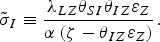
Proof Follows from (29). Thus, when there are no productivity effects, an environmental standard can generate employment with restrictions on the elasticity of substitution ( ) only if α < 0. The following lemma specifies further implications of the productivity effects along with the other assumptions:
Lemma 1
The critical values of the skilled-labour productivity change and the factor-substitution elasticity defined in (25), (26) and (28) have the following specific relationship with the parameters of the model:


Larger absolute values of μZ and μT mean that the productivity effect of an environmental standard is stronger and per-unit requirements of unskilled labour are smaller. Hence, from the above lemma it follows that a stronger productivity effect causes region I to shrink and region III to expand. Thus, when α > 0, the employment expansion will be unconditional for a smaller set of values of (ζ, |μS|). As region III expands, employment falls for a larger set of values of (ζ, |μS|), making the set of parameter values for which employment falls when α > 0 larger. However, as the critical value of the factor-substitution elasticity (σI*) falls as productivity effect in the Z-sector improves, the condition for an employment expansion in this region when α < 0 is now less stringent. This condition, on the other hand, gets more stringent when the productivity effect is stronger in the composite traded sector. Finally, a greater marginal willingness-to-pay of the foreign buyers for a better environmental-quality export (captured by the value of the elasticity ζ) expands regions I and II (where employment expansion does not depend on any other condition when α > 0 and α < 0 respectively) and also makes the factor-substitution elasticity condition for employment expansion (in regions III and IV) less stringent.
4. Discussion
In this section we discuss three issues. First, how the flexible coefficient in the traded sectors changes our employment result stated in Proposition 1. Second, what happens if we assume that T is relatively more labour intensive than Z, and third what happens if we assume that capital is directly employed in the production of the dirty good Z.
4.1. Flexible production coefficients
Suppose the production technology permits us to make alternative choices of a IZ, a LZ, a KT and a LT with the change in relative factor prices. So now the direction of change in aggregate employment will also be determined by the change in the production techniques in the traded good sectors. First of all, note that by (17) an improvement in the environmental quality lowers the price of the intermediate good. With (real) wage rigidity, this induces the producers of good Z to use less labour-intensive production techniques. Hence, the demand for labour on this account declines. On the other hand, producers of the composite traded good T use a relatively more labour intensive production technique since the rate of return to capital rises. On this account the demand for aggregate employment rises. The extent of the fall and rise in demand for unskilled labour depends on the factor-substitution elasticity in the Z and T sectors respectively. Therefore, there can be a net increase in the demand for and consequently employment of unskilled labour when the factor substitution elasticity in the T-sector is sufficiently high.
4.2. Importance of the factor-intensity assumption
Suppose that the composite traded good T is more labour intensive than the dirty export Z. That is, λLZλKT < λKIλLT. Referring back to equations (24) and (27), we see that now B < 0,α < 0. So regions I and II now disappear and regions III and IV, when α < 0, are now the only relevant cases. In region IV, when B < 0 and αβ < 0, employment will fall. However, if σI > σI*, then it is possible to generate employment in region III (i.e. when β < 0). Thus, even if we relax the intensity assumption made in equation (4), the employment-generating result remains intact qualitatively.
4.3. Dirty good produced with capital, unskilled labour and the cleansing good
If we consider a more general structure where the dirty good is produced with unskilled labour, capital and the intermediate (cleansing) good, the production structure of other goods remaining the same as in the original model, then equations (6) and (15) now become


The change in aggregate employment following imposition of environmental standards is

where 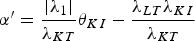 and
 .
Thus, the impact of environmental standards on aggregate employment remains the same qualitatively when capital is directly used in the production of the dirty good and conditions for employment generation can be derived in the same manner as before.
5. Conclusion
Popular argument in the South regarding environmental standards often projects a trade-off between aggregate employment of unskilled labour and such standards. While there may be other more valid grounds for objections to environmental standards and their uniformity, this paper demonstrates that the employment argument may be less appealing than is often projected. In fact, when the productivity effect of environmental regulation is taken into account, the case for standards is strengthened and under quite reasonable restrictions on the parameters, imposition of minimum environmental standards may raise aggregate employment of unskilled labour.
Appendix

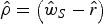 .



II. Output changes
From the full employment condition of skilled labour (14),

where
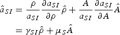
where 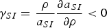 .
By similar logic, we can write:

where 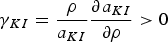 .
Now, note that the least-cost input choice condition is given by

Next, from the definition of factor substitution elasticity (12) we can write:

Hence, using (A.5) and (A.8), we can rewrite (A.4) as:

Now from the market clearing condition (13) for the non-traded intermediate good, we obtain:

Using (A.9) yields the change in the output of the dirty exports as:

On the other hand, from the full employment condition for capital we get

Proceeding as above, we can write âKI as

Substitution of (A.9) and (A.13) in (A.10) yields:

 , which is satisfied by the above set of assumptions.
 -locus may lie wholly above the point of intersection between the other two loci. However, except for categorization of different regions in terms of employment increase and decline, the essence of the argument remains the same.