


1. Introduction
Improvements in human longevity have been a global phenomenon, largely driven by sustained advances in living standards, medical care, and social protection systems. However, increasing longevity also poses significant financial challenges. Public pension systems, for instance, are under growing pressure as retirees spend longer periods in retirement, while expenditures on long-term care (LTC) are expected to increase substantially. Indeed, gains in life expectancy do not necessarily imply corresponding improvements in healthy life expectancy. As populations age, the prevalence of chronic conditions, functional limitations, and disability tends to increase, leading to a greater demand for LTC services and support.
Life annuities represent a highly effective mechanism for addressing individual longevity risk during retirement by ensuring deterministic lifelong income streams to policyholders. However, the annuity market remains notably under-penetrated, as retirees tend to annuitize their wealth at levels significantly below theoretical expectations (Brown, Reference Brown2007). There are many possible explanations for this phenomenon: from the policyholder’s perspective, annuity contracts exhibit significant inflexibility and lack sufficient liquidity to accommodate consumption adjustments in response to unforeseen financial shocks. This rigidity arises from the predetermined nature of periodic payouts and the irrevocable nature of the purchase decision (Chai et al., Reference Chai, Horneff, Maurer and Mitchell2011). Additionally, conventional annuities do not offer a bequest feature, potentially conflicting with policyholders’ preferences to leave inheritances (Inkmann et al., Reference Inkmann, Lopes and Michaelides2011). The presence of public pension systems further diminishes retirees’ demand for annuities. Furthermore, insurers impose higher premiums to counteract adverse selection, a practice often perceived by policyholders as inequitable pricing (Friedman & Warshawsky, Reference Friedman and Warshawsky1990).
Regarding the LTC needs, the LTC insurance products may be perceived by individuals (at least theoretically) as a relevant vehicle to transfer their individual disability risk. Traditional LTC insurance products have historically been marketed separately from annuity products. However, their take-up rates remain relatively low both across OECD countries (see, e.g., OECD, 2011) and worldwide (Braun et al., Reference Braun, Kopecky and Koreshkova2019). The limited demand for LTC insurance has been attributed to several factors, including substantial premium loadings, informational asymmetries, and consumers’ limited understanding of LTC-related risks and insurance products, as discussed by Brown and Finkelstein (Reference Brown and Finkelstein2007). In addition, adverse selection increases insurers’ operating expenses through higher underwriting, distribution, and claims management costs (Cornell et al., Reference Cornell, Grabowski, Cohen, Shi and Stevenson2016). Taken together, these limitations have constrained the development of the LTC insurance market, and at the same time, have stimulated the development of hybrid retirement-income and LTC products, combining longevity protection with coverage against LTC needs. For instance, Getzen (Reference Getzen1988) introduced the concept of longlife insurance, a product that integrates deferred annuity benefits with health insurance and LTC coverage. This approach is designed to simultaneously mitigate the risks of chronic illness and longevity, thereby addressing adverse selection issues that affect both LTC insurance and annuities. Haberman and Pitacco (Reference Haberman and Pitacco1999) and Leung (Reference Leung2006) combine LTC insurance with whole life insurance, an approach that has been explored more recently by Chen et al. (Reference Chen, Fuino, Sehner and Wagner2022), where the analysis incorporates both the insurer’s financial perspective and the policyholder’s willingness to pay for the LTC option. Murtaugh et al. (Reference Murtaugh, Spillman and Warshawsky2001) proposed the life care annuity (LCA), a hybrid product that combines life annuity benefits with LTC insurance. An expanding body of theoretical and empirical literature highlights the benefits and potential extensions of LCAs. Key contributions include, among others, studies by Webb (Reference Webb2009), Gong & Webb (Reference Gong and Webb2010), Levantesi & Menzietti (Reference Levantesi and Menzietti2012), Brown & Warshawsky (Reference Brown and Warshawsky2013), Shao et al. (Reference Shao, Sherris and Fong2017), Hsieh et al. (Reference Hsieh, Wang, Chiu and Chen2018), Ventura-Marco et al., Reference Ventura-Marco, Vidal-Meliá and González2023.
In particular, Hsieh et al. (Reference Hsieh, Wang, Chiu and Chen2018) proposed a variable life care annuity with Guaranteed Lifetime Withdrawal Benefits (LCA-GLWB) that extends the traditional GLWB variable annuity by providing LTC payouts when policyholders experience predefined frailty states (e.g., impairments in activities of daily living (ADLs), see Pritchard (Reference Pritchard2006)). Under the general structure of a GLWB variable annuity contract, the policyholder is allowed to withdraw a given fraction of the benefit base each year as long as she remains alive, even if the policy account is depleted, and any remaining account value at death is paid to the beneficiary as a death benefit. Such an LCA-GLWB product integrates two notable benefits. It offers a cost-effective solution for policyholders compared to purchasing standalone products, such as LTC insurance and variable annuity with GLWB. For insurers, it provides a mechanism to mitigate adverse selection risks. A recent generalization of Hsieh et al. (Reference Hsieh, Wang, Chiu and Chen2018) proposal was presented by Apicella et al. (Reference Apicella, Gaudenzi and Molent2025), where the authors price the contract using a tree-based method (similar to Appolloni et al. (Reference Appolloni, Caramellino and Zanette2015)), by considering a dynamic withdrawal strategy (as e.g., in Forsyth and Vetzal (Reference Forsyth and Vetzal2014), Bacinello et al. (Reference Bacinello, Maggistro and Zoccolan2024)) and referring to the Cox-Ingersoll-Ross process for modeling the stochastic interest rate (Cox et al., Reference Cox, Ingersoll and Ross1985). The proposed product, denoted as GLWB-LTC, beyond ensuring the policyholders the right to make guaranteed withdrawals, provides an annual disability allowance if their health state corresponds to a disability condition covered by the contract. Numerical simulations indicate that the dynamic withdrawal strategy enhances the appeal of the GLWB-LTC product by offering policyholders greater flexibility in managing their savings for financing disability-related expenses.
Another recent study combining GLWB with an LTC option was conducted by Yang et al. (Reference Yang, Chen, Cui and Zhang2024). In their analysis, the insurer adjusts guaranteed withdrawal rates based on the health status of policyholders, which is modeled as a continuous-time, finite-state Markov process. The valuation of the GLWB annuity with the LTC option is framed as a discrete stochastic control problem and a backward recursion methodology is employed, as in Bacinello et al. (Reference Bacinello, Maggistro and Zoccolan2024), for the analysis of dynamic withdrawal strategies. The study also includes a sensitivity analysis examining the LTC option’s impact on contract value.
Against this background, this manuscript proposes a pricing framework for a variable annuity with a deferred GLWB rider and an LTC option. The contract consists of two distinct phases: an accumulation phase followed by an income phase. During the former, the policyholder pays an initial lump-sum premium and may subsequently) make additional premium contributions (fund purchases). These contributions, together with the roll-up feature, increase both the policy account value and the benefit base. While GLWB rider-related withdrawals are not available during the accumulation period, the contract provides LTC protection by granting access to guaranteed withdrawals upon the onset of LTC disability. At the end of the accumulation period, the contract enters the income phase, during which the GLWB rider becomes effective and provides guaranteed lifetime withdrawals. The LTC coverage remains in force throughout this phase, so that the guaranteed withdrawal benefit is contingent on the policyholder’s health status. Specifically, LTC-disabled policyholders are entitled to enhanced withdrawal rates relative to healthy policyholders. The contract also provides that the policyholder retains the right to fully surrender the contract during both the accumulation and the income phases.
Compared with the existing literature, the main contributions of our work are twofold. First, we extend the GLWB framework considered in Bacinello et al. (Reference Bacinello, Maggistro and Zoccolan2024) and Yang et al. (Reference Yang, Chen, Cui and Zhang2024), among others, by introducing a deferred GLWB rider preceded by an accumulation phase. In contrast, these studies consider variable annuities in which the GLWB rider becomes effective immediately after policy issuance, thus excluding any accumulation period. However, the accumulation period enables the benefit base to grow through additional fund purchases and roll-up features, potentially increasing future guaranteed withdrawals. This mechanism may reduce the attractiveness of early surrender, as policyholders forgo the opportunity to further enhance their future income guarantee. Moreover, the GLWB contract considered in Bacinello et al. (Reference Bacinello, Maggistro and Zoccolan2024) does not incorporate LTC coverage and therefore neglects the impact of LTC risk on the valuation of the contract and on policyholder behavior. The second contribution concerns the valuation methodology. We determine the risk-neutral contract value by formulating and solving a stochastic optimal control problem through dynamic programming, thereby accounting for the policyholder’s dynamic withdrawal strategy. To this end, we build upon the dynamic programming framework developed in Bacinello et al. (Reference Bacinello, Maggistro and Zoccolan2024), extending it to accommodate the features of the variable annuity contract we consider. More specifically, the introduction of both the accumulation phase and the LTC coverage enlarges the set of admissible policyholder actions. Indeed, the policyholder may make additional premium contributions during the accumulation period, and withdrawal decisions throughout the contract depend on the policyholder’s health status. Consequently, the verification of the bang-bang principle requires a two-stage backward induction procedure: the value function obtained for the income phase acts as the terminal condition for the backward induction associated with the accumulation phase. We prove that the set of optimal withdrawal strategies is finite and can be characterized by a limited number of discrete decisions, arising already during the accumulation phase. This result is particularly significant because, in the insurance literature, the existence of optimal bang-bang controls is usually assumed or established under strong structural assumptions, such as global convexity and monotonicity of the contract value function (see, e.g., Azimzadeh & Forsyth, Reference Azimzadeh and Forsyth2015; Huang & Kwok, Reference Huang and Kwok2016) and, in some cases, suitable scaling properties (see, e.g., Huang et al., Reference Huang, Zeng and Kwok2017). In our setting, however, the set of admissible withdrawal strategies is richer, as it includes additional premium contributions, health-state-dependent decisions, and LTC-contingent withdrawals, yet the optimal strategy can still be characterized by a finite set of bang-bang controls.
We test the proposed theoretical framework through numerical examples by assuming that the underlying asset price follows an exponential Lévy process. The transition and mortality probabilities are taken from Baione et al. (Reference Baione, Conforti, Levantesi, Menzietti and Tripodi2016), where they are calibrated using mortality data provided by the Italian National Social Security Institute (INPS). We first assess the numerical accuracy of the proposed dynamic programming algorithm. Then, we perform a sensitivity analysis of the initial contract value, with and without the LTC option, with respect to the contract parameters and the interest rate, distinguishing between male and female policyholders. Afterwards, we investigate the optimal withdrawal strategies at different points in time, highlighting how they vary across health states, genders, and contract parameters. Furthermore, we assess the robustness of both the initial contract value and the optimal withdrawal strategies under alternative specifications of the asset dynamics. The numerical analysis concludes by inspecting the sensitivity of the fair rider fee to changes in the contractual and demographic assumptions.
The paper is structured as follows. Section 2 outlines the structure of the variable annuity contract. Section 3 presents our valuation problem, defining the contract value as an optimal withdrawal problem and introducing the dynamic programming equations used to solve it. Furthermore, the validity of the bang-bang condition is established, and the evaluation algorithm is described in detail. In Section 4, we first present an accuracy analysis of our dynamic programming algorithm. We then present a sensitivity analysis of the contract value, optimal withdrawal strategies and fair fees with respect to both contract parameters and gender. The robustness of the initial contract value and the optimal withdrawal strategies are also investigated under alternative specifications of the underlying asset dynamics. Section 5 concludes.
2. The contract design
In this section, we describe the GLWB rider in our variable annuity contract that includes an accumulation phase and an LTC option. This rider provides the policyholder not only with the right to make periodic withdrawals from her personal account throughout her life, but also with LTC benefits if she becomes disabled.
At the contract inception, the
 $x$
-aged policyholder pays an upfront single premium
 $P$
, which is entirely invested in a well-diversified and non-dividend paying mutual fund of her choice. We denote by
 $S_t$
the market price at time
 $t$
of each unit of this fund, which drives the return on the investment portfolio built up from the policyholder’s initial payment. We denote by
 $W_t$
the value of this portfolio (personal or policy account) at time
 $t$
. In particular, at
 $t=0$
, an accumulation phase begins and lasts until a fixed contractual time
 $t=T$
, predetermined in the contract. During this phase, the policyholder can place additional purchases of funds, up to a constant fraction
 $0\lt \pi \lt 1$
of the benefit base, denoted by
 $A_t$
, beyond the initial premium. Such purchases would increase both the benefit base and policy account value. Moreover, if the policyholder becomes disabled during this phase, the LTC option is activated, allowing guaranteed withdrawals at a fixed rate from her personal account on specified dates to cover healthcare costs. Subsequently, for
 $t\gt T$
, the income phase begins and the policyholder exercises the GLWB guarantee, enabling her to make periodical withdrawals of different amounts from her personal account at specified dates for the whole life, even if the account value is reduced to zero.
The cost of the GLWB rider with the LTC option is funded via periodic charges applied proportionally to the policy account value (insurance fees). The guaranteed withdrawal amount is determined, both in the accumulation and income phase, as a fixed percentage (withdrawal rate) of the benefit base which is initially set equal to the single premium and is adjusted upward via the roll-up (or bonus) feature that applies when no withdrawal is made on a specified withdrawal date. Complete surrender of the policy, allowed in both the accumulation and income phase, refers to the withdrawal of the whole personal account if it exceeds the guaranteed amount. As a result, the variable annuity contract terminates. Another event triggering the contract’s termination is the policyholder’s death. In this case, the remaining policy account value is paid to the beneficiary as a death benefit.
From now on, we assume that: (i) withdrawals are allowed on a predetermined set of equidistant dates and, without loss of generality, we take the distance between two consecutive withdrawal dates as unit of measurement of time; (ii) the death benefit is paid to the beneficiary on the withdrawal date immediately following the policyholder’s death.
We now formalize what was just described. Let
 $\tau$
denote the time of death of the policyholder, so that withdrawals are allowed only at times
 $j=1,2,\dots$
provided that
 $\tau \gt j$
. Moreover, let
 $\lambda$
be the time of permanent disability with the convention that if
 $\lambda \geq \tau$
the policyholder never becomes disabled. We also introduce the variable
 \begin{equation*} z_j=\mathbf{1}_{\{\lambda \gt j\}}=\begin{cases} 1 & \text{if} \quad \lambda \gt j\\ 0 & \text{if} \quad \lambda \leq \, j \end{cases}\!, \end{equation*}
which defines the healthy status of the policyholder at time
 $j$
. In particular, if
 $z_j=1$
the policyholder is healthy, otherwise she is disabled and will remain so indefinitely. The assumption of permanent disability is in line with some studies (see e.g., Ferri & Olivieri, Reference Ferri and Olivieri2000 and Hanewald et al., Reference Hanewald, Li and Shao2019) which do not incorporate recovery – defined as the transition from a disabled state to a healthy state – on the grounds that LTC impairments are generally chronic and that the probability of recovery is negligible. According to the policyholder’s health status at time
 $j=1, \ldots , T, T+1, \ldots$
, we consider a different withdrawal rate: we denote by
 $g_j^{(i)}=g^{(i)}$
the withdrawal rate of the policyholder which is disabled
 $(i)$
at time
 $j$
, while let
 \begin{equation} g_j^{(h)}=\begin{cases} 0 & \text{if} \quad j\leq T\\ g^{(h)}& \text{if} \quad j\gt T \end{cases}, \end{equation}
be the withdrawal rate of the healthy
 $(h)$
policyholder, with
 $g^{(i)}\neq g^{(h)}$
. The guaranteed amount that can be withdrawn at time
 $j=1, \cdots , T$
is equal to
 $g^{(i)}A_j$
, while for
 $j=T+1, \ldots$
, it is equal to
 $g^{(m)}A_j$
,
 $m=h, i$
, and the return on the reference fund over the interval
 $[\, j-1, j]$
is
 \begin{equation} R_j=\frac {S_j}{S_{j-1}}-1,\quad j=1,2,\dots \;. \end{equation}
We stress that the policyholder is not obliged to withdraw the guaranteed amount: she can withdraw less than such amount, or even more if not exceeding the policy account value. We denote by
 $y_j$
the actual withdrawal made by the policyholder at time
 $j$
. This withdrawal strategy is admissible if it belongs to the set of admissible withdrawal strategies
 $Y=(Y_j)_{j\in \mathbb{N}^+}$
where
 \begin{equation} Y_j=Y_j^{(h)}\mathbf{1}_{\{\lambda \gt j\}}+Y_j^{(i)}\mathbf{1}_{\{\lambda \leq \, j\}}, \end{equation}
and
 \begin{equation} Y_j^{(m)}=\begin{cases} [\!-\pi A_j, W_j], \quad & m=h;\ j=1, \ldots , T \\ [\!-\pi A_j, \max \{g^{(i)}A_j, W_j\}], \quad & m=i;\ j=1, \ldots , T\\ [0, \max \{g^{(m)}A_j, W_j\}], \quad & m=h,i; \ j=T+1, \ldots \end{cases}\!. \end{equation}
If the policyholder does not withdraw at time
 $j$
, the benefit base is proportionally increased according to the roll-up rate denoted by
 $b_j^{(m)} \in (0,1)$
,
 $m=h,i$
, and according to any possible additional purchase allowed in the accumulation phase only. If, instead, the withdrawal exceeds
 $g^{(m)}A_j$
, it is proportionally reduced according to the so called ‘pro-rata’ adjustment rule. Then, to describe the evolution of the benefit base, we introduce the following function
 \begin{equation} a_{j+1}^{(m)}(W_j, A_j, y_j)=\begin{cases} A_j\big (1+b_j^{(m)}\big )-y_j & \text{if} \quad y_j\leq 0,\\[3pt] A_j & \text{if} \quad 0\lt y_j\leq g^{(m)}A_j,\\[3pt] \displaystyle A_j\frac {W_j-y_j}{W_j-g_j^{(m)}A_j} & \text{if} \quad g_j^{(m)}A_j\lt y_j\leq W_j \end{cases} \!, \quad m=h,i, \ j=1,2,\dots \end{equation}
from which we get the evolution of the benefit base:
 \begin{equation} A_{j+1}=a_{j+1}^{(h)}(y_j, W_j, A_j)\mathbf{1}_{\{\lambda \gt j\}}+a_{j+1}^{(i)}(y_j, W_j, A_j)\mathbf{1}_{\{\lambda \leq \, j\}}, \end{equation}
with
 $A_1=A_0=P$
.Footnote
1
Conversely, if withdrawals exceed the guaranteed amount, a proportional penalization on the surplus appliesFootnote
2
according to a penalty rate, denoted by
 $k_j^{(m)} \in [0,1)$
,
 $ m=h,i$
. Therefore, the net amount (cash-flow) received by the policyholder at time
 $j$
is given by
 \begin{equation} C_j^{(m)}(y_j, A_j)= y_j-k_j^{(m)}\max \{y_j-g_j^{(m)}A_j, 0\},\quad m=h, i;\ j=1,2,\dots \,;\ y_j\in Y_j. \end{equation}
The policy account value evolves according to the following equation:
 \begin{equation} W_{j+1}=w(W_j, R_{j+1}, y_j)=\max \{W_j-y_j,0\}(1+R_{j+1})(1-\varphi ), \quad j=0,1,\dots , \end{equation}
where
 $\varphi \in (0,1)$
is the insurance fee rate,
 $W_{0}=P$
and
 $y_{0}=0$
. Note that
 $0$
is an absorbing barrier for
 $W$
because, once it becomes null, it remains so forever. The contract, however, continues while
 $A_t\gt 0$
(and the insured is still alive). Finally, in case of death in the time interval
 $(j-1, j]$
, the death benefit, paid at time
 $j$
, is
 \begin{equation} B_j=W_j,\quad j-1\lt \tau \leq \, j\;,\quad j=1,2,\dots \;. \end{equation}
We notice that in case of surrender at time
 $j$
, the contract is automatically closed because Equations (6) and (8) imply
 $A_t=W_t=0$
for all
 $t\gt j$
, hence no further withdrawals are admitted, nor a death benefit will be paid.
3. The valuation problem
We assume a frictionless market in which all agents are price-takers, assets are perfectly divisible, and no taxes or transaction costs exist. Furthermore, we assume that markets are arbitrage-free, thus ensuring the existence of equivalent risk-neutral measures. Given the incompleteness of insurance markets, especially when pricing is conducted at the single-contract level rather than at portfolio one, infinitely many risk-neutral measures exist, and we suppose that the insurer selects one among them, according to its own preferences, for pricing purposes. We assume independence between biometric and financial risks, as well as deterministic transition and death probabilities. Therefore, we account only for the idiosyncratic component of biometric risk, ignoring systematic deviations between expected and realized mortality. Considering the above, let us consider a complete probability space
 $(\Omega , {\mathcal F}, Q)$
, equipped with a complete and right continuous filtration
 $\mathbb{F} =\left (\mathcal{F}_t\right )_{t\geq 0}$
, where
 $Q$
is the risk-neutral probability measure selected by the insurer. In addressing financial risk, we assume a constant and deterministic instantaneous interest rate, denoted by
 $r$
, for our valuation algorithm. Nonetheless, the theoretical results developed in the following remain valid under a more general framework in which the interest rate evolves according to a Markovian stochastic process
 $(r_t)_{t\geq 0}.$
See Section 1 of the Supplementary Material for further details, where an analysis of variations in contract value and withdrawal strategies is also provided, using the term structure of U.S. risk-free interest rates as a benchmark against the constant rate adopted in the manuscript.
We model the reference portfolio value
 $S_t$
as an exponential Lévy process:
 \begin{equation} S_t=S_0 \text{e}^{(r+d)t+X_t}, \end{equation}
where
 $(X_t)_{t\geq 0}$
, with
 $X_0=0$
, is a
 $\left (\mathbb{F},Q\right )$
-Lévy process, and
 $d$
represents an adjustment so that
 $S_t\,\text{e}^{-rt}$
is a
 $\left (\mathbb{F},Q\right )$
-martingale. Thus,
 $X_t$
is right-continuous with left limits paths,
 $X_s-X_t$
is independent of
 $(X_u)_{0\leq u\leq t}$
and is distributed as
 $X_{s-t}$
, for
 $0\leq t\lt s$
. Furthermore,
 $X_t$
is completely determined by its characteristic function
 \begin{equation} \Phi _t(u)\,:\!=\,\mathbb{E}^Q\left [\text{e}^{i u X_t}\right ]=[\Phi _1(u)]^t, \end{equation}
where
 $i$
is the unit imaginary number. Then, the drift adjustment
 $d$
is given by
 \begin{equation} d=-\frac {1}{t}\ln \Phi _t(\!-i)=-\ln \Phi _1(\!-i). \end{equation}
All moments of
 $X_t$
can be numerically recovered from the knowledge of
 $\Phi _t$
(when not available in closed form), and if
 $\Phi _t$
is integrable, then
 $X_t$
has density given by:
 \begin{equation} f_t(\phi )=\frac {1}{2\pi }\int ^{\infty }_{-\infty }\text{e}^{-iz\phi }\Phi _t(z)\text{d}z. \end{equation}
The transition and death probabilities are given as follows. Let
 \begin{equation*} \begin{aligned} & p_{j}^{h,h}=Q(\tau \gt j+1,\, z_{j+1}=1\, |\, z_j=1, \tau \gt j), \\ & p_{j}^{h,i}=Q(\tau \gt j+1,\, z_{j+1}=0\, |\, z_j=1, \tau \gt j), \end{aligned} \qquad j=0, 1, \ldots , \end{equation*}
be the one-year transition probabilities which represent, respectively, the probability to be alive and healthy at age
 $x+j+1$
, and to be alive but disabled at age
 $x+j+1$
, both conditional on survival and to being healthy at age
 $x+j$
. Moreover, let
 \begin{equation*} p_{j}^{i,i}= Q(\tau \gt j+1,\, z_{j+1}=0\, |\, z_j=0, \tau \gt j), \qquad j=1, 2, \ldots , \end{equation*}
be the probability to be alive and disabled at age
 $x+j+1$
conditional on survival and to being disabled at age
 $x+j$
. Note that
 $p_{j}^{i,h}=0$
for the hypothesis of permanent disability.
Concerning the death probabilities, let
 \begin{equation*} \begin{aligned} &q_{j}^{h}=Q(\tau \leq \, j+1\, |\,\tau \gt j, z_j=1), \qquad j=0, 1, \ldots ,\\ &q_{j}^{i}=Q(\tau \leq \, j+1\, |\,\tau \gt j, z_j=0), \qquad j=1, 2, \ldots , \end{aligned} \end{equation*}
be the probabilities of dying before age
 $x+j+1$
conditional on survival and to being healthy or disabled, respectively, at age
 $x+j$
. Note that both
 $p_{j}^{i,i}$
and
 $q_{j}^{i}$
takes value for
 $j=1, 2, \ldots ,$
because in our model at contract inception (
 $j=0$
) the policyholder has to be healthy, i.e.,
 $z_0=1$
.
We now define the initial value of the GLWB variable annuity with the LTC option. Since, as previously discussed, markets are incomplete and arbitrage-free, this value is not uniquely determined by replicating strategy. Moreover, in addition to uncertainty arising from biometric and financial risk factors, the cash flows generated by the contract – and hence their value – crucially depend on the policyholder’s behavior, which the insurer would ideally predict accurately. However, this is a challenging task. The uncertainty about the policyholder’s preferences (e.g., her specific utility function or subjective risk-neutral measure) is further amplified by information asymmetry, particularly concerning her health status. To address this issue, we assume that the insurance company fixes the risk-neutral measure
 $Q$
, intended to approximate the policyholder’s valuation preferences, and computes the initial contract value by maximizing the expected present value of all future cash flows generated by the variable annuity. We remark that the withdrawal strategy solving this maximization problem does not necessarily reflect the policyholder’s optimal preferences, but rather corresponds to the insurer-adverse withdrawal strategy, namely the strategy that maximizes the value of the contract liabilities under the assumed model. To formally translate our problem, we consider the admissible withdrawal strategy in (3)–(4) and define the initial value of the GLWB variable annuity with the LTC option as the solution of the following optimization problem:
 \begin{equation} \begin{aligned} V_{0}=\sup _{y \in Y} \mathbb{E}^Q\Bigg [\sum _{j=1}^n \text{e}^{-rj}&\left (\mathbf{1}_{\{\tau \wedge \lambda \gt j\}}\,C_j^{(h)}(y_j,A_j)+ \mathbf{1}_{\{\lambda \leq \, j\lt \tau \}}\,C_j^{(i)}(y_j,A_j) +\mathbf{1}_{\{j-1\lt \tau \leq \, j\}}W_j\right )\\ &+\text{e}^{-r(n+1)}\mathbf{1}_{\{\tau \gt n\}}W_{n+1}\Bigg ], \end{aligned} \end{equation}
where
 $C_j^{(m)} \, (m=h,i)$
and
 $W_j$
satisfy Equation (7) and (8), respectively. Here,
 $n=\omega -x$
, with
 $\omega$
denoting the maximum attainable ageFootnote
3
for the policyholder, beyond which her survival probability is zero. The contract value
 $V_0$
depends on the single premium
 $P$
through the initial level of the benefit base and the policy account, but does not necessarily coincide with it. When
 $V_0$
equals
 $P$
, we say that the contract is fairly priced, consistently with the actuarial equivalence principle. Referring back to the earlier comment about the insurer-adverse withdrawal strategy, when
 $V_0= P$
, the insurer is on the safe side, since the premium covers the expected present value of the benefits. To achieve a contract value exactly equal to
 $P$
, an appropriate choice of contract parameters is required. The key parameter usually chosen to get fair pricing, once all the other parameters are fixed, is the insurance fee rate
 $\varphi$
. Thus, the particular value of
 $\varphi$
which makes
 $V_0(P, P,1)=P$
will be referred to as fair fee rate.
3.1. Dynamic programming approach
In order to solve (14), we implement a dynamic programming algorithm for discrete stochastic control problems (see, e.g., Bertsekas, Reference Bertsekas2005 and Seierstad, Reference Seierstad2009). For each
 $j=0,1,\ldots , n+1,$
and each value of policy account
 $W_j$
, benefit base
 $A_j$
and health status
 $z_j$
, we denote by
 $V_j(W_j, A_j, z_j)$
the contract value at time
 $j$
(before the periodic withdrawal) and by
 $v_j(W_j, A_j, z_j)$
the contract value at the same time if the policyholder is alive. Clearly
 $V_j(W_j, A_j, z_j)=\mathbf{1}_{\{\tau \gt j\}}v_j(W_j, A_j, z_j)$
and
 $V_{0}=V_0(P,P,1)=v_0(P,P,1)$
. Since the algorithm proceeds backward, we take
 $n+1$
as the starting point and define the following terminal condition:
 \begin{equation} v_{n+1}(W_{n+1},A_{n+1},z_{n+1})\equiv 0. \end{equation}
Note that the specific value of
 $v_{n+1}$
is irrelevant since it is multiplied by the survival indicator
 $\mathbf{1}_{\{\tau \gt n+1\}}$
, which is almost surely zero, to determine the contract value
 $V_{n+1}$
.
Then, to proceed backward, we define the Bellman recursive equation of the problem as follows:
 \begin{align} &v_j(W_j, A_j, z_j)=\sup _{y_j \in Y_j}\Big ( \mathbf{1}_{\{\lambda \gt j\}}\ C_j^{(h)}(y_j, A_j)\,+\, \mathbf{1}_{\{\lambda \leq \, j\}}\ C_j^{(i)}(y_j, A_j) \\&\quad +\mathbb{E}^Q\big [\mathbf{1}_{\{\tau \leq \, j+1\}}w(W_j,R_{j+1},y_j)\text{e}^{-r}|W_j,A_j,z_j,\tau \gt j\big ] \\&\, \,\,\,\,\,+\,\mathbb{E}^Q\big [ \mathbf{1}_{\{\tau \gt j+1\}}v_{j+1}\big(w(W_j,R_{j+1},y_j),a_{j+1}^{(h)}(W_j,A_j,y_j)\,\mathbf{1}_{\{\lambda \gt j\}}+a_{j+1}^{(i)}(W_j,A_j,y_j)\,\mathbf{1}_{\{\lambda \leq \, j\}}, z_{j+1}\big)\text{e}^{-r}\nonumber\\ &\qquad \qquad |W_j,A_j,z_j,\tau \gt j\big ]\Big ),\qquad j=n,n-1,\dots ,1. \end{align}
In the first expectation of (16), using the stochastic independence between financial and demographic factors, the definition of the policy account value in (8), and the martingale property
 $\mathbb{E}^Q[(1+R_{j+1})e^{-r}]=1$
, we obtain
 \begin{equation} \mathbb{E}^Q\big [\mathbf{1}_{\{\tau \leq \, j+1\}}w(W_j,R_{j+1},y_j)\text{e}^{-r}|W_j,A_j,z_j,\tau \gt j\big ]=\max \{W_j - y_j,\,0\}(1-\varphi )Q(\tau \leq \, j+1\, |\, z_j, \tau \gt j). \end{equation}
In the second expectation, we can factorize the conditional
 $Q$
-expectation inside, and after applying the tower property, we obtain
 \begin{equation} \begin{aligned} &\mathbb{E}^Q\big [ \mathbf{1}_{\{\tau \gt j+1\}}v_{j+1}\big(w(W_j,R_{j+1},y_j),a_{j+1}^{(h)}(W_j,A_j,y_j)\,\mathbf{1}_{\{\lambda \gt j\}}+a_{j+1}^{(i)}(W_j,A_j,y_j)\,\mathbf{1}_{\{\lambda \leq \, j\}}, z_{j+1}\big )\text{e}^{-r}\\[5pt] &\qquad \qquad |W_j,A_j,z_j,\tau \gt j\big ]\\[5pt] &= \mathbb{E}^Q\big[v_{j+1}\big(w(W_j,R_{j+1},y_j),a_{j+1}^{(h)}(W_j,A_j,y_j)\,\mathbf{1}_{\{\lambda \gt j\}}+a_{j+1}^{(i)}(W_j,A_j,y_j)\,\mathbf{1}_{\{\lambda \leq \, j\}}, 1\big)\text{e}^{-r}\\[5pt] &\qquad \qquad |W_j,A_j,z_j\big]\,Q(\tau \gt j+1,\, z_{j+1}=1\, |\, z_j, \tau \gt j)\\[5pt] &+ \mathbb{E}^Q\big [v_{j+1}\big(w(W_j,R_{j+1},y_j),a_{j+1}^{(h)}(W_j,A_j,y_j)\,\mathbf{1}_{\{\lambda \gt j\}}+a_{j+1}^{(i)}(W_j,A_j,y_j)\,\mathbf{1}_{\{\lambda \leq \, j\}}, 0\big)\text{e}^{-r}\\[5pt] &\qquad \qquad |W_j,A_j,z_j\big ]\,Q(\tau \gt j+1,\, z_{j+1}=0\, |\, z_j, \tau \gt j). \end{aligned} \end{equation}
Finally, the initial contract value is:
 \begin{equation} \begin{aligned} v_0(P,P,1)=q^{h}_{0}P(1-\varphi )&+\mathbb{E}^Q\big [v_1(P(1+R_1)(1-\varphi ),P,1)\,e^{-r}\big ]p_0^{h,h} \\&+\mathbb{E}^Q\big [v_1(P(1+R_1)(1-\varphi ),P,0)\,e^{-r}\big ]p_0^{h,i}, \end{aligned} \end{equation}
where
 $q^{h}_{0}$
,
 $p_0^{h,h}$
and
 $p_0^{h,i}$
are defined as in Section 3.
3.2. Bang-bang analysis
The recursive equation (16) requires, at each time step
 $j=n,n-1,\dots 1$
, to solve a real-valued optimization problem where the domain
 $Y_j^{(m)}$
(4) of the single policy
 $y_j$
depends both on the health status of the policyholder and the contract phase (accumulation or income phase). Even if withdrawals can take place only once a year, for, e.g., a 50-year-old policyholder this would imply around 65 time steps. Moreover, at each time step the problem must be solved for every possible triplet of state variables
 $(W_j,A_j,z_j)$
and therefore the computational effort could be substantial. A property that would drastically reduce this effort is the bang-bang condition, which states that the set of the optimal withdrawals consists of a finite number of choices. In what follows, we prove this condition without assuming convexity or monotonicity of the contract value function. In particular, in the accumulation phase if the policyholder is healthy, the set of optimal withdrawals consists of three choices only: maximum allowable purchase, zero withdrawal, complete surrender, i.e., the maximization can be restricted to the subset
 $\{-\pi A_j, 0,W_j\}$
of
 $Y_j^{(h)}$
. If instead she is disabled, the set of optimal withdrawals consists of four choices only: maximum allowable purchase, zero withdrawal, withdrawal at the contractual amount, complete surrender, namely the subset
 $\{-\pi A_j, 0, g^{(i)} A_j, W_j\}$
of
 $Y_j^{(i)}$
. In the income phase, the set of optimal withdrawals again consists of three choices only: zero withdrawal, withdrawal at the contractual amount, complete surrender, and hence the maximization can be restricted to the subset
 $\{ 0, g^{(m)} A_j, W_j\}$
,
 $m=h, i$
.
The economic intuition behind this condition can be explained as follows according to the contract structure. In the accumulation phase, for the healthy policyholder could be convenient to purchase
 $y_j=-\pi A_j$
to maximize the benefit base (and thus future guaranteed withdrawals during the income phase), especially if her expected residual lifetime is sufficiently long. However, it is not advantageous to purchase an amount
 $y_j$
with
 $-\pi A_j\lt y_j\lt 0$
since the benefit base increase is not maximized. Also, the policyholder loses the advantage of investing her money outside the policy, potentially in a risk-free asset yielding more than the policy account (due to the insurance fee). Hence, the optimal strategy would be no-withdrawal (
 $y_j=0$
). It is possible to withdraw an amount
 $y_i\gt 0$
but it is subject to the withdrawal penalty
 $k_j y_j$
(see footnote 2) as well as to a second penalization due to the reduction of the benefit base according to the pro-rata rule, since the policyholder loses the roll-up incentive. This suggests that withdrawing the entire account value
 $W_j$
, i.e., surrendering the contract, may be more convenient.
For the disabled policyholder in the accumulation phase, the same arguments apply to
 $y_j=-\pi A_j$
and
 $y_j=0$
. If
 $0\lt y_j\lt g^{(i)}A_j$
, the policyholder loses the roll-up incentive without taking full advantage of the guarantee: if she does not need the entire amount
 $g^{(i)}A_j$
and prefers to benefit from the investment of what exceeds her needs, it may be preferable to invest this money in a risk-free asset, which, as just observed, yields more than the policy account value. On the other hand, if
 $W_j\gt g^{(i)}A_j$
, it is possible to withdraw an amount
 $y_j\gt g^{(i)}A_j$
, but in this case the withdrawal penalty
 $k_j(y_j-g^{(i)}A_j)$
is applied. Moreover, if
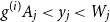 $g^{(i)}A_j\lt y_j\lt W_j$
, there is a second penalization due to the pro-rata adjustment rule. Therefore, it would be more convenient to withdraw the entire account value
 $W_j$
.
In the income phase, we come to similar conclusions as above and thus the set of optimal withdrawals for the healthy policyholder is
 $\{ 0, g^{(h)} A_j, W_j\}$
, while for the disabled policyholder is
 $\{ 0, g^{(i)} A_j, W_j\}$
.
The following result states that this intuition is right.
Proposition 1.
The optimal withdrawal strategy of Problem (16) is
 $y_j \in \{-\pi A_j, 0, W_j\}$
for
 $j=1, \ldots , T$
(i.e., in the accumulation phase) if the policyholder is healthy, and
 $y_j \in \{-\pi A_j, 0, g^{(i)}A_j, W_j\}$
if disabled. For
 $j=T+1, \ldots n$
(i.e., in the income phase) it is
 $y_j \in \{0, g^{(m)}A_j, W_j\}$
for
 $m=h, i$
.
Proof. See Appendix A.
3.3. Algorithm
We outline the algorithm employed to value the GLWB variable annuity with the LTC option. The execution of the algorithm requires, first, a discretization over the state variables in order to select grid points; secondly, the interpolation of the value function
 $v$
, for each withdrawal date, over such a grid in order to compute the expectations in (18) and (19).
Step 0. For each
 $j = 1, \dots ,n+1$
discretize the state space
 $[0, \infty )$
for
 $W_j$
and
 $(0, \infty )$
for
 $A_j$
into a set of equidistant points to generate a regular grid:
 \begin{equation*} \begin{aligned} &\mathbb{W} = \{w_0, \dots , w_L\},\quad \;\;0 = w_0 \lt w_1 \lt \dots \lt w_L,\\ &\mathbb{A}\; = \{a_0, \dots , a_K\},\quad \;\;\;0 \lt a_0 \lt a_1 \lt \dots \lt a_K, \end{aligned} \end{equation*}
where
 $\Delta _W$
and
 $\Delta _A$
denote the spacing between consecutive points in
 $\mathbb{W}$
and
 $\mathbb{A}$
, while
 $L$
and
 $K$
are the total number of grid points, respectively.
Step 1. Start at
 $n+1$
by setting
 $v_{n+1}(w_{\ell }, a_k, z_{n+1}) = 0$
for each
 $(w_{\ell }, a_k, z_{n+1}) \in \mathbb{W} \times \mathbb{A}\times \{0, 1\}$
.
Step 2. Proceed backwards: for
 $j = n,n-1,\dots ,1$
:
(I) Bilinearly interpolate
 $\left (w_{\ell },a_k, v_{j+1}(w_{\ell },a_k,1)\right )$
and
 $\left (w_{\ell },a_k, v_{j+1}(w_{\ell },a_k,0)\right )$
for
 $\ell =0,1,\dots ,L$
and
 $k=0,1,\dots ,K$
, to construct the functions
 $\, \tilde{\kern-2pt v}_{j+1}(w, a, 1)$
and
 $\, \tilde{\kern-2pt v}_{j+1}(w, a, 0)$
for
 $w\geq 0$
,
 $a\gt 0$
;
(II) for each
 $(w_{\ell },a_k) \in \mathbb{W} \times \mathbb{A}$
and considering the definition of
 $g_j^{(h)}$
given in (1), compute
 \begin{equation*} \begin{aligned} v_j(w_{\ell },a_k,1)= &\sup _{y\in Y_j^{(h)}}\Bigg \{y-k_j^{(h)}\max \{y-g_j^{(h)}a_k,0\}+q_j^h\max \{w_{\ell }-y,0\}(1-\varphi )\\ &+ e^{-r}\bigg [{\left (\int _0^\infty \, \tilde{\kern-2pt v}_{j+1}(\, \tilde{\kern-2pt w}\text{e}^{\delta },\, \tilde{\kern-2pt a}^{(h)},1)\,f_1(\delta )\, \text{d}\delta \right )}p_j^{h,h}\\ &+ \left (\int _0^\infty \, \tilde{\kern-2pt v}_{j+1}(\, \tilde{\kern-2pt w}\text{e}^{\delta },\, \tilde{\kern-2pt a}^{(h)},0)\,f_1(\delta )\, \text{d}\delta \right )p_j^{h,i}\bigg ] \Bigg \},\\ v_j(w_{\ell },a_k,0)= &\sup _{y\in Y_j^{(i)}}\Bigg \{y-k_j^{(i)}\max \{y-g^{(i)}a_k,0\}+q_j^i\max \{w_{\ell }-y,0\}(1-\varphi )\\ &+ e^{-r}\left (\int _0^\infty \, \tilde{\kern-2pt v}_{j+1}(\, \tilde{\kern-2pt w}\text{e}^{\delta },\, \tilde{\kern-2pt a}^{(i)},0)\,f_1(\delta )\, \text{d}\delta \right )p_j^{i,i} \Bigg \}, \end{aligned} \end{equation*}
where
 $\, \tilde{\kern-2pt w}=\text{e}^{r+d}\max \{w_{\ell }-y,0\}(1-\varphi )$
with
 $d$
the drift adjustment (12),
 $f_1$
is the density of the Lévy process given by Equation (13) and
 $\, \tilde{\kern-2pt a}^{(m)}=a_{j+1}^{(m)}(w_{\ell }, a_k, y)$
,
 $m=h, i$
.
Step 3. The value of the contract at inception is
 \begin{equation*} \begin{aligned} v_0(P,P,1) &= q_0^h P(1-\varphi )+e^{-r}\Bigg [{\left ( \int _0^\infty \, \tilde{\kern-2pt v}_1\left (P\text{e}^{r+d+\delta }(1-\varphi ),P,1\right )\,f_1(\delta )\, \text{d}\delta \right )}p_0^{h,h}\\ &+\left (\int _0^\infty \, \tilde{\kern-2pt v}_1\left (P\text{e}^{r+d+\delta }(1-\varphi ),P,0\right )\,f_1(\delta )\, \text{d}\delta \right )p_0^{h,i}\Bigg ]. \end{aligned} \end{equation*}
Note that the density
 $f_1$
can be calculated through inversion of the characteristic function (11) (see Bailey & Swarztrauber, Reference Bailey and Swarztrauber1994) and the constant
 $d$
via numerical integration. Note that a regular grid is preferred for bilinear interpolation because it ensures fast, stable, and accurate computations. The uniform spacing allows for direct indexing, efficient memory access, and guarantees that interpolation is performed over well-defined rectangular cells. This structure minimizes computational overhead and avoids geometric ambiguities.
4. Numerical examples
In this section, we first focus on the numerical accuracy of our dynamic programming algorithm for the evaluation of our insurance product. Then, we perform a sensitivity analysis by comparing the numerical results obtained for different parameters and gender. We focus on a contract with a single premium
 $P=$
100 and annual withdrawals, in order to use the standard unit of measurement of time, i.e., the year. We consider an insured aged
 $x=50$
at contract inception, marking the beginning of the accumulation phase, which lasts 15 years. Consequently, the insured is aged
 $x = 65$
when the income phase begins.
4.1. Transition and death probabilities
To determine the transition and death probabilities, we consider the study of Baione et al. (Reference Baione, Conforti, Levantesi, Menzietti and Tripodi2016) concerning the estimation of the biometric model for the LTC insurance. More in detail, the study exploits health-related data provided by the Italian National Institute of Social Security (INPS) to fit a three-state (healthy, disabled, dead), continuous time Markov model. The dataset refers to the period
 $2002-2012$
, covers ages 20–95, and includes the following detailed information, classified by gender, age, and calendar year:
-
• Number of disabled,
-
• Deaths among disabled,
-
• Inception on disabled state.
For each calendar year, the estimated transition and death probabilities are graduated aiming to extrapolate probabilities for the age range 96–120. Finally, the authors apply the Lee-Carter model with the extension of Brouhns et al. (Reference Brouhns, Denuit and Vermunt2002) to obtain, over the calendar years
 $2013-2043$
, projected mortality tables for healthy and disabled individuals, as well as the table of transition probabilities from healthy to disabled status.
For the purposes of the present work, we adopt the projected transition and death probabilities stemming from the study of Baione et al. (Reference Baione, Conforti, Levantesi, Menzietti and Tripodi2016). As a result, in our model we take
 $\omega =120$
, and we consider the cohort of the Italian population aged
 $x =50$
in
 $2013$
, following that
 $n=70$
.
4.2. Financial model
As already mentioned in Section 3, for the reference price we assume an exponential Lévy process. Within this class, we adopt the Variance-Gamma (VG) specification. This choice is motivated by the need to illustrate the valuation framework under a return process that departs from the standard geometric Brownian motion (GBM) while remaining analytically tractable. In particular, the VG model allows for non-Gaussian return distributions while admitting a closed-form characteristic function, which makes it convenient for numerical valuation and simulation of insurance contracts with embedded guarantees. Since the focus of the paper is on the valuation structure of the contract rather than on the empirical modeling of financial returns, this specification should mainly be interpreted as illustrative. The VG model is defined through the characteristic function
 \begin{equation} \Phi _t(u)= \exp \left (-\frac {t}{v}\ln \left (1-iu\mu v +\frac {1}{2}\sigma ^2 u^2 v\right )\right ), \end{equation}
with
 $\mu \in \mathbb{R}$
,
 $\sigma ,\, v\gt 0$
. The process is a pure-jump Lévy process with infinite activity and paths of finite variation, first introduced by Madan and Seneta (Reference Madan and Seneta1990) and further developed in Madan et al. (Reference Madan, Carr and Chang1998). It allows to control skewness and kurtosis of the return distribution and to correct some biases in option pricing implied by the Black and Scholes model (Black & Scholes, Reference Black and Scholes1973). The parameters of the process used are the same as in Kirkby and Nguyen (Reference Kirkby and Nguyen2021), namely
 $\sigma = 0.2$
,
 $v = 0.85$
, and
 $\mu =0$
, which were calibrated using S&P 500 market data. Accordingly, for the interest rate
 $r$
, unless otherwise specified, we set a baseline level of
 $3.5\%$
, consistent with the term structure of risk-free interest rates in the U.S. market for very long maturities.Footnote
4
This ensures consistency with the market used for the calibration of the VG process and provides a representative benchmark for long-term risk-free rates.
4.3. Contract parameters
The contract parameters in the basic case are summarized in Table 1.
Parameters of GLWB annuity with an accumulation phase and LTC option

Table 1. Long description
The table presents contract parameters for a guaranteed lifetime withdrawal benefit annuity with an accumulation phase and long-term care option. It has six rows and three columns. The columns are labeled ‘Contract parameter’, ‘Notation’, and ‘Value’. The rows are as follows: Row 1: Contract parameter, Bonus rate; Notation, b subscript j superscript h equals b subscript i superscript h; Value, 5 percent. Row 2: Contract parameter, Penalty rate; Notation, k subscript j superscript h equals k subscript i superscript h; Value, 3 percent. Row 3: Contract parameter, Withdrawal rate (healthy); Notation, g subscript j superscript h; Value, 3 percent. Row 4: Contract parameter, Withdrawal rate (disabled); Notation, g subscript j superscript r equals 2 times g subscript j superscript h; Value, 6 percent. Row 5: Contract parameter, Fee rate; Notation, phi; Value, 2.32 percent. Row 6: Contract parameter, Withdrawal dates; Notation, empty; Value, yearly.
The choice of the withdrawal rate
 $g^{(h)}=3\%$
is motivated by the fact that, with a (constant) interest rate of
 $3.5\%$
and the survival probabilities of healthy people, the (actuarial) value of a whole-life annuity for a healthy man until death is
 $19.93$
, so that its reciprocal, which would be the conversion rate in a standard lifelong annuity, is
 $5.02\%$
. While the (actuarial) value of a whole-life annuity for a healthy female until death is
 $20.97$
, so that its reciprocal is
 $4.77\%$
. However, buying such annuities, while being protected against the longevity risk (as in the case of the GLWB rider), completely loses the property of the investment fund. Then, if the policyholder dies during the first years of the contract, his/her heirs do not receive anything while, in our case, the whole account value remains to them. Moreover, within the annuities mentioned above, surrender is never admitted in order to avoid adverse selection. That is the reason why
 $g^{(h)}$
that we take as base case must be lower than the conversion rate of both annuities. To support the healthcare costs of a disabled policyholder, we assume to double her withdrawal rate. As far as the roll-up rate is concerned, it was chosen high enough in order to disincentive withdrawals regardless of health status, while concerning the level of the fee, our calculations show that, with the basic parameters here considered, the fair fee rate for a male should be equal to
 $1.94\%$
and the one for a female should be equal to
 $2.7\%$
. We have chosen a base level for
 $\varphi =2.32\%$
as the average of these two values. This implies that the contract is overpriced (i.e.,
 $V_0\lt P$
) for male policyholders while it is underpriced (i.e.,
 $V_0\gt P$
) for female policyholders.
4.4. Numerical accuracy analysis
To assess the numerical accuracy of our algorithm and validate the results presented below, we conduct the following analysis using the transition and death probabilities for females as the baseline. Numerical calculations require imposing upper bounds on
 $W_j$
and
 $A_j$
that are sufficiently large to ensure a negligible probability of exceeding them. To select appropriate bounds, we compute the initial contract value for various upper bounds, denoted as
 $a_K$
and
 $w_L$
, as shown in Table 2. Grid parameters are uniformly spaced with
 $W_j$
at unit intervals (2
 $W_0$
-7
 $W_0$
) and
 $A_j$
at 0.5-unit intervals (1.5
 $A_1$
-4
 $A_1$
).
Initial values under different upper bounds for
 $A_j$
and
 $W_j$

Table 2. Long description
A table comparing initial values under different upper bounds for alpha and W_L. The table has 7 columns and 6 rows, including headers. Column headers are alpha vs W_L, 2W_0, 3W_0, 4W_0, 5W_0, 6W_0, and 7W_0. Row labels are 1.5 alpha 1, 2 alpha 1, 2.5 alpha 1, 3 alpha 1, 3.5 alpha 1, and 4 alpha 1. Row 1: 1.5 alpha 1, 100.8753, 100.5665, 100.4946, 100.4855, 100.4791, 100.4758. Row 2: 2 alpha 1, 101.6528, 101.3424, 101.2621, 101.2504, 101.2431, 101.2381. Row 3: 2.5 alpha 1, 101.7505, 101.4904, 101.4107, 101.4028, 101.3950, 101.3907. Row 4: 3 alpha 1, 101.7508, 101.5092, 101.4297, 101.4208, 101.4141, 101.4098. Row 5: 3.5 alpha 1, 101.7508, 101.5114, 101.4319, 101.4229, 101.4163, 101.4120. Row 6: 4 alpha 1, 101.7508, 101.5115, 101.4321, 101.4231, 101.4165, 101.4122.
With
 $a_K$
fixed, the initial contract value decreases as
 $w_L$
increases. Conversely, for fixed
 $w_L$
, the contract value increases with
 $a_K$
. When both parameters increase simultaneously, the diagonal entries in Table 2 show that the contract value increases until
 $a_K=3A_1$
and
 $w_L=5W_0$
, then begins to decline. This pattern indicates that the benefit base
 $A_j$
reaches its upper bound before
 $3.5A_1$
, so that further increases in
 $W_j$
start to dominate and reduce the contract value. To prevent this reduction, we therefore set
 $w_L=6W_0$
and
 $a_K=3.5A_1$
as upper bounds, where both
 $W_0$
and
 $A_1$
equal
 $P=100$
.
Given the chosen upper bounds, we explore the convergence of initial contract values for different grid spacings
 $\Delta _W$
and
 $\Delta _A$
; results are shown in Table 3. As both parameters decrease, the initial values and their volatility decrease accordingly. These values consistently exceed
 $P=100$
because, given the average fair fee (as explained in Section 4.3), the contract is underpriced for female policyholders. When both
 $\Delta _W$
and
 $\Delta _A$
fall below 2.5, value variations become marginal, while computational time increases substantially (Table 4). Therefore, we set both
 $\Delta _W$
and
 $\Delta _A$
to 2.5, yielding
 $L=w_L/\Delta _W=240$
and
 $K=a_K/\Delta _A=140$
grid points for subsequent numerical examples.
Initial values under different spacing
 $\Delta _A$
and
 $\Delta _W$

Table 3. Long description
A table with five columns and five rows, showing initial contract values for different grid spacings and parameters. The columns are labeled with different values of ΔW (10, 7.5, 5, 2.5, 1), and the rows are labeled with different values of ΔA (10, 7.5, 5, 2.5, 1). Each cell in the table contains a numerical value representing the initial contract value for the corresponding grid spacing and parameter. The values decrease as both ΔW and ΔA decrease. Notable trends include the marginal variations in values when both ΔW and ΔA fall below 2.5.
Mean computational time (in milliseconds), averaged over 10 independent iterations, required for the calculation of the initial values reported in Table 3 for different
 $\Delta _A$
and
 $\Delta _W$

Table 4. Long description
A table comparing mean computational time in milliseconds for different grid spacings and values. The table has 5 rows and 5 columns. Column headers are Time in ms, ΔW = 7.5, ΔW = 5, ΔW = 2.5, and ΔW = 1. Row labels are ΔA = 10, ΔA = 7.5, ΔA = 5, ΔA = 2.5, and ΔA = 1. Row 1: 2362, 3138, 4699, 9361, 23424. Row 2: 3097, 4097, 6132, 12229, 30591. Row 3: 4667, 6203, 9250, 18478, 46217. Row 4: 9259, 12317, 18420, 36782, 92405. Row 5: 23147, 30773, 46023, 92258, 257137.
4.5. Sensitivity analysis with respect to the contractual parameters and interest rates
In this subsection, we focus on the sensitivity of the initial value of the GLWB variable annuity with accumulation phase to relevant contractual parameters and interest rate. In particular, we analyze the product both with and without the LTC option for male and female policyholders. Note that in the case without the LTC option, it is sufficient to set the same withdrawal rate. Figure 1 shows the variation in the initial values of the two types of annuity held by male and female policyholders as the roll-up rate changes. Note that for low levels of roll-up rate there is a slight level of growth in the initial values of the two annuities, while once the roll-up rate exceeds a certain threshold, the initial values exhibit a significant increase, particularly in the case of the annuity with the LTC option. In addition, the initial value of annuities held by female policyholders exhibits greater sensitivity to variations in the roll-up rate and can generate higher benefits from an increase in the roll-up rate compared to those held by male policyholders. This phenomenon can be attributed to the fact that women are both more likely to remain healthy and have a longer expected remaining life span than men. This effect can be quantified using the available transition probabilities, from which we obtain that the probability of remaining healthy up to age 120 is
 $0.31\%$
for females and
 $0.0024\%$
for males, corresponding to a gap of
 $0.3076\%$
. Consistently, over the considered roll-up range, the initial contract value including the LTC option increases by
 $15.27\%$
for males and
 $24.48\%$
for females. This indicates that females exhibit a relative sensitivity to roll-up variations that is approximately
 $60\%$
higher than that of males. In Figure 2, we analyze the initial annuity values for male and female policyholders across both annuity types, assessing their sensitivity to changes in the guaranteed withdrawal rate. The latter varies from
 $0$
to
 $7\%$
but, as noted in Section 4.3,
 $g$
-levels close to
 $5.02\%$
for healthy male policyholders and to
 $4.77\%$
for healthy female policyholders would be completely impractical, as they produce extremely high contract values. As expected, the initial contract values of the two types of annuities strongly increase with
 $g$
. In particular, for
 $g\leq 2\%$
such values have an almost constant trend and it is more convenient to surrender the contracts than to keep them. Conversely, with higher withdrawal rates, the initial contract values increase and decrease the incentive for policyholders to leave the contract so as to benefit from high guaranteed withdrawals. Moreover, similar to the roll-up rate, the initial value of annuities held by female policyholders is more sensitive to changes in the withdrawal rate than those held by male policyholders. Figure 3 highlights the influence of the insurance fee rate on the initial values of the two types of annuity maintaining fixed all the remaining basic parameters. From this figure, one can capture at first glance the decrease of the initial values of the two annuities with respect to
 $\varphi$
as well as the differences among the contract values, which are higher for female policyholders both with and without LTC option. Finally, note that the fair fee rate
 $\varphi ^*$
is given by the abscissa of the intersection between the contract value graphs and the horizontal line at level
 $P = 100$
: in the absence of LTC option, the fair fee rate is
 $\varphi ^* = 1.71\%$
for male policyholders and
 $\varphi ^* = 2.28\%$
for female policyholders. When the LTC option is included, the fair fee rate increases to
 $\varphi ^* = 1.94\%$
for males and
 $\varphi ^* = 2.7\%$
for females. In Figure 4, we illustrate how the initial contract values of the two types of annuity vary with respect to the interest rate
 $r$
. Note that
 $r$
is a key parameter which has a very strong effect on the contract values. As expected, we observe a general decreasing of the contract values in both annuities, but with greater impact in GLWB annuities that include the LTC option.
Initial contract value without and with the LTC option for different roll-up rates.

Initial contract value without and with the LTC option for different withdrawal rates.

Initial contract value without and with the LTC option for different fee rates.

Initial contract value without and with the LTC option for different interest rates.

4.6. Optimal withdrawal strategies for different contractual parameters
This subsection explores the optimal withdrawal behavior of male and female policyholders holding GLWB variable annuities with accumulation phase and LTC option. As already noted in Section 3, a withdrawal strategy that maximizes the solution to the optimization problem (14) does not necessarily correspond to the optimization of the policyholder’s preferences. Rather, it represents the adverse withdrawal strategy from the insurer’s viewpoint, thus serving as an intermediate step in the pricing process. Nevertheless, understanding the policyholders’ implied optimal withdrawal behavior is crucial for providing valuable insights to practitioners and researchers. That is why we show the optimal withdrawal strategies of policyholders at different points in time. More in detail, in the following graphs, we highlight the optimal withdrawal at time
 $j$
, i.e.,
 $y_j$
, as a function of both the account value
 $W_j$
(
 $y$
-axis) and the benefit base
 $A_j$
(
 $x$
-axis) for the basic set of contractual parameters, investigating the impact of gender and assuming
 $z_j=1$
, that is, the policyholder is healthy. Subsequently, we analyze the impact of variations in the bonus rate and the guaranteed withdrawal rate on withdrawal behavior. The associated graphical results are omitted here for brevity and reported in Section 2 of the Supplementary Material. The case
 $z_j=0$
is shown in Section 3 of the Supplementary Material for the basic contract parameters listed in Table 1. Our analysis shows that disabled policyholders will always choose guaranteed withdrawal or surrender as their optimal withdrawal strategy, regardless of whether they are in the accumulation or income phase. For this reason, we consider it more interesting to investigate the case in which the insured is healthy at the various maturities considered.
Optimal withdrawal strategies, in the base case, of a healthy male policyholder (upper) and female policyholder (lower) for
 $j=1, 5, 15$
. The value
 $1$
denote the additional purchase,
 $2$
the no-withdrawal strategy, and
 $4$
the surrender.

Figure 5 Long description
Panel A: A contour plot with j = 1. The x-axis is labeled A with a range from 0 to 350. The y-axis is labeled W with a range from 0 to 600. The plot shows a gradient of colors from yellow to blue, indicating different levels of density. Panel B: A contour plot with j = 5. The x-axis is labeled A with a range from 0 to 350. The y-axis is labeled W with a range from 0 to 600. The plot shows a similar gradient of colors from yellow to blue, indicating different levels of density. Panel C: A contour plot with j = 15. The x-axis is labeled A with a range from 0 to 350. The y-axis is labeled W with a range from 0 to 600. The plot shows a similar gradient of colors from yellow to blue, indicating different levels of density. Panel D: A contour plot with j = 1. The x-axis is labeled A with a range from 0 to 350. The y-axis is labeled W with a range from 0 to 600. The plot shows a gradient of colors from yellow to blue, with a distinct dark blue region near the lower left corner. Panel E: A contour plot with j = 5. The x-axis is labeled A with a range from 0 to 350. The y-axis is labeled W with a range from 0 to 600. The plot shows a similar gradient of colors from yellow to blue, with a distinct dark blue region near the lower left corner. Panel F: A contour plot with j = 15. The x-axis is labeled A with a range from 0 to 350. The y-axis is labeled W with a range from 0 to 600. The plot shows a similar gradient of colors from yellow to blue, with a distinct dark blue region near the lower left corner.
The results concerning the basic set of contractual parameters are reported in Figures 5 and 6.
Figure 5 shows that when
 $W_j\geq 100$
and the benefit base is relatively low, surrender is optimal for both male (upper panels) and female (lower panels) policyholders: an elevated policy account value enables immediate and substantial liquidity upon surrender, whereas a lower benefit base reduces the attractiveness of the long-term guarantee provided by the contract, incentivising the policyholder to exit the contract immediately. Conversely, when
 $W_j\lt 100$
and for high values of
 $A_j$
, it is always convenient to no-withdraw both for males and females. Interestingly, if
 $40\leq W_j\leq 180$
and
 $40\leq A_j\leq 160$
at
 $j = 1$
, females optimally choose to make additional purchases, whereas males never do so. This difference arises because, under the chosen basic parameters, male policyholders pay an insurance fee above their actuarially fair one, making additional purchases economically disadvantageous due to the disproportionately higher charges on these incremental amounts. Conversely, female policyholders pay a fee below their actuarially fair one, rendering additional purchases financially attractive in the early years of the contract. Moreover, at
 $j = 5$
, the region associated with optimal additional purchases completely vanishes for female policyholders as well. A possible explanation for this phenomenon is that over time, the advantage from the roll-up rate becomes relatively less attractive compared to the prevailing interest rate environment. Additionally, the fees charged on the growing account value (inclusive of these purchases) might progressively erode their perceived net benefit, further discouraging additional payments. Thus, the combination of diminishing roll-up attractiveness and ongoing fee charges jointly explains why the economic incentive for females to make additional purchases ultimately vanishes by year five. Finally, when analyzing the optimal withdrawal strategy over time, we further notice that as time progresses, the surrender region expands more significantly for males than for females. This occurs because females have longer life expectancies and thus stand to gain greater cumulative benefits from continuing the contract into future periods. Let us now focus on the Figure 6. For high values of the personal account, it is convenient to surrender the contract, since in these cases, the GLWB guarantee is deeply out of the money and the probability of this rider being triggered before the policyholder’s death is extremely low. On the other hand, when
 $W_j$
approaches
 $180$
and the benefit base exceeds
 $200$
for males or
 $160$
for females, the most convenient choice, at least for
 $j=16, 20$
, is not to withdraw anything in order to take advantage of the roll-up feature by increasing the benefit base. This implies a higher LTC payment in case of disability at the subsequent anniversaries and/or a higher withdrawal of the guaranteed amount. For relatively low levels of the account value and for benefit base values greater or equal to
 $100$
, it is always optimal to withdraw the guaranteed amount
 $g A_j$
, allowing the policyholder to secure a stable income even when the account value is low. As time goes on, the surrender zone expands to the detriment of the no-withdrawal zone that shrinks until disappearing completely at
 $j=30$
. To complete the analysis of the base case, we notice that, as expected, the guaranteed amount withdrawal zone increases as the policyholders grow old.
Optimal withdrawal strategies, in the base case, of a healthy male policyholder (upper) and female policyholder (lower) for
 $j=16, 20, 30$
. The value
 $2$
denotes the no-withdrawal strategy,
 $3$
the guaranteed withdrawal, and
 $4$
the surrender.

We now focus on the effect of the roll-up rate on withdrawal behavior. In particular, when
 $b=4.25\%$
(i.e.,
 $-15\%$
with respect to the base case), during the accumulation phase, we observe a complete absence of the purchase zone already at
 $j=1$
for both male and female policyholders. Moreover, there is a slight reduction of the no-withdrawal zone, resulting in an expanded surrender zone. During the income phase, we note that for male policyholders, the no-withdrawal zone completely disappears (with respect to the base case) in favor of the guaranteed amount withdrawal zone, while the surrender zone remains (almost) the same as in the base case. Also, for female policyholders there is a reduction of the no-withdrawal region, particularly pronounced in the transition between
 $j=16$
and
 $j=20$
. Such a sharp decrease, driven by the lower roll-up rate making no-withdrawal less attractive over time, leads to an enlargement of the guaranteed amount withdrawal region, while the surrender region again remains largely unchanged.
When
 $b = 5.75\%$
(i.e.,
 $+15\%$
with respect to the base case), during the accumulation phase we observe a general reduction of the surrender zone in favor of both purchase and no-withdrawal zones. In particular, at
 $j=1$
, one can see a major use of the purchase strategy by females, partially absorbing the no-withdrawal area, as well as the use of such a strategy by males in contrast to the base case. Interestingly, for this higher roll-up rate, the economic incentive to make additional purchases remains at
 $j = 5$
for female policyholders, in contrast to the base case where this incentive disappears entirely by year five. This clearly illustrates the critical impact of the roll-up rate in maintaining policyholder incentives to invest additional funds over time. Conversely, even with the higher roll-up rate, the purchase region disappears for males by year five, reflecting their higher than-actuarially-fair fee and thus a weaker incentive for continued purchases. Finally, at
 $j=15$
, only the surrender and non-withdrawal zones coexist, with the former region expanding at the expense of the latter. During the income phase, we note that the surrender zone reduces a bit from the base case, while, as expected, the no-withdrawal zone expands, absorbing part of the guaranteed-withdrawal area both for males and females at
 $j=16$
and
 $j=20$
. The surrender zone at
 $j=30$
remains (almost) the same as in the base scenario.
We now illustrate the impact of variations in the withdrawal rate
 $g$
on the optimal withdrawal strategy. In particular, reducing the withdrawal rate to
 $g=2.55\%$
(i.e.,
 $-15\%$
with respect to the base case) leads, during the accumulation phase, to an increase of the surrender on the no-withdrawal zone both for male and female policyholders and, for the latter, also the total lack of the purchase area. That increase, also visible during the income phase, spills over more or less evenly on both the no-withdrawal zone and the guaranteed-withdrawal zone when
 $j=16$
and
 $j=20$
, while it is to the disadvantage of the guaranteed-withdrawal zone when
 $j=30$
. Symmetrically, when
 $g=3.45\%$
(i.e.,
 $+15\%$
with respect to the base case), we highlight a decrease of the surrender zone to the advantage of the purchase zone for males at
 $j=1$
and for females at both
 $j=1$
and
 $j=5$
. Furthermore, at
 $j = 5$
, male policyholders experience an increase in the no-withdrawal region (with respect to the base case), a trend also observable for both genders at
 $j = 15$
. The reduction of the surrender zone, still observable during the income phase, leads to more or less similar growth of both the non-withdrawal area and the guaranteed withdrawal area when
 $j=16$
and
 $j=20$
, while it implies an increase in the guaranteed withdrawal area alone when
 $j=30$
. Note that this increase/decrease effect on surrender is not solely attributable to variation in the contractual parameter
 $g$
but also to the fact that for low
 $g$
’s the contract is overpriced not only for males, since we are maintaining fixed the fee rate at the level of
 $2.32\%$
, but also for females. In contrast, for high
 $g$
’s the contract is underpriced.
4.7. Sensitivity analysis with respect to the financial model
In this section, we examine both the sensitivity of the initial value of the GLWB variable annuity with accumulation phase and LTC option, and the optimal withdrawal strategies for a healthy policyholder (previously derived under baseline contractual parameters) to alternative specifications of the underlying asset dynamics. In addition to the VG process, we also consider three alternative exponential Lévy processes, the GBM, the Merton’s Jump Diffusion (MJD) and the Carr, Geman, Madan, Yor (CGMY), with their respective parameters as given in Kirkby and Nguyen (Reference Kirkby and Nguyen2021). Their characteristic functions are respectively given by
-
1. Geometric Brownian Motion (GBM)
 \begin{equation*}\Phi _t(u)=\exp \left (iurt-\frac {1}{2}\,\sigma ^2u^2t\right)\!, \qquad \sigma \gt 0. \end{equation*}
-
2. Merton’s Jump Diffusion (MJD)
with
\begin{equation*}\Phi _t(u)=\exp \left (iurt-\frac {1}{2}\,\sigma ^2u^2t+\lambda _{J}t\left (e^{iu\mu _{J}-\frac {1}{2}\sigma _{J}^2 u^2}-1\right )\right)\!,\end{equation*}
$\mu _J \in \mathbb{R}$
,
$\sigma ,\, \sigma _{J},\, \lambda _J\gt 0.$
-
3. Carr, Geman, Madan, Yor (CGMY)
with
\begin{equation*}\Phi _t(u) = \exp \left ( C \, \Gamma (\!-{\mathcal Y})t \left [(M - iu)^{\mathcal Y} - M^{\mathcal Y} + (G + iu)^{\mathcal Y} - G^{\mathcal Y}\right ]\right) \!,\end{equation*}
$G,\,M\geq 0$
,
$C \gt 0$
,
${\mathcal Y} \lt 2$
and
$\Gamma$
is the gamma function.


In Table 5, we report the parameters used for the four different processes and the corresponding results in terms of initial contract value for male and female policyholders under the basic set of contractual parameters. As we can see, the ordering of the contract values across the different asset models can be explained by the different degree of return dispersion and downside risk implied by the calibrated processes. Since the variable annuity embeds convex payoff components (withdrawal guarantees and surrender options), its value increases with the probability of large drawdowns of the fund value. Among the considered models, the Variance Gamma process generates the highest level of variability and tail risk, thus leading to the largest contract value. The Merton jump–diffusion model, which incorporates negative jumps, produces a lower but still relatively high valuation. The GBM, driven only by continuous diffusion, implies a smaller probability of abrupt drawdowns and therefore a lower contract value. Finally, under the adopted calibration, the CGMY process exhibits comparatively milder downside risk, resulting in the lowest valuation. This naturally leads to the observed ordering
 $V_0^{CGMY}\lt V_0^{GBM}\lt V_0^{MJD}\lt V_0^{VG}$
, where the meaning of the symbols is clear from the context, for both male and female policyholders.
Contract value for different asset price models

Table 5. Long description
A table comparing contract values for different asset price models for male and female policyholders. The table has 10 rows and 5 columns. The columns are labeled Model, CGMY, GBM, MJD, and VG. The rows are labeled Male and Female, with additional rows for specific parameters under each model. For male policyholders, the parameters are as follows: CGMY: C = 0.02, G = 5, M = 15, Y = 1.2, V0 = 94.85; GBM: σ = 0.15, V0 = 94.97; MJD: σ = 0.12, λJ = 0.4, μJ = -0.12, V0 = 95.45; VG: σ = 0.2, μ = 0, v = 0.85, V0 = 98.66. For female policyholders, the parameters are as follows: CGMY: V0 = 94.87; GBM: V0 = 95.38; MJD: V0 = 96.18; VG: V0 = 101.35.
Table 6 reports the percentage changes in the use of optimal withdrawal strategies during the accumulation phase under alternative asset price dynamics (CGMY, GBM, and MJD), relative to the VG model, based on the parameter sets in Table 5. As we can observe moving away from the VG model leads to a reduction in the use of the no-withdrawal strategy and, symmetrically, to an increase in surrender decisions. This pattern is consistent with the ordering of contract values: since VG yields the highest valuation, it implies a larger continuation value, making it optimal to keep the contract in force and defer withdrawals. Under alternative models associated with lower contract values, the continuation value decreases, and policyholders optimally anticipate surrender. A similar argument applies to additional purchases, which are more attractive for female policyholders when the continuation value is higher.
Percentage changes in the use of optimal strategies during the accumulation phase under different asset pricing models (CGMY, GBM, and MJD), reported separately for male and female individuals. Each cell reports the optimal controls with associated percentage deviations in parentheses, relative to the baseline variance gamma process

Table 6. Long description
A table comparing percentage changes in optimal withdrawal strategies during the accumulation phase under different asset pricing models (CGMY, GBM, and MJD) for male and female individuals. The table has 15 rows and 6 columns. Column headers are labeled as CGMY, GBM, and MJD for both male and female individuals. Each cell reports the optimal controls with associated percentage deviations in parentheses, relative to the baseline variance gamma process. Row labels are numbered from 1 to 15. Row 1: Male: CGMY -πA(0.00%), GBM -πA(0.00%), MJD -πA(0.00%); Female: CGMY -πA(-2.15%), GBM -πA(-2.15%), MJD -πA(-2.15%). Row 2: Male: CGMY 0(-13.12%), GBM 0(-9.22%), MJD 0(-7.60%); Female: CGMY 0(-12.58%), GBM 0(-8.14%), MJD 0(-6.29%). Row 3: Male: CGMY Wj(13.12%), GBM Wj(9.22%), MJD Wj(7.60%); Female: CGMY Wj(14.73%), GBM Wj(10.30%), MJD Wj(8.44%). Row 5: Male: CGMY -πA(0.00%), GBM -πA(0.00%), MJD -πA(0.00%); Female: CGMY -πA(0.00%), GBM -πA(0.00%), MJD -πA(0.00%). Row 6: Male: CGMY 0(-11.83%), GBM 0(-8.30%), MJD 0(-6.82%); Female: CGMY 0(-13.25%), GBM 0(-9.25%), MJD 0(-7.57%). Row 7: Male: CGMY Wj(11.83%), GBM Wj(8.30%), MJD Wj(6.82%); Female: CGMY Wj(13.25%), GBM Wj(9.25%), MJD Wj(7.57%). Row 15: Male: CGMY -πA(0.00%), GBM -πA(0.00%), MJD -πA(0.00%); Female: CGMY -πA(0.00%), GBM -πA(0.00%), MJD -πA(0.00%). Row 16: Male: CGMY 0(-7.97%), GBM 0(-5.62%), MJD 0(-4.55%); Female: CGMY 0(-9.26%), GBM 0(-6.60%), MJD 0(-5.35%). Row 17: Male: CGMY Wj(7.97%), GBM Wj(5.62%), MJD Wj(4.55%); Female: CGMY Wj(9.26%), GBM Wj(6.60%), MJD Wj(5.35%).
Table 7, which refers to the income phase, shows a related but more nuanced pattern. While the reduction in the no-withdrawal strategy across models persists, the sensitivity of the continuation region to the underlying asset dynamics is reduced, as decisions are increasingly driven by the withdrawal at the contractual amount. In particular, surrender becomes more likely as one moves away from the VG benchmark, while the use of guaranteed withdrawals increases as one approaches it, consistent with the higher value of embedded guarantees. Overall, the results confirm that different asset dynamics affect not only the contract value but also the structure of optimal withdrawal decisions in a coherent way.
Percentage changes in the use of optimal strategies during the income phase under different asset pricing models (CGMY, GBM, and MJD), reported separately for male and female individuals. Each cell reports the optimal controls with associated percentage deviations, relative to the baseline VG process. As we are considering only healthy policyholders, to lighten the notation within the table, we will use
 $g$
instead of
 $g^{(h)}$

Table 7. Long description
The table presents percentage changes in the use of optimal strategies during the income phase under different asset pricing models (CGMY, GBM, and MJD) for male and female individuals. The table is divided into two main sections: one for males and one for females, each with data for different time points (16, 20, and 30). Each section contains three columns for the asset pricing models and rows for different strategies (0, gA, and W) with associated percentage deviations relative to the baseline VG process. For males at time point 16, the values are: CGMY: 0 (-12.01%), gA (4.47%), W (7.54%); GBM: 0 (-12.01%), gA (6.68%), W (5.33%); MJD: 0 (-11.97%), gA (7.66%), W (4.31%). For females at time point 16, the values are: CGMY: 0 (-16.74%), gA (7.90%), W (8.84%); GBM: 0 (-12.76%), gA (6.40%), W (6.36%); MJD: 0 (-9.84%), gA (4.69%), W (5.15%). Similar data is presented for time points 20 and 30 for both males and females. The table highlights how different asset dynamics affect the optimal withdrawal decisions.
4.8. Study of contract fee across different parameters
In this subsection, we analyze the impact of variations in the bonus rate and guaranteed withdrawal rate on the fair fee for our GLWB variable annuity with accumulation phase and LTC option. As shown in Tables 8 and 9, the fair fee is significantly more responsive to changes in the withdrawal rate than to variations in the roll-up rate. Moreover, these tables illustrate that fair fees for female policyholders are generally higher than those for male policyholders. Consequently, when employing a homogeneous fee structure for both genders, female policyholders may effectively contribute less than their fair share of the total expenses compared to male policyholders.
Fair fee for different roll-up rates
 $b$

Table 8. Long description
A table comparing fair fees for male and female policyholders under different roll-up rates. The table has 2 rows and 5 columns. The columns are labeled with different roll-up rates: b equals 0.0425 minus 15 percent, b equals 0.0475 minus 5 percent, b equals 0.05, b equals 0.0525 plus 5 percent, and b equals 0.0575 plus 15 percent. The rows are labeled Male and Female. Row 1: Male, 0.0141 minus 27.32 percent, 0.0174 minus 10.31 percent, 0.0194, 0.0216 plus 11.34 percent, 0.0268 plus 38.14 percent. Row 2: Female, 0.0195 minus 27.77 percent, 0.0242 minus 10.37 percent, 0.027, 0.0301 plus 11.48 percent, 0.0379 plus 40.37 percent.
Fair fee for different withdrawal rates
 $g$

Table 9. Long description
A table comparing fair fees for male and female policyholders under different withdrawal rates. The table has 2 rows and 5 columns. Column headers are Case, Male, and Female. Row labels are g = 0.0255 (- 15 percent), g = 0.0285 (- 5 percent), g = 0.03, g = 0.0315 (+ 5 percent), g = 0.0345 (+ 15 percent). Row 1: Male, 0.0121 (- 37.62 percent); Female, 0.0168 (- 37.77 percent). Row 2: Male, 0.0167 (- 13.91 percent); Female, 0.0232 (- 14.07 percent). Row 3: Male, 0.0194; Female, 0.027. Row 4: Male, 0.0224 (+ 15.46 percent); Female, 0.0313 (+ 15.92 percent). Row 5: Male, 0.0294 (+ 51.54 percent); Female, 0.0418 (+ 54.81 percent).
5. Conclusions
In this paper, we develop a pricing model for a variable annuity with a deferred GLWB rider, an LTC option, and an accumulation phase. The introduction of the accumulation phase represents a novelty in the current literature regarding the GLWB-LTC contracts and their evaluation. In particular, the contract provides an accumulation period allowing for additional premium contributions and guaranteed withdrawals if the policyholder becomes disabled. Then, such a period potentially increases guaranteed withdrawals and may disincentivize early surrenders; at the same time, it enlarges the set of admissible policyholder actions. Aiming to determine the initial contract value by means of a dynamic programming algorithm, we employ a two-step backward induction and verify the bang-bang condition for the set of discrete withdrawal strategies. We find that the set of optimal withdrawal strategies is finite and can be characterized by a limited number of discrete decisions, concerning both the accumulation and income phases. The proposed theoretical framework is implemented numerically using transition and death probabilities based on real data from the Italian Institute of Social Security, and an exponential Lévy process is considered for the asset price dynamics. In particular, we adopt the Variance Gamma process and compute the contract value with and without the LTC option under different contractual parameters and interest rates, for both male and female policyholders. To assess robustness, we also perform a sensitivity analysis with respect to alternative asset price models, showing that both contract values and optimal strategies are significantly affected by the assumed financial dynamics. The results highlight the role of both the LTC component and the gender-specific evaluation. The inclusion of the LTC option, through transitions between health states, increases the importance of future guaranteed withdrawals and, consequently, the contract value, especially in the presence of higher downside financial risk. At the same time, gender differences in mortality and morbidity affect both the expected duration of benefits and the policyholder’s optimal withdrawal behavior, leading to differences in contract values and fair fees. Our findings also show that optimal strategies depended on the current health state, the account value and the benefit base, and vary over time and across contractual parameters. Overall, the results proved to be sensitive to the financial market specification, including both the interest rate environment and the assumed asset dynamics, and could support GLWB-LTC providers in product design and the definition of contractual parameters.
Future research could explore the impact of the stochastic interest rate on the valuation of GLWB VAs, including both an LTC option and an accumulation phase, as well as the policyholder’s optimal choice on the initiation of the income phase based on a combination of factors, such as health-dependent withdrawal rates, penalty rates, and bonus rates.
Supplementary material
The supplementary material for this article can be found at https://doi.org/10.1017/S1748499526100396.
Acknowledgements
This research is dedicated to Anna Rita Bacinello, who passed away prematurely during the early stages of this project. Her intellectual contribution, sincere friendship, and unwavering support are deeply missed.
Data availability statement
No data was used for the research described in the article.
Funding statement
R. Maggistro and M. Marino acknowledge the support of MIUR-PRIN 2022 project: Building resilience to emerging risk in financial and insurance market, grant 2022FWZ2CR.
R. Maggistro acknowledges the partial support from the Gruppo Nazionale per l’Analisi Matematica e le loro Applicazioni (GNAMPA-INdAM).
Competing interests
None.
Appendix A. Proof of Proposition 1
We prove this result by backward induction, starting from
 $j=n$
.
Initial step. Taking into account that
 $\mathbf{1}_{\{\tau \leq n+1\}}=1$
almost surely, replacing Equations (7) and (8) in Problem (16), we get
 \begin{equation} v_n(W_n,A_n,1)=\sup _{0\leq y_n\leq \max \{g^{(h)}A_n,\,W_n\}}F_n(y_n;\,W_n,A_n,1), \end{equation}
when
 $z_n=1$
and
 \begin{equation*} F_n(y_n;\,W_n,A_n,1)=y_n-k_n^{(h)}\max \{y_n-g^{(h)}A_n,\,0\}+\max \{W_n-y_n,\,0\}(1-\varphi ), \end{equation*}
or
 \begin{equation} v_n(W_n,A_n,0)=\sup _{0\leq y_n\leq \max \{g^{(i)}A_n,\,W_n\}}F_n(y_n;\,W_n,A_n,0), \end{equation}
when
 $z_n=0$
and
 \begin{equation*} F_n(y_n;\,W_n,A_n,0)=y_n-k_n^{(i)}\max \{y_n-g^{(i)}A_n,\,0\}+\max \{W_n-y_n,\,0\}(1-\varphi ). \end{equation*}
We start by considering the case (A1) and then:
-
• if
$g^{(h)}A_n\lt W_n$
,so that the maximizer of
\begin{equation*}F_n(y_n;\,W_n,A_n,1)=\begin{cases}\varphi y_n+(1-\varphi )W_n&\text{if}\;0\leq y_n\leq g^{(h)}A_n\\(\varphi -k_n^{(h)})y_n+k_n^{(h)}g^{(h)}A_n+(1-\varphi )W_n&\text{if}\;g^{(h)}A_n\lt y_n\leq W_n\end{cases}\!,\end{equation*}
$F_n$
is (see Figure A1)-
1.
$y^*_n=W_n$
if
$\varphi \gt k_n^{(h)}$
, -
2. any element of the interval
$[g^{(h)}A_n,\,W_n]$
if
$\varphi =k_n^{(h)}$
, -
3.
$y^*_n=g^{(h)}A_n$
if
$\varphi \lt k_n^{(h)}$
.
-
-
• If
$g^{(h)}A_n\geq W_n$
, thenso that the maximizer of
\begin{equation*}F_n(y_n;\,W_n,A_n,1)=\begin{cases}\varphi y_n+(1-\varphi )W_n&\text{if}\;0\leq y_n\leq W_n\\y_n&\text{if}\;W_n\lt y_n\leq g^{(h)}A_n\end{cases}\!,\end{equation*}
$F_n$
is
$y^*_n=g^{(h)}A_n$
(see Figure A2).


The maximizer
 $y_n^* \in \{g^{(h)}A_n, W_n\}$
.

The maximizer
 $y_n^*=g^{(h)}A_n$
.

Summing up, replacing the maximizers in
 $F_n$
, we have the following three alternatives:
 \begin{equation*}v_n(W_n,A_n,1)=\begin{cases}(1-k_n^{(h)})W_n+k_n^{(h)}g^{(h)}A_n&\text{if}\;g^{(h)}A_n\lt W_n\;\text{and}\;\varphi \gt k_n^{(h)}\\(1-\varphi )W_n+\varphi g^{(h)}A_n&\text{if}\;g^{(h)}A_n\lt W_n\;\text{and}\;\varphi \leq k_n^{(h)}\\g^{(h)}A_n&\text{if}\;g^{(h)}A_n\geq W_n\end{cases}\!.\end{equation*}
Then
 $v_n(W_n,A_n, 1)$
is linear in both
 $W_n$
and
 $A_n$
. More generally, we can express it as
 \begin{equation*} v_n(W_n,A_n,1)=D_n W_n+E_nA_n, \end{equation*}
where the two constants
 $D_n$
and
 $E_n$
are such that
 $0\leq D_n\leq 1$
and
 $E_n\geq 0$
since
 $0\leq k_n^{(h)}\lt 1$
and
 $0\lt \varphi \lt 1$
.
Considering now the case (A2), similar consideration to those in case (A1) hold, then
 \begin{equation*}v_n(W_n,A_n,0)=\begin{cases}(1-k_n^{(i)})W_n+k_n^{(i)}g^{(i)}A_n&\text{if}\;g^{(i)}A_n\lt W_n\;\text{and}\;\varphi \gt k_n^{(i)}\\[3pt](1-\varphi )W_n+\varphi g^{(i)}A_n&\text{if}\;g^{(i)}A_n\lt W_n\;\text{and}\;\varphi \leq k_n^{(i)}\\[3pt]g^{(i)}A_n&\text{if}\;g^{(i)}A_n\geq W_n\end{cases}\!, \end{equation*}
and hence we can express it as
 \begin{equation*} v_n(W_n,A_n,0)=\overline {D}_n W_n+\overline {E}_nA_n, \end{equation*}
where the two constants
 $\overline {D}_n$
and
 $\overline {E}_n$
are such that
 $0\leq \overline {D}_n\leq 1$
and
 $\overline {E}_n\geq 0$
since the penalty rate
 $0\leq k_n^{(i)}\lt 1$
and the fee rate
 $0\lt \varphi \lt 1$
.
Iterative step 1. Assume now that
 \begin{equation*} \begin{aligned} & v_{j+1}(W_{j+1},A_{j+1},1)=D_{j+1}W_{j+1}+E_{j+1}A_{j+1}, \\[3pt] &v_{j+1}(W_{j+1},A_{j+1},0)=\overline {D}_{j+1}W_{j+1}+\overline {E}_{j+1}A_{j+1}, \end{aligned}\end{equation*}
where the constants
 $D_{j+1}$
,
 $\overline {D}_{j+1}$
,
 $E_{j+1}$
and
 $\overline {E}_{j+1}$
are such that
 $0\leq D_{j+1}\leq 1$
,
 $0\leq \overline {D}_{j+1}\leq 1$
,
 $E_{j+1}\geq 0$
, and
 $\overline {E}_{j+1}\geq 0$
(almost surely) for
 $j=n-1,n-2,\dots ,T+1$
. Then we have
 \begin{equation*} v_j(W_j,A_j,1)=\sup _{0\leq y_j\leq \max \{g^{(h)}A_j,\,W_j\}}F_j(y_j;\,W_j,A_j, 1), \end{equation*}
if
 $z_j=1$
and where
 \begin{equation*} \begin{aligned}F_j(y_j;\,W_j,A_j,1)&=y_j-k_j^{(h)}\max \{y_j-g^{(h)}A_j,\,0\}+q_{j}^h\max \{W_j-y_j,\,0\}(1-\varphi )\\[3pt] & \quad + \mathbb{E}^Q\Big [\mathbf{1}_{\{\tau \gt j+1\}}\text{e}^{-r}D_{j+1}\max \{W_j-y_j,\,0\}(1+R_{j+1})(1-\varphi )|W_j,A_j,1, \tau \gt j\Big ]\\[3pt] & \quad +\mathbb{E}^Q\Big [\mathbf{1}_{\{\tau \gt j+1\}}\text{e}^{-r}E_{j+1}a_{j+1}^{(h)}(W_j, A_j, y_j)|W_j,A_j,1, \tau \gt j \Big ]\\[3pt] & \quad +\mathbb{E}^Q\Big [\mathbf{1}_{\{\tau \gt j+1\}}\text{e}^{-r}\overline {D}_{j+1}\max \{W_j-y_j,\,0\}(1+R_{j+1})(1-\varphi )|W_j,A_j,1, \tau \gt j\Big ]\\[3pt] & \quad +\mathbb{E}^Q\Big [\mathbf{1}_{\{\tau \gt j+1\}}\text{e}^{-r}\overline {E}_{j+1}a_{j+1}^{(i)}(W_j, A_j, y_j)|W_j,A_j,1,\tau \gt j \Big ]. \end{aligned} \end{equation*}
Exploiting independence between financial and demographic factors, as well as the martingale property, we get
 \begin{equation} \begin{aligned}F_j(y_j;\,W_j,A_j,1)&=y_j-k_j^{(h)}\max \{y_j-g^{(h)}A_j,\,0\}+q_{j}^h\max \{W_j-y_j,\,0\}(1-\varphi )\\[3pt] & +\Big (H_j\max \{W_j-y_j,\,0\}(1-\varphi ) +L_j\text{e}^{-r}a_{j+1}^{(h)}(W_j, A_j, y_j)\Big )p_j^{h,h}\\[3pt] & + \Big (\overline {H}_j\max \{W_j-y_j,\,0\}(1-\varphi ) +\overline {L}_j\text{e}^{-r}a_{j+1}^{(i)}(W_j, A_j, y_j)\Big )p_j^{h,i} \end{aligned} \end{equation}
where we call
 \begin{equation} H_j=D_{j+1},\quad \overline {H}_j=\overline {D}_{j+1}, \quad L_j=E_{j+1}, \quad \overline {L}_j=\overline {E}_{j+1}. \end{equation}
Note that
 $0\leq H_{j}\leq 1$
,
 $0\leq \overline {H}_{j}\leq 1$
,
 $L_{j}\geq 0$
and
 $\overline {L}_{j}\geq 0$
.
By the Iterative step 1 also follows that
 \begin{equation*} v_j(W_j,A_j,0)=\sup _{0\leq y_j\leq \max \{g^{(i)}A_j,\,W_j\}}F_j(y_j;\,W_j,A_j, 0), \end{equation*}
if
 $z_j=0$
and where
 \begin{equation} \begin{aligned}F_j(y_j;\,W_j,A_j,0)&=y_j-k_j^{(i)}\max \{y_j-g^{(i)}A_j,\,0\}+q_{j}^i\max \{W_j-y_j,\,0\}(1-\varphi )\\ &\quad + \Big (\overline {H}_j\max \{W_j-y_j,\,0\}(1-\varphi ) +\overline {L}_j\text{e}^{-r}a_{j+1}^{(i)}(W_j, A_j, y_j)\Big )p_j^{i,i}. \end{aligned} \end{equation}
is obtained by using similar arguments as in (A3). We start by analyzing (A3):
The maximizer
 $y_j^* \in \{0,g^{(h)}A_j,W_j\}$
.

If
 $g^{(h)}A_j\lt W_j$
,
 \begin{equation} \begin{aligned} &F_j(y_j;\,W_j,A_j,1)\\ &\ \ =\begin{cases}\left [q_{j}^h+H_j p_j^{h,h}+\overline {H}_j p_j^{h,i}\right ]W_j(1-\varphi )\\[8pt] +\text{e}^{-r}A_j\left [L_j(1+b_j^{(h)})p_j^{h,h}+\overline {L}_j(1+b_j^{(i)})p_j^{h,i} \right ]\!, \quad \quad \quad \quad \quad \quad \quad \,\text{if}\;y_j=0 \\[8pt] \left \{1-\left [q_{j}^h+H_j p_j^{h,h}+\overline {H}_j p_j^{h,i}\right ](1-\varphi )\right \}y_j+\left [q_{j}^h+H_j p_j^{h,h}+\overline {H}_j p_j^{h,i}\right ]W_j(1-\varphi )\\[8pt] +\text{e}^{-r}A_j\left [L_j p_j^{h,h}+\overline {L}_j p_j^{h,i} \right ], \qquad \quad \quad \quad \quad \quad \quad \quad \quad \quad \quad \quad \quad \;\;\text{if}\;0\lt y_j\leq g^{(h)}A_j\\[8pt] \left \{1-k_j^{(h)}-\left [q_{j}^h+H_j p_j^{h,h}+\overline {H}_j p_j^{h,i}\right ](1-\varphi )-L_j\text{e}^{-r}\frac {A_j p_j^{h,h}}{W_j-g^{(h)}A_j}-\overline {L}_j\text{e}^{-r}\frac {A_j p_j^{h,i}}{W_j-g^{(i)}A_j}\right \}y_j\\[8pt] +k_j^{(h)}g^{(h)}A_j+\left [q_{j}^h+H_j p_j^{h,h}+\overline {H}_j p_j^{h,i}\right ]W_j(1-\varphi )+ \text{e}^{-r}A_j \left [L_j\frac {W_j p_j^{h,h}}{W_j-g^{(h)}A_j}+\overline {L}_j\frac {W_j p_j^{h,i}}{W_j-g^{(i)}A_j}\right ]\!,\\[8pt] \qquad \qquad \qquad \qquad \quad \qquad \qquad \qquad \qquad \qquad \qquad \qquad \qquad \text{if}\;g^{(h)}A_j\lt y_j\leq W_j\end{cases} \end{aligned} \end{equation}
Note that, being
 $H_j,\, \overline {H}_j \in [0,1]$
, in the second case of (A6) the slope belongs to
 $(0,1)$
(hence
 $F_j$
is increasing with
 $y_j$
) while the intercept is lower than
 $F_j(0;W_j,A_j,1)$
as
 $b_j^{(h)}, b_j^{(i)}\gt 0$
. It is not clear, instead, which is the sign of the slope in the third case. Hence, we can conclude that the maximizers of (A6) belong to
 $\{0,g^{(h)}A_j,W_j\}$
(see Figure A3).
If instead
 $g^{(h)}A_j\geq W_j$
, then
 \begin{equation} \begin{aligned} &F_j(y_j;\,W_j,A_j,1)\\ &\ \ =\begin{cases}\left [q_{j}^h+H_j p_j^{h,h}+\overline {H}_j p_j^{h,i}\right ]W_j(1-\varphi )\\[8pt] +\text{e}^{-r}A_j\left [L_j(1+b_j^{(h)})p_j^{h,h}+\overline {L}_j(1+b_j^{(i)})p_j^{h,i} \right ]\!, \quad \quad \quad \quad \quad \quad \quad \quad \quad \text{if}\;y_j=0\\[8pt] \left \{1-\left [q_{j}^h+H_j p_j^{h,h}+\overline {H}_j p_j^{h,i}\right ](1-\varphi )\right \}y_j+\left [q_{j}^h+H_j p_j^{h,h}+\overline {H}_j p_j^{h,i}\right ]W_j(1-\varphi )\\[8pt] +\text{e}^{-r}A_j\left [L_j p_j^{h,h}+\overline {L}_j p_j^{h,i} \right ]\!, \qquad \quad \quad \quad \quad \quad \quad \quad \quad \quad \quad \quad \quad \quad \;\;\text{if}\;0\lt y_j\leq W_j\\[8pt] y_j+\text{e}^{-r}A_j \left [L_j\ p_j^{h,h}+\overline {L}_j p_j^{h,i}\right ]\!, \qquad \qquad \qquad \qquad \qquad \qquad \qquad \text{if}\;W_j\lt y_j\leq g^{(h)}A_j\end{cases}\!. \end{aligned} \end{equation}
The first two cases in (A7) are the same as in (A6), while the slope in the third case (
 $=1$
) is greater than in the second one. Hence, now we can conclude that the maximizers of (A7) belong to
 $\{0,g^{(h)}A_j\}$
(see Figure A4).
Summing up, replacing the maximizers in
 $F_j(y_j^*; W_j,A_j, 1)$
, we get the following four alternatives for the contract’s value:
 \begin{equation*} \begin{aligned} &v_j(W_j,A_j,1)\\ &\ \ =\begin{cases} \left [q_{j}^h+H_j p_j^{h,h}+\overline {H}_j p_j^{h,i}\right ]W_j(1-\varphi )\\[8pt] +\text{e}^{-r}A_j\left [L_j(1+b_j^{(h)})p_j^{h,h}+\overline {L}_j(1+b_j^{(i)})p_j^{h,i} \right ]\!, \quad \quad \quad \quad \quad \quad \quad \qquad \text{if}\;y_j^*=0 \\[8pt] \left [q_{j}^h+H_j p_j^{h,h}+\overline {H}_j p_j^{h,i}\right ](1-\varphi )W_j\\[8pt] +A_j\left \{g^{(h)}\left [1-\left (q_{j}^h+H_j p_j^{h,h}+\overline {H}_j p_j^{h,i}\right )(1-\varphi )\right ]+\text{e}^{-r}\left (L_jp_j^{h,h}+\overline {L}_jp_j^{h,i} \right )\right \}\!,\\[8pt] \quad \quad \quad \quad \quad \qquad \quad \quad \quad \quad \quad \quad \quad \quad \quad \quad \quad \quad \quad \quad \quad \quad \quad \qquad \text{if}\;y_j^*=g^{(h)}A_j\lt W_j \\[8pt] (1-k_j^{(h)})W_j+k_j^{(h)}g^{(h)}A_j \ \quad \quad \quad \quad \quad \quad \quad \qquad \quad \quad \quad \quad \quad \quad \quad \text{if}\;y_j^*=W_j\gt g^{(h)}A_j \\[8pt] A_j\left [g^{(h)}+\text{e}^{-r}\left (L_jp_j^{h,h}+\overline {L}_jp_j^{h,i}\right )\right ] \quad \quad \quad \quad \quad \quad \quad \quad \quad \quad \quad \quad \quad \text{if}\;y_j^*=g^{(h)}A_j\geq W_j \end{cases}. \end{aligned} \end{equation*}
Therefore,
 $v_j(W_j,A_j,1)=D_jW_j+E_jA_j$
, with
 $0\leq D_j\leq 1$
and
 $E_j\geq 0$
,
 $j=n-1,n-2,\dots , T+1.$
The maximizer
 $y_j^* \in \{0, g^{(h)}A_j\}$
.

We now consider (A5) and also for it we study two cases:
-
If
$g^{(i)}A_j\lt W_j$
,(A8)Proceeding as in (A6), we find that the maximizers of (A8) belongs to
\begin{equation} \begin{aligned} &F_j(y_j;\,W_j,A_j,0)\\ &\ \ =\begin{cases}\left [q_{j}^i+\overline {H}_j p_j^{i,i}\right ]W_j(1-\varphi ) +\text{e}^{-r}A_j\overline {L}_j(1+b_j^{(i)})p_j^{i,i}, \quad \quad \quad \quad \quad \quad \quad \ \ \text{if}\;y_j=0 \\[8pt] \left \{1-\left [q_{j}^i\,+\overline {H}_j p_j^{i,i}\right ](1-\varphi )\right \}y_j+\left [q_{j}^i+\,\overline {H}_j p_j^{i,i}\right ]W_j(1-\varphi )\\[8pt] +\text{e}^{-r}A_j\,\overline {L}_j p_j^{i,i}, \qquad \quad \qquad \qquad \qquad \qquad \quad \qquad \qquad \quad \quad \quad \quad \;\;\text{if}\;0\lt y_j\leq g^{(i)}A_j \\[8pt] \left \{1-k_j^{(i)}-\left [q_{j}^i+\overline {H}_j p_j^{i,i}\right ](1-\varphi )-\overline {L}_j\text{e}^{-r}\frac {A_j p_j^{i,i}}{W_j-g^{(i)}A_j}\right \}y_j\\[8pt] +k_j^{(i)}g^{(i)}A_j+\left [q_{j}^i+\overline {H}_j p_j^{i,i}\right ]W_j(1-\varphi )+ \text{e}^{-r}A_j \overline {L}_j\frac {W_j p_j^{i,i}}{W_j-g^{(i)}A_j}, \qquad \quad \text{if}\;g^{(i)}A_j\lt y_j\leq W_j\end{cases}\!. \end{aligned} \end{equation}
$\{0, g^{(i)}A_j, W_j\}$
.
-
If
$g^{(i)}A_j\geq W_j$
then(A9)
\begin{equation} \begin{aligned} &F_j(y_j;\,W_j,A_j,0)\\ &\ \ =\begin{cases}\left [q_{j}^i+\overline {H}_j p_j^{i,i}\right ]W_j(1-\varphi ) +\text{e}^{-r}A_j\overline {L}_j(1+b_j^{(i)})p_j^{i,i}, \ \quad \quad \quad \quad \qquad \text{if}\;y_j=0 \\[8pt] \left \{1-\left [q_{j}^i+\overline {H}_j p_j^{i,i}\right ](1-\varphi )\right \}y_j+\left [q_{j}^i + \overline {H}_j p_j^{i,i}\right ]W_j(1-\varphi )\\[8pt] +\text{e}^{-r}A_j\overline {L}_j p_j^{i,i}, \qquad \quad \quad \quad \quad \quad \qquad \quad \quad \qquad \qquad \qquad \qquad \;\;\text{if}\;0\lt y_j\leq W_j \\[8pt] y_j+\text{e}^{-r}A_j \overline {L}_j p_j^{i,i}, \qquad \qquad \qquad \qquad \qquad \qquad \qquad \qquad \qquad \ \text{if}\;W_j\lt y_j\leq g^{(i)}A_j\end{cases}\!. \end{aligned} \end{equation}


Hence, we can conclude that the maximizers of (A9) belong to
 $\{0,g^{(i)}A_j\}$
. Summing up, replacing the maximizers in
 $F_j(y_j^*; W_j,A_j, 0)$
, we have the following four alternatives:
 \begin{equation*} \begin{aligned} &v_j(W_j,A_j,0)\\ &\ \ =\begin{cases} \left [q_{j}^i+\overline {H}_j p_j^{i,i}\right ]W_j(1-\varphi ) +\text{e}^{-r}A_j\overline {L}_j(1+b_j^{(i)})p_j^{i,i}, \ \quad \quad \quad \quad \quad \ \ \text{if}\;y_j^*=0 \\[8pt] \left [q_{j}^i+\overline {H}_j p_j^{i,i}\right ](1-\varphi )W_j\\[8pt] +A_j\left \{g^{(i)}\left [1-\left (q_{j}^i+\overline {H}_j p_j^{i,i}\right )(1-\varphi )\right ]+\text{e}^{-r}\overline {L}_jp_j^{i,i}\right \}, \ \ \quad \quad \quad \,\text{if}\;y_j^*=g^{(i)}A_j\lt W_j \\[8pt] (1-k_j^{(i)})W_j+k_j^{(i)}g^{(i)}A_j \ \quad \quad \quad \quad \quad \quad \quad \qquad \quad \quad \quad \quad \quad \quad \text{if}\;y_j^*=W_j\gt g^{(i)}A_j \\[8pt] A_j\left [g^{(i)}+\text{e}^{-r}\overline {L}_jp_j^{i,i}\right ] \quad \quad \quad \quad \qquad \qquad \qquad \qquad \qquad \quad \quad \ \ \text{if}\;y_j^*=g^{(i)}A_j\geq W_j \end{cases}\!. \end{aligned} \end{equation*}
Therefore, also in this case,
 $v_j(W_j,A_j,0)$
is a linear combination of
 $W_j$
and
 $A_j$
, i.e.,
 \begin{equation*}v_j(W_j,A_j,0)=\overline {D}_jW_j+\overline {E}_jA_j,\end{equation*}
with
 $0\leq \overline {D}_j\leq 1$
and
 $\overline {E}_j\geq 0$
,
 $j=n-1,n-2,\dots ,T+1$
.
Iterative step 2. Assume now that for
 $j=T,T-1,\dots ,1$
,
 \begin{equation*} \begin{aligned} & v_{j+1}(W_{j+1},A_{j+1},1)=D_{j+1}W_{j+1}+E_{j+1}A_{j+1}, \\ &v_{j+1}(W_{j+1},A_{j+1},0)=\overline {D}_{j+1}W_{j+1}+\overline {E}_{j+1}A_{j+1}, \end{aligned}\end{equation*}
where the constants
 $D_{j+1}$
,
 $\overline {D}_{j+1}$
,
 $E_{j+1}$
and
 $\overline {E}_{j+1}$
are such that
 $0\leq D_{j+1}\leq 1$
,
 $0\leq \overline {D}_{j+1}\leq 1$
,
 $E_{j+1}\geq 0$
and
 $\overline {E}_{j+1}\geq 0$
for
 $j=T,T-1,\dots ,1$
. Then we get
The maximizer
 $y_j^* \in \{-\pi A_j,0,W_j\}$
.

 \begin{equation} v_j(W_j,A_j,1)=\sup _{-\pi A_j\leq y_j\leq W_j} F_j(y_j;\,W_j,A_j, 1), \end{equation}
if
 $z_j=1$
and where
 \begin{equation} \begin{aligned}F_j(y_j;\,W_j,A_j,1)&=y_j-k_j^{(h)}\max \{y_j,\,0\}+q_{j}^h\max \{W_j-y_j,\,0\}(1-\varphi )\\ &\quad +\Big (H_j\max \{W_j-y_j,\,0\}(1-\varphi ) +L_j\text{e}^{-r}a_{j+1}^{(h)}(W_j, A_j, y_j)\Big )p_j^{h,h}\\ &\quad + \Big (\overline {H}_j\max \{W_j-y_j,\,0\}(1-\varphi ) +\overline {L}_j\text{e}^{-r}a_{j+1}^{(i)}(W_j, A_j, y_j)\Big )p_j^{h,i}, \end{aligned} \end{equation}
with the constants
 $H_j, \overline {H}_j, L_j, \overline {L}_j$
defined as in (A4). From the iterative step 2 also follows that
 \begin{equation} v_j(W_j,A_j,0)=\sup _{-\pi A_j\leq y_j\leq \max \{g^{(i)}A_j, W_j\}} F_j(y_j;\,W_j,A_j, 0), \end{equation}
where
 \begin{align} F_j(y_j;\,W_j,A_j,0)&=y_j-k_j^{(h)}\max \{y_j-g^{(i)}A_j\,0\}+q_{j}^i\max \{W_j-y_j,\,0\}(1-\varphi ) \nonumber \\ &\quad + \Big (\overline {H}_j\max \{W_j-y_j,\,0\}(1-\varphi ) +\overline {L}_j\text{e}^{-r}a_{j+1}^{(i)}(W_j, A_j, y_j)\Big )p_j^{i,i}. \end{align}
More in details,
 $F_j(y_j;\,W_j,A_j,1)$
in (A11) takes the following expression according to the withdrawal strategy:
 \begin{equation} \begin{aligned} &F_j(y_j;\,W_j,A_j,1)\\ &\ \ =\begin{cases} \left \{1-\left [q_{j}^h+H_j p_j^{h,h}+\overline {H}_j p_j^{h,i}\right ](1-\varphi )-\text{e}^{-r}\left [L_j p_j^{h,h}+\overline {L}_j p_j^{h,i}\right ] \right \}y_j\\[8pt] +\left [q_{j}^h+H_j p_j^{h,h}+\overline {H}_j p_j^{h,i}\right ]W_j(1-\varphi ) +\text{e}^{-r}A_j\left [L_j (1+b_j^{(h)}) p_j^{h,h}+\overline {L}_j (1+b_j^{(i)}) p_j^{h,i} \right ]\!, \\[8pt] \quad \quad \quad \quad \ \ \;\;\text{if}\;-\pi A_j\leq y_j\leq 0 \\[8pt] \left \{1-k_j^{(h)}-\left [q_{j}^h+H_j p_j^{h,h}+\overline {H}_j p_j^{h,i}\right ](1-\varphi ) \right \}y_j+\left [q_{j}^h+H_j p_j^{h,h}+\overline {H}_j p_j^{h,i}\right ]W_j(1-\varphi )\\[8pt] +\text{e}^{-r}A_j\left [L_j p_j^{h,h}+\overline {L}_j p_j^{h,i} \right ]\ \qquad \qquad \qquad \qquad \quad \qquad \qquad \qquad \qquad \ \text{if}\;0\lt y_j\leq W_j\end{cases}\!. \end{aligned} \end{equation}
Note that, while it is not clear the sign of the slope both in the first and second case of (A14), the intercept on the first case is bigger than the one on the second case as
 $b_j^{(h)}, b_j^{(i)}\gt 0$
. We can conclude that the maximizers of (A14) belong to
 $\{-\pi A_j, 0, W_j\}$
(see Figure A5).
The corresponding value of the contract is
 \begin{equation*} \begin{aligned} &v_j(W_j,A_j,1)\\ &\ \ =\begin{cases} \left [q_{j}^h+H_j p_j^{h,h}+\overline {H}_j p_j^{h,i}\right ]W_j(1-\varphi ) +A_j\Big \{\text{e}^{-r}\left [L_j(1+b_j^{(h)})p_j^{h,h}+\overline {L}_j(1+b_j^{(i)})p_j^{h,i}\right ]\\[8pt] -\pi \left [1-\left (q_{j}^h+H_j p_j^{h,h}+\overline {H}_j p_j^{h,i}\right )(1-\varphi )-\text{e}^{-r}\left (L_jp_j^{h,h}+\overline {L}_jp_j^{h,i}\right )\right ] \Big \}, \quad \quad \text{if}\;y_j^*=-\pi A_j \\[8pt] \left [q_{j}^h+H_j p_j^{h,h}+\overline {H}_j p_j^{h,i}\right ](1-\varphi )W_j\\[8pt] +A_j\text{e}^{-r}\left [L_j(1+b_j^{(h)})p_j^{h,h}+\overline {L}_j(1+b_j^{(i)})p_j^{h,i}\right ], \quad \quad \quad \text{if}\;y_j^*=0\\[8pt] (1-k_j^{(h)})W_j+A_je^{-r}\left [L_j p_j^{h,h}+\overline {L}_j p_j^{h,i} \right ] \ \quad \ \text{if}\;y_j^*=W_j \end{cases}\!. \end{aligned} \end{equation*}
Therefore,
 $v_j(W_j,A_j,1)=D_jW_j+E_jA_j$
, with
 $0\leq D_j\leq 1$
and
 $E_j\geq 0$
,
 $j=T,T-1,\dots ,1$
.
Concerning (A13) we have to consider two cases:
-
If
$g^{(i)}A_j\lt W_j$
, then(A15)The maximizers of (A15) belong to
\begin{equation} \begin{aligned} &F_j(y_j;\,W_j,A_j,0)\\ &\ \ =\begin{cases} \left \{1-\left [q_{j}^i\,+\overline {H}_j p_j^{i,i}\right ](1-\varphi )-\overline {L}_j\text{e}^{-r}p_{j}^{i,i}\right \}y_j+\left [q_{j}^i+\,\overline {H}_j p_j^{i,i}\right ]W_j(1-\varphi )\\[8pt] +\text{e}^{-r}A_j\,\overline {L}_j(1+b_j^{(i)}) p_j^{i,i}, \qquad \quad \qquad \qquad \qquad \qquad \qquad \quad \quad \quad \, \ \;\;\text{if}\;-\pi A_j\leq y_j\leq 0 \\[8pt] \left \{1-\left [q_{j}^i\,+\overline {H}_j p_j^{i,i}\right ](1-\varphi )\right \}y_j+\left [q_{j}^i+\,\overline {H}_j p_j^{i,i}\right ]W_j(1-\varphi )\\[8pt] +\text{e}^{-r}A_j\,\overline {L}_j p_j^{i,i}, \quad \qquad \qquad \quad \quad \;\;\text{if}\ 0\lt y_j\leq g^{(i)}A_j\\[8pt] \left \{1-k_j^{(i)}-\left [q_{j}^i+\overline {H}_j p_j^{i,i}\right ](1-\varphi )-\overline {L}_j\text{e}^{-r}\frac {A_j p_j^{i,i}}{W_j-g^{(i)}A_j}\right \}y_j\\[8pt] +k_j^{(i)}g^{(i)}A_j+\left [q_{j}^i+\overline {H}_j p_j^{i,i}\right ]W_j(1-\varphi )+ \text{e}^{-r}A_j \overline {L}_j\frac {W_j p_j^{i,i}}{W_j-g^{(i)}A_j}, \qquad \ \, \,\text{if}\;g^{(i)}A_j\lt y_j\leq W_j\end{cases}\!. \end{aligned} \end{equation}
$\{-\pi A_j, 0, g^{(i)}A_j, W_j\}$
(see Figure A6).
-
If
$g^{(i)}A_j\geq W_j$
, then(A16)The maximizers of (A16) belong to
\begin{equation} \begin{aligned} &F_j(y_j;\,W_j,A_j,0)\\ &\ \ =\begin{cases} \left \{1-\left [q_{j}^i\,+\overline {H}_j p_j^{i,i}\right ](1-\varphi )-\overline {L}_j\text{e}^{-r}p_{j}^{i,i}\right \}y_j+\left [q_{j}^i+\,\overline {H}_j p_j^{i,i}\right ]W_j(1-\varphi )\\[8pt] +\text{e}^{-r}A_j\,\overline {L}_j(1+b_j^{(i)}) p_j^{i,i}, \qquad \quad \qquad \qquad \qquad \qquad \qquad \quad \quad \qquad \ \;\text{if}\;-\pi A_j\leq y_j\leq 0 \\[8pt] \left \{1-\left [q_{j}^i\,+\overline {H}_j p_j^{i,i}\right ](1-\varphi )\right \}y_j+\left [q_{j}^i+\,\overline {H}_j p_j^{i,i}\right ]W_j(1-\varphi )\\[8pt] +\text{e}^{-r}A_j\,\overline {L}_j p_j^{i,i}, \quad \qquad \quad \quad \quad \quad \quad \ \, \;\;\text{if}\;0\lt y_j\leq W_j \\[8pt] y_j+ \overline {L}_j \text{e}^{-r}A_j p_j^{i,i}, \quad \ \, \text{if}\ W_j \lt y_j\leq g^{(i)}A_j\end{cases}\!. \end{aligned} \end{equation}
$\{-\pi A_j, 0, g^{(i)}A_j\}$
(see Figure A7).


The corresponding contract’s value (A12) will be
 \begin{equation*} \begin{aligned} &v_j(W_j,A_j,0)\\ &\ \ =\begin{cases} \left [q_{j}^i+\overline {H}_j p_j^{i,i}\right ]W_j(1-\varphi )\\[8pt] \ +A_j\left \{ \text{e}^{-r}\overline {L}_j(1+b_j^{(i)})p_j^{i,i}-\pi \left [1-\left (q_{j}^i+\overline {H}_j p_j^{i,i} \right )(1-\varphi )-\overline {L}_j\text{e}^{-r} p_j^{i,i}\right ]\right \}\!, \qquad \text{if}\;y_j^*=-\pi A_j \\[8pt] \left [q_{j}^i+\overline {H}_j p_j^{i,i}\right ]W_j(1-\varphi ) +\text{e}^{-r}A_j\overline {L}_j(1+b_j^{(i)})p_j^{i,i}, \ \qquad \qquad \qquad \quad \ \ \text{if}\;y_j^*=0 \\[8pt] \left [q_{j}^i+\overline {H}_j p_j^{i,i}\right ]W_j(1-\varphi )\\[8pt] +A_j\left \{g^{(i)}\left [1-\left (q_{j}^i+\overline {H}_j p_j^{i,i}\right )(1-\varphi )\right ]+\text{e}^{-r}\overline {L}_jp_j^{i,i}\right \}\!, \ \ \quad \qquad \qquad \,\text{if}\;y_j^*=g^{(i)}A_j\lt W_j\\[8pt] (1-k_j^{(i)})W_j+k_j^{(i)}g^{(i)}A_j \ \quad \quad \quad \quad \ \, \text{if}\;y_j^*=W_j\gt g^{(i)}A_j \\[8pt] A_j\left [g^{(i)}+\text{e}^{-r}\overline {L}_jp_j^{i,i}\right ] \text{if}\;y_j^*=g^{(i)}A_j\geq W_j \end{cases}\!. \end{aligned} \end{equation*}
Therefore,
 $v_j(W_j, A_j,0) = \overline {D}_jW_j+\overline {E}_jA_j$
, with
 $0\leq \overline {D}_j\leq 1$
and
 $\overline {E}_j\geq 0$
, and this concludes the proof.
The maximizer
 $y_j^* \in \{-\pi A_j, 0, g^{(i)}A_j, W_j\}$
.

The maximizer
 $y_j^* \in \{-\pi A_j, 0, g^{(i)}A_j\}$
.


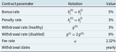
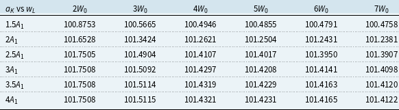
 Aj
 Wj
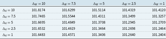
 ΔA
 ΔW
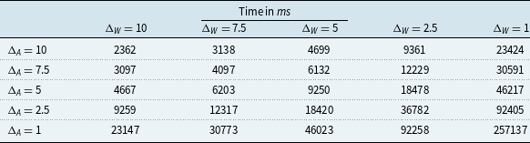
 ΔA
 ΔW
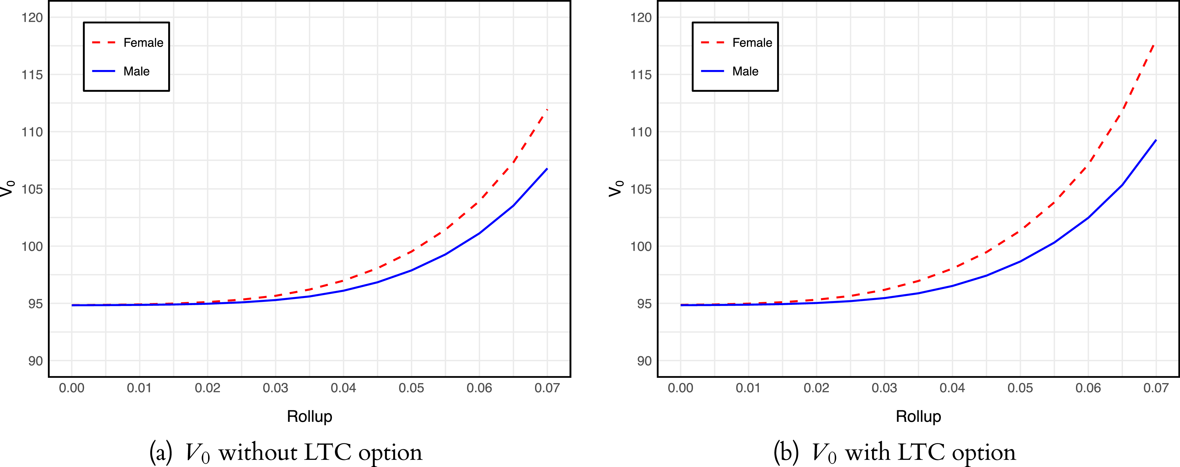
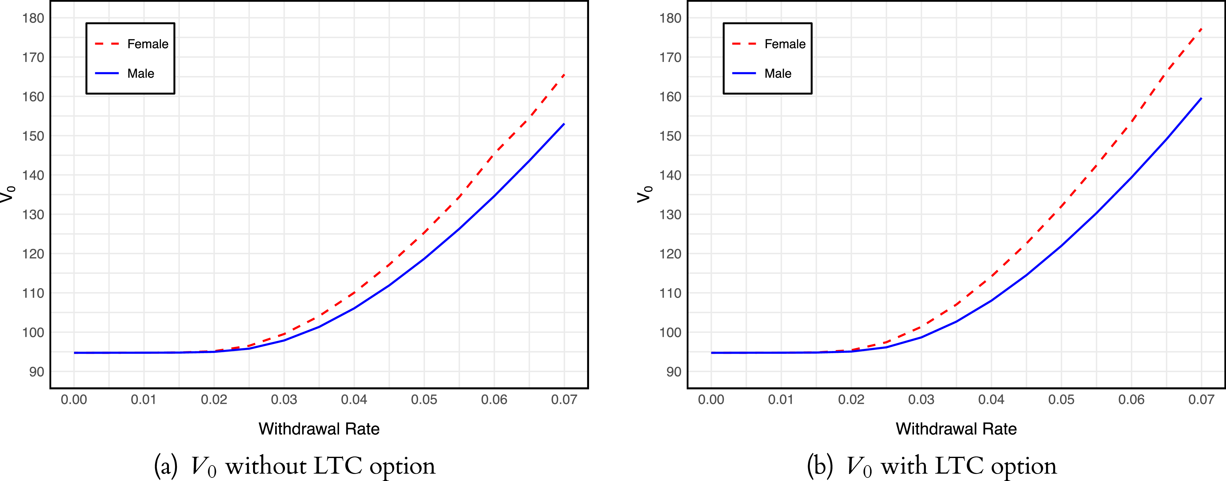
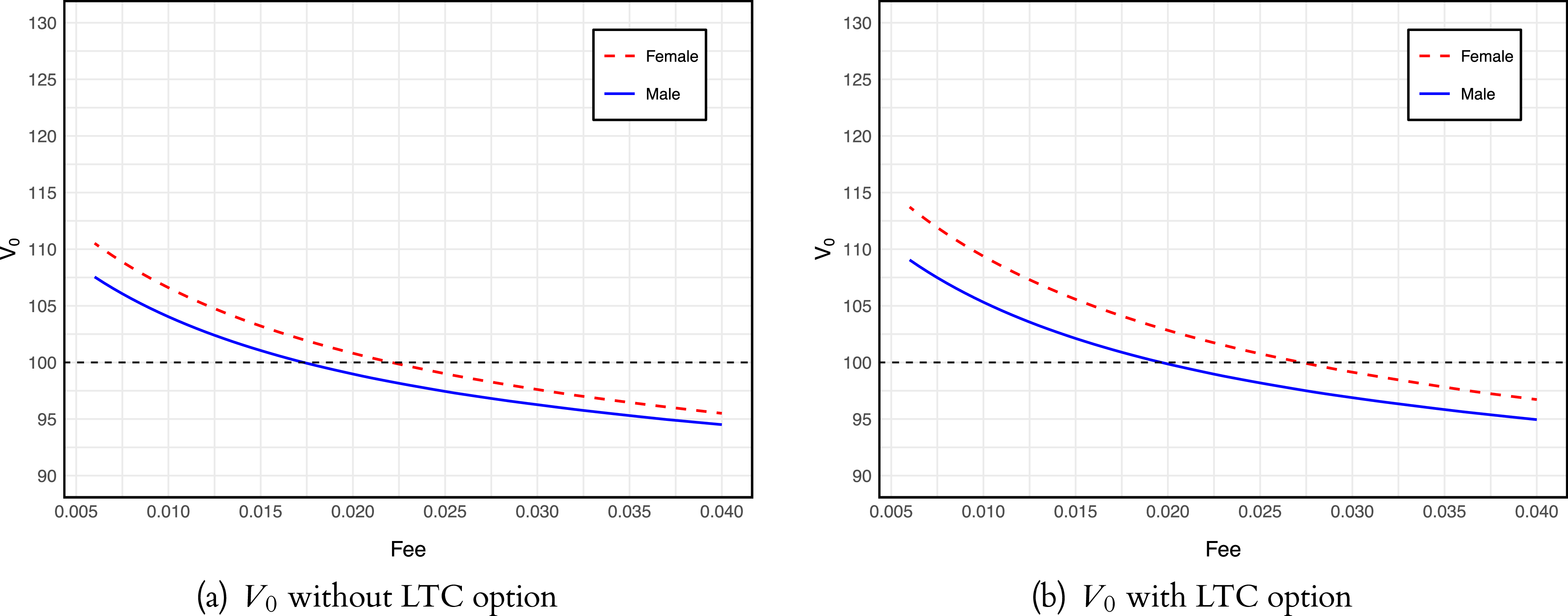
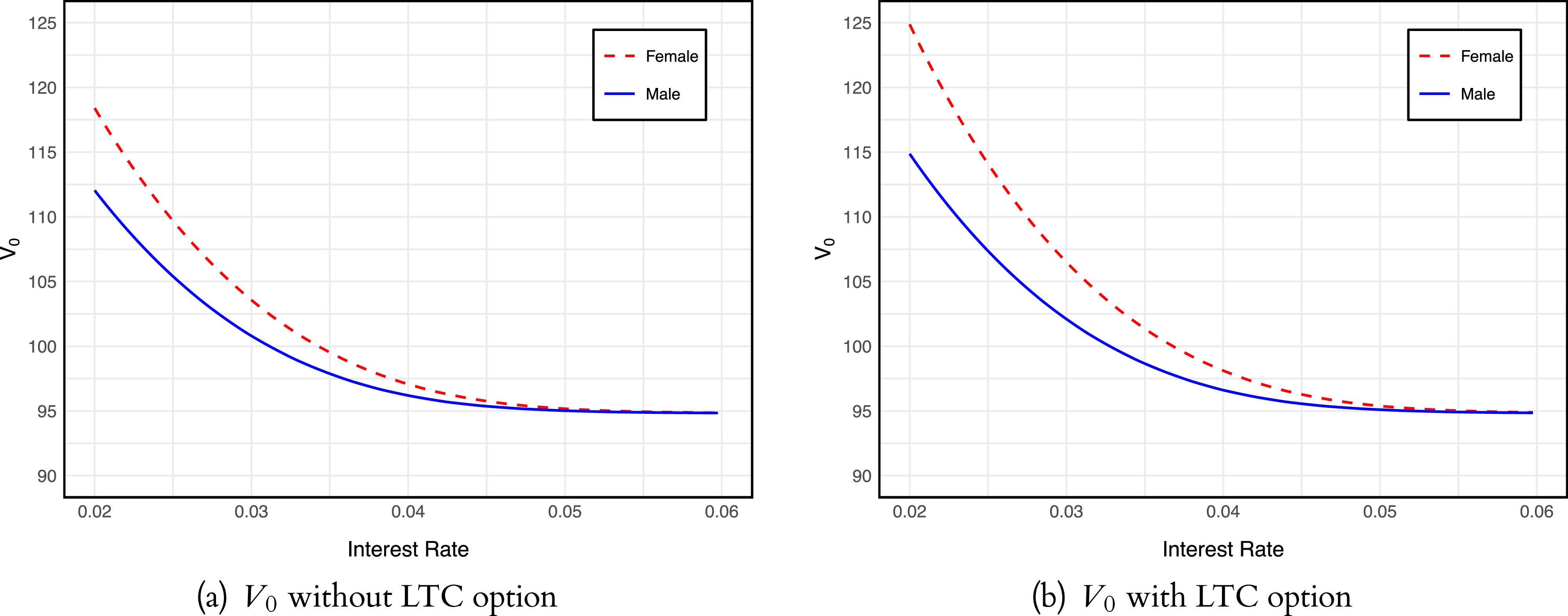

 j=1,5,15
 1
 2
 4

 j=16,20,30
 2
 3
 4
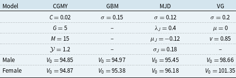
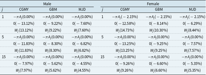
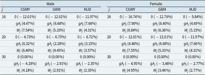
 g
 g(h)

 b

 g
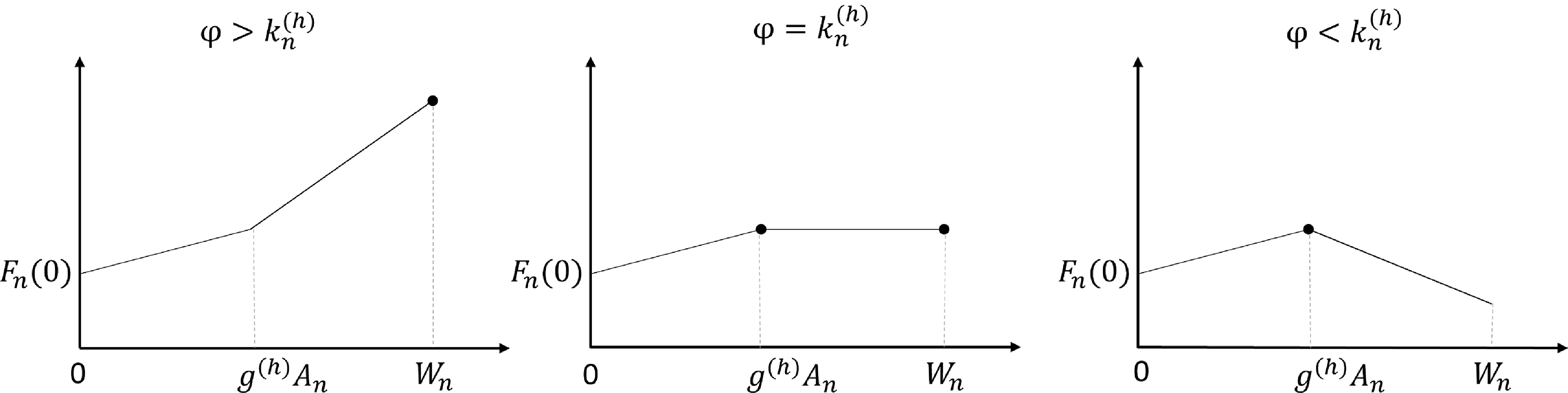
 yn∗∈{g(h)An,Wn}
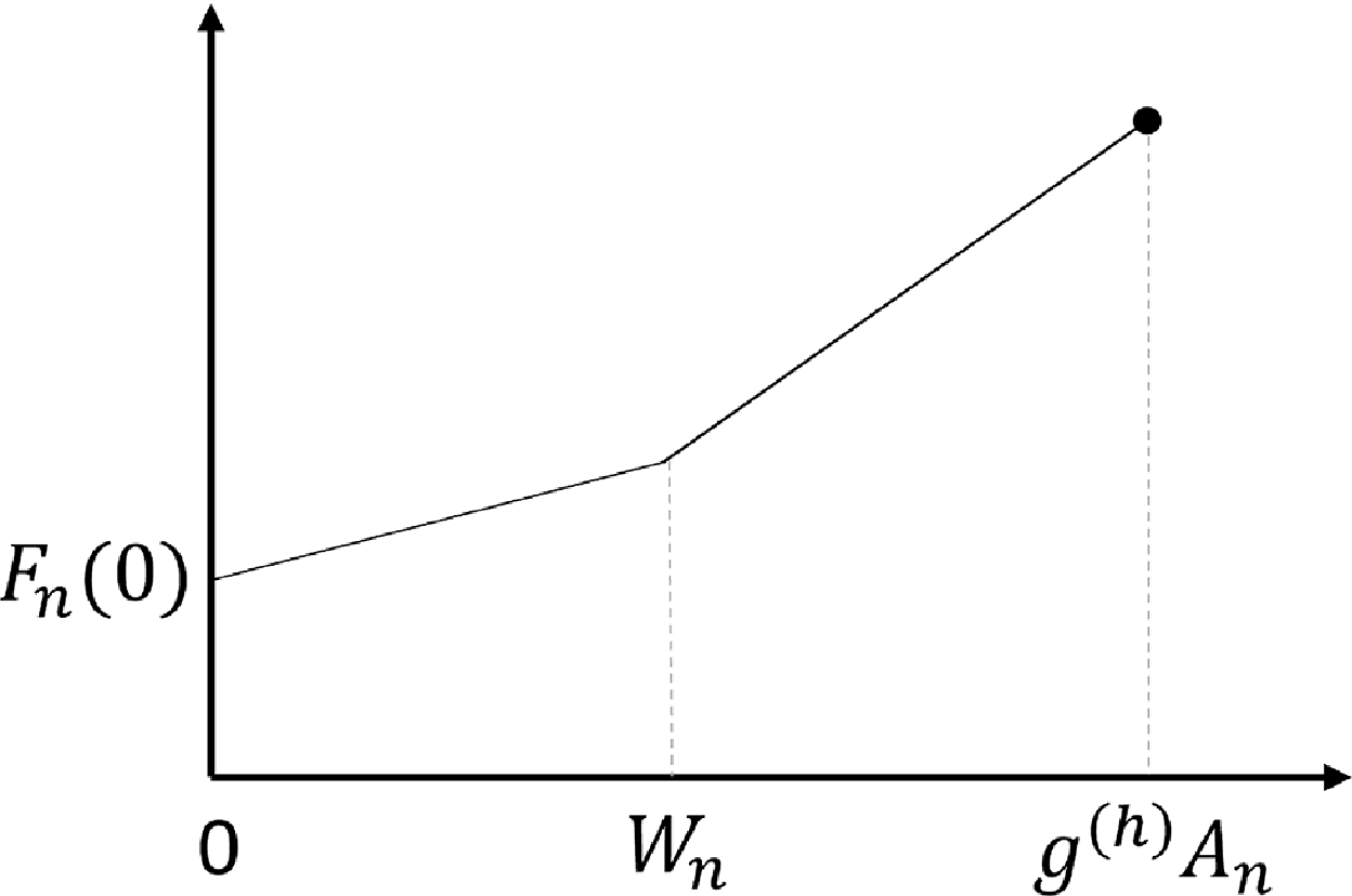
 yn∗=g(h)An
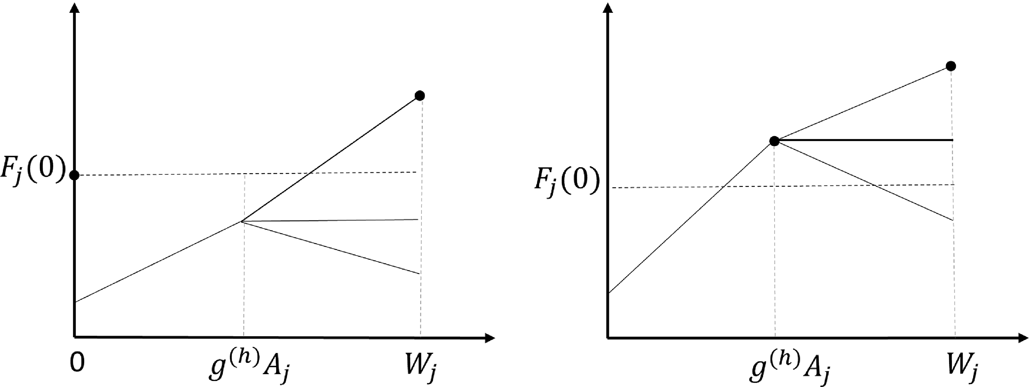
 yj∗∈{0,g(h)Aj,Wj}
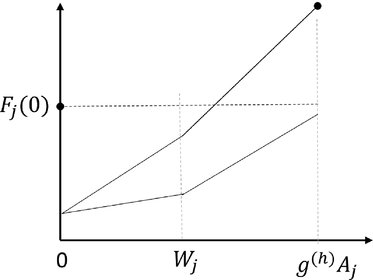
 yj∗∈{0,g(h)Aj}
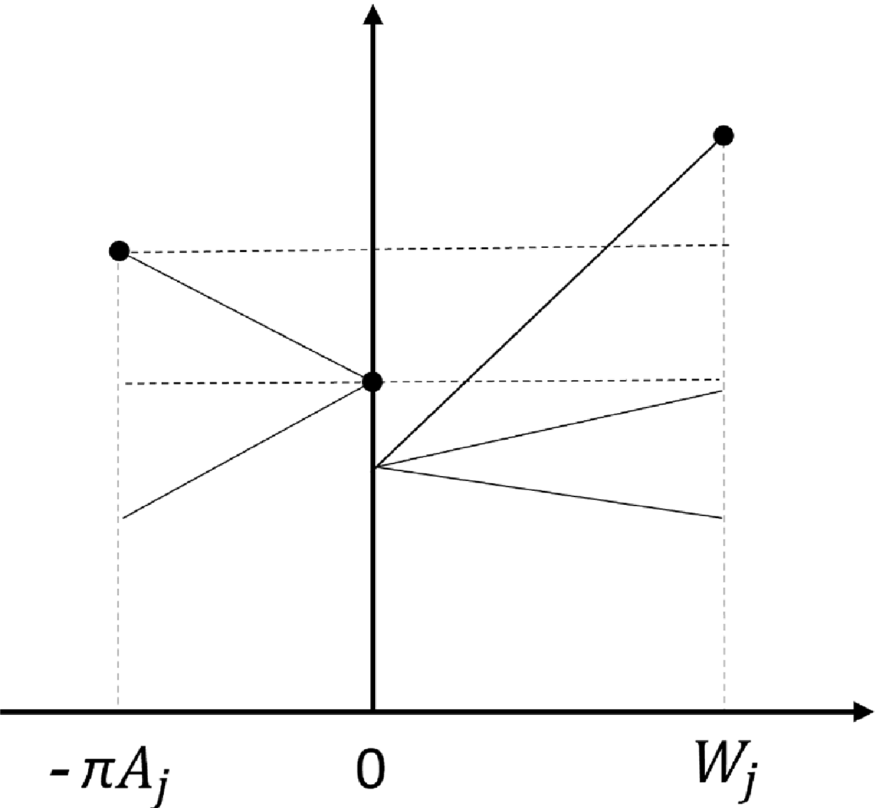
 yj∗∈{−πAj,0,Wj}
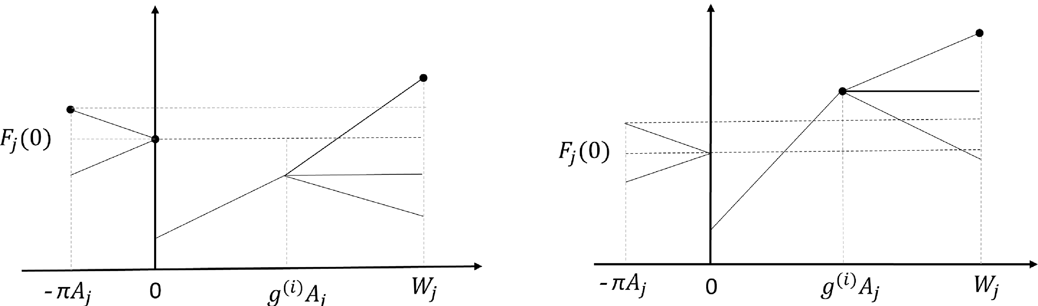
 yj∗∈{−πAj,0,g(i)Aj,Wj}
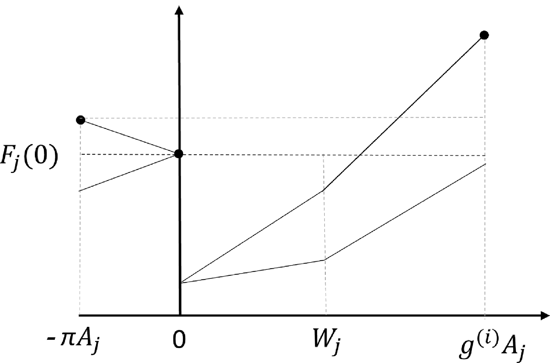
 yj∗∈{−πAj,0,g(i)Aj}


 Open access

