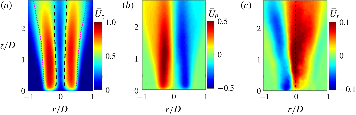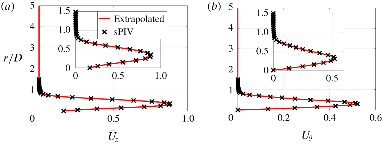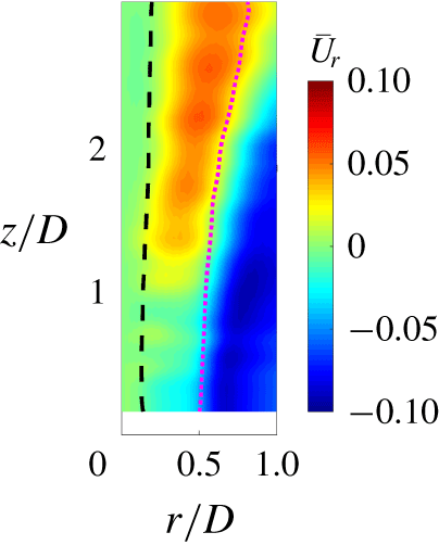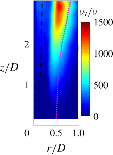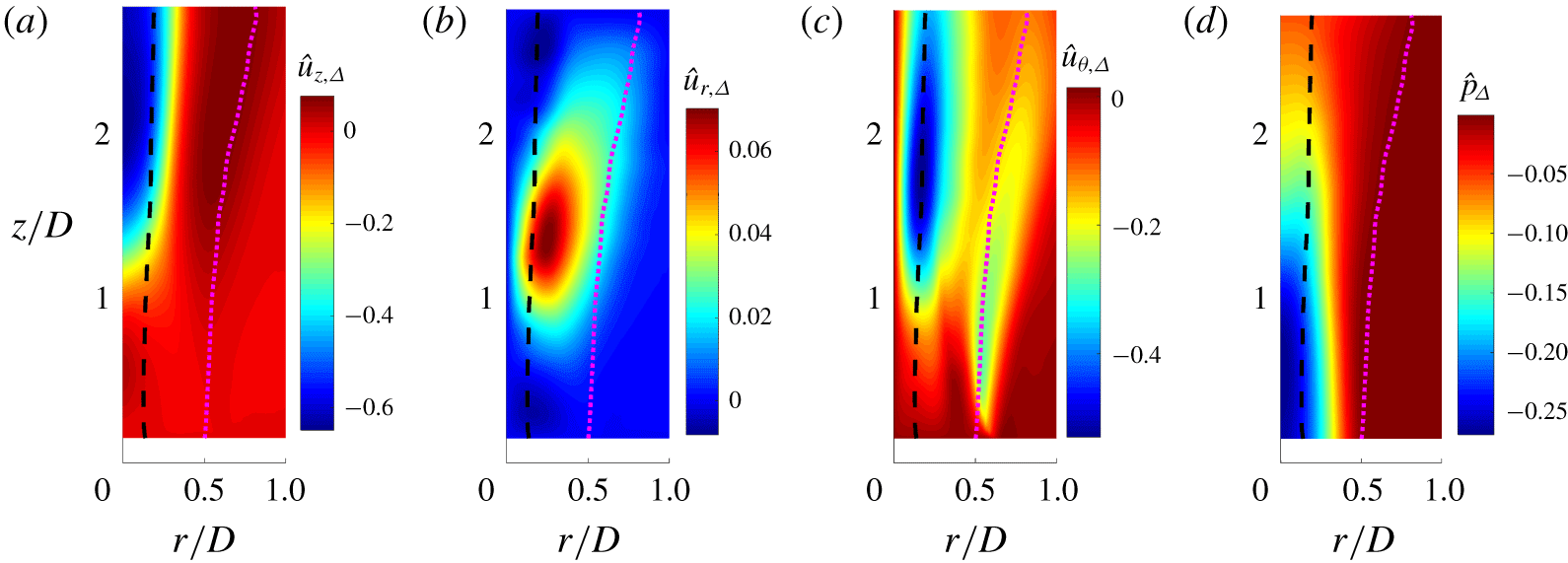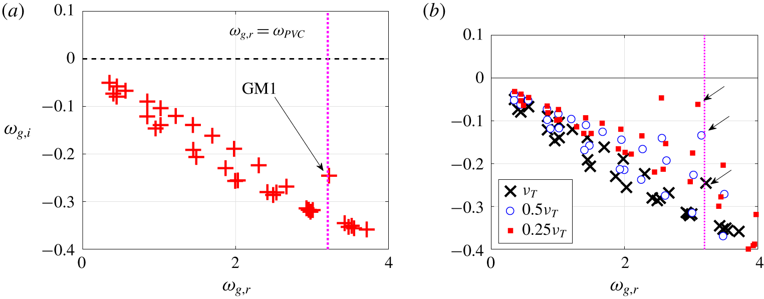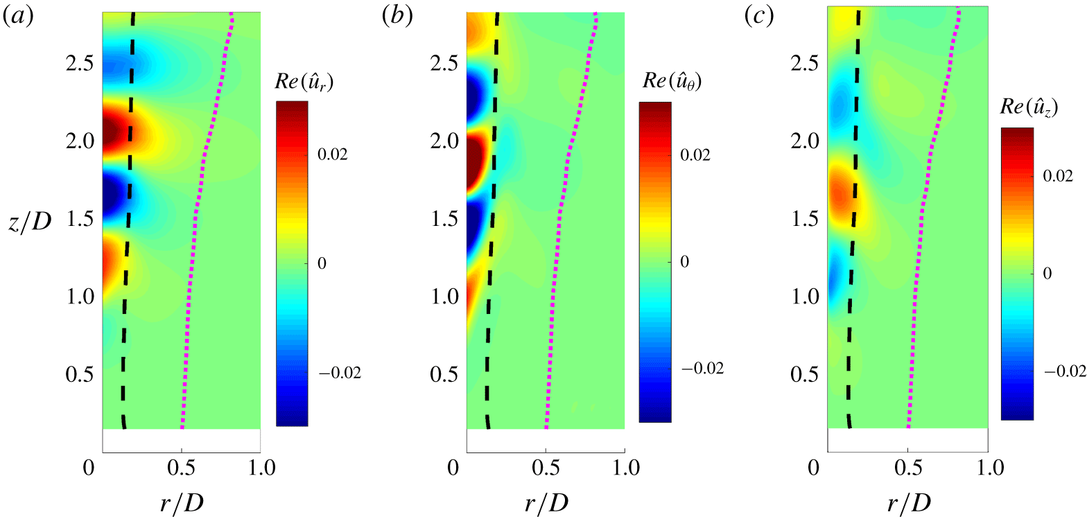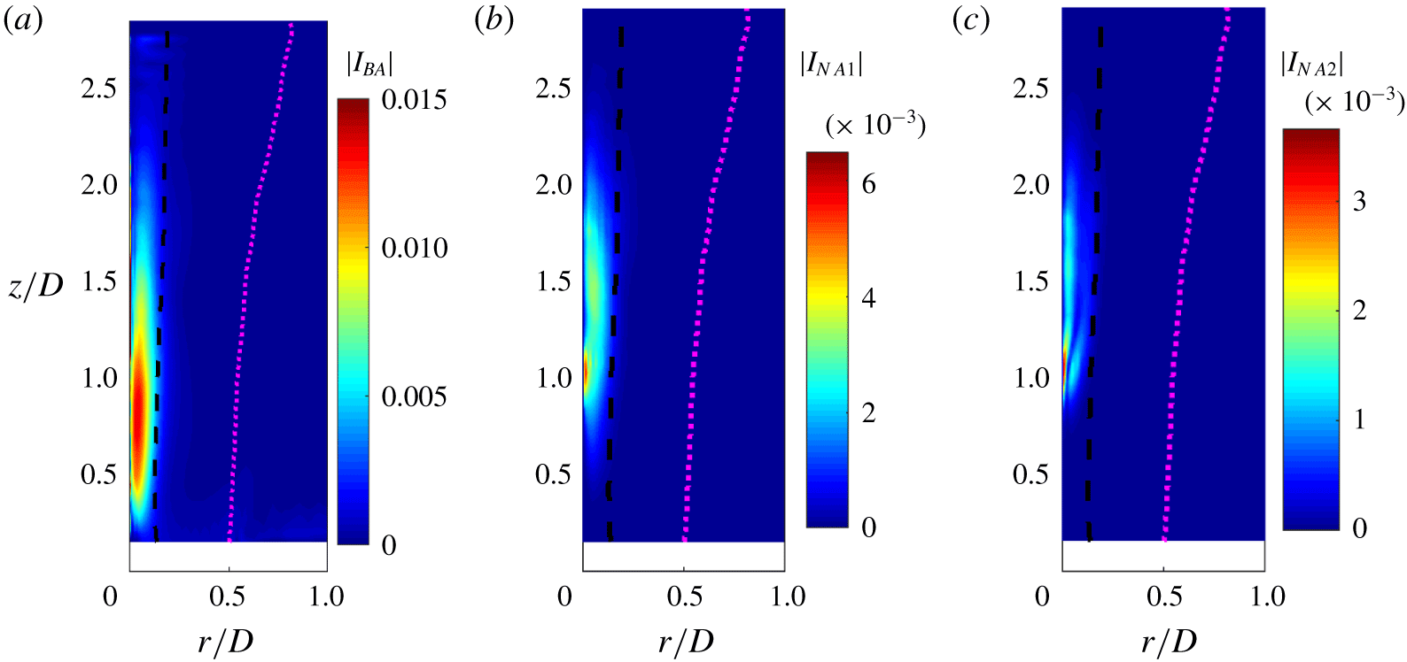


1 Introduction
Swirling flows are technologically significant flows that are generated by imparting an azimuthal velocity component to a nominally streamwise flow. For a sufficiently high ratio of axial fluxes of azimuthal and axial momentum, referred to as the swirl number, various types of structures can appear within the flow due to the breakdown of the axial vortex generated by the swirl. Several types of vortex breakdown have been observed and consequently multiple theories were proposed to explain the phenomenon – see the reviews of Hall (Reference Hall1972), Leibovich (Reference Leibovich1978), Escudier (Reference Escudier1988) and Lucca-Negro & O’Doherty (Reference Lucca-Negro and O’Doherty2001). Vortex breakdown is characterized by the appearance of a central recirculation zone in the flow, in addition to the appearance of coherent unsteady flow oscillations in some cases (Escudier & Keller Reference Escudier and Keller1985; Billant, Chomaz & Huerre Reference Billant, Chomaz and Huerre1998; Liang & Maxworthy Reference Liang and Maxworthy2004, Reference Liang and Maxworthy2005). Several prior experimental studies of jets with variable levels of swirl show the appearance of a self-excited helical vortical structure in the flow accompanied by precession of the recirculation bubble. For this reason, this structure is referred to as precessing vortex core (PVC) (Syred Reference Syred2006) and is distinct from other types of unsteady vortex breakdown modes such as the spiral or the bubble–spiral breakdown mode.
In the context of gas turbine combustors, where swirl is often used to stabilize flames, PVCs can induce changes in the overall shape of the flame sheet (Moeck et al. Reference Moeck, Bourgouin, Durox, Schuller and Candel2012; Taamallah, Shanbhogue & Ghoniem Reference Taamallah, Shanbhogue and Ghoniem2016). This is because the PVC can potentially cause the formation of low velocity regions that, in turn, provide a pathway for flame propagation and therefore flame shape change. These events can potentially then result in the onset of thermoacoustic pressure oscillations (Shanbhogue et al. Reference Shanbhogue, Sanusi, Taamallah, Habib, Mokheimer and Ghoniem2016; Taamallah et al. Reference Taamallah, Shanbhogue and Ghoniem2016). In liquid-fuelled combustors, the PVC can influence the spatio-temporal distribution of fuel droplets resulting from fuel jet atomization, potentially resulting in spatio-temporal inhomogeneities in unburnt mixture composition (see e.g. Renaud, Ducruix & Zimmer Reference Renaud, Ducruix and Zimmer2019). These inhomogeneities, after combustion, can create pockets of relatively high temperature in the combustor flow field and result in an increase in combustor nitrogen oxide emissions. Interaction between high-temperature pockets and the combustor exit can also generate thermoacoustic pressure oscillations in the combustor. These pressure oscillations can potentially result in damage to engine hardware and result in poor combustion efficiency (Lieuwen Reference Lieuwen2012). On the other hand, at other conditions, PVCs can also promote liquid jet atomization and consequently rapid fuel air mixing, thereby serving a beneficial role (Anacleto et al. Reference Anacleto, Fernandes, Heitor and Shtork2003). For all the above reasons, understanding the mechanism governing the onset and sustenance of the PVC oscillation and more generally other hydrodynamic instabilities in swirling flows is necessary. This insight can potentially enable the design of gas turbine combustor fuel nozzles and fuel injection strategies that can appropriately harness flow instabilities to meet low pollutant emission level targets across a range of operating conditions while simultaneously circumventing operability constraints imposed by thermoacoustic oscillations.
The dynamics of swirling jets can, to a large extent, be characterized by the swirl number and the Reynolds number ( $Re$). In this paper, the time-averaged flow field of an unconfined swirling round jet transitions from a weakly swirled round jet state to a fully developed bubble-type vortex breakdown state with increasing swirl. The latter state shows the formation of a recirculation zone on the centreline of the flow, located within a couple of nozzle diameters downstream of the nozzle exit. Previous experiments have reported various kinds of vortex breakdown modes in swirling flows, such as bubble-type vortex breakdown, conical vortex breakdown and spiral vortex breakdown (Sarpkaya Reference Sarpkaya1971a,Reference Sarpkayab; Escudier & Keller Reference Escudier and Keller1985; Billant et al. Reference Billant, Chomaz and Huerre1998). In the present study, a bubble-type vortex breakdown featuring a central recirculation zone (CRZ) is observed (Billant et al. Reference Billant, Chomaz and Huerre1998; Liang & Maxworthy Reference Liang and Maxworthy2004, Reference Liang and Maxworthy2005). Due to the presence of the CRZ, a strong inner shear layer (ISL) is formed between the CRZ and the annular jet. Likewise, an outer shear layer (OSL) is formed between the annular jet and the ambient fluid. Apart from these two shear layers, strong radial variations of azimuthal velocity develop between the central vortex core region and the ambient fluid outside the core. The presence of multiple shear layers, swirl and the central recirculation zone makes the flow field highly susceptible to various hydrodynamic instability driven flow field oscillations (Olendraru et al. Reference Olendraru, Sellier, Rossi and Huerre1999; Loiseleux, Delbende & Huerre Reference Loiseleux, Delbende and Huerre2000; Olendraru & Sellier Reference Olendraru and Sellier2002; Gallaire & Chomaz Reference Gallaire and Chomaz2003b; Oberleithner et al. Reference Oberleithner, Sieber, Nayeri, Paschereit, Petz, Hege, Noack and Wygnanski2011; Juniper Reference Juniper2012; Manoharan et al. Reference Manoharan, Hansford, OConnor and Hemchandra2015; Douglas et al. Reference Douglas, Smith, Emerson, Manoharan, Hemchandra and Lieuwen2018; Muthiah & Samanta Reference Muthiah and Samanta2018; Smith et al. Reference Smith, Douglas, Emerson and Lieuwen2018).
Several studies have focused on understanding coherent oscillations in swirl flows using linear stability analysis. Asymptotic methods, based on Wentzel–Kramers–Brillouin–Jeffreys (WKBJ) expansions, allow the use of results from local hydrodynamic stability analysis to characterize these oscillations for base states slowly evolving in one direction, i.e. a weakly non-parallel base flow (Chomaz, Huerre & Redekopp Reference Chomaz, Huerre and Redekopp1991; Monkewitz, Huerre & Chomaz Reference Monkewitz, Huerre and Chomaz1993). Gallaire et al. (Reference Gallaire, Ruith, Meiburg, Chomaz and Huerre2006) used this approach to study the appearance of vortex breakdown-induced flow oscillations seen in the wake of the recirculation zone seen in the simulations of Ruith et al. (Reference Ruith, Chen, Meiburg and Maxworthy2003). However, WKBJ theory-based methods are limited in their quantitative accuracy when used to analyse the stability of base flows that vary very rapidly in the streamwise direction, as in the case of swirl flows. For this reason, several recent studies have used fully global stability analysis methods that do not rely on the weakly non-parallel assumption. Meliga, Gallaire & Chomaz (Reference Meliga, Gallaire and Chomaz2012) and Qadri, Mistry & Juniper (Reference Qadri, Mistry and Juniper2013) show that unsteady helical oscillations downstream of an axisymmetric breakdown bubble are associated with a globally unstable hydrodynamic mode. Qadri et al. (Reference Qadri, Mistry and Juniper2013) show, from a linear structural sensitivity analysis, that the wavemaker driving these oscillations is located at the upstream end of the breakdown bubble. All the above studies have focused primarily on laminar flows.
Turbulent swirled jets at high swirl intensities feature coherent flow oscillations in the flow field that induce helical precession of the central vortex core about the flow axis and a helical rollup of the shear layers surrounding the breakdown bubble (see for e.g. Escudier & Keller Reference Escudier and Keller1985; Huang & Yang Reference Huang and Yang2009). Turbulent flows can be analysed using the triple decomposition (Reynolds & Hussain Reference Reynolds and Hussain1972) wherein the instantaneous quantities describing the turbulent flow field are decomposed into a time-averaged, coherently oscillating, and incoherent turbulence fluctuations. Tammisola & Juniper (Reference Tammisola and Juniper2016) used this approach to predict the characteristics of PVC oscillations in a turbulent swirling jet produced by a gas turbine injector. Their analysis suggests that global linear stability analysis performed on the time-averaged flow field, with Reynolds stress components modelled using the eddy viscosity hypothesis, predicts the PVC oscillation as a marginally stable helical mode. Further, they demonstrated, from a linear structural sensitivity analysis, that the instability of this mode is driven by the unsteady flow in a region located inside the injector and upstream of the vortex breakdown bubble. Oberleithner et al. (Reference Oberleithner, Sieber, Nayeri, Paschereit, Petz, Hege, Noack and Wygnanski2011) studied the onset of PVC oscillations in a variable swirl round jet at fixed mass flow rate. Their study showed that with increasing levels of swirl, the variation of the amplitude and frequency characteristics of the PVC with swirl intensity suggests the emergence of a stable helical limit cycle in the jet beyond a critical value of swirl number. They also present evidence from local spatial analysis that suggests that the helical shear layer rollup is due to forcing of the shear layers imposed by the PVC oscillations. These studies have provided valuable insight into various aspects of how PVCs may arise in flows with swirl from a linear stability standpoint. However, key questions still remain as follows:
(i) Causality – does the formation of a breakdown bubble (vortex breakdown) cause a PVC or does the PVC cause the former?
(ii) Is the PVC due to the emergence of a stable limit cycle as prior experimental studies suggest (Anacleto et al. Reference Anacleto, Fernandes, Heitor and Shtork2003; Oberleithner et al. Reference Oberleithner, Sieber, Nayeri, Paschereit, Petz, Hege, Noack and Wygnanski2011)?
(iii) When can linear hydrodynamic stability predictions based on time-averaged flows predict PVC frequencies and spatial oscillation amplitude distribution fields with good quantitative accuracy (Tammisola & Juniper Reference Tammisola and Juniper2016)?
Prior studies have presented a variety of experimental observations in variable swirl jets (Escudier & Keller Reference Escudier and Keller1985; Oberleithner et al. Reference Oberleithner, Sieber, Nayeri, Paschereit, Petz, Hege, Noack and Wygnanski2011) and in swirl nozzles with more complicated geometry (Anacleto et al. Reference Anacleto, Fernandes, Heitor and Shtork2003; Tammisola & Juniper Reference Tammisola and Juniper2016) that suggest that all of the above points are indeed true. However, theoretical understanding that directly addresses these questions, to the best of the authors’ knowledge, has still not been presented hitherto.
The present paper makes progress towards improving the theoretical understanding of the three points stated above as follows. We use the method of multiple scales to derive an asymptotic solution for the onset of coherent flow oscillations from the fully nonlinear Navier–Stokes equations. The analysis uses a small parameter,  $\unicode[STIX]{x1D716}\sim (S-S_{c})^{1/2}$. The parameter
 $S$ is an appropriately defined swirl number that captures the intensity of swirl. The value
 $S_{c}$ is the swirl number at which coherent flow oscillations arise. These types of weakly nonlinear analysis have been performed several times in the past in the context of low Reynolds number laminar flows. Sipp & Lebedev (Reference Sipp and Lebedev2007) apply the method of multiple scales to the case of two-dimensional laminar flows that show onset of coherent oscillations with increasing
 $Re$. They directly address the question of usefulness of linear hydrodynamic stability analysis using time-averaged flows as base flows to predict limit-cycle frequency and spatial amplitude distribution characteristics. Meliga et al. (Reference Meliga, Gallaire and Chomaz2012) perform weakly nonlinear analysis with two parameters,
 $S$ and
 $Re$, in order to explain instability mode selection in low
 $Re$ swirling flows. Recently, Rigas, Morgans & Morrison (Reference Rigas, Morgans and Morrison2017) applied a weakly nonlinear analysis to understand the response of a turbulent wake behind an axisymmetric bluff body to imposed forcing. They show that the mathematical structure of equations governing flow oscillation amplitudes in laminar studies carries over to the turbulent regime when appropriate turbulence modelling assumptions are introduced.
We apply the weakly nonlinear theory derived in this paper to understand the emergence of PVC oscillations in a constant mass flow rate, variable swirl jet experiment at  $Re=59\,000$ (based on the jet diameter and bulk flow velocity) (Clees et al. Reference Clees, Lewalle, Frederick and O’Connor2018; Frederick et al. Reference Frederick, Manoharan, Dudash, Brubaker, Hemchandra and O’Connor2018). Time-resolved velocity field measurements are obtained using stereoscopic particle image velocimetry (sPIV) over a range of swirl numbers. The onset of PVC oscillations is observed at
 $S_{c}=0.61$. We model the impact of turbulent transport using an eddy viscosity model and derive the Stuart–Landau equation governing the oscillation amplitude of coherent flow oscillations. The analysis yields closed-form analytical expressions for the coefficients in this equation that control the strength of the linear growth term and the nonlinear saturation term. These are expressed in terms of the helical linear eigenmode oscillating with the PVC frequency at
 $S_{c}$, functions that describe the modification of the base flow for
 $S>S_{c}$ and the spatial amplitude distribution of the flow oscillations at the first harmonic of the PVC.
We determine these coefficients for the present jet experiments using only the time-averaged flow field at  $S_{c}$ as an input to these calculations. The numerical values of the coefficients of our Stuart–Landau equation confirm that the PVC is indeed the result of a supercritical Hopf bifurcation in the flow state at
 $S_{c}$. Prior studies presume this fact based on characteristics observed in the experiment (Oberleithner et al. Reference Oberleithner, Sieber, Nayeri, Paschereit, Petz, Hege, Noack and Wygnanski2011; Rigas et al. Reference Rigas, Morgans and Morrison2017).
Further, we can identify individual contributions to the nonlinear saturation coefficient in the Stuart–Landau equation from base flow distortion and harmonic generation. Determining the numerical values for these two individual contributions allows us to conclude, based on the analysis of Sipp & Lebedev (Reference Sipp and Lebedev2007), that linear hydrodynamic stability analysis using the time-averaged flow field for  $S>S_{c}$ can indeed yield quantitatively accurate estimates of PVC frequencies and spatial amplitude distributions in swirled jets.
Further, our analysis yields an equation for the base-flow modification function that describes the impact that increasing  $S$ beyond
 $S_{c}$ has on the time-averaged flow at
 $S_{c}$. Our analysis shows that, in general, this quantity is independent of the characteristics of the hydrodynamic instability modes of the flow. For the present jet experiment, the base-flow modification shows that increasing
 $S$ beyond
 $S_{c}$ induces the formation of a recirculation zone on the flow centreline, i.e. a steady bubble-type breakdown of the axial vortex in the flow. Thus, the dependence of the linear growth term coefficient in the Stuart–Landau equation on the base-flow modification function shows that the PVC is a hydrodynamic instability that is caused by the change in flow structure due to vortex breakdown and that the converse is not the case, thereby clarifying the causality question mentioned earlier. To the best of our knowledge, prior studies of swirled jets do not provide the insights summarized above, which are the principal contributions of this paper determined ab initio from the time-averaged based flow at
 $S_{c}$.
The rest of this paper is organized as follows. Section 2 discusses the theoretical formulation used for performing global stability and weakly nonlinear analysis. Section 3 explains the experimental set-up used in the present study. Section 4 discusses the time-averaged and unsteady flow characteristics at various swirl intensities. Section 5 describes the numerical methods and base flow used to compute various results from § 2, for the present swirling jet experiment. Section 6 presents the results obtained from global and weakly nonlinear analysis. Section 7 concludes the paper with an overview of current findings and future work.
2 Theoretical formulation
We first derive the governing equations for the coherent unsteady component of an unconfined, nominally axisymmetric constant-density swirling turbulent jet. The equations are formulated in cylindrical coordinates  $(r,\unicode[STIX]{x1D703},z)$ with the
 $z$-axis aligned along the streamwise flow direction. Radial (
 $u_{r}$) and axial (
 $u_{z}$) velocity components are expressed in non-dimensional form using a suitably chosen reference velocity,
 $U_{z,ref}$. Likewise, the azimuthal (
 $u_{\unicode[STIX]{x1D703}}$) velocity component is non-dimensionalized using a suitably chosen reference velocity
 $U_{\unicode[STIX]{x1D703},ref}$. A reference length scale
 $l_{ref}$ is chosen to non-dimensionalize all lengths. Thus, the Navier–Stokes equations for constant density swirling flows in operator form can be written as follows:
 $$\begin{eqnarray}{\mathcal{B}}^{s}\frac{\unicode[STIX]{x2202}\boldsymbol{q}}{\unicode[STIX]{x2202}t}+{\mathcal{N}}\{\boldsymbol{q}\}\boldsymbol{q}+S{\mathcal{N}}^{s}\{\boldsymbol{q}\}\boldsymbol{q}+S^{2}{\mathcal{N}}^{ss}\{\boldsymbol{q}\}\boldsymbol{q}={\mathcal{L}}_{v}\boldsymbol{q}+S{\mathcal{L}}_{v}^{s}\boldsymbol{q},\end{eqnarray}$$
where  $\boldsymbol{q}=[u_{r},u_{\unicode[STIX]{x1D703}},u_{z},p]^{\text{T}}$ is the vector of flow variables comprised of the three velocity components and pressure. The operators
 ${\mathcal{N}}\{\boldsymbol{q}\}$,
 ${\mathcal{N}}^{s}\{\boldsymbol{q}\}$ and
 ${\mathcal{N}}^{ss}\{\boldsymbol{q}\}$ are nonlinear operators representing the convective terms in the governing equations. The vector within ‘
 $\{\}$’ is used to denote the fact that the nonlinear operators are functions of flow variables. The linear operators
 ${\mathcal{L}}_{v}$ and
 ${\mathcal{L}}_{v}^{s}$ contain the viscous and the pressure gradient terms. The details of these operators in matrix form are given in appendix A. The quantity
 $S=U_{\unicode[STIX]{x1D703},ref}/U_{z,ref}$ is the swirl number. The operator
 ${\mathcal{B}}^{s}$ is a diagonal matrix:
 ${\mathcal{B}}^{s}=\text{diag}(1,S,1,0)$.
We next introduce the triple decomposition where the instantaneous flow variables are decomposed into an axisymmetric time-averaged component,  $\bar{\boldsymbol{Q}}=[\bar{U}_{r},\bar{U}_{\unicode[STIX]{x1D703}},\bar{U}_{z},\bar{P}]^{\text{T}}$, a coherent fluctuation component,
 $\boldsymbol{q}_{c}^{\prime }=[u_{r}^{\prime },u_{\unicode[STIX]{x1D703}}^{\prime },u_{z}^{\prime },p^{\prime }]^{\text{T}}$, and an incoherent turbulent fluctuation component,
 $\boldsymbol{q}^{\prime \prime }=[u_{r}^{\prime \prime },u_{\unicode[STIX]{x1D703}}^{\prime \prime },u_{z}^{\prime \prime },p^{\prime \prime }]^{\text{T}}$, as follows (Reynolds & Hussain Reference Reynolds and Hussain1972):
 $$\begin{eqnarray}\boldsymbol{q}(r,\unicode[STIX]{x1D703},z,t)=\bar{\boldsymbol{Q}}(r,z)+\boldsymbol{q}_{c}^{\prime }(r,\unicode[STIX]{x1D703},z,t)+\boldsymbol{q}^{\prime \prime }(r,\unicode[STIX]{x1D703},z,t).\end{eqnarray}$$
Using equation (2.2) in (2.1) and time averaging yields the governing equations for  $\bar{\boldsymbol{Q}}$ as follows:
 $$\begin{eqnarray}\displaystyle & & \displaystyle {\mathcal{N}}\{\bar{\boldsymbol{Q}}\}\bar{\boldsymbol{Q}}+\overline{{\mathcal{N}}\{\boldsymbol{q}_{c}^{\prime }\}\boldsymbol{q}_{c}^{\prime }}+\overline{{\mathcal{N}}\{\boldsymbol{q}^{\prime \prime }\}\boldsymbol{q}^{\prime \prime }}+S\left({\mathcal{N}}^{s}\{\bar{\boldsymbol{Q}}\}\bar{\boldsymbol{Q}}+\overline{{\mathcal{N}}^{s}\{\boldsymbol{q}_{c}^{\prime }\}\boldsymbol{q}_{c}^{\prime }}+\overline{{\mathcal{N}}^{s}\{\boldsymbol{q}^{\prime \prime }\}\boldsymbol{q}^{\prime \prime }}\right)\nonumber\\ \displaystyle & & \displaystyle \quad +\,S^{2}\left({\mathcal{N}}^{ss}\{\bar{\boldsymbol{Q}}\}\bar{\boldsymbol{Q}}+\overline{{\mathcal{N}}^{ss}\{\boldsymbol{q}_{c}^{\prime }\}\boldsymbol{q}_{c}^{\prime }}+\overline{{\mathcal{N}}^{ss}\{\boldsymbol{q}^{\prime \prime }\}\boldsymbol{q}^{\prime \prime }}\right)={\mathcal{L}}_{v}\bar{\boldsymbol{Q}}+S{\mathcal{L}}_{v}^{s}\bar{\boldsymbol{Q}},\end{eqnarray}$$
where the terms in overbars represent the contribution to time-averaged momentum transport from coherent and incoherent fluctuations. Following prior studies by Oberleithner et al. (Reference Oberleithner, Stöhr, Im, Arndt and Steinberg2015), Rukes, Paschereit & Oberleithner (Reference Rukes, Paschereit and Oberleithner2016) and Tammisola & Juniper (Reference Tammisola and Juniper2016), we use the eddy viscosity hypothesis, which relates these terms linearly to the time-averaged rates of strain in a Newtonian fashion via a turbulent viscosity coefficient ( $\unicode[STIX]{x1D708}_{T}$) (see appendix B). Thus, all of these terms in (2.3) can now be written symbolically in terms of two new operators as follows:
 $$\begin{eqnarray}{\mathcal{N}}\{\bar{\boldsymbol{Q}}\}\bar{\boldsymbol{Q}}+S{\mathcal{N}}^{s}\{\bar{\boldsymbol{Q}}\}\bar{\boldsymbol{Q}}+S^{2}{\mathcal{N}}^{ss}\{\bar{\boldsymbol{Q}}\}\bar{\boldsymbol{Q}}={\mathcal{L}}_{T}\bar{\boldsymbol{Q}}+S{\mathcal{L}}_{T}^{s}\bar{\boldsymbol{Q}},\end{eqnarray}$$
where  ${\mathcal{L}}_{T}$ and
 ${\mathcal{L}}_{T}^{s}$ include contributions from both molecular transport and eddy viscosity model terms (see (A 6)–(A 7)).
Next, substituting (2.2) into (2.1) and phase averaging yields the evolution equations for the coherent flow component  $\tilde{\boldsymbol{q}}=\bar{\boldsymbol{Q}}+\boldsymbol{q}_{c}^{\prime }$ as follows:
 $$\begin{eqnarray}\displaystyle & & \displaystyle {\mathcal{B}}^{s}\frac{\unicode[STIX]{x2202}\tilde{\boldsymbol{q}}}{\unicode[STIX]{x2202}t}+{\mathcal{N}}\{\tilde{\boldsymbol{q}}\}\tilde{\boldsymbol{q}}+\widetilde{{\mathcal{N}}\{\boldsymbol{q}^{\prime \prime }\}\boldsymbol{q}^{\prime \prime }}+S\left({\mathcal{N}}^{s}\{\tilde{\boldsymbol{q}}\}\tilde{\boldsymbol{q}}+\widetilde{{\mathcal{N}}^{s}\{\boldsymbol{q}^{\prime \prime }\}\boldsymbol{q}^{\prime \prime }}\right)\nonumber\\ \displaystyle & & \displaystyle \quad +\,S^{2}\left({\mathcal{N}}^{ss}\{\tilde{\boldsymbol{q}}\}\tilde{\boldsymbol{q}}+\widetilde{{\mathcal{N}}^{ss}\{\boldsymbol{q}^{\prime \prime }\}\boldsymbol{q}^{\prime \prime }}\right)={\mathcal{L}}_{v}\tilde{\boldsymbol{q}}+S{\mathcal{L}}_{v}^{s}\tilde{\boldsymbol{q}}.\end{eqnarray}$$
Subtracting (2.3) from (2.5) yields the evolution equations for ( $\boldsymbol{q}_{c}^{\prime }$) as follows:
 $$\begin{eqnarray}\displaystyle & & \displaystyle {\mathcal{B}}^{s}\frac{\unicode[STIX]{x2202}\boldsymbol{q}_{c}^{\prime }}{\unicode[STIX]{x2202}t}+{\mathcal{N}}\{\bar{\boldsymbol{Q}}\}\boldsymbol{q}_{c}^{\prime }+{\mathcal{N}}\{\boldsymbol{q}_{c}^{\prime }\}\bar{\boldsymbol{Q}}+{\mathcal{N}}\{\boldsymbol{q}_{c}^{\prime }\}\boldsymbol{q}_{c}^{\prime }+\widetilde{{\mathcal{N}}\{\boldsymbol{q}^{\prime \prime }\}\boldsymbol{q}^{\prime \prime }}-\overline{{\mathcal{N}}\{\boldsymbol{q}_{c}^{\prime }\}\boldsymbol{q}_{c}^{\prime }}\nonumber\\ \displaystyle & & \displaystyle \quad -\,\overline{{\mathcal{N}}\{\boldsymbol{q}^{\prime \prime }\}\boldsymbol{q}^{\prime \prime }}+S\left({\mathcal{N}}^{s}\{\bar{\boldsymbol{Q}}\}\boldsymbol{q}_{c}^{\prime }+{\mathcal{N}}^{s}\{\boldsymbol{q}_{c}^{\prime }\}\bar{\boldsymbol{Q}}+{\mathcal{N}}^{s}\{\boldsymbol{q}_{c}^{\prime }\}\boldsymbol{q}_{c}^{\prime }+\widetilde{{\mathcal{N}}^{s}\{\boldsymbol{q}^{\prime \prime }\}\boldsymbol{q}^{\prime \prime }}-\overline{{\mathcal{N}}^{s}\{\boldsymbol{q}_{c}^{\prime }\}\boldsymbol{q}_{c}^{\prime }}\right.\nonumber\\ \displaystyle & & \displaystyle \quad -\left.\overline{{\mathcal{N}}^{s}\{\boldsymbol{q}^{\prime \prime }\}\boldsymbol{q}^{\prime \prime }}\vphantom{\widetilde{{\mathcal{N}}^{s}\{\boldsymbol{q}^{\prime \prime }\}\boldsymbol{q}^{\prime \prime }}}\right)+S^{2}\left({\mathcal{N}}^{ss}\{\bar{\boldsymbol{Q}}\}\boldsymbol{q}_{c}^{\prime }+{\mathcal{N}}^{ss}\{\boldsymbol{q}_{c}^{\prime }\}\bar{\boldsymbol{Q}}+{\mathcal{N}}^{ss}\{\boldsymbol{q}_{c}^{\prime }\}\boldsymbol{q}_{c}^{\prime }+\widetilde{{\mathcal{N}}^{ss}\{\boldsymbol{q}^{\prime \prime }\}\boldsymbol{q}^{\prime \prime }}\right.\nonumber\\ \displaystyle & & \displaystyle \quad -\left.\overline{{\mathcal{N}}^{ss}\{\boldsymbol{q}_{c}^{\prime }\}\boldsymbol{q}_{c}^{\prime }}-\overline{{\mathcal{N}}^{ss}\{\boldsymbol{q}^{\prime \prime }\}\boldsymbol{q}^{\prime \prime }}\vphantom{\widetilde{{\mathcal{N}}^{s}\{\boldsymbol{q}^{\prime \prime }\}\boldsymbol{q}^{\prime \prime }}}\right)={\mathcal{L}}_{v}\boldsymbol{q}_{c}^{\prime }+S{\mathcal{L}}_{v}^{s}\boldsymbol{q}_{c}^{\prime }.\end{eqnarray}$$
The difference between phase-averaged and time-averaged nonlinear terms in (2.6) represents the quantitative contribution of coherent fluctuating momentum transport by turbulence fluctuations. Again, we model these terms in terms of the coherent fluctuating rates of strain using the same  $\unicode[STIX]{x1D708}_{T}$ that was used to model turbulent transport terms in (2.3). Therefore, these terms can now be replaced with
 ${\mathcal{L}}_{T}$ and
 ${\mathcal{L}}_{T}^{s}$ operators acting on coherent fluctuating quantities as follows:
 $$\begin{eqnarray}\displaystyle & & \displaystyle {\mathcal{B}}^{s}\frac{\unicode[STIX]{x2202}\boldsymbol{q}_{c}^{\prime }}{\unicode[STIX]{x2202}t}+{\mathcal{N}}\{\bar{\boldsymbol{Q}}\}\boldsymbol{q}_{c}^{\prime }+{\mathcal{N}}\{\boldsymbol{q}_{c}^{\prime }\}\bar{\boldsymbol{Q}}+{\mathcal{N}}\{\boldsymbol{q}_{c}^{\prime }\}\boldsymbol{q}_{c}^{\prime }+S\left({\mathcal{N}}^{s}\{\bar{\boldsymbol{Q}}\}\boldsymbol{q}_{c}^{\prime }+{\mathcal{N}}^{s}\{\boldsymbol{q}_{c}^{\prime }\}\bar{\boldsymbol{Q}}+{\mathcal{N}}^{s}\{\boldsymbol{q}_{c}^{\prime }\}\boldsymbol{q}_{c}^{\prime }\right)\nonumber\\ \displaystyle & & \displaystyle \quad +\,S^{2}\left({\mathcal{N}}^{ss}\{\bar{\boldsymbol{Q}}\}\boldsymbol{q}_{c}^{\prime }+{\mathcal{N}}^{ss}\{\boldsymbol{q}_{c}^{\prime }\}\bar{\boldsymbol{Q}}+{\mathcal{N}}^{ss}\{\boldsymbol{q}_{c}^{\prime }\}\boldsymbol{q}_{c}^{\prime }\right)={\mathcal{L}}_{T}\boldsymbol{q}_{c}^{\prime }+S{\mathcal{L}}_{T}^{s}\boldsymbol{q}_{c}^{\prime }.\end{eqnarray}$$
We add (2.7) and (2.4) to obtain the evolution equation for the total coherent component  $\tilde{\boldsymbol{q}}=\bar{\boldsymbol{Q}}+\boldsymbol{q}_{c}^{\prime }$ as follows:
 $$\begin{eqnarray}{\mathcal{B}}^{s}\frac{\unicode[STIX]{x2202}\tilde{\boldsymbol{q}}}{\unicode[STIX]{x2202}t}+{\mathcal{N}}\{\tilde{\boldsymbol{q}}\}\tilde{\boldsymbol{q}}+S{\mathcal{N}}^{s}\{\tilde{\boldsymbol{q}}\}\tilde{\boldsymbol{q}}+S^{2}{\mathcal{N}}^{ss}\{\tilde{\boldsymbol{q}}\}\tilde{\boldsymbol{q}}={\mathcal{L}}_{T}\tilde{\boldsymbol{q}}+S{\mathcal{L}}_{T}^{s}\tilde{\boldsymbol{q}}.\end{eqnarray}$$
2.1 Weakly nonlinear analysis
The parameter  $S$ in (2.8) is chosen as the control parameter that is varied to change the characteristics of the flow. We presume that there exists a critical swirl number,
 $S_{c}$, beyond which the flow transitions from a stable steady state for
 $S<S_{c}$ to an unsteady state for
 $S>S_{c}$. We determine the characteristics of this unsteady state for small deviations of
 $S$ from
 $S_{c}$ when compared to the flow oscillation amplitude, as follows:
 $$\begin{eqnarray}S=S_{c}+\unicode[STIX]{x1D6E5}_{s}\unicode[STIX]{x1D716}^{2},\end{eqnarray}$$
where  $\unicode[STIX]{x1D716}$ is the normalized amplitude of the unsteady state for
 $S>S_{c}$ and
 $\unicode[STIX]{x1D6E5}_{s}\sim O(1)$. Thus, the matrix
 ${\mathcal{B}}^{s}$ in (2.8) can be written as
 $$\begin{eqnarray}{\mathcal{B}}^{s}={\mathcal{B}}+\unicode[STIX]{x1D6E5}_{s}\unicode[STIX]{x1D716}^{2}{\mathcal{B}}_{1},\end{eqnarray}$$
where  ${\mathcal{B}}=\text{diag}(1,S_{c},1,0)$ and
 ${\mathcal{B}}_{1}=\text{diag}(0,1,0,0)$.
We also presume that the unsteady solution can be characterized by a combination of variations over a ‘fast’ time scale  $t_{1}=t$ and a ‘slow’ time scale
 $t_{2}=\unicode[STIX]{x1D716}^{2}t$. Thus,
 $\tilde{\boldsymbol{q}}$ is now expressed as an asymptotic series in terms of
 $\unicode[STIX]{x1D716}$ as follows:
 $$\begin{eqnarray}\displaystyle \tilde{\boldsymbol{q}}(r,\unicode[STIX]{x1D703},z,t_{1},t_{2}) & = & \displaystyle \boldsymbol{q}_{o}(r,z)+\unicode[STIX]{x1D716}\boldsymbol{q}_{1}(r,\unicode[STIX]{x1D703},z,t_{1},t_{2})+\unicode[STIX]{x1D716}^{2}\boldsymbol{q}_{2}(r,\unicode[STIX]{x1D703},z,t_{1},t_{2})\nonumber\\ \displaystyle & & \displaystyle +\,\unicode[STIX]{x1D716}^{3}\boldsymbol{q}_{3}(r,\unicode[STIX]{x1D703},z,t_{1},t_{2})+\cdots \,,\end{eqnarray}$$
where we have assumed that the contributions to  $\tilde{\boldsymbol{q}}$ at each order depend on both time scales. Each of the nonlinear operators in (2.8) can be expanded in powers of
 $\unicode[STIX]{x1D716}$ as follows:
 $$\begin{eqnarray}\displaystyle & {\mathcal{N}}\{\boldsymbol{q}\}={\mathcal{N}}\{\boldsymbol{q}_{o}\}+\unicode[STIX]{x1D716}{\mathcal{N}}\{\boldsymbol{q}_{1}\}+\unicode[STIX]{x1D716}^{2}{\mathcal{N}}\{\boldsymbol{q}_{2}\}+\cdots \,, & \displaystyle\end{eqnarray}$$
 $$\begin{eqnarray}\displaystyle & {\mathcal{N}}^{s}\{\boldsymbol{q}\}={\mathcal{N}}^{s}\{\boldsymbol{q}_{o}\}+\unicode[STIX]{x1D716}{\mathcal{N}}^{s}\{\boldsymbol{q}_{1}\}+\unicode[STIX]{x1D716}^{2}{\mathcal{N}}^{s}\{\boldsymbol{q}_{2}\}+\cdots \,, & \displaystyle\end{eqnarray}$$
 $$\begin{eqnarray}\displaystyle & {\mathcal{N}}^{ss}\{\boldsymbol{q}\}={\mathcal{N}}^{ss}\{\boldsymbol{q}_{o}\}+\unicode[STIX]{x1D716}{\mathcal{N}}^{ss}\{\boldsymbol{q}_{1}\}+\unicode[STIX]{x1D716}^{2}{\mathcal{N}}^{ss}\{\boldsymbol{q}_{2}\}+\cdots \,. & \displaystyle\end{eqnarray}$$
Substituting (2.9) and (2.11)–(2.14) into (2.8), yields the following equation at  $O(1)$:
 $$\begin{eqnarray}\displaystyle {\mathcal{N}}\{\boldsymbol{q}_{o}\}\boldsymbol{q}_{o}+S_{c}{\mathcal{N}}^{s}\{\boldsymbol{q}_{o}\}\boldsymbol{q}_{o}+S_{c}^{2}{\mathcal{N}}^{ss}\{\boldsymbol{q}_{o}\}\boldsymbol{q}_{o}={\mathcal{L}}_{T}\boldsymbol{q}_{o}+S_{c}{\mathcal{L}}_{T}^{s}\boldsymbol{q}_{o}. & & \displaystyle\end{eqnarray}$$
Comparing the above with (2.4) shows that  $\boldsymbol{q}_{o}$ is just the time-averaged state,
 $\bar{\boldsymbol{Q}}$, at
 $S=S_{c}$.
The  $O(\unicode[STIX]{x1D716})$ terms yield the linearized evolution equation for
 $\boldsymbol{q}_{1}$,
 $$\begin{eqnarray}\displaystyle & & \displaystyle {\mathcal{B}}\frac{\unicode[STIX]{x2202}\boldsymbol{q}_{1}}{\unicode[STIX]{x2202}t_{1}}+{\mathcal{N}}\{\boldsymbol{q}_{o}\}\boldsymbol{q}_{1}+{\mathcal{N}}\{\boldsymbol{q}_{1}\}\boldsymbol{q}_{o}+S_{c}\left({\mathcal{N}}^{s}\{\boldsymbol{q}_{o}\}\boldsymbol{q}_{1}+{\mathcal{N}}^{s}\{\boldsymbol{q}_{1}\}\boldsymbol{q}_{o}\right)\nonumber\\ \displaystyle & & \displaystyle \quad +\,S_{c}^{2}\left({\mathcal{N}}^{ss}\{\boldsymbol{q}_{o}\}\boldsymbol{q}_{1}+{\mathcal{N}}^{ss}\{\boldsymbol{q}_{1}\}\boldsymbol{q}_{o}\right)={\mathcal{L}}_{T}\boldsymbol{q}_{1}+S_{c}{\mathcal{L}}_{T}^{s}\boldsymbol{q}_{1}.\end{eqnarray}$$
Equation (2.16) is the linearized evolution equation for flow unsteadiness from the time-averaged state at  $S=S_{c}$. For convenience of discussion in this paper, we rewrite (2.16) using a single operator to represent all terms with spatial derivatives as follows:
 $$\begin{eqnarray}\displaystyle \left({\mathcal{B}}\frac{\unicode[STIX]{x2202}}{\unicode[STIX]{x2202}t_{1}}+{\mathcal{L}}\right)\boldsymbol{q}_{1}=0, & & \displaystyle\end{eqnarray}$$
where  ${\mathcal{L}}$ is the linear spatial operator acting on
 $\boldsymbol{q}_{1}$ (see (A 8) in appendix A). Note that (2.17) does not have any term that depends on
 $t_{2}$. Therefore, the general solution to (2.17) can be written as a superposition of harmonically oscillating azimuthal Fourier modes. However, in this paper, we assume that the flow unsteadiness is characterized by a single neutrally stable Fourier mode as follows:
 $$\begin{eqnarray}\boldsymbol{q}_{1}(r,z,\unicode[STIX]{x1D703},t_{1},t_{2})=A_{1}(t_{2})\hat{\boldsymbol{q}}_{1m}(r,z)\text{e}^{\text{i}m\unicode[STIX]{x1D703}-\text{i}\unicode[STIX]{x1D714}_{g,m}t_{1}}+(A_{1}(t_{2})\hat{\boldsymbol{q}}_{1m}(r,z))^{\ast }\text{e}^{-\text{i}m\unicode[STIX]{x1D703}+\text{i}\unicode[STIX]{x1D714}_{g,m}t_{1}},\end{eqnarray}$$
where  $\unicode[STIX]{x1D714}_{g,m}$ is a real number and the superscript, ‘*’, here and in the rest of this paper, denotes the complex conjugate. The mode shape,
 $\hat{\boldsymbol{q}}_{m}(r,z)=[\hat{u} _{r},\hat{u} _{\unicode[STIX]{x1D703}},\hat{u} _{z},\hat{p}]^{\text{T}}$, is the spatial mode shape of the
 $m$th Fourier mode that is determined by the following:
 $$\begin{eqnarray}\displaystyle (-\text{i}\unicode[STIX]{x1D714}_{g,m}{\mathcal{B}}+{\mathcal{L}}_{m})\hat{\boldsymbol{q}}_{1m}=0, & & \displaystyle\end{eqnarray}$$
where  ${\mathcal{L}}_{m}$ is the linearized spatial operator corresponding to the
 $m$th azimuthal mode. The solutions to (2.19) satisfy the following boundary conditions. At the centreline (
 $r=0$),
 $\hat{\boldsymbol{q}}_{1m}(r,z)$ must satisfy kinematic compatibility conditions as follows (Batchelor & Gill (Reference Batchelor and Gill1962)):
 $$\begin{eqnarray}\displaystyle & \displaystyle \left.\begin{array}{@{}c@{}}\hat{u} _{r}=\hat{u} _{\unicode[STIX]{x1D703}}=0\\ {\displaystyle \frac{\text{d}\hat{u} _{z}}{\text{d}r}}={\displaystyle \frac{\text{d}\hat{p}}{\text{d}r}}=0\end{array}\right\}\quad \text{if }m=0, & \displaystyle\end{eqnarray}$$
 $$\begin{eqnarray}\displaystyle & \displaystyle \left.\begin{array}{@{}c@{}}\hat{u} _{z}=\hat{p}=0\\ \hat{u} _{r}+\text{i}m\hat{u} _{\unicode[STIX]{x1D703}}=0\\ {\displaystyle \frac{\text{d}\hat{u} _{r}}{\text{d}r}}=0\end{array}\right\}\quad \text{if }|m|=1, & \displaystyle\end{eqnarray}$$
 $$\begin{eqnarray}\displaystyle & \displaystyle \left.\begin{array}{@{}c@{}}\hat{u} _{r}=\hat{u} _{\unicode[STIX]{x1D703}}=0\\ \hat{u} _{z}=\hat{p}=0\end{array}\right\}\quad \text{if }|m|>1. & \displaystyle\end{eqnarray}$$
Since the flow is unconfined, the following boundary conditions must be satisfied at the far-field boundary:
 $$\begin{eqnarray}\hat{\boldsymbol{q}}_{m}\rightarrow 0,\quad r\rightarrow \infty .\end{eqnarray}$$
Thus, equations (2.19)–(2.23) represent a global temporal eigenvalue problem where  $\unicode[STIX]{x1D714}_{g,m}$ is the temporal eigenvalue and
 $\hat{\boldsymbol{q}}_{1m}(r,z)$ is the associated global hydrodynamic mode.
The solution for  $A_{1}(t_{2})$ in (2.18) must be derived from higher-order asymptotic relations as follows. At
 $O(\unicode[STIX]{x1D716}^{2})$, we have the following equation for
 $\boldsymbol{q}_{2}(r,z,\unicode[STIX]{x1D703},t_{1},t_{2})$:
 $$\begin{eqnarray}\displaystyle \left({\mathcal{B}}\frac{\unicode[STIX]{x2202}}{\unicode[STIX]{x2202}t_{1}}+{\mathcal{L}}\right)\boldsymbol{q}_{2} & = & \displaystyle -{\mathcal{N}}\{\boldsymbol{q}_{1}\}\boldsymbol{q}_{1}-S_{c}{\mathcal{N}}^{s}\{\boldsymbol{q}_{1}\}\boldsymbol{q}_{1}-S_{c}^{2}{\mathcal{N}}^{ss}\{\boldsymbol{q}_{1}\}\boldsymbol{q}_{1}\nonumber\\ \displaystyle & & \displaystyle -\,\unicode[STIX]{x1D6E5}_{s}({\mathcal{N}}^{s}\{\boldsymbol{q}_{o}\}\boldsymbol{q}_{o}+2S_{c}{\mathcal{N}}^{ss}\{\boldsymbol{q}_{o}\}\boldsymbol{q}_{o}-{\mathcal{L}}_{T}^{s}\boldsymbol{q}_{o}).\end{eqnarray}$$
The general solution to (2.24) is given by,
 $$\begin{eqnarray}\displaystyle \boldsymbol{q}_{2}(r,z,\unicode[STIX]{x1D703},t_{1},t_{2}) & = & \displaystyle \unicode[STIX]{x1D6E5}_{s}\hat{\boldsymbol{q}}_{\unicode[STIX]{x1D6E5}}(r,z)+|A_{1}|^{2}(t_{2})\hat{\boldsymbol{q}}_{A^{\ast }A}(r,z)\nonumber\\ \displaystyle & & \displaystyle +\,\left(A_{1}^{2}(t_{2})\hat{\boldsymbol{q}}_{AA}(r,z)\text{e}^{\text{i}2m\unicode[STIX]{x1D703}-\text{i}2\unicode[STIX]{x1D714}_{g,m}t_{1}}+{A_{1}^{\ast }}^{2}(t_{2})\hat{\boldsymbol{q}}_{AA}^{\ast }(r,z)\text{e}^{-\text{i}2m\unicode[STIX]{x1D703}+\text{i}2\unicode[STIX]{x1D714}_{g,m}t_{1}}\right)\nonumber\\ \displaystyle & & \displaystyle +\,\left(A_{2}(t_{2})\hat{\boldsymbol{q}}_{1m}(r,z)\text{e}^{\text{i}m\unicode[STIX]{x1D703}-\text{i}\unicode[STIX]{x1D714}_{g,m}t_{1}}+A_{2}^{\ast }(t_{2})\hat{\boldsymbol{q}}_{1m}^{\ast }(r,z)\text{e}^{-\text{i}m\unicode[STIX]{x1D703}+\text{i}\unicode[STIX]{x1D714}_{g,m}t_{1}}\right)\!.\quad\end{eqnarray}$$
The first two terms and the third term, written as a pair of complex conjugate terms, are a particular solution to (2.24). The fourth term, also written as a pair of complex conjugate terms, is the solution to the homogeneous equivalent of (2.24). The functions  $\hat{\boldsymbol{q}}_{\unicode[STIX]{x1D6E5}}(r,z)$,
 $\hat{\boldsymbol{q}}_{AA^{\ast }}(r,z)$ and
 $\hat{\boldsymbol{q}}_{AA}(r,z)$ all satisfy the same boundary conditions given in (2.20)–(2.23) and are given by solutions to the following three equations.
The function  $\hat{\boldsymbol{q}}_{\unicode[STIX]{x1D6E5}}(r,z)$ is given by the following:
 $$\begin{eqnarray}{\mathcal{L}}_{0}\hat{\boldsymbol{q}}_{\unicode[STIX]{x1D6E5}}=-{\mathcal{N}}_{0}^{s}\{\boldsymbol{q}_{o}\}\boldsymbol{q}_{o}-2S_{c}{\mathcal{N}}_{0}^{ss}\{\boldsymbol{q}_{o}\}\boldsymbol{q}_{o}+{\mathcal{L}}_{T,0}^{s}\boldsymbol{q}_{o}.\end{eqnarray}$$
Note that the source terms in (2.26) are a function of  $\boldsymbol{q}_{o}$, i.e. the base flow at
 $S_{c}$, alone. Therefore,
 $\hat{\boldsymbol{q}}_{\unicode[STIX]{x1D6E5}}$ quantifies to leading order in
 $S-S_{c}$, the modification of
 $\boldsymbol{q}_{o}$ with increasing
 $S$. Therefore, we will refer to
 $\hat{\boldsymbol{q}}_{\unicode[STIX]{x1D6E5}}$ as the intrinsic base-flow modification function. It is important to note that, in general, equation (2.26) shows that
 $\hat{\boldsymbol{q}}_{\unicode[STIX]{x1D6E5}}$ does not depend on any characteristics of the linear instability mode.
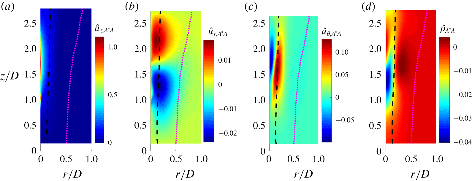
The function  $\hat{\boldsymbol{q}}_{A^{\ast }A}(r,z)$ is given by the following:
 $$\begin{eqnarray}\displaystyle {\mathcal{L}}_{0}\hat{\boldsymbol{q}}_{A^{\ast }A} & = & \displaystyle -{\mathcal{N}}\{\hat{\boldsymbol{q}}_{1m}\}\hat{\boldsymbol{q}}_{1m}^{\ast }-{\mathcal{N}}\{\hat{\boldsymbol{q}}_{1m}^{\ast }\}\hat{\boldsymbol{q}}_{1m}-S_{c}({\mathcal{N}}_{-m}^{s}\{\hat{\boldsymbol{q}}_{1m}\}\hat{\boldsymbol{q}}_{1m}^{\ast }+{\mathcal{N}}_{m}^{s}\{\hat{\boldsymbol{q}}_{1m}^{\ast }\}\hat{\boldsymbol{q}}_{1m})\nonumber\\ \displaystyle & & \displaystyle -\,S_{c}^{2}({\mathcal{N}}_{-m}^{ss}\{\hat{\boldsymbol{q}}_{1m}\}\hat{\boldsymbol{q}}_{1m}^{\ast }+{\mathcal{N}}_{m}^{ss}\{\hat{\boldsymbol{q}}_{1m}^{\ast }\}\hat{\boldsymbol{q}}_{1m}).\end{eqnarray}$$
Note that the source terms on the right of (2.27) are independent of  $\boldsymbol{q}_{o}$, showing that the function
 $\hat{\boldsymbol{q}}_{A^{\ast }A}$ quantifies to leading order in
 $S-S_{c}$, the non-oscillatory, time-averaged distortion that the linear instability imposes on the base flow at
 $S_{c}$. Therefore, we will refer to
 $\hat{\boldsymbol{q}}_{A^{\ast }A}$ as the base-flow distortion function.
The function  $\hat{\boldsymbol{q}}_{AA}(r,z)$ quantifies the spatial distribution of the amplitude associated with the first harmonic of the linear instability and is given by the following:
 $$\begin{eqnarray}(-\text{i}2\unicode[STIX]{x1D714}_{g,m}{\mathcal{B}}+{\mathcal{L}}_{2m})\hat{\boldsymbol{q}}_{AA}=-{\mathcal{N}}\{\hat{\boldsymbol{q}}_{1m}\}\hat{\boldsymbol{q}}_{1m}-S_{c}{\mathcal{N}}_{m}^{s}\{\hat{\boldsymbol{q}}_{1m}\}\hat{\boldsymbol{q}}_{1m}-S_{c}^{2}{\mathcal{N}}_{m}^{ss}\{\hat{\boldsymbol{q}}_{1m}\}\hat{\boldsymbol{q}}_{1m}.\end{eqnarray}$$
At  $O(\unicode[STIX]{x1D716}^{3})$ we obtain,
 $$\begin{eqnarray}\displaystyle \left({\mathcal{B}}\frac{\unicode[STIX]{x2202}}{\unicode[STIX]{x2202}t_{1}}+{\mathcal{L}}\right)\boldsymbol{q}_{3} & = & \displaystyle -{\mathcal{B}}\frac{\unicode[STIX]{x2202}\boldsymbol{q}_{1}}{\unicode[STIX]{x2202}t_{2}}-\unicode[STIX]{x1D6E5}_{s}{\mathcal{B}}_{1}\frac{\unicode[STIX]{x2202}\boldsymbol{q}_{1}}{\unicode[STIX]{x2202}t_{1}}-{\mathcal{N}}\{\boldsymbol{q}_{1}\}\boldsymbol{q}_{2}-{\mathcal{N}}\{\boldsymbol{q}_{2}\}\boldsymbol{q}_{1}\nonumber\\ \displaystyle & & \displaystyle -\,S_{c}\left({\mathcal{N}}^{s}\{\boldsymbol{q}_{1}\}\boldsymbol{q}_{2}+{\mathcal{N}}^{s}\{\boldsymbol{q}_{2}\}\boldsymbol{q}_{1}\right)\nonumber\\ \displaystyle & & \displaystyle -\,S_{c}^{2}\left({\mathcal{N}}^{ss}\{\boldsymbol{q}_{1}\}\boldsymbol{q}_{2}+{\mathcal{N}}^{ss}\{\boldsymbol{q}_{2}\}\boldsymbol{q}_{1}\right)\nonumber\\ \displaystyle & & \displaystyle -\,\unicode[STIX]{x1D6E5}_{s}[{\mathcal{N}}^{s}\{\boldsymbol{q}_{1}\}\boldsymbol{q}_{o}+{\mathcal{N}}^{s}\{\boldsymbol{q}_{o}\}\boldsymbol{q}_{1}+2S_{c}({\mathcal{N}}^{ss}\{\boldsymbol{q}_{1}\}\boldsymbol{q}_{o}+{\mathcal{N}}^{ss}\{\boldsymbol{q}_{o}\}\boldsymbol{q}_{1})-{\mathcal{L}}_{T}^{s}\boldsymbol{q}_{1}].\nonumber\\ \displaystyle & & \displaystyle\end{eqnarray}$$
Physically relevant, non-trivial solutions to (2.29) must be bounded in time and space. As is common, the norm that is used to quantify the magnitude of  $\boldsymbol{q}_{3}$ is generated by the following definition of the inner product between two functions:
 $$\begin{eqnarray}\langle \boldsymbol{q}_{1},\boldsymbol{q}_{2}\rangle =\int _{0}^{Z}\int _{0}^{R}\int _{0}^{2\unicode[STIX]{x03C0}}(\boldsymbol{q}_{1}^{H})^{\text{T}}\boldsymbol{q}_{2}r\,\text{d}\unicode[STIX]{x1D703}\,\text{d}r\,\text{d}z,\end{eqnarray}$$
where the superscript ‘ $H$’ denotes the transpose complex conjugate operation.
Thus, the boundedness condition on  $\boldsymbol{q}_{3}$ requires that the oscillatory contributions with frequency,
 $\unicode[STIX]{x1D714}_{g,m}$, to the source term in (2.29) must be orthogonal to the corresponding adjoint eigenfunction of the operator on the left, associated with the inner product defined in (2.30). These adjoint eigenfunctions can be written as
 $\boldsymbol{q}_{1m}^{\dagger }(r,z,\unicode[STIX]{x1D703},t_{1})=\hat{\boldsymbol{q}}_{1m}^{\dagger }(r,z)\text{e}^{\text{i}(m\unicode[STIX]{x1D703}+\unicode[STIX]{x1D714}_{g,m}^{\dagger }t_{1})}$, where
 $\unicode[STIX]{x1D714}_{g,m}^{\dagger }$ and
 $\hat{\boldsymbol{q}}_{1m}^{\dagger }(r,z)$ are given by solving the following equation:
 $$\begin{eqnarray}(\text{i}\unicode[STIX]{x1D714}_{g,m}^{\dagger }{\mathcal{B}}+{\mathcal{L}}_{m}^{\dagger })\hat{\boldsymbol{q}}_{1m}^{\dagger }=0,\end{eqnarray}$$
where  ${\mathcal{L}}_{m}^{\dagger }$ is the adjoint linear operator that satisfies the following relation,
 $\langle \hat{\boldsymbol{q}}_{1m}^{\dagger },{\mathcal{L}}_{m}\hat{\boldsymbol{q}}_{1m}\rangle =\langle {\mathcal{L}}_{m}^{\dagger }\hat{\boldsymbol{q}}_{1m}^{\dagger },\hat{\boldsymbol{q}}_{1m}\rangle$. This relation, along with (2.19) and (2.31), gives
 $\unicode[STIX]{x1D714}_{g,m}^{\dagger }=\unicode[STIX]{x1D714}_{g,m}^{\ast }$ (see Schmid & Henningson Reference Schmid and Henningson2001).
Thus, substituting (2.18) and (2.25) into (2.29) and invoking the boundedness condition, yields the evolution equation for  $A_{1}(t_{2})$ as follows (Landau & Lifshitz Reference Landau and Lifshitz1959):
 $$\begin{eqnarray}\displaystyle \frac{\text{d}A_{1}}{\text{d}t_{2}}=\unicode[STIX]{x1D6E5}_{s}B_{A}A_{1}-N_{A}A_{1}|A_{1}|^{2}. & & \displaystyle\end{eqnarray}$$
Equation (2.32) is referred to as the Stuart–Landau amplitude evolution equation. The coefficient in the linear term on the right in (2.32),  $B_{A}$, is given by the following inner product:
 $$\begin{eqnarray}\displaystyle B_{A} & = & \displaystyle \frac{1}{\langle \hat{\boldsymbol{q}}_{1m}^{\dagger },{\mathcal{B}}\hat{\boldsymbol{q}}_{1m}\rangle }\langle \!\hat{\boldsymbol{q}}_{1m}^{\dagger },[\!\text{i}\unicode[STIX]{x1D714}_{g,m}{\mathcal{B}}_{1}\hat{\boldsymbol{q}}_{1m}-{\mathcal{N}}\{\hat{\boldsymbol{q}}_{1m}\}\hat{\boldsymbol{q}}_{\unicode[STIX]{x1D6E5}}-{\mathcal{N}}\{\boldsymbol{q}_{\unicode[STIX]{x1D6E5}}\}\hat{\boldsymbol{q}}_{1m}\nonumber\\ \displaystyle & & \displaystyle -\,{\mathcal{N}}_{0}^{s}\{\hat{\boldsymbol{q}}_{1m}\}\boldsymbol{q}_{o}-{\mathcal{N}}_{m}^{s}\{\boldsymbol{q}_{o}\}\hat{\boldsymbol{q}}_{1m}\nonumber\\ \displaystyle & & \displaystyle -\,S_{c} ({\mathcal{N}}_{0}^{s}\{\hat{\boldsymbol{q}}_{1m}\}\hat{\boldsymbol{q}}_{\unicode[STIX]{x1D6E5}}+{\mathcal{N}}_{m}^{s}\{\hat{\boldsymbol{q}}_{\unicode[STIX]{x1D6E5}}\}\hat{\boldsymbol{q}}_{1m}\nonumber\\ \displaystyle & & \displaystyle -\,2{\mathcal{N}}_{0}^{ss}\{\hat{\boldsymbol{q}}_{1m}\}\boldsymbol{q}_{o}-2{\mathcal{N}}_{m}^{ss}\{\boldsymbol{q}_{o}\}\hat{\boldsymbol{q}}_{1m} )\nonumber\\ \displaystyle & & \displaystyle -\,S_{c}^{2}({\mathcal{N}}_{0}^{ss}\{\hat{\boldsymbol{q}}_{1m}\}\hat{\boldsymbol{q}}_{\unicode[STIX]{x1D6E5}}+{\mathcal{N}}_{m}^{ss}\{\hat{\boldsymbol{q}}_{\unicode[STIX]{x1D6E5}}\}\hat{\boldsymbol{q}}_{1m})\nonumber\\ \displaystyle & & \displaystyle +\,{\mathcal{L}}_{T,m}^{s}\hat{\boldsymbol{q}}_{1m}\! ]\!\rangle \!.\end{eqnarray}$$
Thus, it is clear that the growth of flow oscillations, determined by  $B_{A}$ in linear term in (2.32), is in turn determined by
 $\hat{\boldsymbol{q}}_{\unicode[STIX]{x1D6E5}}$, i.e. the intrinsic base-flow modification for
 $S>S_{c}$, which therefore, is the cause of the onset of flow oscillations.
The coefficient of the nonlinear term in (2.32),  $N_{A}$, is given by the following inner product:
 $$\begin{eqnarray}\displaystyle N_{A} & = & \displaystyle \frac{1}{\langle \hat{\boldsymbol{q}}_{1m}^{\dagger },{\mathcal{B}}\hat{\boldsymbol{q}}_{1m}\rangle }\langle \!\hat{\boldsymbol{q}}_{1m}^{\dagger },[\!{\mathcal{N}}\{\hat{\boldsymbol{q}}_{1m}\}\hat{\boldsymbol{q}}_{A^{\ast }A}+{\mathcal{N}}\{\hat{\boldsymbol{q}}_{1m}^{\ast }\}\hat{\boldsymbol{q}}_{AA}\nonumber\\ \displaystyle & & \displaystyle +\,{\mathcal{N}}\{\hat{\boldsymbol{q}}_{A^{\ast }A}\}\hat{\boldsymbol{q}}_{1m}+{\mathcal{N}}\{\hat{\boldsymbol{q}}_{AA}\}\hat{\boldsymbol{q}}_{1m}^{\ast }\nonumber\\ \displaystyle & & \displaystyle +\,S_{c} ({\mathcal{N}}_{0}^{s}\{\hat{\boldsymbol{q}}_{1m}\}\hat{\boldsymbol{q}}_{A^{\ast }A}+{\mathcal{N}}_{2m}^{s}\{\hat{\boldsymbol{q}}_{1m}^{\ast }\}\hat{\boldsymbol{q}}_{AA}\nonumber\\ \displaystyle & & \displaystyle +\,{\mathcal{N}}_{m}^{s}\{\hat{\boldsymbol{q}}_{A^{\ast }A}\}\hat{\boldsymbol{q}}_{1m}+{\mathcal{N}}_{-m}^{s}\{\hat{\boldsymbol{q}}_{AA}\}\hat{\boldsymbol{q}}_{1m}^{\ast })\nonumber\\ \displaystyle & & \displaystyle +\,S_{c}^{2} ({\mathcal{N}}_{0}^{ss}\{\hat{\boldsymbol{q}}_{1m}\}\hat{\boldsymbol{q}}_{A^{\ast }A}+{\mathcal{N}}_{2m}^{ss}\{\hat{\boldsymbol{q}}_{1m}^{\ast }\}\hat{\boldsymbol{q}}_{AA}\nonumber\\ \displaystyle & & \displaystyle +\,{\mathcal{N}}_{m}^{ss}\{\hat{\boldsymbol{q}}_{A^{\ast }A}\}\hat{\boldsymbol{q}}_{1m}+{\mathcal{N}}_{-m}^{ss}\{\hat{\boldsymbol{q}}_{AA}\}\hat{\boldsymbol{q}}_{1m}^{\ast })\!]\!\rangle \!.\end{eqnarray}$$
The expression for  $N_{A}$ in (2.37) can be decomposed into two individual components such that
 $N_{A}=N_{A1}+N_{A2}$. The component,
 $N_{A1}$, is determined by base-flow distortion as follows:
 $$\begin{eqnarray}\displaystyle N_{A1} & = & \displaystyle \frac{1}{\langle \hat{\boldsymbol{q}}_{1m}^{\dagger },{\mathcal{B}}\hat{\boldsymbol{q}}_{1m}\rangle }\langle \!\hat{\boldsymbol{q}}_{1m}^{\dagger },[\!{\mathcal{N}}\{\hat{\boldsymbol{q}}_{1m}\}\hat{\boldsymbol{q}}_{A^{\ast }A}+{\mathcal{N}}\{\hat{\boldsymbol{q}}_{A^{\ast }A}\}\hat{\boldsymbol{q}}_{1m}\nonumber\\ \displaystyle & & \displaystyle +\,S_{c}({\mathcal{N}}_{0}^{s}\{\hat{\boldsymbol{q}}_{1m}\}\hat{\boldsymbol{q}}_{A^{\ast }A}+{\mathcal{N}}_{m}^{s}\{\hat{\boldsymbol{q}}_{A^{\ast }A}\}\hat{\boldsymbol{q}}_{1m})\nonumber\\ \displaystyle & & \displaystyle +\,S_{c}^{2}({\mathcal{N}}_{0}^{ss}\{\hat{\boldsymbol{q}}_{1m}\}\hat{\boldsymbol{q}}_{A^{\ast }A}+{\mathcal{N}}_{m}^{ss}\{\hat{\boldsymbol{q}}_{A^{\ast }A}\}\hat{\boldsymbol{q}}_{1m})\!]\!\rangle \!.\end{eqnarray}$$
The component,  $N_{A2}$, is the component due to harmonic generation as follows:
 $$\begin{eqnarray}\displaystyle N_{A2} & = & \displaystyle \frac{1}{\langle \hat{\boldsymbol{q}}_{1m}^{\dagger },{\mathcal{B}}\hat{\boldsymbol{q}}_{1m}\rangle }\langle \!\hat{\boldsymbol{q}}_{1m}^{\dagger },[\!{\mathcal{N}}\{\hat{\boldsymbol{q}}_{1m}^{\ast }\}\hat{\boldsymbol{q}}_{AA}+{\mathcal{N}}\{\hat{\boldsymbol{q}}_{AA}\}\hat{\boldsymbol{q}}_{1m}^{\ast }\nonumber\\ \displaystyle & & \displaystyle +\,S_{c}({\mathcal{N}}_{2m}^{s}\{\hat{\boldsymbol{q}}_{1m}^{\ast }\}\hat{\boldsymbol{q}}_{AA}+{\mathcal{N}}_{-m}^{s}\{\hat{\boldsymbol{q}}_{AA}\}\hat{\boldsymbol{q}}_{1m}^{\ast })\nonumber\\ \displaystyle & & \displaystyle +\,S_{c}^{2}({\mathcal{N}}_{2m}^{ss}\{\hat{\boldsymbol{q}}_{1m}^{\ast }\}\hat{\boldsymbol{q}}_{AA}+{\mathcal{N}}_{-m}^{ss}\{\hat{\boldsymbol{q}}_{AA}\}\hat{\boldsymbol{q}}_{1m}^{\ast })\!]\!\rangle \!.\end{eqnarray}$$
Next, we rewrite (2.32) in terms of a single time variable,  $t$, by introducing
 $A(t)=\unicode[STIX]{x1D716}A_{1}(\unicode[STIX]{x1D716}^{2}t)+\unicode[STIX]{x1D716}^{2}A_{2}(\unicode[STIX]{x1D716}^{2}t)$ into (2.32), which then yields the following equation at leading order:
 $$\begin{eqnarray}\displaystyle \frac{\text{d}A}{\text{d}t}=(S-S_{c})B_{A}A-N_{A}A|A|^{2}. & & \displaystyle\end{eqnarray}$$
Thus, the asymptotic solution to (2.8), accurate to  $O(\unicode[STIX]{x1D716}^{3})$, is given by
 $$\begin{eqnarray}\displaystyle \tilde{\boldsymbol{q}}(r,z,\unicode[STIX]{x1D703},t) & = & \displaystyle \boldsymbol{q}_{o}(r,z)+(S-S_{c})\hat{\boldsymbol{q}}_{\unicode[STIX]{x1D6E5}}(r,z)+|A(t)|^{2}\hat{\boldsymbol{q}}_{A^{\ast }A}(r,z)\nonumber\\ \displaystyle & & \displaystyle +\,A(t)\hat{\boldsymbol{q}}_{1m}(r,z)\text{e}^{\text{i}m\unicode[STIX]{x1D703}-\text{i}\unicode[STIX]{x1D714}_{g,m}t}+A^{\ast }(t)\hat{\boldsymbol{q}}_{1m}(r,z)^{\ast }\text{e}^{-\text{i}m\unicode[STIX]{x1D703}+\text{i}\unicode[STIX]{x1D714}_{g,m}t}\nonumber\\ \displaystyle & & \displaystyle +\,(A(t))^{2}\hat{\boldsymbol{q}}_{AA}(r,z)\text{e}^{\text{i}2m\unicode[STIX]{x1D703}-\text{i}2\unicode[STIX]{x1D714}_{g,m}t}+(A^{\ast }(t))^{2}\hat{\boldsymbol{q}}_{A^{\ast }A^{\ast }}(r,z)\text{e}^{-\text{i}2m\unicode[STIX]{x1D703}+\text{i}2\unicode[STIX]{x1D714}_{g,m}t}\nonumber\\ \displaystyle & & \displaystyle +\,O((S-S_{c})^{3/2}).\end{eqnarray}$$
Except for the first two terms, the remaining terms in (2.38) are contributions that become relevant when coherent unsteadiness is established in the flow for  $S>S_{c}$. Note that this first happens when the linear hydrodynamic mode,
 $\hat{\boldsymbol{q}}_{1m}$, becomes neutrally stable, i.e.
 $\unicode[STIX]{x1D714}_{g,m}$ is purely real. In this case, the nature of flow unsteadiness for
 $S>S_{c}$ depends on the characteristics of
 $A(t)$. These can be determined by setting
 $A(t)=D(t)\text{e}^{\text{i}\unicode[STIX]{x1D719}(t)}$ in (2.37), where
 $D(t)$ and
 $\unicode[STIX]{x1D719}(t)$ are real-valued functions that represent the time evolution of the amplitude and argument of
 $A(t)$. Thus, equating real parts on both sides of (2.37) yields an evolution equation for
 $D(t)$ as follows:
 $$\begin{eqnarray}\frac{\text{d}D}{\text{d}t}=(S-S_{c})B_{Ar}D-N_{Ar}D^{3},\end{eqnarray}$$
where  $B_{Ar}$ and
 $N_{Ar}$ are the real parts of the coefficients
 $N_{A}$ and
 $B_{A}$, respectively. Thus, the unsteady characteristics of the flow are determined by establishing the behaviour of
 $D(t)$ as
 $t\rightarrow \infty$ for a given non-zero initial perturbation,
 $D_{i}=D(0)$.
Assuming that the flow is nominally stable for  $S<S_{c}$, the following types of unsteady flow behaviour can be identified for
 $S>S_{c}$ based on the signs of
 $B_{Ar}$ and
 $N_{Ar}$ as follows.
(i) Stable limit cycle ( $B_{Ar}>0$,
 $N_{Ar}>0$). For any value of
 $D_{i}>0$, equation (2.39) shows that for
 $S>S_{c}$ the first term causes
 $D(t)$ to increase exponentially, while the second term limits this growth. Eventually,
 $D(t)\rightarrow D_{LC}$ as
 $t\rightarrow \infty$ where
 $D_{LC}$, determined by letting
 $\text{d}D/\text{d}t\rightarrow 0$ in (2.39), is given by
 $$\begin{eqnarray}D_{LC}=\sqrt{\frac{(S-S_{c})B_{Ar}}{N_{Ar}}}.\end{eqnarray}$$
The change in oscillation frequency of the flow from  $\unicode[STIX]{x1D714}_{g,m}$ baseline at
 $S=S_{c}$ with increasing
 $S$ can be determined using (2.39) by choosing
 $A(t)=D_{LC}\text{e}^{\text{i}\unicode[STIX]{x1D714}_{c}t}$ and comparing imaginary parts on both sides to yield:
 $$\begin{eqnarray}\unicode[STIX]{x1D714}_{c}=(S-S_{c})\left[B_{Ai}-B_{Ar}\left(\frac{N_{Ai}}{N_{Ar}}\right)\right].\end{eqnarray}$$
Thus, equation (2.38) shows that the angular frequency,  $\unicode[STIX]{x1D714}_{LC}$, of the limit-cycle oscillation is given by
 $$\begin{eqnarray}\unicode[STIX]{x1D714}_{LC}=\unicode[STIX]{x1D714}_{g,m}-(S-S_{c})B_{Ai}+(S-S_{c})B_{Ar}\left(\frac{N_{Ai}}{N_{Ar}}\right).\end{eqnarray}$$
Note also that for  $S<S_{c}$, both terms on the right of (2.39) cause
 $D(t)\rightarrow 0$ as
 $t\rightarrow \infty$ for any value of
 $D_{i}$. This type of flow behaviour corresponds to a supercritical Hopf bifurcation in the flow state at
 $S=S_{c}$, i.e. the emergence of a stable limit cycle for
 $S>S_{c}$ due to a linear hydrodynamic mode of the system becoming neutrally stable. Thus, the spatial region where the integrand in (2.33) is non-zero can now be identified as the nonlinear wavemaker region, i.e. the region of the flow that contributes to the growth of coherent oscillations. Note that we use the term ‘nonlinear’ to emphasise that this definition of the wavemaker is different from that defined from linear, structural sensitivity considerations (Hill Reference Hill1992; Giannetti & Luchini Reference Giannetti and Luchini2007; Juniper & Pier Reference Juniper and Pier2015; Tammisola & Juniper Reference Tammisola and Juniper2016). Further, we refer to the spatial regions where the integrand in (2.34) is non-zero as the nonlinear wavelimiter region because
 $N_{A}$ determines the impact that the nonlinear terms have in determining the final saturated oscillation amplitude of the limit cycle. Note that (2.34) shows that amplitude saturation is caused by the modification induced on the time-averaged flow for
 $S>S_{c}$ as well as interaction between the linear eigenmode and its first harmonic.
(ii) Subcritical flow ( $B_{Ar}>0$,
 $N_{Ar}<0$). In this case, equation (2.39) suggests that for
 $S>S_{c}$,
 $D(t)\rightarrow \infty$ as
 $t\rightarrow \infty$ for any value of
 $D_{i}$. This suggests that
 $S=S_{c}$ represents a catastrophic loss of stability. As such, the flow dynamics cannot be quantitatively described by the present leading-order nonlinear analysis. On the other hand, for
 $S<S_{c}$, an unstable limit cycle with an amplitude
 $D_{LC}=\sqrt{(S-S_{c})B_{Ar}/N_{Ar}}$ exists. Note that for
 $D_{i}<D_{LC}$,
 $\text{d}D/\text{d}t<0$ and therefore,
 $D(t)\rightarrow 0$ as
 $t\rightarrow \infty$. For
 $D_{i}>D_{LC}\,\text{d}D/\text{d}t>0$ and therefore,
 $D(t)\rightarrow \infty$ as
 $t\rightarrow \infty$. Thus, coherent flow unsteadiness is triggered when
 $D>D_{LC}$ for
 $S<S_{c}$.
(iii) Stable flow ( $B_{Ar}\leqslant 0$,
 $N_{Ar}>0$). For this case, equation (2.39) shows that
 $D(t)\rightarrow 0$ as
 $t\rightarrow \infty$ for any value of
 $D_{i}$.
Note that other possibilities for  $N_{Ar}$ and
 $B_{Ar}$ are not considered as they do not result in steady flow behaviour for
 $S<S_{c}$. We next use these results to gain insight into the emergence of globally self-excited helical oscillations in a variable swirl jet experiment that will be described in the next section.
3 Experimental study
Experiments were conducted in a swirling flow facility with the ability to continually vary the swirl number of the jet. The main components of the set-up, shown in figure 1, relevant to the analysis performed in this work are: the injector nozzle, the swirler chamber with a variable-angle, radial-entry swirler and the settling chamber. Room temperature air enters the settling chamber via the air inlet port at the bottom of the rig. Upstream of this inlet, the air passes through a flow meter (Teledyne Hastings) with a 0.5 % flow rate uncertainty. In all cases tested, the flow rate remained with 0.12 % of the  $19.0~\text{g}~\text{s}^{-1}$ set point that corresponds to a bulk flow velocity (
 $U_{o}$) of
 $36~\text{m}~\text{s}^{-1}$.
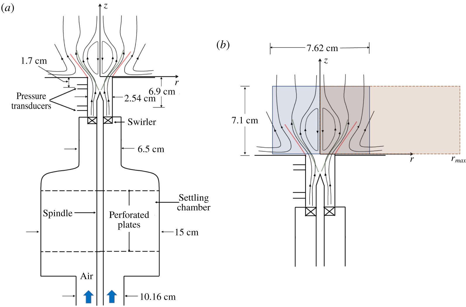
Schematic of experimental set-up. The blue box downstream of the dump plane shows the field of view of the sPIV measurements. The red box shows schematically the computational domain. The streamlines are shown for purpose of illustration alone. The nominal Reynolds number based on jet nozzle diameter,  $Re=59\,000$.

Air enters the settling chamber through a flow-conditioning section comprised of perforated plates at each end to breakup large turbulent structures. A smooth contraction downstream reduces the diameter of the duct from 15 to 6.5 cm in order to create a radially uniform velocity distribution upstream of the radial-entry swirler block. The flow enters the variable-angle swirler radially and exits to the atmosphere through a 2.54 cm diameter nozzle. The nozzle is fitted with two pressure transducers, as shown in figure 1. The pressure transducers (PT) are located 6.92 cm and 1.7 cm from the nozzle exit. PCB Piezotronics model 113B28 pressure transducers are used. The pressure transducer signal is amplified using PCB Piezotronics four channel, ICP sensor signal conditioner, model 482C26. The pressure signal is recorded using LabView through a National Instruments DAQ at 20 kHz for a duration of three seconds.
The variable-angle, radial-entry swirler allows for the swirl number to be changed continuously without changing the net mass flow rate of air entering the set-up. The swirler consists of eight evenly spaced movable vanes with a NACA 0025 airfoil cross-section. The span and chordwise dimensions of each vane are both 2.54 cm. The angle of the blades relative to the radius of the duct can be changed using an encoded stepper motor within the range of  $-70^{\circ }$ to
 $70^{\circ }$.
A Hawk/Darwin Duo Nd-YAG, 532 nm wavelength, 60 W laser is used for measuring three components of velocity using stereoscopic particle image velocimetry in the  $r{-}z$ plane. The blue rectangle in figure 1 shows schematically the laser sheet and the field of view used to acquire raw images using two Photron SA5 complementary metal oxide semiconductor high-speed cameras. The sampling rate of the PIV system is 5 kHz, with an interframe time ranging from 22 to
 $24~\unicode[STIX]{x03BC}\text{s}$ depending on swirl number. Images are recorded for a one-second duration, yielding 5000 frames of velocity field data per test case.
Aluminium oxide particles with a nominal diameter of  $0.5{-}2~\unicode[STIX]{x03BC}\text{m}$ are used as tracer particles and can accurately follow flow perturbations up to a frequency of 4000 Hz. Velocity vectors are calculated in DaVis 8.3.1 without any preprocessing or masking and stereoscopic cross-correlation with multi-pass iterations and with decreasing window sizes. The first pass is a
 $32\times 32$ pixel interrogation window with a 50 % overlap followed by two passes with a
 $16\times 16$ pixel interrogation with a 50 % overlap. During vector post processing, there are two methods used to reject vectors. First, if the vector is more than three times the root mean square of the surrounding vectors, the vector is removed and replaced. Additionally, universal outlier detection removes and replaces spurious vector results. The uncertainty was calculated on the mean vector field for each test case and did not exceeded
 $2~\text{m}~\text{s}^{-1}$.
4 Flow field characterization
This section discusses the evolution of the flow field characteristics of the swirling jet as determined from sPIV measurements. We define a geometric swirl number,  $S$, in this paper to quantify the intensity of swirl as follows:
 $$\begin{eqnarray}S=\frac{2}{3}\tan \unicode[STIX]{x1D6FC}\left[\frac{1-(R_{c}/R_{b})^{3}}{1-(R_{c}/R_{b})^{2}}\right],\end{eqnarray}$$
where  $\unicode[STIX]{x1D6FC}$ is the swirler vane angle,
 $R_{c}$ is the centrebody radius and
 $R_{b}$ is the swirler tube radius (see figure 1). The expression in (4.1) can be derived from the momentum flux based definition of swirl number (Beér & Chigier Reference Beér and Chigier1972) by assuming an axial inflow into an annulus with inner and outer radii,
 $R_{c}$ and
 $R_{b}$, respectively, undergoing a deflection through and angle
 $\unicode[STIX]{x1D6FC}$ as it passes through the swirl vanes. At each swirl number, the flow is defined by a certain state; pre-vortex breakdown, near-vortex breakdown, steady vortex breakdown, weak PVC and strong PVC (Clees et al. Reference Clees, Lewalle, Frederick and O’Connor2018). Pre-vortex breakdown swirling jets correspond to
 $0\leqslant S\leqslant 0.38$, before a central recirculation zone forms. The near-vortex breakdown state occurs when
 $0.38<S\leqslant 0.67$ and is characterized by highly intermittent recirculation along the jet centreline. The steady vortex breakdown state occurs beyond this range of
 $S$ wherein a stable central recirculation zone is established around the centreline of the jet. We begin our discussion of these flow characteristics by first examining the time-averaged characteristics of the flow field with increasing
 $S$.
4.1 Time-averaged characteristics
Variation of the time-averaged axial velocity field with  $S$ (
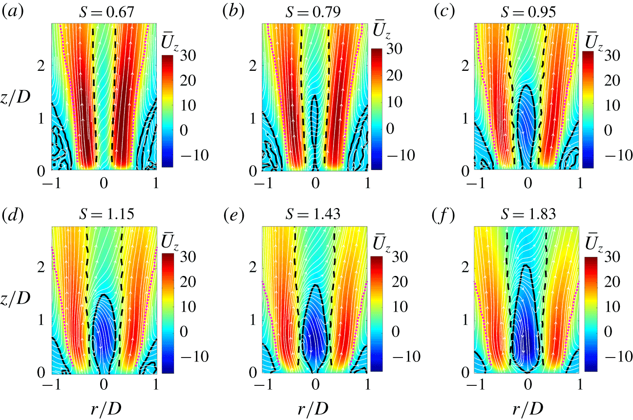
 $Re=59\,000$) with streamlines. The solid black curve shows the time-averaged recirculation zone. The broken curves show the nominal location of the inner (black) and outer (magenta) shear layers in the time-averaged flow.

The evolution of the time-averaged flow field for  $S=0.67{-}1.83$ is shown in figure 2. In each of the figures, the colour field shows
 $\bar{U}_{z}$. Streamlines in white are overlaid to visualize the direction of the flow. The broken black and magenta lines denote the time-averaged location of the shear layers in the flow. These curves are determined from the radial position of the inflection points in the
 $\bar{U}_{z}$ profile at each
 $z$ location. The thick black contours correspond to
 $\bar{U}_{z}=0$ and denote the boundaries of the recirculation zones. The same scheme is used to label these time-averaged flow field features in all field plots in the rest of this paper.
Figure 2 shows that increasing  $S$ leads to increased jet spreading due to the formation of the breakdown bubble, whose boundaries are captured by the thick black
 $\bar{U}_{z}=0$ contour. Note that the absence of a bubble for the
 $S=0.67$ case is due to the fact that for this case, the bubble is still intermittent and hence does not appear in the time-averaged result presented in figure 2(a). This change in the time-averaged flow field structure is accompanied by the emergence of a coherent flow oscillation in the jet. We next present results that characterize the nature of the flow oscillation in the next subsection.
4.2 Unsteady dynamics
We characterize the global spatial structure of flow oscillations using the spectral proper orthogonal decomposition (SPOD) on the time-resolved flow field measurements from sPIV. The SPOD calculates the optimal energy-ordered but spectrally resolved basis modes that can be used to reconstruct the unsteady flow field (Towne, Schmidt & Colonius Reference Towne, Schmidt and Colonius2018). Thus, SPOD is a superior method for identifying narrowband oscillations when compared to the traditional proper orthogonal decomposition (POD), which does not discern modes based on frequency. As such, highly tonal but low-energy oscillations that are not necessarily separated from other unsteady motions by the POD are unambiguously identified by the SPOD. All results from SPOD in this paper have been determined by dividing the time record of sPIV measurements into 18 ensembles with 256 points per ensemble and 50 % overlap between successive ensembles for the spectral estimation step.
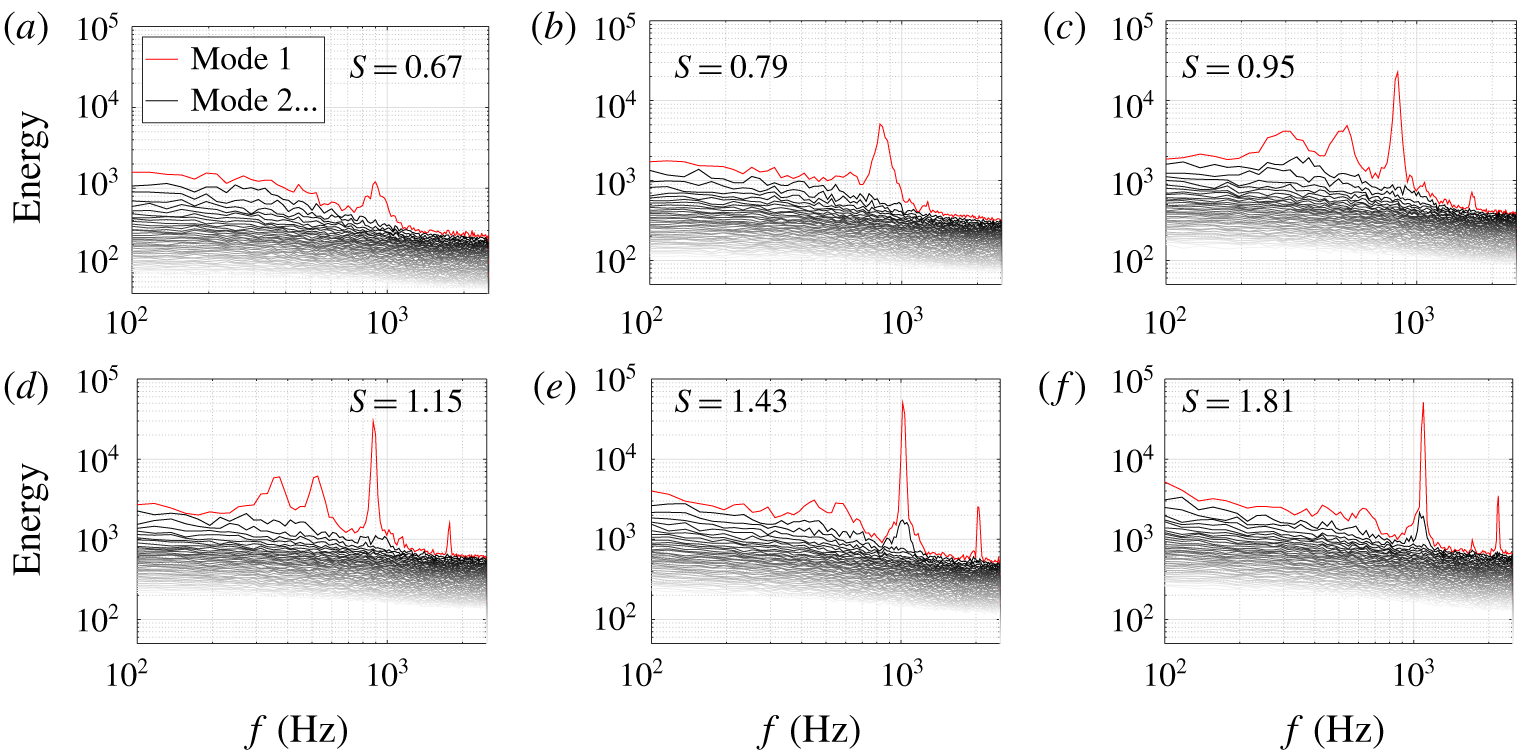
Figure 3(a–e) shows the mode energy spectra from SPOD for  $S=0.67{-}1.83$. The mode energy spectra show the energy spectra for each mode, where mode 1, the most energetic mode, is highlighted in red and the remainder of the modes fade from black to grey in descending order of total mode energy. As
 $S$ is increased, the peak frequency, which appears in mode 1 between 800 and 1100 Hz for each case, increases as well. Additionally, the energy of the mode increases in amplitude and decreases in spectral width as the coherence of the PVC increases. At the highest two swirl numbers shown,
 $S=1.43$ and 1.83, some of the PVC energy appears in the second mode (mode 2) as well, where a smaller, more broadband peak is present beneath the mode 1 spectrum. Additionally, the first harmonic of the PVC appears in mode 1 at the higher swirl number cases, a result of the very high amplitude coherent oscillation.
Another feature that appears in mode 1 of the SPOD for swirl numbers in the range  $S=0.95{-}1.15$ (see figure 3c,d) is two additional peaks near 500 Hz and 300 Hz. A continuous wavelet transform analysis of the velocity fluctuations at several points in the annular jet near the nozzle exit for these two values of
 $S$ showed that these peaks are due to an intermittent turbulent burst that occurred at frequencies of 300 Hz and 500 Hz. Further, the pressure transducer signals show no evidence of these oscillations (Manoharan Reference Manoharan2019). Note, however, that the energy associated with these fluctuations is an order of magnitude less than that associated with the coherent oscillation. As such, they are not the focus of the discussion in this paper.
Variation of the energy spectra with  $S$ from spectral proper orthogonal decomposition of the time-resolved flow fields determined from sPIV measurements (
 $Re=59\,000$). The red curve shows the spectrum for the most energetic mode. The spectra for the remaining modes are shown in grey scale from high (dark) to low (light) total energy. The values of
 $S$ associated with each result are shown within each plot.

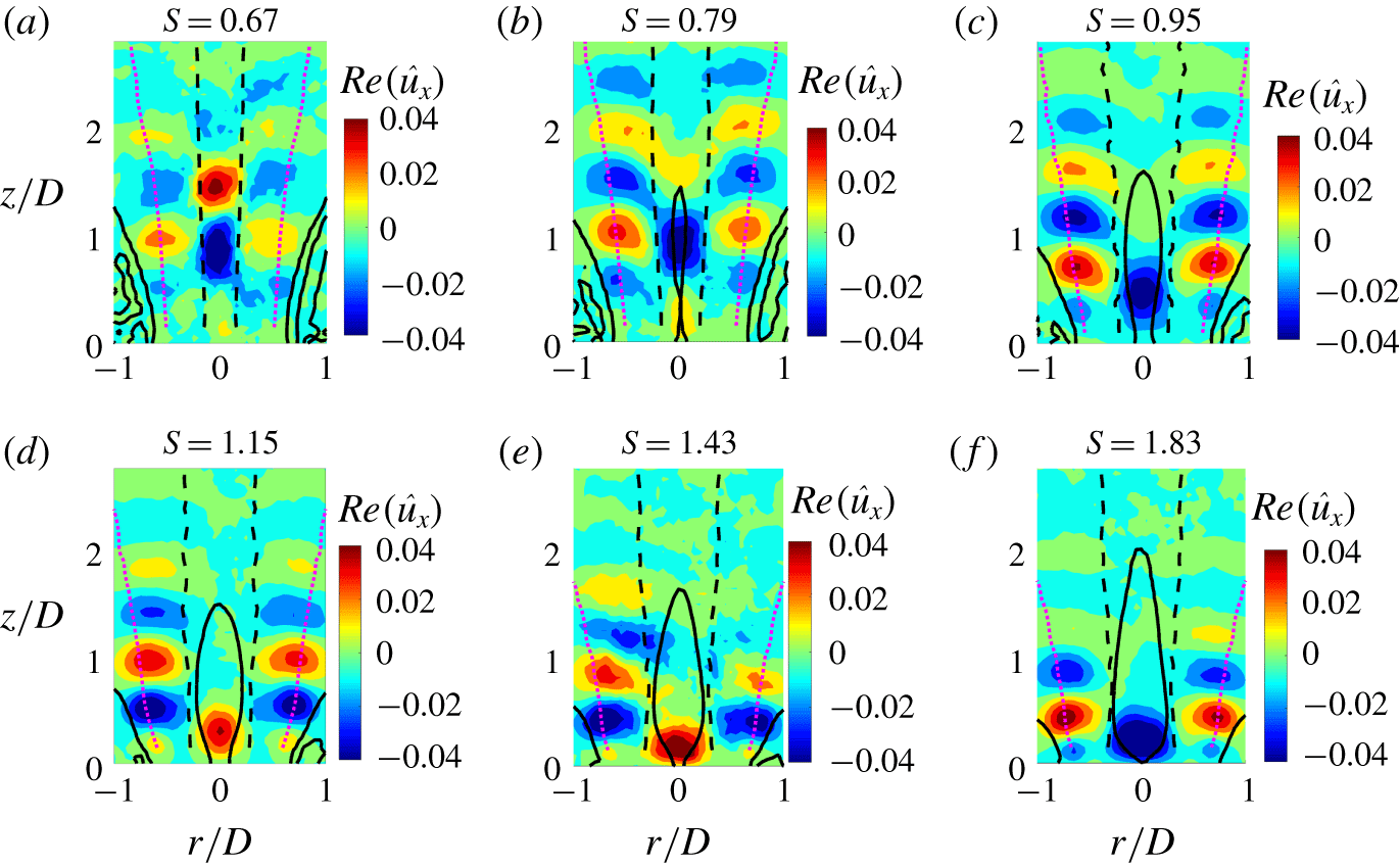
Variation of the horizontal in plane velocity component modes determined from spectral proper orthogonal decomposition at the PVC frequency,  $f_{PVC}$, with
 $S$ (
 $Re=59\,000$). The value of
 $S$ associated with each result is shown on the title of each of the plots. The solid black curve shows the time-averaged recirculation zone boundary. The broken curves show the nominal location of the inner (black) and outer (magenta) shear layers in the time-averaged flow.

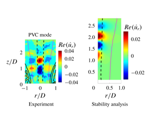
Figure 4(a–f) shows the normalized mode shapes corresponding to the mode 1 peak frequency at each value of  $S$. Each figure shows the real part of the horizontal velocity component in the plane of light sheet,
 $Re(\hat{u} _{x})$, associated with each SPOD mode. These mode shapes show the evolution of the spatial dynamics of the coherent oscillation as a function of
 $S$. Note first that the mode at
 $S=0.67$ shows a mode shape with strong oscillations on the centreline, which suggests that the coherent oscillation induces a precession of the axial vortex. Therefore, we identify the coherent oscillation associated with the frequency corresponding to the peak in figure 3(a–e) as the precessing vortex core (Syred Reference Syred2006). We will show in a forthcoming section of this paper that the PVC is a consequence of the formation of the breakdown bubble in the flow, using the results from the theoretical analysis presented in § 2. It is useful at this point to emphasize the distinction between the PVC oscillations shown in figure 4 and helical spiral breakdown studied by Meliga et al. (Reference Meliga, Gallaire and Chomaz2012) and Qadri et al. (Reference Qadri, Mistry and Juniper2013). In these two studies, the helical rollup of the shear layers is due to the instability of helical modes that have significant oscillation amplitudes downstream of the breakdown bubble. The PVC oscillation on the other hand is associated with the precession of the vortex breakdown bubble and results in shear layer rollup that originates at the upstream end of the breakdown bubble as figure 4 and other prior experimental studies show (Escudier & Keller Reference Escudier and Keller1985; Oberleithner et al. Reference Oberleithner, Sieber, Nayeri, Paschereit, Petz, Hege, Noack and Wygnanski2011).
With increasing  $S$, figure 4(a–e) shows that the centreline oscillation moves upstream into the nozzle. This is consistent with the prior observation of Escudier & Keller (Reference Escudier and Keller1985) in a very similar experimental set-up. Also, the region where the centreline oscillations are concentrated lies at the upstream end of the bubble, consistent with observations in prior studies with experimental set-ups similar to ours (Escudier & Keller Reference Escudier and Keller1985; Escudier Reference Escudier1988; Oberleithner et al. Reference Oberleithner, Sieber, Nayeri, Paschereit, Petz, Hege, Noack and Wygnanski2011). Note also that the oscillations along the OSL become progressively stronger relative to those on the centreline with increasing
 $S$ due to the development of helical oscillations of the shear layers in the flow downstream of the bubble.
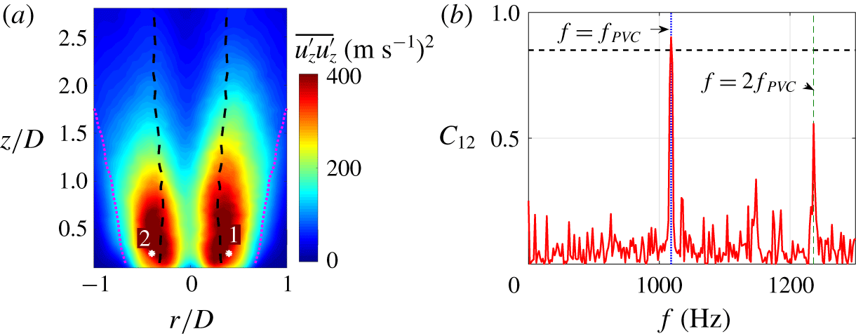
We next estimate the azimuthal mode number associated with the PVC oscillation and the critical swirl number,  $S_{c}$, at which it emerges from a spatial cross-spectral analysis of the sPIV results as follows. Figure 5(a) shows the spatial variation of
 $\overline{u_{z}^{\prime }u_{z}^{\prime }}$ determined from the sPIV measurements at
 $S=1.83$. The broken black and magenta curves show the nominal position of the ISL and the OSL respectively. Points 1 and 2, positioned at (
 $r/D=\pm 0.4$,
 $z/D=0.25$) (see figure 5a), are chosen as reference points for cross-spectral analysis (Bendat & Piersol Reference Bendat and Piersol2011). All cross-spectrum values are computed by dividing the time record of signals at points 1 and 2 into 19 ensembles with 500 samples each and with 50 % overlap between successive ensembles. Figure 5(b) shows a typical result for the variation of the magnitude of the cross-spectrum,
 $|C_{12}|$, between
 $u_{z}^{\prime }$ signals at these two points (
 $S=1.83$). Note that
 $|C_{12}|$ shows a strong peak (
 ${\sim}0.9$) at 1090 Hz, which is close to the value of the peak frequency in the corresponding SPOD spectra for mode 1 – see figure 3(e) – as may be expected. In the rest of this paper, we define the characteristic PVC oscillation frequency (
 $f_{PVC}$) as the frequency at which the maximum value of
 $|C_{12}|$ occurs.
Variation of (a)  $\overline{u_{z}^{\prime }u_{z}^{\prime }}$ in
 $r{-}z$ plane. (b) Coherence (
 $|C_{12}|$) as a function of frequency for
 $S=1.83$. The broken curves show the nominal location of the inner (black) and outer (magenta) shear layers in the time-averaged flow for this case.

Figure 5(b) also shows a second peak at the first harmonic,  $f_{1h}=2f_{PVC}$, consistently with the corresponding spectrum from the SPOD (figure 4e). The lower value of
 $|C_{12}|\sim 0.6$ at
 $f_{1h}$ (see figure 5b) is because of smaller amplitudes of velocity oscillation at
 $f_{1h}$ and therefore, lower signal-to-noise ratio when compared with
 $f_{PVC}$. These results are typical and similar results are observed at other spatial locations for this case and for other cases with
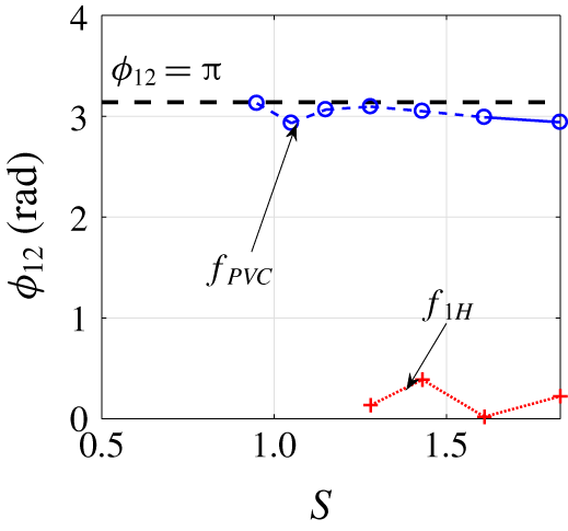
 $S\geqslant 0.67$. The Fourier mode number,
 $m$, associated with the oscillations at
 $f_{PVC}$ and
 $f_{1h}$, can be determined from the phase,
 $\unicode[STIX]{x1D719}_{12}$, of
 $C_{12}$ at these frequencies for each
 $S$. Figure 6(a) shows the variation
 $\unicode[STIX]{x1D719}_{12}$ with
 $S$, determined at
 $f_{PVC}$ and
 $f_{1h}$. The data in figure 6 correspond to values of
 $S$ at which
 $|C_{12}|\geqslant 0.7$ at
 $f_{PVC}$ and
 $|C_{12}|\geqslant 0.5$ at
 $f_{1h}$. Note that
 $\unicode[STIX]{x1D719}_{12}\sim \unicode[STIX]{x03C0}$ for all
 $S$, suggesting that the PVC oscillation shown in figure 4 corresponds to
 $m=1$ helical oscillations, as may be expected. The corresponding result for
 $f_{1h}$ shows that
 $\unicode[STIX]{x1D719}_{12}\sim 0$, which suggests that the first harmonic corresponds to an
 $m=2$ oscillation. These results are typical and, although not shown here, similar variations for
 $\unicode[STIX]{x1D719}_{12}$ with
 $S$ are observed at other downstream locations as well. Also, note that this difference in
 $m$ values associated with the PVC and its first harmonic is consistent with the general asymptotic solution for stable limit-cycle oscillations determined from the theoretical analysis, equation (2.38).
Variation of the phase of the cross-spectrum between axial velocity signals at points 1 and 2, ( $\unicode[STIX]{x1D719}_{12}$) at
 $f_{PVC}$ and
 $f_{1h}=2f_{PVC}$, with
 $S$ (
 $Re=59\,000$).

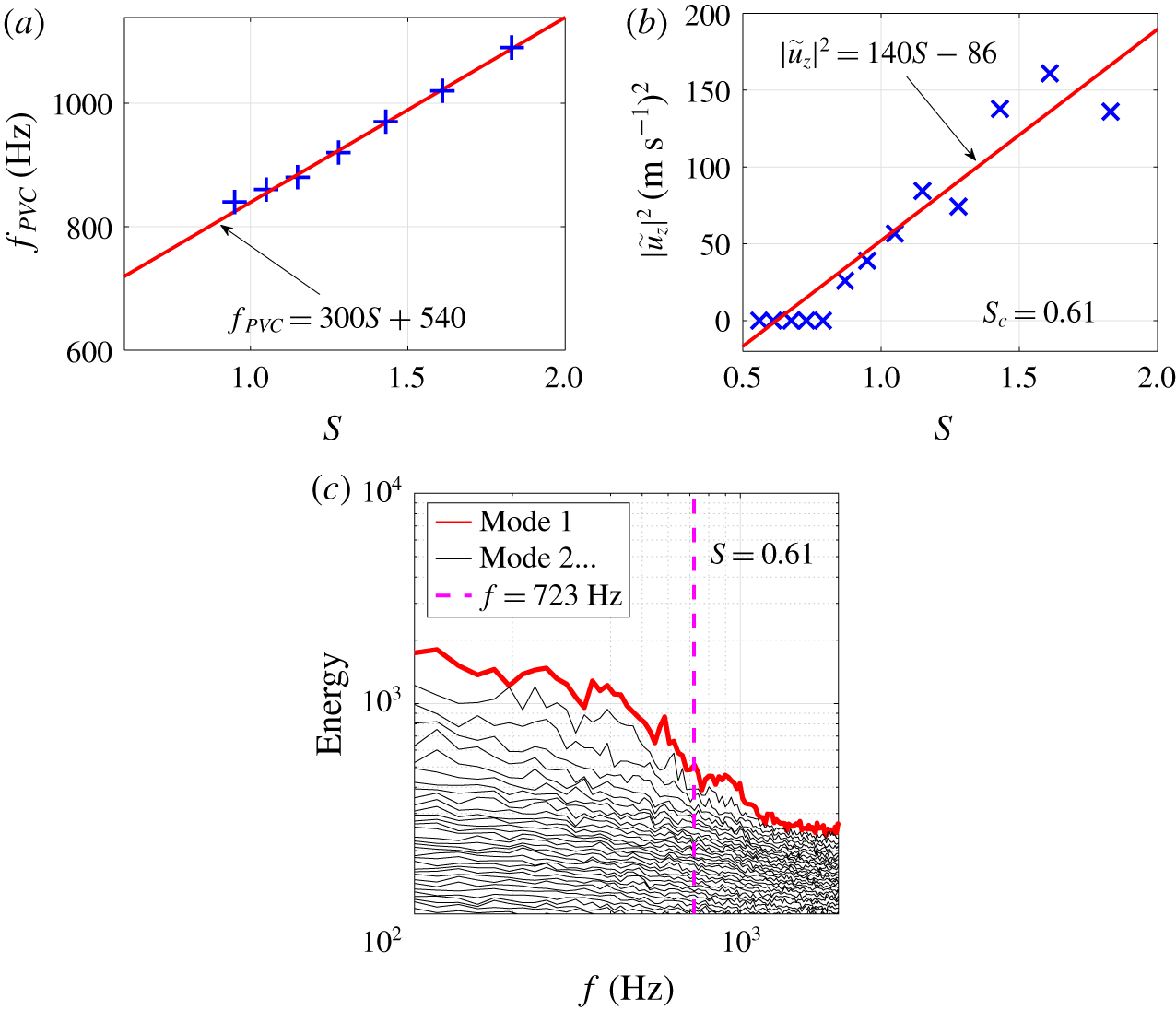
Variation of (a)  $f_{PVC}$ and (b)
 $|\hat{u} _{z}|^{2}$ as a function of
 $S$. The solid lines show linear fits through the experimental values. Panel (c) shows the SPOD spectrum for the
 $S=0.61$ case. The broken vertical line corresponds to
 $f=723~\text{Hz}$, determined from the fit in (a).

We next determine the critical swirl number,  $S_{c}$, at which the coherent PVC oscillation emerges as follows. Figures 7(a) and 7(b) show the variation of
 $f_{PVC}$ and
 $|u_{z}^{\prime }|^{2}$ at
 $f_{PVC}$, respectively, with
 $S$. The data in figure 7(b) have been determined from the component at
 $f_{PVC}$, of the continuous wavelet transform,
 $\tilde{u} _{z}$, of the velocity time series at point 1 (see figure 5a). All non-zero data shown in figure 7(a,b) correspond to values of
 $S$ for which
 $|C_{12}|\geqslant 0.7$ at their respective
 $f_{PVC}$ values. Linear least-squares fits through the data, determined using non-zero values for
 $f_{PVC}$ and
 $|u_{z}^{\prime }|^{2}$, have been superposed in each case. The upstream movement of the breakdown bubble can induce changes to
 $|u_{z}^{\prime }|^{2}$ at point 1 because its distance from the region where the PVC oscillation amplitude is maximum, varies as the bubble moves upstream with increasing
 $S$. However, figure 7(a,b) qualitatively show a nearly linear variation of
 $f_{PVC}$ and
 $|u_{z}^{\prime }|^{2}$ with
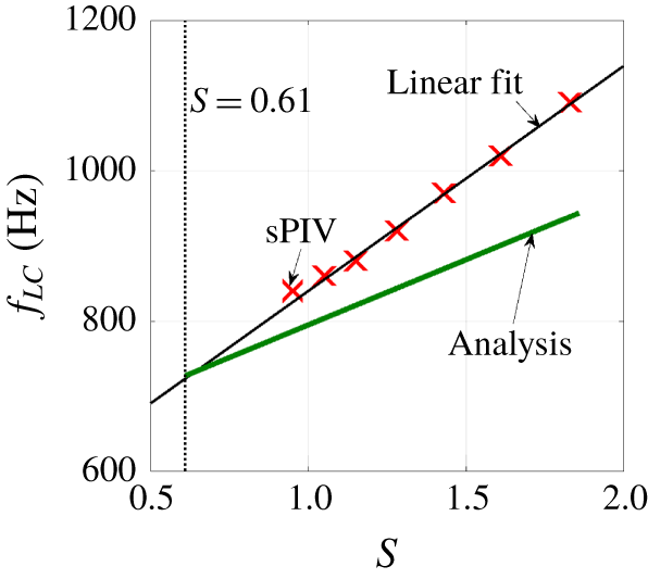
 $S$. This is consistent with the results in (2.40) and (2.42) and hence suggest that the jet undergoes a supercritical Hopf bifurcation. Requiring
 $|\tilde{u} _{z}|^{2}=0$ at
 $S=S_{c}$ yields, from the linear fits shown in figure 7(a,b),
 $S_{c}\sim 0.61$ and
 $f_{PVC}=723~\text{Hz}$ at
 $S_{c}$. Figure 7 shows the spectrum determined from SPOD of the sPIV measured velocity fields at
 $S=0.61$. The broken vertical line in figure 7 corresponds to
 $f=723~\text{Hz}$. Note that this result shows no evidence of a coherent oscillation when compared with the results in figure 3. This result, together with those in figure 3, additionally confirms that the bifurcation in the flow state does indeed occur at
 $S=0.61$.
It is interesting to note here that Oberleithner et al. (Reference Oberleithner, Sieber, Nayeri, Paschereit, Petz, Hege, Noack and Wygnanski2011) report additional evidence for the occurrence of supercritical Hopf bifurcation from experiments wherein the PVC is axially forced near the jet exit using an arrangement of loudspeakers. Their results show that the forcing amplitude needed to synchronize the oscillation frequency of the PVC with that of the forcing scales linearly with  $|\,f-f_{PVC}|$, where
 $f$ is the forcing frequency. These results suggest that the underlying PVC oscillation is a stable limit cycle and is therefore produced by a supercritical Hopf bifurcation process, at least in the present class of variable swirl jet experiments.
We confirm the above facts in this paper by determining a series of results from the weakly nonlinear theory presented in § 2. The time-averaged base-flow field,  $\boldsymbol{q}_{o}$, at
 $S=S_{c}$, needed to compute these results is determined from sPIV measurements at
 $S=0.61$. Further, we adopt a numerical approach to solve the various equations presented in § 2. All of these details are discussed in the next section.
5 Numerical methods
For all computations performed in this paper, the reference length,  $l_{ref}$, and reference axial velocity,
 $\bar{U}_{z,ref}$, are chosen as the jet exit diameter (2.54 cm) and the bulk flow velocity (
 $U_{o}=36~\text{m}~\text{s}^{-1}$). The reference azimuthal velocity component,
 $\bar{U}_{\unicode[STIX]{x1D703},ref}$, is then chosen as
 $0.61U_{o}$ at the critical swirl number of
 $S=0.61$. The physical extents of the flow domain captured in the present computations correspond to the rectangular region lying between
 $0<r<r_{max}$, as shown in figure 1. The physical
 $r{-}z$ space is mapped into the computational space,
 $(\unicode[STIX]{x1D709},\unicode[STIX]{x1D702})\in [-1,1]\times [-1,1]$, using a modified form of the mapping functions given by Bayliss, Class & Matkowsky (Reference Bayliss, Class and Matkowsky1995) (see appendix C). The parameter
 $r_{max}$ represents the maximum radial extent of the solution domain at which far-field boundary conditions, equation (2.23), are imposed. Our numerical tests revealed that choosing values of
 $r_{max}$ between 10 and 50 was adequate to ensure the convergence of solutions for all cases computed in this paper. Accordingly, we set
 $r_{max}=50$ for all computational results presented in this paper. The extents of the domain in the axial direction and are chosen to be
 $z_{min}=0.15$ and
 $z_{max}=2.8$, i.e.
 $0.15D$ from the jet exit plane to the downstream extent of the flow region over which flow field measurements from sPIV are available. At the upstream boundary we assume that velocity perturbations vanish, i.e.
 $$\begin{eqnarray}\hat{u} _{r}=\hat{u} _{\unicode[STIX]{x1D703}}=\hat{u} _{z}=0.\end{eqnarray}$$
At the downstream boundary ( $z=z_{max}$) we impose the following Neumann boundary condition:
 $$\begin{eqnarray}\frac{\unicode[STIX]{x2202}\hat{u} _{r}}{\unicode[STIX]{x2202}z}=\frac{\unicode[STIX]{x2202}\hat{u} _{\unicode[STIX]{x1D703}}}{\unicode[STIX]{x2202}z}=\frac{\unicode[STIX]{x2202}\hat{u} _{z}}{\unicode[STIX]{x2202}z}=0.\end{eqnarray}$$
Note that the boundary conditions in (5.1) and (5.2) are artificial and are needed because of having to choose a finite axial extent for the computational domain imposed by the field of view of the sPIV measurements in this direction. Consequently, their use in this paper is justified only for those cases for which the spatial extent of the region where  $\hat{\boldsymbol{q}}_{1m,d}$ is non-zero is sufficiently far away from these boundaries.
5.1 Linear and leading-order nonlinear solutions
The global linear stability problem given by (2.19), along with (2.20)–(2.22) and (5.1)–(5.2), are solved using the pseudospectral collocation method (Boyd Reference Boyd2000). Accordingly, all dependent variables are written in terms of Chebyshev polynomials of the second kind using function values defined on a two-dimensional mesh of Gauss–Lobatto points in computational space. The parameters in (C 1) and (C 2) are tuned to ensure sufficient collocation point density in physical space in the regions where shear layers of the time-averaged flow field are located and at the domain centreline. The radial and the axial derivatives in (2.19) are replaced by equivalent discrete differentiation matrices (Boyd Reference Boyd2000), which yields a generalized matrix eigenvalue problem as follows:
 $$\begin{eqnarray}A\hat{\boldsymbol{q}}_{1m,d}=\text{i}\unicode[STIX]{x1D714}_{g,m}B\hat{\boldsymbol{q}}_{1m,d},\end{eqnarray}$$
where  $B$ and
 $A$ are matrices representing the discrete equivalent of continuous operators
 ${\mathcal{B}}$ and
 ${\mathcal{L}}_{m}$, respectively. Also,
 $\unicode[STIX]{x1D714}_{g,m}$ is the complex eigenvalue and
 $\hat{\boldsymbol{q}}_{1m,d}$ the discrete equivalent of the eigenfunction
 $\hat{\boldsymbol{q}}_{1m}$ in (2.19). The boundary conditions are written in discrete form and are imposed by replacing the rows corresponding to points on the boundaries in
 $B$ and
 $A$. The eigenvalue problem given in (5.3) is solved using the Arnoldi iterative solver ‘eigs’ available in MATLAB.
The solutions for the adjoint mode are obtained using the discrete adjoint approach outlined in Juniper & Pier (Reference Juniper and Pier2015) as follows. First, the inner product, equation (2.30), is discretized using Gauss–Chebyshev quadrature in computational space as  $\langle \hat{\boldsymbol{q}}_{1,d},\hat{\boldsymbol{q}}_{2,d}\rangle =\hat{\boldsymbol{q}}_{1,d}^{H}M\hat{\boldsymbol{q}}_{2,d}$, where
 $M$ is the matrix generated by the weights of the quadrature rule and the superscript ‘
 $H$’ denotes the transpose conjugate. The matrices of the discrete adjoint problem corresponding to (5.3) are now given by
 $A^{\dagger }=M^{-1}A^{H}M$ and
 $B^{\dagger }=M^{-1}B^{H}M$. Thus, the adjoint mode,
 $\hat{\boldsymbol{q}}_{1m,d}^{\dagger }$, is computed using the ‘eigs’ iterative solver as well.
Variation of  $E=|\unicode[STIX]{x1D714}_{g,-1}^{k+1}-\unicode[STIX]{x1D714}_{g,-1}^{k}|$ as a function of number of collocation points using the swirling base flow from computations reported in Pradeep (Reference Pradeep2018) of the
 $Re=200$ and
 $S=1$ case discussed in Meliga et al. (Reference Meliga, Gallaire and Chomaz2012). The superscript
 $k$ indexes computations in increasing order of
 $N_{I}$.

We validate our linear stability analysis solver against the results reported by Meliga et al. (Reference Meliga, Gallaire and Chomaz2012) for the most unstable  $m=-1$ mode of an unconfined swirling jet undergoing a spiral-type vortex breakdown at
 $S=1.0$ and
 $Re=200$. The base flow for the validation case is obtained from flow simulations performed by Pradeep (Reference Pradeep2018). These simulations are performed on a on a cuboidal computational domain that extends 15 jet inflow diameters in the streamwise direction and 20 jet inflow diameters in the transverse direction. The domain was discretized using 481 and 241 points in the streamwise and transverse directions respectively. These solutions were obtained using the INCOMPACT3D solver (Laizet & Li Reference Laizet and Li2011). The solution captures unsteady flow features described by Meliga et al. (Reference Meliga, Gallaire and Chomaz2012) for this case (see Pradeep (Reference Pradeep2018) for details).
Linear stability computations are performed on a computational mesh comprising  $N$ points each in the radial and axial directions in the computational domain. The quasi-steady flow solutions are interpolated onto the linear stability computational mesh at each axial location using cubic spline interpolation along the radial direction. Figure 8 shows the variation of
 $E=|\unicode[STIX]{x1D714}_{g,-1}^{k+1}-\unicode[STIX]{x1D714}_{g,-1}^{k}|$ with the number of collocation points in the streamwise direction (
 $N_{I}$). Note that the vertical axis uses a logarithmic scale. The superscript
 $k$ indexes the computation in the order of increasing
 $N_{I}$. The value
 $\unicode[STIX]{x1D714}_{g,-1}$ is the prediction from our numerical solutions. Note that
 $E\sim 1\times 10^{-4}$ for
 $N_{I}=120$. The curve fit through the data, shown in figure 8, shows that
 $\unicode[STIX]{x1D714}_{g,-1}^{k}$ converges exponentially with grid refinement, as can be expected for the present pseudospectral method. Table 1 shows the values of
 $\unicode[STIX]{x1D714}_{g,-1}$ for
 $N_{I}=120$ and the final converged value reported by Meliga et al. (Reference Meliga, Gallaire and Chomaz2012). The value of
 $N_{DOF}$ in table 1 refers to the total number of degrees of freedom for three-dimensional state vector in each study. The small difference between these results (
 ${\sim}2.5\,\%$) validates the implementation of the linear global stability solver used in the present study.
Most unstable  $m=-1$ mode eigenvalues for the
 $Re=200$,
 $S=1.0$ case reported in Meliga et al. (Reference Meliga, Gallaire and Chomaz2012). Present results are determined using the swirling base flow from computations reported in Pradeep (Reference Pradeep2018). The value of
 $N_{DOF}$ refers to the total number of degrees of freedom for three-dimensional state vector.

Once the linear stability solutions have been determined, the leading-order nonlinear solutions are determined from (2.28)–(2.26). These are solved by replacing spatial derivatives occurring in the operators on the left with the discrete differentiation matrices and solving the resulting linear system using LU decomposition. The Stuart–Landau coefficients are then determined using (2.34) and (2.33), using the discretized inner product.
We apply the numerical methods described in this section to the time-averaged base-flow state at  $S=0.61$ as determined from sPIV measurements in order to gain insight into the fundamental physical mechanism that results in the emergence of PVC oscillations. Note that the fact that the optimal locations for collocation points do not correspond to the centres of the interrogation windows used while processing the sPIV measurements. Accordingly, the base-flow state on the computational mesh is determined using a combination of interpolation and extrapolation procedures as will be described next.
5.2 Base flow
Figure 9(a–c) shows the spatial variation of the time-averaged velocity components,  $\bar{U}_{z}$,
 $\bar{U}_{\unicode[STIX]{x1D703}}$ and
 $\bar{U}_{r}$ determined using sPIV at
 $S=0.61$. Three-point moving-average filtering of these time-averaged fields is used to remove small length scale oscillations due to uncertainties in the experimental data. The spatial variations of
 $\bar{U}_{z}$ and
 $\bar{U}_{\unicode[STIX]{x1D703}}$ (figure 9a,b) show expected symmetry characteristics across the flow centreline. However, the spatial variation of
 $\bar{U}_{r}$ (figure 9c) is not perfectly anti-symmetric about
 $r=0$, as one may expect. This is because the presence of turbulence in the flow along with intermittent vortex breakdown observed for this case, both of which cause the rotational axis of the flow to ‘wobble’ incoherently about the geometric jet centreline; details of this process are described in Clees et al. (Reference Clees, Lewalle, Frederick and O’Connor2018). Ideally, given a long enough time record, one can expect that the impact of these incoherent flow centreline oscillations would average out, yielding an axisymmetric
 $\bar{U}_{r}$ field (Syred, O’Doherty & Froud Reference Syred, O’Doherty and Froud1994). However, the fact that figure 9(c) shows that this is not the case suggests that the intensity of turbulence fluctuations in the present experiment is comparable to
 $\bar{U}_{r}$ and that additional flow field samples are necessary to achieve good statistical confidence in the data. We next describe how base-flow velocity fields for stability analysis computations are determined from these sPIV measurements.
Time-averaged velocity fields (a)  $\bar{U}_{z}$ (b)
 $\bar{U}_{\unicode[STIX]{x1D703}}$ (c)
 $\bar{U}_{r}$ (
 $S=0.61$,
 $Re=59\,000$). The broken curves show the nominal location of the inner (black) and outer (magenta) shear layers in the time-averaged flow.

Note that the collocation points used for computations do not necessarily lie at the same locations in physical space as the interrogation window centres used in sPIV processing. Also, the field of view of the cameras used in the experiments limits the availability of sPIV data to a region corresponding to  $0\leqslant r<1.5$ around the geometric centreline of the flow. Therefore, we use a combination of interpolation and extrapolation using sPIV data to determine base flow
 $\bar{U}_{\unicode[STIX]{x1D703}}$ and
 $\bar{U}_{z}$ fields for
 $1.5<r\leqslant 50$ as follows. First, least-squares fits to the time-averaged
 $\bar{U}_{\unicode[STIX]{x1D703}}$ and
 $\bar{U}_{z}$ sPIV data of model flow profiles for a swirling jet are determined using the model flow profiles for a swirling jet suggested by Oberleithner et al. (Reference Oberleithner, Sieber, Nayeri, Paschereit, Petz, Hege, Noack and Wygnanski2011). Next, individual cubic spline fits to the radial profiles of
 $\bar{U}_{\unicode[STIX]{x1D703}}$ and
 $\bar{U}_{z}$ at each
 $z$ are determined. A uniform interpolation is then constructed by smoothly merging the cubic spline fits with the fits to model flow profiles at each
 $z$ in a small region centred at
 $r=1.5$ using a hyperbolic tangent function. Figure 10(a,b) shows typical radial profiles of
 $\bar{U}_{\unicode[STIX]{x1D703}}$ and
 $\bar{U}_{z}$ at
 $z=1$ determined from the fitting procedure. The time-averaged sPIV data are overlaid on these profiles for comparison. These results are typical and a similar quality of agreement with sPIV data is seen at other
 $z$ locations as well. The values of
 $\bar{U}_{\unicode[STIX]{x1D703}}$ and
 $\bar{U}_{z}$ at the collocation points on the computational mesh are determined using these fits.
Extrapolated time-averaged velocity fields at  $z/D=1$ (a)
 $\bar{U}_{z}$ (b)
 $\bar{U}_{\unicode[STIX]{x1D703}}$ (
 $S=0.61$,
 $Re=59\,000$).

We determine the  $\bar{U}_{r}$ field from the measured
 $\bar{U}_{z}$ field using the fact that the time-averaged flow must be divergence free rather than use the experimentally measured result shown in figure 9(c). This ensures that our stability analysis is anchored around a base flow that satisfies the time-averaged mass balance condition. This constraint on the time-averaged flow field yields,
 $$\begin{eqnarray}\left(\frac{\unicode[STIX]{x2202}}{\unicode[STIX]{x2202}r}+\frac{1}{r}\right)\bar{U}_{r}=-\frac{\unicode[STIX]{x2202}\bar{U}_{z}}{\unicode[STIX]{x2202}z},\end{eqnarray}$$
along with  $\bar{U}_{r}=0$ at
 $r=0$ (centreline). The spatial derivatives in (5.4) are discretized using the same Chebyshev pseudospectral scheme described in the previous subsection. The resulting linear system of equations for
 $\bar{U}_{r}=0$ at the collocation points in the domain is solved using an LU decomposition. Figure 11 shows the
 $\bar{U}_{r}$ field computed thus. For all computations involving
 $\bar{U}_{r}$, the field shown in figure 11 is used instead of the corresponding time-averaged sPIV field (see figure 9c).
Next, the turbulent viscosity,  $\unicode[STIX]{x1D708}_{T}$, field is determined as follows. Reynolds stress components in the region
 $0<r\leqslant 1.5$ are determined on the sPIV mesh from the sPIV measurements. These values are then interpolated onto the computational mesh using the same interpolation procedure as was used for the time-averaged velocity. The value of each of the Reynolds stresses is allowed to smoothly vanish for
 $r\geqslant 1.5$ using a hyperbolic tangent function. The
 $\unicode[STIX]{x1D708}_{T}$ field is then determined using (B 3) at each point. Figure 12 shows the spatial variation of
 $\unicode[STIX]{x1D708}_{T}$ normalized by the value of the molecular viscosity,
 $\unicode[STIX]{x1D708}$. As may be expected,
 $\unicode[STIX]{x1D708}_{T}$ is concentrated between the two shear layers and increases with axial distance downstream. Note that (B 3) represents the solution to an unconstrained least-squares minimization problem. Also, the experimental uncertainty in the measured velocity values, translate into uncertainty in the Reynolds stresses and mean strain-rate fields. Both of these reasons cause
 $\unicode[STIX]{x1D708}_{T}$ to become negative in some regions of the flow. We find that these values appear predominantly in regions where turbulence intensities are small. Accordingly, we set to
 $\unicode[STIX]{x1D708}_{T}=0$ at all points where
 $\unicode[STIX]{x1D708}_{T}<0$ in order to avoid the generation of spurious eigenvalues in the linear stability analysis (Rukes et al. Reference Rukes, Paschereit and Oberleithner2016).
Base-flow field for  $\bar{U}_{r}$ determined from time-averaged sPIV profiles for
 $\bar{U}_{\unicode[STIX]{x1D703}}$ and
 $\bar{U}_{z}$ using the divergence free constraint (
 $S=0.61$,
 $Re=59\,000$). The broken curves show the nominal location of the inner (black) and outer (magenta) shear layers in the time-averaged flow.

Turbulent viscosity,  $\unicode[STIX]{x1D708}_{T}$, field determined from sPIV data at
 $S_{c}=0.61$ (
 $Re=59\,000$). The broken curves show the nominal location of the inner (black) and outer (magenta) shear layers in the time-averaged flow.

All curve fitting and linear equation solutions discussed in this subsection is performed using functions available as part of MATLAB. The results presented in this paper use meshes that have between 60 and 65 points in the axial direction and 80 and 100 points in the radial direction. These limits represent the finest meshes possible such that there are no more than two collocation points per cell of the sPIV data. For all cases, the number and location of collocation points in physical space were refined until the change in the magnitude of all physically relevant eigenvalues was less than  $1\times 10^{-5}$ between successive grid refinements.
6 Results
We present results from the analysis described in § 2, which show that the flow undergoes vortex breakdown at  $S_{c}=0.61$, resulting in the formation of an axisymmetric breakdown bubble. The PVC oscillation shown in figures 3 and 4 is due to the emergence of a linearly marginally stable hydrodynamic mode that results in the formation of a stable limit cycle. We first discuss the the formation of a recirculation zone on the jet centreline with increasing
 $S$.
6.1 Vortex breakdown
Figure 13(a–d) shows the spatial variation of the four components that comprise the intrinsic base-flow modification,  $\hat{\boldsymbol{q}}_{\unicode[STIX]{x1D6E5}}$, given by (2.26). The broken black and magenta curves in each of the plots in figure 13(a–c) show the nominal locations of the time-averaged inner and outer shear layers. It is clear that
 $\hat{u} _{z,\unicode[STIX]{x1D6E5}}$ (figure 13a) imposes an axial reverse flow near the jet centreline on the baseline time-averaged flow field at
 $S=0.61$ (see figure 9), resulting in an outward radial deflection of the oncoming flow as
 $\hat{u} _{r,\unicode[STIX]{x1D6E5}}$ (figure 13b) shows.
Spatial variation of velocity components of  $\hat{q}_{\unicode[STIX]{x1D6E5}}$ (a)
 $\hat{u} _{z,\unicode[STIX]{x1D6E5}}$ (b)
 $\hat{u} _{r,\unicode[STIX]{x1D6E5}}$ (c)
 $\hat{u} _{\unicode[STIX]{x1D703},\unicode[STIX]{x1D6E5}}$ and (d)
 $\hat{p}_{\unicode[STIX]{x1D6E5}}$ (
 $S=0.61$,
 $Re=59\,000$). The broken curves show the nominal location of the inner (black) and outer (magenta) shear layers in the time-averaged flow.

The reason for this reverse flow in the axial direction is due to the development of a streamwise adverse hydrodynamic pressure gradient within the jet, as figure 13(d) shows. This adverse pressure gradient develops due to pressure recovery along the axial direction resulting from a decrease in  $\bar{U}_{\unicode[STIX]{x1D703}}$ caused by the loss of confinement as the jet exits the nozzle (see figure 9b). As such, the present results suggest that the inception of vortex breakdown for swirling jets exiting a nozzle into, generally speaking, a ‘less-confined’ region is simply due to the formation of an adverse axial pressure gradient. Mathematically, the present analysis supports this conclusion as (2.26) shows that the intrinsic base flow changes, quantified by
 $\hat{\boldsymbol{q}}_{\unicode[STIX]{x1D6E5}}$, depend only on the details of the base flow at
 $S=S_{c}$. Also, equation (2.38) shows that the quantitative impact of the fields shown in figure 13 increases with increasing
 $S$. Thus, the axial pressure gradient induced by
 $\hat{p}_{\unicode[STIX]{x1D6E5}}$ (see figure 13d) increases with increasing
 $S$ causing the flow stagnation point to move upstream.
Several theories have been proposed in the past for explaining the onset of vortex breakdown in swirling flows based on the analogy with boundary layer separation, hydrodynamic instability and the existence of long wavelength spatially oscillatory standing wave disturbances (see Benjamin Reference Benjamin1962; Hall Reference Hall1972; Leibovich Reference Leibovich1978). For cases where the solutions to (2.26) have similar characteristics as shown in figure 13, the theory of Benjamin (Reference Benjamin1962) appears to be the most plausible explanation for the onset of axisymmetric breakdown. A recent analysis evaluating the outcomes of this theory in the context of laminar swirling flows can be found in Moise & Mathew (Reference Moise and Mathew2019).
Note that (2.33) shows that the coefficient  $B_{A}$, which, from (2.32), can potentially result in the growth of flow oscillations for
 $S>S_{c}$, depends only on
 $\hat{\boldsymbol{q}}_{\unicode[STIX]{x1D6E5}}$ and
 $\hat{\boldsymbol{q}}_{1m}$. This means that the PVC flow oscillations in the present experiment are caused by the formation of the axisymmetric breakdown bubble. Thus, in general, the analysis presented in § 2 suggests that the various types of unsteady breakdown states observed in swirling flows (Sarpkaya Reference Sarpkaya1971a,Reference Sarpkayab; Liang & Maxworthy Reference Liang and Maxworthy2005) correspond to the emergence of hydrodynamic instabilities associated with the mean flow state after axisymmetric vortex breakdown has occurred. The nature of the final unsteady state depends on the specific hydrodynamic modes whose instability causes the bifurcation in the flow state.
Global eigenvalue spectrum for  $S=0.61$ (
 $m=1$,
 $Re=59\,000$). (a) Spectrum computed for nominal
 $\unicode[STIX]{x1D708}_{T}$, (b) sensitivity of spectrum to the value of
 $\unicode[STIX]{x1D708}_{T}$. The vertical broken lines in both figures mark the value of
 $\unicode[STIX]{x1D714}_{PVC}$ as determined from the linear fit to the experimental data shown in figure 7(a).

6.2 Stability analysis
Prior local parallel flow linear stability analyses on time-averaged base-flow profiles performed by the present author and others show that for sufficiently high values of  $S$, reverse flow on the centreline can cause the emergence of locally absolutely unstable helical (i.e.
 $m=1$) modes (Olendraru & Sellier Reference Olendraru and Sellier2002; Gallaire & Chomaz Reference Gallaire and Chomaz2003a,Reference Gallaire and Chomazb; Oberleithner et al. Reference Oberleithner, Sieber, Nayeri, Paschereit, Petz, Hege, Noack and Wygnanski2011, Reference Oberleithner, Stöhr, Im, Arndt and Steinberg2015; Manoharan et al. Reference Manoharan, Hansford, OConnor and Hemchandra2015, Reference Manoharan, Smith, Emerson, Douglas, Lieuwen and Hemchandra2017; Frederick et al. Reference Frederick, Manoharan, Dudash, Brubaker, Hemchandra and O’Connor2018; Manoharan Reference Manoharan2019). Local absolute instability can result in global linear hydrodynamic modes that are marginally stable (Chomaz et al. Reference Chomaz, Huerre and Redekopp1991; Monkewitz et al. Reference Monkewitz, Huerre and Chomaz1993). We show that this is indeed the case for the present experiment from the global hydrodynamic stability analysis at
 $S_{c}=0.61$.
Figure 14(a) shows the global eigenvalue spectrum for  $m=1$ (helical) oscillations at
 $S=0.61$ that the global linear stability analysis yields. The vertical line at
 $\unicode[STIX]{x1D714}_{g,r}\sim 3.2$ corresponds to the angular frequency associated with
 $f_{PVC}=723~\text{Hz}$ at
 $S_{c}=0.61$, as determined from the linear fit to experimentally determined values of
 $f_{PVC}$ – see figure 7(a) and accompanying discussion. As may be expected, figure 14 shows that there is an isolated marginally stable eigenmode with
 $\unicode[STIX]{x1D714}_{g}=3.2+\text{i}(-0.25)$, which we designate as ‘GM1’ in this paper. Stability analysis for other
 $m$ values did not yield eigenmodes with similar oscillation frequencies for the
 $S_{c}=0.61$ case. Also, SPOD spectra at
 $S=0.61$, determined from experiments, did not show the presence of coherent oscillations. Therefore, we conclude that GM1 is the helical (
 $m=1$) eigenmode that determines the characteristics of the bifurcation in the flow state at
 $S_{c}=0.61$ and the resulting unsteady coherent flow oscillation characteristics for
 $S>S_{c}$.
We now discuss possible reasons for the global stability of GM1 ( $\unicode[STIX]{x1D714}_{g,i}\sim -0.25$). This may be attributed primarily to quantitative uncertainty in the
 $\unicode[STIX]{x1D708}_{T}$ field. We assess the sensitivity of
 $\unicode[STIX]{x1D714}_{g}$ to
 $\unicode[STIX]{x1D708}_{T}$ by re-computing linear eigenvalue spectra by applying a spatially uniform scale factor on the baseline
 $\unicode[STIX]{x1D708}_{T}$ field shown in figure 12. Figure 14(b) shows spectra for the baseline case (crosses),
 $0.5\unicode[STIX]{x1D708}_{T}$ (circles) and
 $0.25\unicode[STIX]{x1D708}_{T}$ (filled boxes). The arrows in figure 14(b) label the eigenvalue corresponding to GM1. It is clear that the sensitivity of
 $\unicode[STIX]{x1D714}_{g,i}$ to
 $\unicode[STIX]{x1D708}_{T}$ is much more significant than that of
 $\unicode[STIX]{x1D714}_{g,r}$ and that the mode tends towards neutral stability as
 $\unicode[STIX]{x1D708}_{T}$ is reduced. This suggests that the baseline
 $\unicode[STIX]{x1D708}_{T}$ determined from the sPIV measurements (see figure 12) is possibly larger than what it should be for the present jet. Also,
 $S_{c}=0.61$ is the last experimental condition in the present sPIV measurements for which no coherent flow oscillations are observed in the SPOD spectra. This suggests that the exact value of
 $S_{c}$ may be slightly greater than 0.61, which, in addition to the uncertainty in
 $\unicode[STIX]{x1D708}_{T}$, results in the linear stability analysis predicting a stable GM1 mode.
Spatial variation eigenvector components of the mode GM1 (real part only shown) (a)  $\hat{u} _{r}$ (b)
 $\hat{u} _{\unicode[STIX]{x1D703}}$ (c)
 $\hat{u} _{z}$ (
 $S=0.61$,
 $Re=59\,000$). The broken curves show the nominal location of the inner (black) and outer (magenta) shear layers in the time-averaged flow.

Figure 15(a–c) shows the spatial variation of the oscillation amplitude (real part) of the various velocity components comprising the eigenvector,  $\hat{\boldsymbol{q}}_{1m}$, associated with GM1. Figure 15(a–c) shows that this mode induces strong oscillations at the geometric centreline of the flow. Further, equation (2.38) shows that, to leading order in
 $(S-S_{c})$, the spatial amplitude distribution of this mode determines the spatial amplitude distribution of the flow oscillation at the PVC frequency. Thus, it is reasonable to compare the linear mode amplitude distribution with the result from the SPOD analysis at
 $S=0.67$, i.e. for the first experimental condition after the bifurcation in the flow state. Comparing figure 4(a) with the result in figure 15(a), shows that the centreline oscillations occur over the same axial extent in both the linear stability result in figure 15(a–c) and the experimentally determined SPOD mode for
 $S=0.67$ (figure 4a). The wavelength of these oscillations is similar in both results as well. These results further confirm that the emergence of PVC oscillations is due to the emergence of a linearly marginally stable mode at
 $S_{c}=0.61$ in the present swirling jet experiment.
However, the eigenvector solutions shown in figure 15 do not show finite amplitude oscillations in the outer shear layer as observed in the SPOD modes (figure 4). This may be attributed to the large values of  $\unicode[STIX]{x1D708}_{T}$ in this region, as figure 12 shows. Further, with increasing
 $S$, the increase in centreline backflow velocity results in an increase in the strength of the shear layer between the breakdown bubble and the surrounding flow. This then results in a spatially growing response to flow perturbations imposed on the time-averaged flow by GM1, thereby, causing shear layer rollup. Note from figure 4 that the shear layer oscillations appear to originate from the leading end of the breakdown bubble where the centreline oscillations generated by GM1 are strongest. Also, the amplitude of shear layer oscillations increases with increasing
 $S$. These trends suggest that shear layer oscillations are a response to perturbations imposed by the PVC. We note here that a similar hypothesis for shear layer oscillations has been suggested by Oberleithner et al. (Reference Oberleithner, Sieber, Nayeri, Paschereit, Petz, Hege, Noack and Wygnanski2011), based on the similarity between the spatial structure of flow oscillations determined from weakly non-parallel linear hydrodynamic stability analysis at the PVC frequency and POD modes determined from PIV measurements, in their variable swirl jet experiment.
Spatial distribution of magnitudes of the integrands that determine the linear growth and saturation of the flow oscillation amplitude (a)  $I_{BA}$ (b)
 $I_{NA1}$ (c)
 $I_{NA2}$ (
 $S=0.61$,
 $Re=59\,000$).

We next compute the Stuart–Landau constants  $N_{A}$ and
 $B_{A}$ using (2.34) and (2.33), respectively, in order to determine the nature of the bifurcation in the flow state at
 $S=S_{c}$ due to GM1. It is interesting to examine the spatial distribution of the integrands that comprise the inner products in (2.33), (2.35) and (2.36), denoted as
 $I_{BA}$,
 $I_{NA1}$ and
 $I_{NA2}$, respectively. Figure 16 show the spatial variation of the magnitude of each of these quantities in the flow domain. Note also, that figure 16(a) shows that the primary contribution to
 $B_{A}$ is from the region just upstream of where the amplitudes associated with GM1 are significant. This is easily seen by comparing the results in figure 15 with those in figure 16(a). As discussed in § 2 – see discussion below (2.42) – the region where
 $|I_{BA}|$ is large (see figure 16a) is the nonlinear wavemaker region for the PVC at
 $S=S_{c}$. Interestingly, the location of the wavemaker is at the upstream end of the breakdown region for the PVC, which is consistent with the prediction from linear structural sensitivity considerations (Tammisola & Juniper Reference Tammisola and Juniper2016).
Variation of  $f_{LC}$ as a function of
 $S$ obtained from weakly nonlinear analysis. The ‘
 $\times$’ markers show the corresponding variation of
 $f_{PVC}$ determined from sPIV data. A linear fit through the data is shown for reference (thin line). The vertical dotted line is at the critical swirl number,
 $S_{c}=0.61$.

Thus, the values of  $B_{A}$ and
 $N_{A}$ determined from (2.33) and (2.34) are as follows:
 $$\begin{eqnarray}B_{A}=1.5+\text{i}(1.6)\quad N_{A}=0.56+\text{i}(0.9).\end{eqnarray}$$
Note that the results in figure 16(a–c) confirm that the present computational domain captures all non-zero contributions to the integrands in the inner products of (2.33), (2.35) and (2.36), and that the axial domain length limitation imposed by the axial extents of the field of view in the sPIV measurements does not quantitatively affect the value of  $N_{A}$ and
 $B_{A}$. Thus, the values of in (6.1) (
 $B_{Ar}>0$ and
 $N_{Ar}>0$) confirm that a supercritical Hopf bifurcation in the flow state occurs at
 $S_{c}=0.61$ and that the PVC oscillation in the flow is due to the emergence of a stable limit cycle as discussed in § 2 – see (2.40).
Figure 17 compares predictions for the limit-cycle frequency,  $f_{LC}$, determined from (2.42) using the values of
 $N_{A}$ and
 $B_{A}$ given in (6.1). Note that the present stability analysis (solid line) predicts an increasing
 $f_{LC}$ with
 $S$ with a slightly different slope that of the experiment. The difference in the slopes between the two results can be attributed to two reasons. The first and primary reason is the quantitative uncertainty in the
 $\unicode[STIX]{x1D708}_{T}$ field discussed earlier. These directly influence
 $B_{A}$ and
 $N_{A}$ through the last term in (2.33) and
 $\hat{\boldsymbol{q}}_{AA}$ – see (2.28) and (2.34). The second reason is that the value of
 $S_{c}=0.61$ used in the present analysis is the largest value of
 $S$ in the current experimental dataset for which no coherent mode was observed in the SPOD spectra. Thus, it is possible that in reality
 $0.61<S_{c}<0.67$ where
 $S=0.67$ is the first condition for
 $S>0.61$ at which sPIV measurements are available. Thus, it is possible that using linear stability results at
 $S=0.61$ introduces errors in the value of
 $B_{A}$ and
 $N_{A}$, leading to a difference in the predicted slop from the experiment. Nevertheless, the result in figure 17 represents the best possible match between experiment and analysis that is possible with the present sPIV dataset and together with the fact that the harmonic of
 $f_{PVC}$ corresponds to an oscillation with
 $m=2$, (see figure 6), as the present theory suggests, confirm that the PVC is indeed a stable limit-cycle oscillation caused by the emergence of an axisymmetric vortex breakdown bubble in the jet.
Spatial variation of the components of  $\hat{q}_{A^{\ast }A}$, (a)
 $\hat{u} _{z,A^{\ast }A}$ (b)
 $\hat{u} _{r,A^{\ast }A}$ (c)
 $\hat{u} _{\unicode[STIX]{x1D703},A^{\ast }A}$ and (d)
 $\hat{p}_{A^{\ast }A}$ (
 $S=0.61$,
 $Re=59\,000$). The broken curves show the nominal location of the inner (black) and outer (magenta) shear layers in the time-averaged flow.

We next examine the impact that the PVC oscillation induced by GM1 has on the time-averaged base-flow field. Note that this impact is quantified by  $\hat{\boldsymbol{q}}_{A^{\ast }A}$ – see (2.38). Further, from (2.38), it is clear that the influence of
 $\hat{\boldsymbol{q}}_{A^{\ast }A}$ scales linearly with
 $S-S_{c}$ to leading order. Figure 18(a–d) shows the spatial variation of
 $\hat{u} _{z,A^{\ast }A}$,
 $\hat{u} _{r,A^{\ast }A}$,
 $\hat{u} _{\unicode[STIX]{x1D703},A^{\ast }A}$ and
 $\hat{p}_{z,A^{\ast }A}$ components of
 $\hat{\boldsymbol{q}}_{A^{\ast }A}$. The broken black and magenta lines show the nominal location of the inner and outer axial shear layers in the time-averaged flow for the
 $S_{c}=0.61$ case for reference.
Figure 18(d) shows that the axial vortex core precession induced by GM1 creates a pocket of low hydrodynamic pressure near the flow centreline over the axial extent where the flow oscillations due to GM1 are significant – compare figures 18(d) and 15(b). This pocket of low pressure induces a radially inward deflection of the flow as figure 18(b) shows. Eventually, the flow must turn at the centreline resulting in a strong axial velocity being induced in the direction of the overall flow as figure 18(a) shows. The helical nature of the flow oscillations also has an impact on  $\bar{U}_{\unicode[STIX]{x1D703}}$ as shown by the spatial variation of
 $\hat{u} _{\unicode[STIX]{x1D703},A^{\ast }A}$ in figure 18(c). Thus, with increasing
 $S>S_{c}$ it is clear from (2.38) that
 $\hat{\boldsymbol{q}}_{A^{\ast }A}$ counteracts the impact of
 $\hat{\boldsymbol{q}}_{\unicode[STIX]{x1D6E5}}$, resulting in a shortening of the length of the breakdown bubble and an overall reduction in the centreline reverse flow velocity magnitude. Figure 16(b,c) shows that the nonlinear wavelimiter region, i.e. the flow region contributing to nonlinear amplitude saturation of the PVC (see discussion below (2.42)), is located downstream of the nonlinear wavemaker. This may be expected as the impact of
 $\hat{\boldsymbol{q}}_{A^{\ast }A}$ becomes more significant with increasing distance downstream of the nonlinear wavemaker as figure 18(a–d) suggests.
We next discuss insights that can be gained from the asymptotic solution in (2.38) on the general question of the usefulness of linear stability analysis in understanding the coherent unsteady behaviour of turbulent flow fields, given an estimate of their time-averaged flow state. In a practical engineering design scenario, it is not always easy to determine the value of  $S_{c}$ for a given nozzle geometry. Therefore, it is interesting to know whether linear stability analysis can be used to predict coherent unsteady behaviour of turbulent swirled flows, in general for
 $S>S_{c}$, using only the time-averaged flow field as an input. For this discussion, it is useful to view (2.38) as the leading-order estimate of the exact solution for the unsteady coherent component of the flow at any general value of
 $S$. Thus, the mathematical structure of (2.38) suggests the following points:
(i) The first three terms in (2.38) represent the time-averaged flow field at a general value of
 $S$.
(ii) For unsteady coherent flow oscillations resulting from the emergence of a stable limit-cycle flow state (i.e. a supercritical Hopf bifurcation), the mathematical form of the first oscillatory term in (2.38) suggests that a linear stability analysis using the time-averaged flow at any
$S>S_{c}$ should yield a nearly neutral mode at the limit-cycle frequency given by $\unicode[STIX]{x1D714}_{LC}$.


Sipp & Lebedev (Reference Sipp and Lebedev2007) discuss the validity of the second point above in their study of flow state bifurcations in two-dimensional laminar flows using a weakly nonlinear analysis with the bifurcation parameter as  $Re^{-1}$. A comparison between the theoretical formulation in § 2 of this paper and that presented in Sipp & Lebedev (Reference Sipp and Lebedev2007) shows that both formulations are analogous. This means that their conclusions concerning the validity of point (ii) above apply analogously to our study as well. They show that for quantitatively accurate predictions of limit-cycle characteristics from linear stability analysis using the time-averaged flow as the base flow,
 $N_{A2r}/N_{A1r}\ll 1$ and
 $N_{A2i}/N_{A1i}\ll 1$, where the subscripts ‘
 $r$’ and ‘
 $i$’ denote the real and imaginary parts of
 $N_{A1}$ and
 $N_{A2}$ given by (2.35) and (2.36), respectively. The values of
 $N_{A1}$ and
 $N_{A2}$ for the present swirling jet experiment using (2.35) and (2.36) are as follows:
 $$\begin{eqnarray}N_{A1}=0.52+\text{i}(0.62)\quad N_{A2}=0.036+\text{i}(0.11).\end{eqnarray}$$
Thus, we have  $N_{A2r}/N_{A1r}=0.07$ and
 $N_{A2i}/N_{A1i}=0.13$, thereby, suggesting that linear stability analysis using the time-averaged flow for
 $S>S_{c}$ should yield nearly neutrally stable eigenmodes, whose oscillation frequency and spatial amplitude distributions that match those of the PVC for the present experiment.
It is common engineering practice to use fully nonlinear, time-accurate computational fluid dynamics (CFD) methods such as large eddy simulations (LES) in the design of practical swirl nozzles. In principle, these methods can directly yield accurate predictions of unsteady flow characteristics. In practice, however, it is more economical from the standpoint of computational time and effort to determine the time-averaged mean flow alone using CFD. This time-averaged flow can then be used within the framework of linear stability analysis to determine unsteady flow field characteristics that the PVC generates. The result in (6.2) suggests that this approach can be adopted for nozzles with a single swirled air stream. We believe that the same conclusions should extend to more complicated configurations with multiple co-annular air streams with varying levels of swirl as well.
In addition, access to hydrodynamic instability modes and their corresponding adjoint modes allows for the generation of linear structural sensitivity maps (see e.g. Tammisola & Juniper Reference Tammisola and Juniper2016) that provide deeper insight into flow regions that are responsible for the generation of coherent oscillations. This type of insight, which LES does not directly provide, can then be used to guide nozzle geometry modifications that can either eliminate or strengthen the PVC depending on what the higher level engineering design objectives are. Solving the steady Reynolds-averaged Navier–Stokes (RANS) equations is an alternative route to determining estimates of time-averaged mean flows. However, it is unlikely that these methods can capture the impact of base-flow distortion due to coherent flow oscillations correctly due to the fact that they do not formally include the possibility of coherent unsteady oscillations within their framework. The analysis in Sipp & Lebedev (Reference Sipp and Lebedev2007) suggests that the accuracy of coherent flow oscillation characteristics from linear hydrodynamic stability analysis predictions using steady RANS solutions as a base flow would in general be poor.
A last point we consider is the case of flows that experience a subcritical bifurcation at  $S=S_{c}$. For these types of flows, equation (2.39) shows that
 $A(t)$ in (2.38) grows in an unbounded fashion for
 $S>S_{c}$. Therefore, the analysis presented in this paper cannot predict the characteristics of the final state of the flow for
 $S>S_{c}$. However, if the final state of the flow happens to be a stable limit cycle, the results for time-averaged mean flow stability analysis presented in Sipp & Lebedev (Reference Sipp and Lebedev2007) suggest that it may be possible to determine the unsteady characteristics of the flow from a linear stability analysis for
 $S>S_{c}$.
7 Conclusions
The present paper derives a solution in the weakly nonlinear limit for the coherent unsteady state of a statistically axisymmetric swirled turbulent jet. It is assumed that increasing the swirl number,  $S$, beyond a critical value,
 $S_{c}$, results in the onset of coherent unsteady flow oscillations. The analysis develops an asymptotic solution to leading order in
 $S-S_{c}$ using the time-averaged flow at
 $S=S_{c}$ as a base state. We show that the flow can exhibit stable coherent limit-cycle oscillations for
 $S>S_{c}$, whose characteristic frequency scales linearly with
 $S-S_{c}$. The analysis also yields formulae that can be used to determine when this scaling applies. Another important result from this analysis shows that with increasing
 $S-S_{c}$, an intrinsically steady modification to the time-averaged base flow occurs at
 $S=S_{c}$. The analysis shows that the unsteady behaviour in the flow for
 $S>S_{c}$ is caused by the intrinsic change in the time-averaged state.
These results are used to understand the unsteady flow dynamics in an experimental study of a variable swirl,  $Re=59\,000$, round jet. The swirl intensity is changed with the mass flow rate entering the set-up held constant. Time-resolved flow field measurements are obtained using stereoscopic particle image velocimetry. The results show that for
 $S>0.61$, coherent helical PVC oscillations occur in the jet, coinciding with the onset of bubble-type vortex breakdown. The frequency and the square of the amplitude of these flow oscillations are found to scale linearly with
 $S-S_{c}$. This suggests that the PVC is a stable limit-cycle state of the flow that emerges from the steady flow state at
 $S_{c}=0.61$ as
 $S$ is increased.
We confirm the above conclusion using results from the weakly nonlinear analysis derived in this paper. The results show that intrinsic base flow modification, i.e. the solution component that does not depend on the characteristics of the unsteady flow oscillations, shows that a reverse axial flow accompanied by an adverse streamwise pressure gradient is induced on the centreline for  $S>S_{c}$. This suggests that vortex breakdown occurs due to the presence of long wavelength, standing waves downstream of the stagnation point as suggested by the theory of Benjamin (Reference Benjamin1962). A linear stability analysis using the time-averaged flow at
 $S_{c}=0.61$ shows the presence of a marginally stable eigenmode with the same oscillation frequency as the PVC oscillation as determined from the experiments. Thus, these results clarify the fact that the PVC occurs because of a self-excited hydrodynamic instability induced by vortex breakdown, as was hypothesized by Escudier & Keller (Reference Escudier and Keller1985), whose variable swirl experimental set-up is similar to ours.
The present analysis also yields insight into the regions of the flow that are responsible for the growth of the PVC amplitude, i.e. the wavemaker region, and those that are responsible for its saturation, i.e. the wavelimiter region. Our analysis shows that for the present flow, the former lies on the centreline at the upstream end of the breakdown bubble while the latter lies further downstream on the centreline. The nonlinear wavemaker location is consistent with prior linear wavemaker location predictions using linear structural sensitivity analysis in swirling flows (Tammisola & Juniper Reference Tammisola and Juniper2016).
A key question of engineering relevance is modelling the coherent unsteady characteristics of turbulent swirled jets using only time-averaged flow information at any general  $S_{c}$. Note that typically, the value of
 $S_{c}$ for a given swirl nozzle depends on the nature of the flow it generates and is an unknown in most cases. Sipp & Lebedev (Reference Sipp and Lebedev2007) explore this question in the context of two-dimensional laminar flows. They show for flows in which coherent unsteadiness emerges due to a supercritical Hopf bifurcations in the flow state, the saturation amplitude of the limit cycle is governed by contributions from the time-averaged distortion that the limit cycle imposes on the base flow, as well as, generation of flow oscillations at the first harmonic of the limit cycle. Thus, when the contribution from base-flow distortion dominates amplitude saturation, linear stability analysis using the time-averaged flow would yield eigenmodes that accurately approximate the limit-cycle frequency and amplitude distribution. The analysis in our paper is mathematically analogous with that presented by Sipp & Lebedev (Reference Sipp and Lebedev2007), the key difference being that we have added terms that account for turbulence transport. Thus, we find for the present jet experiments that the contribution to PVC oscillations amplitude saturation is dominated by the contribution from base-flow distortion. Accordingly, the results suggest that for this class of flows, linear stability analysis using time-averaged base flows may present a viable way to predict PVC occurrence and oscillation frequency by the appearance of a neutrally stable helical mode in a linear stability analysis.
However, for flows in which coherent flow unsteadiness results from a subcritical Hopf bifurcation, the present analysis cannot give insight into the quantitative accuracy with which linear stability analysis describes the final state of the flow. How this can be assessed using only time-averaged flow data alone remains as yet unclear.
Appendix A. Governing equations in the operator form
In the present study the governing equations are represented in the operator form as given in (2.1). Each of the operator acting on the vector field,  $\boldsymbol{q}$, are defined as follows:
 $$\begin{eqnarray}\displaystyle & \displaystyle {\mathcal{N}}\{\boldsymbol{q}\}=\left[\begin{array}{@{}cccc@{}}\left(u_{r}{\displaystyle \frac{\unicode[STIX]{x2202}}{\unicode[STIX]{x2202}r}}+u_{z}{\displaystyle \frac{\unicode[STIX]{x2202}}{\unicode[STIX]{x2202}z}}\right) & 0 & 0 & 0\\ 0 & 0 & 0 & 0\\ 0 & 0 & \left(u_{r}{\displaystyle \frac{\unicode[STIX]{x2202}}{\unicode[STIX]{x2202}r}}+u_{z}{\displaystyle \frac{\unicode[STIX]{x2202}}{\unicode[STIX]{x2202}z}}\right) & 0\\ 0 & 0 & 0 & 0\end{array}\right], & \displaystyle\end{eqnarray}$$
 $$\begin{eqnarray}\displaystyle & \displaystyle {\mathcal{N}}^{s}\{\boldsymbol{q}\}=\left[\begin{array}{@{}cccc@{}}{\displaystyle \frac{u_{\unicode[STIX]{x1D703}}}{r}}{\displaystyle \frac{\unicode[STIX]{x2202}}{\unicode[STIX]{x2202}\unicode[STIX]{x1D703}}} & 0 & 0 & 0\\ 0 & \left(u_{r}{\displaystyle \frac{\unicode[STIX]{x2202}}{\unicode[STIX]{x2202}r}}+u_{z}{\displaystyle \frac{\unicode[STIX]{x2202}}{\unicode[STIX]{x2202}z}}+{\displaystyle \frac{u_{r}}{r}}\right) & 0 & 0\\ 0 & 0 & {\displaystyle \frac{u_{\unicode[STIX]{x1D703}}}{r}}{\displaystyle \frac{\unicode[STIX]{x2202}}{\unicode[STIX]{x2202}\unicode[STIX]{x1D703}}} & 0\\ 0 & 0 & 0 & 0\end{array}\right], & \displaystyle\end{eqnarray}$$
 $$\begin{eqnarray}\displaystyle & \displaystyle {\mathcal{N}}^{ss}\{\boldsymbol{q}\}=\left[\begin{array}{@{}cccc@{}}0 & -{\displaystyle \frac{u_{\unicode[STIX]{x1D703}}}{r}} & 0 & 0\\ 0 & {\displaystyle \frac{u_{\unicode[STIX]{x1D703}}}{r}}{\displaystyle \frac{\unicode[STIX]{x2202}}{\unicode[STIX]{x2202}\unicode[STIX]{x1D703}}} & 0 & 0\\ 0 & 0 & 0 & 0\\ 0 & 0 & 0 & 0\end{array}\right], & \displaystyle\end{eqnarray}$$
 $$\begin{eqnarray}\displaystyle \displaystyle {\mathcal{L}}_{v}=\left[\begin{array}{@{}cccc@{}}{\displaystyle \frac{1}{Re}}\left({\displaystyle \frac{\unicode[STIX]{x2202}^{2}}{\unicode[STIX]{x2202}r^{2}}}+{\displaystyle \frac{1}{r}}{\displaystyle \frac{\unicode[STIX]{x2202}}{\unicode[STIX]{x2202}r}}+{\displaystyle \frac{1}{r^{2}}}{\displaystyle \frac{\unicode[STIX]{x2202}^{2}}{\unicode[STIX]{x2202}\unicode[STIX]{x1D703}^{2}}}+{\displaystyle \frac{\unicode[STIX]{x2202}^{2}}{\unicode[STIX]{x2202}z^{2}}}-{\displaystyle \frac{1}{r^{2}}}\right) & 0 & 0 & -{\displaystyle \frac{1}{\unicode[STIX]{x1D6FE}}}{\displaystyle \frac{\unicode[STIX]{x2202}}{\unicode[STIX]{x2202}r}}\\ {\displaystyle \frac{1}{Re}}\left({\displaystyle \frac{2}{r^{2}}}{\displaystyle \frac{\unicode[STIX]{x2202}}{\unicode[STIX]{x2202}\unicode[STIX]{x1D703}}}\right) & 0 & 0 & -{\displaystyle \frac{1}{r\unicode[STIX]{x1D6FE}}}{\displaystyle \frac{\unicode[STIX]{x2202}}{\unicode[STIX]{x2202}\unicode[STIX]{x1D703}}}\\ 0 & 0 & {\displaystyle \frac{1}{Re}}\left({\displaystyle \frac{\unicode[STIX]{x2202}^{2}}{\unicode[STIX]{x2202}r^{2}}}+{\displaystyle \frac{1}{r}}{\displaystyle \frac{\unicode[STIX]{x2202}}{\unicode[STIX]{x2202}r}}+{\displaystyle \frac{1}{r^{2}}}{\displaystyle \frac{\unicode[STIX]{x2202}^{2}}{\unicode[STIX]{x2202}\unicode[STIX]{x1D703}^{2}}}+{\displaystyle \frac{\unicode[STIX]{x2202}^{2}}{\unicode[STIX]{x2202}z^{2}}}\right) & -{\displaystyle \frac{1}{\unicode[STIX]{x1D6FE}}}{\displaystyle \frac{\unicode[STIX]{x2202}}{\unicode[STIX]{x2202}z}}\\ \left({\displaystyle \frac{\unicode[STIX]{x2202}}{\unicode[STIX]{x2202}r}}+{\displaystyle \frac{1}{r}}\right) & 0 & {\displaystyle \frac{\unicode[STIX]{x2202}}{\unicode[STIX]{x2202}z}} & 0\end{array}\right], & & \displaystyle\end{eqnarray}$$
 $$\begin{eqnarray}\displaystyle {\mathcal{L}}_{v}^{s}=\left[\begin{array}{@{}cccc@{}}0 & -{\displaystyle \frac{1}{Re}}{\displaystyle \frac{2}{r^{2}}}{\displaystyle \frac{\unicode[STIX]{x2202}}{\unicode[STIX]{x2202}\unicode[STIX]{x1D703}}} & 0 & 0\\ 0 & {\displaystyle \frac{1}{Re}}\left({\displaystyle \frac{\unicode[STIX]{x2202}^{2}}{\unicode[STIX]{x2202}r^{2}}}+{\displaystyle \frac{1}{r}}{\displaystyle \frac{\unicode[STIX]{x2202}}{\unicode[STIX]{x2202}r}}+{\displaystyle \frac{1}{r^{2}}}{\displaystyle \frac{\unicode[STIX]{x2202}^{2}}{\unicode[STIX]{x2202}\unicode[STIX]{x1D703}^{2}}}+{\displaystyle \frac{\unicode[STIX]{x2202}^{2}}{\unicode[STIX]{x2202}z^{2}}}-{\displaystyle \frac{1}{r^{2}}}\right) & 0 & 0\\ 0 & 0 & 0 & 0\\ 0 & {\displaystyle \frac{1}{r}}{\displaystyle \frac{\unicode[STIX]{x2202}}{\unicode[STIX]{x2202}\unicode[STIX]{x1D703}}} & 0 & 0\end{array}\right].\end{eqnarray}$$
The operators  ${\mathcal{L}}_{T}$ and
 ${\mathcal{L}}_{T}^{s}$ used for modelling nonlinear products of coherent and incoherent fluctuations using eddy viscosity hypothesis in (2.4), (2.7) and (2.8) are given as follows:
 $$\begin{eqnarray}\displaystyle {\mathcal{L}}_{T} & = & \displaystyle \left[\begin{array}{@{}cccc@{}}{\displaystyle \frac{1}{Re_{eff}}}\left({\displaystyle \frac{\unicode[STIX]{x2202}^{2}}{\unicode[STIX]{x2202}r^{2}}}+{\displaystyle \frac{1}{r}}{\displaystyle \frac{\unicode[STIX]{x2202}}{\unicode[STIX]{x2202}r}}+{\displaystyle \frac{1}{r^{2}}}{\displaystyle \frac{\unicode[STIX]{x2202}^{2}}{\unicode[STIX]{x2202}\unicode[STIX]{x1D703}^{2}}}+{\displaystyle \frac{\unicode[STIX]{x2202}^{2}}{\unicode[STIX]{x2202}z^{2}}}-{\displaystyle \frac{1}{r^{2}}}\right) & 0 & 0 & -{\displaystyle \frac{1}{\unicode[STIX]{x1D6FE}}}{\displaystyle \frac{\unicode[STIX]{x2202}}{\unicode[STIX]{x2202}r}}\\ {\displaystyle \frac{1}{Re_{eff}}}\left({\displaystyle \frac{2}{r^{2}}}{\displaystyle \frac{\unicode[STIX]{x2202}}{\unicode[STIX]{x2202}\unicode[STIX]{x1D703}}}\right) & 0 & 0 & -{\displaystyle \frac{1}{r\unicode[STIX]{x1D6FE}}}{\displaystyle \frac{\unicode[STIX]{x2202}}{\unicode[STIX]{x2202}\unicode[STIX]{x1D703}}}\\ 0 & 0 & {\displaystyle \frac{1}{Re_{eff}}}\left({\displaystyle \frac{\unicode[STIX]{x2202}^{2}}{\unicode[STIX]{x2202}r^{2}}}+{\displaystyle \frac{1}{r}}{\displaystyle \frac{\unicode[STIX]{x2202}}{\unicode[STIX]{x2202}r}}+{\displaystyle \frac{1}{r^{2}}}{\displaystyle \frac{\unicode[STIX]{x2202}^{2}}{\unicode[STIX]{x2202}\unicode[STIX]{x1D703}^{2}}}+{\displaystyle \frac{\unicode[STIX]{x2202}^{2}}{\unicode[STIX]{x2202}z^{2}}}\right) & -{\displaystyle \frac{1}{\unicode[STIX]{x1D6FE}}}{\displaystyle \frac{\unicode[STIX]{x2202}}{\unicode[STIX]{x2202}z}}\\ \left({\displaystyle \frac{\unicode[STIX]{x2202}}{\unicode[STIX]{x2202}r}}+{\displaystyle \frac{1}{r}}\right) & 0 & {\displaystyle \frac{\unicode[STIX]{x2202}}{\unicode[STIX]{x2202}z}} & 0\end{array}\right]\nonumber\\ \displaystyle & & \displaystyle +\,\left[\begin{array}{@{}cccc@{}}2{\displaystyle \frac{\unicode[STIX]{x2202}\unicode[STIX]{x1D708}_{T}}{\unicode[STIX]{x2202}r}}{\displaystyle \frac{\unicode[STIX]{x2202}}{\unicode[STIX]{x2202}r}}+{\displaystyle \frac{\unicode[STIX]{x2202}\unicode[STIX]{x1D708}_{T}}{\unicode[STIX]{x2202}z}}{\displaystyle \frac{\unicode[STIX]{x2202}}{\unicode[STIX]{x2202}z}} & 0 & {\displaystyle \frac{\unicode[STIX]{x2202}\unicode[STIX]{x1D708}_{T}}{\unicode[STIX]{x2202}z}}{\displaystyle \frac{\unicode[STIX]{x2202}}{\unicode[STIX]{x2202}r}} & 0\\ {\displaystyle \frac{1}{r}}{\displaystyle \frac{\unicode[STIX]{x2202}\unicode[STIX]{x1D708}_{T}}{\unicode[STIX]{x2202}r}}{\displaystyle \frac{\unicode[STIX]{x2202}}{\unicode[STIX]{x2202}\unicode[STIX]{x1D703}}} & 0 & {\displaystyle \frac{1}{r}}{\displaystyle \frac{\unicode[STIX]{x2202}\unicode[STIX]{x1D708}_{T}}{\unicode[STIX]{x2202}z}}{\displaystyle \frac{\unicode[STIX]{x2202}}{\unicode[STIX]{x2202}\unicode[STIX]{x1D703}}} & 0\\ {\displaystyle \frac{\unicode[STIX]{x2202}\unicode[STIX]{x1D708}_{T}}{\unicode[STIX]{x2202}r}}{\displaystyle \frac{\unicode[STIX]{x2202}}{\unicode[STIX]{x2202}z}} & 0 & {\displaystyle \frac{\unicode[STIX]{x2202}\unicode[STIX]{x1D708}_{T}}{\unicode[STIX]{x2202}r}}{\displaystyle \frac{\unicode[STIX]{x2202}}{\unicode[STIX]{x2202}r}}+2{\displaystyle \frac{\unicode[STIX]{x2202}\unicode[STIX]{x1D708}_{T}}{\unicode[STIX]{x2202}z}}{\displaystyle \frac{\unicode[STIX]{x2202}}{\unicode[STIX]{x2202}z}} & 0\\ 0 & 0 & 0 & 0\end{array}\right],\end{eqnarray}$$
 $$\begin{eqnarray}\displaystyle {\mathcal{L}}_{T}^{s} & = & \displaystyle \left[\begin{array}{@{}cccc@{}}0 & -{\displaystyle \frac{1}{Re_{eff}}}{\displaystyle \frac{2}{r^{2}}}{\displaystyle \frac{\unicode[STIX]{x2202}}{\unicode[STIX]{x2202}\unicode[STIX]{x1D703}}} & 0 & 0\\ 0 & {\displaystyle \frac{1}{Re_{eff}}}\left({\displaystyle \frac{\unicode[STIX]{x2202}^{2}}{\unicode[STIX]{x2202}r^{2}}}+{\displaystyle \frac{1}{r}}{\displaystyle \frac{\unicode[STIX]{x2202}}{\unicode[STIX]{x2202}r}}+{\displaystyle \frac{1}{r^{2}}}{\displaystyle \frac{\unicode[STIX]{x2202}^{2}}{\unicode[STIX]{x2202}\unicode[STIX]{x1D703}^{2}}}+{\displaystyle \frac{\unicode[STIX]{x2202}^{2}}{\unicode[STIX]{x2202}z^{2}}}-{\displaystyle \frac{1}{r^{2}}}\right) & 0 & 0\\ 0 & 0 & 0 & 0\\ 0 & {\displaystyle \frac{1}{r}}{\displaystyle \frac{\unicode[STIX]{x2202}}{\unicode[STIX]{x2202}\unicode[STIX]{x1D703}}} & 0 & 0\end{array}\right]\nonumber\\ \displaystyle & & \displaystyle +\,\left[\begin{array}{@{}cccc@{}}0 & 0 & 0 & 0\\ 0 & {\displaystyle \frac{\unicode[STIX]{x2202}\unicode[STIX]{x1D708}_{T}}{\unicode[STIX]{x2202}r}}{\displaystyle \frac{\unicode[STIX]{x2202}}{\unicode[STIX]{x2202}r}}-{\displaystyle \frac{1}{r}}{\displaystyle \frac{\unicode[STIX]{x2202}\unicode[STIX]{x1D708}_{T}}{\unicode[STIX]{x2202}r}}+{\displaystyle \frac{\unicode[STIX]{x2202}\unicode[STIX]{x1D708}_{T}}{\unicode[STIX]{x2202}z}}{\displaystyle \frac{\unicode[STIX]{x2202}}{\unicode[STIX]{x2202}z}} & 0 & 0\\ 0 & {\displaystyle \frac{1}{r}}{\displaystyle \frac{\unicode[STIX]{x2202}\unicode[STIX]{x1D708}_{T}}{\unicode[STIX]{x2202}\unicode[STIX]{x1D703}}}{\displaystyle \frac{\unicode[STIX]{x2202}}{\unicode[STIX]{x2202}z}} & 0 & 0\\ 0 & 0 & 0 & 0\end{array}\right],\end{eqnarray}$$
where  $Re_{eff}=1/Re+\unicode[STIX]{x1D708}_{T}$. The linearized Navier–Stokes operator can now be written as follows:
 $$\begin{eqnarray}\displaystyle {\mathcal{L}}\boldsymbol{q}_{1} & = & \displaystyle {\mathcal{N}}\{\boldsymbol{q}_{o}\}\boldsymbol{q}_{1}+{\mathcal{N}}\{\boldsymbol{q}_{1}\}\boldsymbol{q}_{o}+S_{c}({\mathcal{N}}^{s}\{\boldsymbol{q}_{o}\}\boldsymbol{q}_{1}+{\mathcal{N}}^{s}\{\boldsymbol{q}_{1}\}\boldsymbol{q}_{o})\nonumber\\ \displaystyle & & \displaystyle +\,S_{c}^{2}({\mathcal{N}}^{ss}\{\boldsymbol{q}_{o}\}\boldsymbol{q}_{1}+{\mathcal{N}}^{ss}\{\boldsymbol{q}_{1}\}\boldsymbol{q}_{o})-({\mathcal{L}}_{T}\boldsymbol{q}_{1}+S_{c}{\mathcal{L}}_{T}^{s}\boldsymbol{q}_{1}).\end{eqnarray}$$
The operator matrices  ${\mathcal{N}}_{m}^{s}\{\boldsymbol{q}\}$,
 ${\mathcal{N}}_{m}^{ss}\{\boldsymbol{q}\}$,
 ${\mathcal{L}}_{m}$ and
 ${\mathcal{L}}_{T,m}^{s}$ are obtained by making the substitution
 $\unicode[STIX]{x2202}/\unicode[STIX]{x2202}\unicode[STIX]{x1D703}\rightarrow \text{i}m$ in (A 1)–(A 8).
Appendix B. Turbulent viscosity model
The time-averaged Reynolds stresses are related to the time averaged rates of strain using the turbulent viscosity coefficient,  $\unicode[STIX]{x1D708}_{T}$, as follows:
 $$\begin{eqnarray}-\underbrace{\left[\begin{array}{@{}ccc@{}}\overline{u_{r}^{\prime \prime }u_{r}^{\prime \prime }} & \overline{u_{r}^{\prime \prime }u_{\unicode[STIX]{x1D703}}^{\prime \prime }} & \overline{u_{r}^{\prime \prime }u_{z}^{\prime \prime }}\\ \overline{u_{\unicode[STIX]{x1D703}}^{\prime \prime }u_{r}^{\prime \prime }} & \overline{u_{\unicode[STIX]{x1D703}}^{\prime \prime }u_{\unicode[STIX]{x1D703}}^{\prime \prime }} & \overline{u_{\unicode[STIX]{x1D703}}^{\prime \prime }u_{z}^{\prime \prime }}\\ \overline{u_{z}^{\prime \prime }u_{r}^{\prime \prime }} & \overline{u_{z}^{\prime \prime }u_{\unicode[STIX]{x1D703}}^{\prime \prime }} & \overline{u_{z}^{\prime \prime }u_{z}^{\prime \prime }}\end{array}\right]}_{\unicode[STIX]{x1D749}_{\boldsymbol{R}\boldsymbol{e}}}=-{\displaystyle \frac{2}{3}}\underbrace{\left[\begin{array}{@{}ccc@{}}k & 0 & 0\\ 0 & k & 0\\ 0 & 0 & k\end{array}\right]}_{\boldsymbol{S}_{\boldsymbol{K}\boldsymbol{E}}}+\,2\unicode[STIX]{x1D708}_{T}\underbrace{\left[\begin{array}{@{}ccc@{}}\bar{S}_{rr} & \bar{S}_{r\unicode[STIX]{x1D703}} & \bar{S}_{rz}\\ \bar{S}_{\unicode[STIX]{x1D703}r} & \bar{S}_{\unicode[STIX]{x1D703}\unicode[STIX]{x1D703}} & \bar{S}_{\unicode[STIX]{x1D703}z}\\ \bar{S}_{zr} & \bar{S}_{z\unicode[STIX]{x1D703}} & \bar{S}_{zz}\end{array}\right]}_{\bar{\boldsymbol{S}}},\end{eqnarray}$$
where the quantity  $k$ in
 $\boldsymbol{S}_{\boldsymbol{K}\boldsymbol{E}}$ is the turbulent kinetic energy defined as follows:
 $$\begin{eqnarray}k={\textstyle \frac{1}{2}}\left(\overline{u_{r}^{\prime \prime }u_{r}^{\prime \prime }}+\overline{u_{\unicode[STIX]{x1D703}}^{\prime \prime }u_{\unicode[STIX]{x1D703}}^{\prime \prime }}+\overline{u_{z}^{\prime \prime }u_{z}^{\prime \prime }}\right).\end{eqnarray}$$
The components of  $\unicode[STIX]{x1D749}_{\boldsymbol{R}\boldsymbol{e}}$ and
 $\boldsymbol{S}_{\boldsymbol{K}\boldsymbol{E}}$ are determined from time averaging each of these quantities from time-resolved sPIV measurements. Thus, equation (B 1) is an overdetermined linear problem for
 $\unicode[STIX]{x1D708}_{T}$. Following Tammisola & Juniper (Reference Tammisola and Juniper2016), we determine
 $\unicode[STIX]{x1D708}_{T}$ as the value that minimizes the least-squares residual of the linear system (B 1) as follows:
 $$\begin{eqnarray}\unicode[STIX]{x1D708}_{T}={\displaystyle \frac{\bar{\boldsymbol{S}}\boldsymbol{ : }\left(-\unicode[STIX]{x1D749}_{\boldsymbol{R}\boldsymbol{e}}+{\textstyle \frac{2}{3}}\boldsymbol{S}_{\boldsymbol{K}\boldsymbol{E}}\right)}{2\bar{\boldsymbol{S}}\boldsymbol{ : }\bar{\boldsymbol{S}}}},\end{eqnarray}$$
where ‘ $\boldsymbol{ : }$’ represents the Frobenius product defined in general for any two matrices
 $\unicode[STIX]{x1D64B}$ and
 $\unicode[STIX]{x1D64C}$ as
 $\unicode[STIX]{x1D64B}\boldsymbol{ : }\unicode[STIX]{x1D64C}=\unicode[STIX]{x1D617}_{ij}\unicode[STIX]{x1D618}_{ij}$ – assuming tensor index notation. The value of
 $\unicode[STIX]{x1D708}_{T}$ determined by (B 3) is assumed to relate the coherent fluctuating Reynolds stresses in (2.6) to the coherent fluctuating rates of strain. This is an additional modelling assumption that is made in this paper to close (2.6).
Appendix C. Mapping function
The mapping function used in the present study to map collocation points in the  $\unicode[STIX]{x1D709}-\unicode[STIX]{x1D702}$ computational space to points in physical space
 $r{-}z$ is based on a modified form of the formulation given by Bayliss & Turkel (Reference Bayliss and Turkel1992),
 $$\begin{eqnarray}\displaystyle & r=s_{o}^{\unicode[STIX]{x1D709}}+(\tan ^{-1}(\unicode[STIX]{x1D6FD}_{1}^{\unicode[STIX]{x1D709}}(\unicode[STIX]{x1D709}-\unicode[STIX]{x1D6FD}_{2}^{\unicode[STIX]{x1D709}})))/\unicode[STIX]{x1D706}^{\unicode[STIX]{x1D709}}, & \displaystyle\end{eqnarray}$$
 $$\begin{eqnarray}\displaystyle & z=s_{o}^{\unicode[STIX]{x1D702}}+(\tan ^{-1}(\unicode[STIX]{x1D6FD}_{1}^{\unicode[STIX]{x1D702}}(\unicode[STIX]{x1D702}-\unicode[STIX]{x1D6FD}_{1}^{\unicode[STIX]{x1D702}})))/\unicode[STIX]{x1D706}^{\unicode[STIX]{x1D702}}, & \displaystyle\end{eqnarray}$$
where
 $$\begin{eqnarray}\displaystyle & s_{o}^{\unicode[STIX]{x1D709}}={\displaystyle \frac{\unicode[STIX]{x1D705}_{1}^{\unicode[STIX]{x1D709}}-\unicode[STIX]{x1D705}_{2}^{\unicode[STIX]{x1D709}}}{\unicode[STIX]{x1D705}_{1}^{\unicode[STIX]{x1D709}}+\unicode[STIX]{x1D705}_{2}^{\unicode[STIX]{x1D709}}}}, & \displaystyle\end{eqnarray}$$
 $$\begin{eqnarray}\displaystyle & s_{o}^{\unicode[STIX]{x1D702}}={\displaystyle \frac{\unicode[STIX]{x1D705}_{1}^{\unicode[STIX]{x1D702}}-\unicode[STIX]{x1D705}_{2}^{\unicode[STIX]{x1D702}}}{\unicode[STIX]{x1D705}_{1}^{\unicode[STIX]{x1D702}}+\unicode[STIX]{x1D705}_{2}^{\unicode[STIX]{x1D702}}}}, & \displaystyle\end{eqnarray}$$
 $$\begin{eqnarray}\displaystyle & \unicode[STIX]{x1D706}^{\unicode[STIX]{x1D709}}={\displaystyle \frac{\unicode[STIX]{x1D705}_{1}^{\unicode[STIX]{x1D709}}+\unicode[STIX]{x1D705}_{2}^{\unicode[STIX]{x1D709}}}{2}}, & \displaystyle\end{eqnarray}$$
 $$\begin{eqnarray}\displaystyle & \unicode[STIX]{x1D706}^{\unicode[STIX]{x1D702}}={\displaystyle \frac{\unicode[STIX]{x1D705}_{1}^{\unicode[STIX]{x1D702}}+\unicode[STIX]{x1D705}_{2}^{\unicode[STIX]{x1D702}}}{2}}, & \displaystyle\end{eqnarray}$$
 $$\begin{eqnarray}\displaystyle & \unicode[STIX]{x1D705}_{1}^{\unicode[STIX]{x1D709}}=\tan ^{-1}(\unicode[STIX]{x1D6FD}_{1}^{\unicode[STIX]{x1D709}}\unicode[STIX]{x1D6FD}_{2}^{\unicode[STIX]{x1D709}}), & \displaystyle\end{eqnarray}$$
 $$\begin{eqnarray}\displaystyle & \unicode[STIX]{x1D705}_{2}^{\unicode[STIX]{x1D709}}=\tan ^{-1}(\unicode[STIX]{x1D6FD}_{1}^{\unicode[STIX]{x1D709}}(r_{max}-\unicode[STIX]{x1D6FD}_{2}^{\unicode[STIX]{x1D709}})), & \displaystyle\end{eqnarray}$$
 $$\begin{eqnarray}\displaystyle & \unicode[STIX]{x1D705}_{1}^{\unicode[STIX]{x1D702}}=\tan ^{-1}(\unicode[STIX]{x1D6FD}_{1}^{\unicode[STIX]{x1D702}}(\unicode[STIX]{x1D6FD}_{2}^{\unicode[STIX]{x1D702}}-z_{max})), & \displaystyle\end{eqnarray}$$
 $$\begin{eqnarray}\displaystyle & \unicode[STIX]{x1D705}_{2}^{\unicode[STIX]{x1D702}}=\tan ^{-1}(\unicode[STIX]{x1D6FD}_{1}^{\unicode[STIX]{x1D702}}(r_{max}-\unicode[STIX]{x1D6FD}_{2}^{\unicode[STIX]{x1D702}})). & \displaystyle\end{eqnarray}$$
Equations (C 1) and (C 2) are used to the refine mesh in the flow domain. The parameter  $\unicode[STIX]{x1D6FD}_{1}$ controls the density of points in physical space. The parameter
 $\unicode[STIX]{x1D6FD}_{2}$ represents the location where mesh refinement is applied. In the present study, parameters
 $\unicode[STIX]{x1D6FD}_{1}$ and
 $\unicode[STIX]{x1D6FD}_{2}$ are so chosen to concentrate points along the shear layers and along the domain centreline.