1 Introduction
A dusty plasma (Shukla & Mamun Reference Shukla and Mamun2001; Melzer & Goree Reference Melzer, Goree, Hippler, Kersten, Schmidt and Schoenbach2008; Morfill & Ivlev Reference Morfill and Ivlev2009; Bonitz, Henning & Block Reference Bonitz, Henning and Block2010; Piel Reference Piel2010) is an ionized gas containing nanometre- to centimetre-sized solid matter, called dust particles. Laboratory dusty plasma experiments began with an accidental discovery (Selwyn, Singh & Bennett Reference Selwyn, Singh and Bennett1989) by Selwyn et al. in a plasma etching experiment, where micron-sized spherical dust particles formed and suspended in a plasma. Physicists have since then been using a similar experimental configuration to generate dusty plasmas, studying various fundamental physics processes, as reviewed in Melzer & Goree (Reference Melzer, Goree, Hippler, Kersten, Schmidt and Schoenbach2008), Morfill & Ivlev (Reference Morfill and Ivlev2009), Bonitz et al. (Reference Bonitz, Henning and Block2010). Compared to electrons and ions, the dust particles have the special trait that they are large enough and slow enough to be imaged with simple video cameras, which makes possible powerful diagnostics of the plasma at the particle level. Individual particle identification and tracking is now routine in dusty plasma experiments, especially those that use a monolayer of dust particles to study two-dimensional (2-D) physics (Melzer & Goree Reference Melzer, Goree, Hippler, Kersten, Schmidt and Schoenbach2008; Morfill & Ivlev Reference Morfill and Ivlev2009; Bonitz et al. Reference Bonitz, Henning and Block2010).
In typical dusty plasma experiments, one introduces monodispersed polymer (melamine formaldehyde) microspheres (Melzer & Goree Reference Melzer, Goree, Hippler, Kersten, Schmidt and Schoenbach2008; Morfill & Ivlev Reference Morfill and Ivlev2009) into a partially ionized gas. These microspheres have a diameter of typically 1 to
 $10~{\rm\mu}\text{m}$
. The plasma itself is often formed by applying radio-frequency (rf) voltages between a horizontal lower electrode and a grounded vacuum chamber. The microspheres, or dust particles, are bombarded by ions and electrons from the plasma, so that they gain an electric charge. Since they collect more electrons than ions, the dust particles can gain a large negative charge, of the order of
 $10^{3}$
–
 $10^{4}e$
. Due to the strong electric field in the sheath above the lower electrode, these charged dust particles can be suspended there. If the experimenter introduces only a modest amount of powder, of the order of
 $10^{5}$
particles, they settle into a 2-D monolayer (Feng, Goree & Liu Reference Feng, Goree and Liu2008) above a flat lower electrode. When the lower electrode has a groove, they can be made to settle into a 1-D chain (Liu, Avinash & Goree Reference Liu, Avinash and Goree2003). Alternatively, by introducing more powder, multiple horizontal layers will form, and with features such as a glass box to enhance the horizontal confining electric fields, it is possible to form a centimetre-sized 3-D cloud (Flanagan & Goree Reference Flanagan and Goree2009). By eliminating the effects of gravity, for example in the PK-4 instrument on board the International Space Station (Fink, Thoma & Morfill Reference Fink, Thoma and Morfill2011), it is possible to form larger 3-D dust clouds that are immersed in the weakly ionized plasma.
The interaction between two dust particles is repulsive, but this repulsion is suppressed exponentially at large distances by the Debye shielding provided by electrons and ions. Due to their mutual repulsion, the charged dust particles disperse from each other, but they are confined by natural electric fields in the plasma so that they cannot escape to infinity; instead they settle into a cloud where the typical interparticle distance is approximately one Debye length, which is generally
 ${\sim}0.1$
mm for the low-power rf plasmas that are most commonly used. Due to the extremely low charge-to-mass ratio of dust particles, the temporal scale of the dust particle’s motion is
 ${\sim}0.1$
s. The length scale of
 ${\sim}0.1$
mm and the time scale of
 ${\sim}0.1$
s are perfect for direct video imaging diagnostics (Melzer & Goree Reference Melzer, Goree, Hippler, Kersten, Schmidt and Schoenbach2008; Morfill & Ivlev Reference Morfill and Ivlev2009). Using dusty plasma experiments, quite a few fundamental physical processes have been studied at the kinetic level (Morfill & Ivlev Reference Morfill and Ivlev2009), such as transport (Juan & Lin Reference Juan and I1998; Nosenko & Goree Reference Nosenko and Goree2004) and waves (Nunomura et al.
Reference Nunomura, Zhdanov, Samsonov and Morfill2005).
Particle tracking velocimetry (PTV) primarily relies on identified particle positions in captured experimental images. Since these images are the projection of a 3-D motion into one 2-D plane, the motion perpendicular to this 2-D plane is lost. Due to this reason, this PTV method is more useful in 2-D (Feng et al. Reference Feng, Goree and Liu2008) and 1-D (Liu et al. Reference Liu, Avinash and Goree2003) dusty plasma experiments, whose motion is greatly suppressed in the perpendicular direction. In some 3-D dusty plasma experiments (Liu et al. Reference Liu, Goree, Fortov, Lipaev, Molotkov, Petrov, Morfill, Thomas, Rothermel and Ivlev2009; Teng et al. Reference Teng, Chang, Tseng and I2009), PTV is still used, while the motion perpendicular to this 2-D plane is ignored. To use PTV in 3-D dusty plasma experiments with 3-D tracking, stereoscopy with at least three cameras are needed to track particles’ motion in the projection onto three 2-D planes (Schella et al. Reference Schella, Miksch, Melzer, Schablinski, Block, Piel, Thomsen, Ludwig and Bonitz2011; Himple et al. Reference Himple, Killer, Buttenschön and Melzer2012, Reference Himple, Bockwoldt, Killer, Menzel, Piel and Melzer2014). In fact, in 3-D fluid dynamics experiments, there is another powerful diagnostic of particle image velocimetry (PIV) (Adrian Reference Adrian1984; Raffel, Willert & Kompenhans Reference Raffel, Willert and Wereley1998) which has already been widely used with much denser particle concentrations, where particle identification and tracking is completely impossible. Now, a commercial PIV system combined with stereoscopy is able to characterize 3-D fluid dynamics quite well, and this technology has also been successfully used in 3-D dusty plasma experiments (Thomas, Williams & Sliver Reference Thomas, Williams and Sliver2004). Recently, PIV and PTV have been combined in one dusty plasma experiment (Williams et al. Reference Williams, Thomas, Couëdel, Ivlev, Zhdanov, Nosenko, Thomas and Morfill2012) to identify the location of a melting front and the temperature gradient. In this paper, we only focus on PTV in a 2-D plane, and our conclusions should be applicable to other PTV experiments, such as stereoscopy with 3-D dusty plasma clouds (Schella et al. Reference Schella, Miksch, Melzer, Schablinski, Block, Piel, Thomsen, Ludwig and Bonitz2011; Himple et al. Reference Himple, Killer, Buttenschön and Melzer2012, Reference Himple, Bockwoldt, Killer, Menzel, Piel and Melzer2014).
2 Dusty plasma laboratory practice
In this paper we review typical imaging and image analysis methods used in laboratory dusty plasmas. Such experiments are performed in a vacuum chamber, where noble gases at pressures of 5–200 mTorr are partially ionized by applying rf power to the lower electrode. Then, polymer microspheres, or dust particles, are introduced into the plasma by agitating a dispenser, in a similar to that of a salt shaker, at the top of the chamber. The particles fall into the plasma and within microseconds they gain their negative charge. They continue falling until they reach a strong vertical direct current electric field, above the lower electrode, where they can be levitated in a stable confinement. Once confined, the dust particles are never lost, unless they are greatly disturbed.
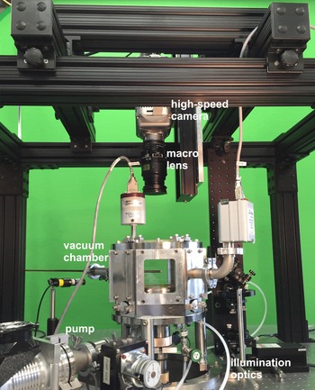
Mounting framework of a high-speed camera above the vacuum chamber. The location of the camera can be adjusted in 3-D, allowing convenient focusing on any location of the dusty plasma suspension.

2.1 Camera and illumination set-up
On the top of the vacuum chamber, we mount two video cameras: a high-speed scientific digital video camera which has a narrow field-of-view (FOV) and serves as the main data-taking device, and wide FOV camera used to survey the entirety of the dust cloud. The latter is generally not used for image analysis, so it can be a less expensive analogue camera. To avoid vibration, these cameras are not suspended in a cantilever configuration, but within a box-like support structure, as shown in figure 1. Preventing vibration is important because camera movement of just a few microns can lead to erroneous measurements of particle velocity. In addition to these top-view cameras, we also use a side-view camera that is positioned at the same height as the dust particles.
A typical scientific camera has a monochrome sensor with of the order of one megapixel resolution. Imaging rates of up to 1000 pictures per second are sometimes needed, although 200 frames
 $\text{s}^{-1}$
, or even less, is more common. A typical example is the Phantom v5.2 shown in figure 1, which has 12 bits of greyscale information in each pixel. Such a camera has an adjustable shutter speed, although with a high frame rate it is common to operate the camera with the longest possible exposure time to achieve a sufficiently bright image. Movies are stored by the camera software as a sequence of bit-map images.
The camera lens is typically a ‘macro’ lens of the kind used for 35 mm film cameras. In our laboratory at Iowa we usually use a 105 mm focal length Nikon lens, as seen in figure 1. The face of the lens is typically positioned approximately 25 cm from the dust cloud; this long working distance is necessary because of the dimensions of the vacuum chamber. A filter is mounted on the entrance of the camera lens; this is typically a 10 nm bandpass filter chosen to admit the wavelength of the laser light used to illuminate the particles, while blocking most of the glow from the plasma.
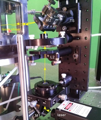
To illuminate the particles, a laser beam is shaped into a fan or sheet of light. In figure 2 a steady-state laser beam, with a power of up to 100 mW, is deflected into a vertical axis where it is focused by a pair of spherical lenses L1 and L2, to achieve a Gaussian focal waist in the centre of the chamber. The beam then passes through a cylindrical lens L3 to disperse the beam into a fan shape. The lens can be rotated, and a subsequent mirror M2 can be tilted and translated to achieve a horizontal orientation for the sheet so that it coincides with the dust particle layer. As an alternative to the cylindrical lens shown in figure 2, it is also possible to raster a laser beam using a high-speed rotating polygonal mirror (Pieper, Goree & Quinn Reference Pieper, Goree and Quinn1996) or a galvanometer mirror that is tilted rapidly back and forth according to a repetitive waveform applied by a function generator (Feng et al. Reference Feng, Goree and Liu2008; Feng, Goree & Liu Reference Feng, Goree and Liu2012a ,Reference Feng, Goree and Liu b ).
Laser illumination optics. A steady-state laser beam is deflected upward by mirror M1 and focused by a telescope consisting of spherical lenses L1 and L2. It is then dispersed into a laser sheet by a cylindrical lens L3 and deflected into a horizontal sheet by mirror M2. This horizontal sheet defines the illuminated volume in the chamber, and it is adjustable using translation stage TS.

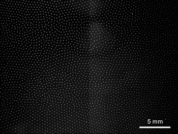
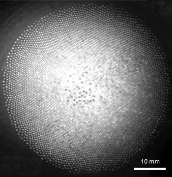
Example top-view images are shown in figures 3 and 4, which are from the narrow FOV and wide FOV cameras, respectively. These images are from the flow experiment of Feng et al. (Reference Feng, Goree and Liu2012a ,Reference Feng, Goree and Liu b ). The narrow FOV camera is pointed near the centre of the particle cloud, where the interparticle distance is fairly uniform; this uniform portion of the dust cloud is ideal to mimic condensed matter with uniform conditions. The wide FOV camera is used to assess the overall cloud shape, and to identify problems such as rapidly moving out-of-plane particles. As seen in figure 4 with the wide FOV camera, the interparticle distance around the edge of the suspension is larger than in the centre; this variation is due to the radial confinement by the naturally present horizontal electric fields in the plasma environment.
Narrow FOV of a 2-D dusty plasma suspension captured from a high-speed camera, Phantom v5.2, on the top the vacuum chamber during the flow experiment of Feng et al. (Reference Feng, Goree and Liu2012a ,Reference Feng, Goree and Liu b ). This image is used for particle identification in our data analysis.

Wide FOV of a 2-D dusty plasma suspension captured from an analogue camera mounted on the top of the vacuum chamber. The corresponding wide FOV movie is used to monitor the whole dusty plasma suspension.

2.2 Camera and illumination adjustment
There are several factors to consider in choosing the intensity of the illuminating laser sheet. It should be bright enough so that all particles can be easily identified. At the same time, the illumination laser should not be too powerful as to push particles noticeably (Liu et al.
Reference Liu, Goree, Nosenko and Boufendi2003)Footnote
1
. After one experimental run, we need to check whether there are any saturated pixels (Feng, Goree & Liu Reference Feng, Goree and Liu2007) in the captured images. It is desirable to avoid large numbers of saturated pixels, because they will spoil the accuracy of the particle position measurement, as described later. In an image with
 ${\sim}10^{3}$
particles each occupying
 ${\sim}20$
pixels, it is acceptable to have a few saturated pixels, but certainly not a few thousand saturated pixels. In the latter case we can correct the problem either by diminishing the illumination power, shortening the exposure time or reducing the aperture of the camera.
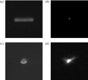
The camera exposure time and frame rate are chosen according to how fast the particles move. In principle, before pixels are saturated, a longer exposure time means accumulating more useful information. However, when particles move quickly, a longer exposure time would result in sausage-shaped images of particles, as in figure 5(a). These sausage-shaped images should be avoided by using a shorter exposure time. Unfortunately, the shorter exposure time can result in an image that is too faint, or it can require using an illuminating laser beam that is too bright so that particles are pushed visibly; this problem arises most often with short exposure times such as
 $10^{-3}$
s. Another approach to avoiding sausage-shaped images is to raster the illuminating laser beam so that it strikes a given dust particle only briefly, instead of illuminating it constantly as when using a cylindrical lens to disperse the light.
Non-ideal particle images: (a) a fast moving particle; (b) low illumination and focused too much; (c) defocused too much exhibiting a ring shape; (d) aperture distortions.

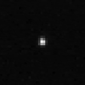
If the particle images are too sharply focused so that they fill only one or two pixels as in figure 5(b), it will be impossible to measure the particle’s position with subpixel accuracy. The camera lens should be adjusted to achieve a sufficiently large spot for each particle. For measuring particle positions, it is best if the image of a particle occupies at least 15–25 pixels to obtain good subpixel accuracy. Diffraction is often sufficient to blur a particle’s image, but if more blurring is needed one can defocus the lens slightly. However, if we defocus the lens too much, as in figure 5(c), the image of one dust particle becomes ring shaped, and this should be avoided. From our experience, the ideal image of one particle should have a circular symmetric shape, occupying 4 to 5 pixels in both
 $x$
and
 $y$
directions, as figure 6 shows. If all the particle images have a similar asymmetric shape, as in figure 5(d), there is a problem in the imaging set-up, for example an irregularly shaped aperture for the camera filter.
An example of the ideal image of one particle. It has a nearly circular symmetric shape, occupying 4 to 5 pixels in both
 $x$
and
 $y$
directions.

3 Analysis techniques
3.1 Dark-field images
The experimenter generally records a dark-field movie along with the main movie, both using the same top-view camera. The main movie shows the particles. The dark-field movie is recorded without particles, but otherwise under exactly the same conditions as the main movie, with both the plasma and illuminating laser turned on. The dark-field images show only camera noise and the background light (for example due to plasma glow and inadvertent laser light reflections in the chamber). By recording of the order of
 $10^{3}$
frames of the dark field, and then averaging them pixel-by-pixel, one generates a dark-field image that is useful for subtraction from each frame of the main movie. This subtraction process can be performed using commonly available software such as ImageJ (Rasband Reference Rasband2016). Using this subtractive process, the images in the main movie are improved to eliminate unwanted background features, so that they are ready for the next step, which is often particle identification.
3.2 Particle identification
Standard image analysis software is used to identify the contiguous pixels that represent an individual particle in the bit-map image of a video frame. Although the particle might be only a few microns in diameter where it is suspended in the plasma, it will appear in the image as a larger spot, due to the effects of diffraction and possibly defocusing of the camera lens, as described above. A particle is identified by the presence of multiple adjacent pixels that are brighter than a specified ‘threshold’ level. One of the advantages of experiments with a monolayer dust cloud is that the images of two particles seldom overlap, so that this particle identification is unambiguous. On the other hand, with 3-D dust clouds, for example in microgravity experiments, sometimes two particles at different distances from the camera can appear to overlap.
Determining the
 $x$
–
 $y$
coordinates of each particle in an image is the central step for particle-level diagnostics of dusty plasmas. There are several methods available to do this, but due to the large number of particles that must be identified (typically
 $10^{3}$
particles in each movie frame and
 $10^{4}$
frames, for a total of the order of
 $10^{7}$
measurements), the measurement must not only be automated, it must also be efficient. The moment method (Feng et al.
Reference Feng, Goree and Liu2007; Ivanov & Melzer Reference Ivanov and Melzer2007) is widely used in dusty plasma experiments to obtain particle positions because it is efficient, and when done properly, it offers great accuracy with errors much smaller than one pixel. In the moment method (Feng et al.
Reference Feng, Goree and Liu2007; Ivanov & Melzer Reference Ivanov and Melzer2007), the particle position is calculated using
 $$\begin{eqnarray}\boldsymbol{X}_{calc}=\frac{\displaystyle \mathop{\sum }_{k}\boldsymbol{X}_{k}w_{k}}{\displaystyle \mathop{\sum }_{k}w_{k}},\end{eqnarray}$$
where
 $\boldsymbol{X}_{k}$
is the coordinate of the pixel
 $k$
belonging to the image of this particle. Our recommended choice for the weighting factor
 $w_{k}$
is the intensity of the pixel minus the threshold level (Feng et al.
Reference Feng, Goree and Liu2007).
There are two sources of errors in calculating particle positions: random and systematic. Random errors can arise from noise in all pixels in experimental images, while systematic errors can arise from the image analysis method, due to the sampling of the imaged light by a rectangular array of pixels. A common systematic error is ‘pixel locking’, which means the computed particle positions tend to have some favourable locations, such as the edge of a pixel or the centre of a pixel. Based on a study that used synthetic images with known true particle positions, Feng et al. (Reference Feng, Goree and Liu2007) developed a recommended practice that minimizes both types of errors simultaneously. Several parts of this recommended practice are mentioned already above: the weighting factor choice for the moment method calculation and the adjustment of the camera lens and laser illumination.
Another part of our recommended practice is the choice of an algorithm for selecting the contiguous pixels that are included in the moment calculation. There is no question that the brightest pixels should be included, but there is considerable freedom in designing an algorithm when selecting which pixels that should be included at the edge of a particle’s image. In Feng et al. (Reference Feng, Goree and Liu2007) several algorithms were tested, and it was found that the one used in ImageJ offered the greatest suppression of pixel-locking errors. This is fortunate, because ImageJ is freely available from the National Institutes of Health (Rasband Reference Rasband2016).
While using the moment method with ImageJ, one key point is making the best choice of the threshold of intensity value to distinguish particles from background noise. The choice of this threshold is tricky (Feng et al. Reference Feng, Goree and Liu2007): it should be low enough to keep enough particle image information, and it should not be too low to wrongly identify noise as particles. In our method, we first subtract the averaged dark-field image from each experimental image pixel-by-pixel as described above and we then use ImageJ to identify particles for the whole movie, requiring as an option in ImageJ that the particle fill multiple pixels. After performing this identification for one value of the threshold, we repeat for various values, and then plot the total number of identified particles versus the corresponding threshold value. In this plot, there is a near-flat portion in the middle range of the threshold value, for example as shown in figure 16 of Feng et al. (Reference Feng, Goree and Liu2007). The desired choice of the threshold should be the lower value of the threshold in this near-flat portion. Further explanation of these steps of selecting the threshold are provided in § VII of Feng et al. (Reference Feng, Goree and Liu2007) with our experimental images.
After identifying particle positions, we test whether pixel locking is a significant problem. This is done using the
 $x$
–
 $y$
coordinates of the particles, in units of pixels. For a measurement of a particle, for example
 $(x,y)=(12.345,67.890)$
, the integer portions of
 $x$
is subtracted, and the same for
 $y$
, yielding the subpixel coordinates, for example
 $(0.345,0.890)$
. Note that in these subpixel coordinates, the possible values of
 $x$
range from 0 to 1, and likewise for
 $y$
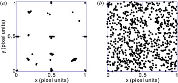
. We repeat for a large number of particle measurements, and then we superimpose the results onto a single graph, which we call a subpixel map. Example subpixel maps from an experiment are shown in figure 7; these examples were prepared from the same data, but with a higher threshold value for figure 7(a) than for figure 7(b). Pixel locking is identified qualitatively by noting whether particles are assigned favoured positions such as the pixel’s middle. We routinely examine subpixel maps like these as one of our considerations when finalizing our choice of the threshold value.
Examples of subpixel maps for calculated particle positions using a higher threshold (a) and a lower threshold (b). In both (a) and (b), approximately 700 particles have been identified within one frame of an experimental image. When the threshold is not suitable as in (a), the subpixel maps reveals pixel locking as a tendency of calculated particle positions to be concentrated at favoured positions such as the centre and edges of pixels. When the threshold is correctly chosen, the subpixel coordinates are much more uniformly distributed within the pixel, as in (b).

3.3 Particle tracking
From identified particle positions, we can track particle motion from one frame to the next, and then compute their velocities. Here we explain the practice that we follow.
To track a particle from one frame to the next, we use simple software, written by ourselves, to search a circular region in the second frame that is centred on the particle’s computed position in the first frame. This search circle has a radius that is a fraction (for example 10 %) of the average interparticle spacing. If exactly one particle is found in the search circle we assume that it is the same one as in the first frame and the tracking is deemed successful, but if there are zero or
 ${>}\!1$
particles in the search circle then the tracking was unsuccessful. The radius of the search circle can be chosen in a compromise to reduce zero-particle outcomes by adjusting the radius upward until there are a few incidents in the movie of
 ${>}\!1$
particles in the search circle.
For many purposes, such as computing particle velocities, it is only necessary to track particles for two consecutive frames. We call this two-frame threading. For other purposes, such as calculating the mean-square displacement of particles over a long time to obtain a diffusion coefficient, it is necessary to track the particles for multiple frames; in this practice of making long threads, a particle will be tracked for only a finite number of frames until it exits from the image or becomes indistinguishable. In experiments with monolayer particle clouds, these problems can be minimized by using a sufficiently high camera frame rate and by analysing only a central region of interest that does not include the edge of the camera image. In experiments with 3-D dust clouds, long threads in 3-D are often impractical due to particles moving in the direction perpendicular to the laser sheet.
The algorithm we use to compute the particle velocity is a simple subtraction of positions in two consecutive frames. This yields a particle velocity
 $$\begin{eqnarray}\boldsymbol{V}_{k+0.5}=(\boldsymbol{X}_{k+1}-\boldsymbol{X}_{k})/t_{frame},\end{eqnarray}$$
where the index
 $k$
represents time and
 $t_{frame}$
is the time interval between the two position measurements. When computing quantities that involve both position and velocity, it is necessary to interpolate the particle positions so that they are recorded simultaneously with the velocity. There are other schemes for determining particle position, but they can all introduce different kinds of errors. We prefer the simple subtractive scheme mentioned above because it is efficient and the errors it generates are understood.
Errors in particle velocities mainly come from two sources (Feng, Goree & Liu Reference Feng, Goree and Liu2011): particle position and particle acceleration. We will discuss these separately. A key experimental parameter, the camera frame rate, actually affects these two kinds of errors in opposite ways, so that minimizing the total error in the particle velocity requires a compromise choice of the frame rate.
Particle position errors, as a source of error in velocity measurement, cause the most severe problems when the particle displacement is small and the frame rate is high, so that the displacement of a particle between two frames is less than the uncertainty of particle positions within a given frame. We can mention two examples of velocity errors due to particle position errors: the low velocity range in a velocity distribution functions can have unphysical oscillations as in figure 4(c) of Nosenko, Goree & Piel (Reference Nosenko, Goree and Piel2006), and calculated velocity autocorrelation function can have a weird shape, as in Feng et al. (Reference Feng, Goree and Liu2011). To minimize this problem, based on our simulation results, we have introduced a method of interlacing pairs of frames to calculate positions and velocities (Feng et al. Reference Feng, Goree and Liu2011): positions are calculated from the average of several consecutive frames, while velocities are calculated from frames with a larger time interval. Superimposing raw data of consecutive frames (Knapek et al. Reference Knapek, Samsonov, Zhdanov, Konopka and Morfill2007) is another method to reduce position and velocity calculation errors. It is interesting to note that a higher frame rate is not always desired for particle tracking in dusty plasma experiments.
Acceleration errors in the velocity determination arise from our definition of velocity in (3.2). This expression assumes that the motion between frames is always a straight line (Feng et al.
Reference Feng, Goree and Liu2011). This assumption works well for a high frame rate since the time scale of dust particle’s motion is much longer than the time interval
 $t_{frame}$
between consecutive frames. However, some information is definitely lost by sampling the particle’s image at fixed time intervals. Causes of particle acceleration in a dusty plasma can include interparticle collisions due to the fluctuating electric fields as individual dust particles approach one another, and cyclotron motion if a strong magnetic field is used. In the latter case, the trajectory of a dust particle is mostly curved, so that our assumption of a straight line between frames may cause substantial systematic errors. In fluid dynamics, spline fit methods (Lüthi, Tsinober & Kinzelbach Reference Lüthi, Tsinober and Kinzelbach2005) have been introduced as an alternative to (3.2) to reduce the systematic error due to this straight line assumption between frames, although a spline fit is much more computationally expensive. Until now, in previous 2-D dusty plasma experiments, we have not noticed substantial systematic errors due to our velocity definition of this straight line assumption between frames.
Note that the time interval when computing velocity in (3.2) need not be the same as the time between frames in the recorded video. We can record data at a higher frame rate, such as 200 to 500 frames
 $\text{s}^{-1}$
, while in later data analysis we can skip frames (Knapek et al.
Reference Knapek, Samsonov, Zhdanov, Konopka and Morfill2007; Feng et al.
Reference Feng, Goree and Liu2011) when using (3.2). Skipping frames in the analysis can be attractive to reduce the velocity error due to errors in particle position measurement, which is likely to be quite significant if the time interval
 $t_{frame}$
is so short that a particle’s displacement is less than 0.3 pixel (Feng et al.
Reference Feng, Goree and Liu2007).
During data analysis, we choose the time interval between frames,
 $t_{frame}$
, according to two schemes that were presented in Feng et al. (Reference Feng, Goree and Liu2011). We summarize one of those schemes here. For velocity measurement, one chooses a value of
 $t_{frame}$
between two limits. The upper limit for
 $t_{frame}$
is significantly smaller than the time scale for the velocity to change significantly in the physical system, for example due to collisions. The lower limit for
 $t_{frame}$
is the accurate pixel resolution size (typically
 ${\sim}0.3$
pixel) divided by the typical speed, such as the thermal speed. In Feng et al. (Reference Feng, Goree and Liu2011), we performed systematic tests of various velocity-related physical quantities to obtain these rules for upper and lower limits.
Finally, we present an example, to illustrate the choice of the time interval for velocity measurement, using the physical quantities in the 2-D strongly coupled dusty plasma experiment of Feng, Goree & Liu (Reference Feng, Goree and Liu2010). In that experiment: the pixel resolution within an image corresponded to
 $30~{\rm\mu}\text{m}$
in the dust cloud, the thermal velocity was about
 $v=1.3~\text{mm}~\text{s}^{-1}$
and a characteristic time scale of a dust particle’s collisional motion was
 ${\it\omega}_{pd}^{-1}=1/30~\text{s}$
. According to the rules above, the time interval between frames for data analysis should have an upper limit of
 $t_{frame}<1/30~\text{s}$
and a lower limit of
 $t_{frame}>(0.3\times 30~{\rm\mu}\text{m})/1.3~\text{mm}~\text{s}^{-1}=0.0069~\text{s}$
. This range of time intervals between frames corresponds to an effective frame rate in the analysis of approximately 30–140 Hz for the experiment of Feng et al. (Reference Feng, Goree and Liu2010). In that experiment we operated the camera at a frame rate of 250 Hz, and in computing the velocity we skipped 1 frame when using (3.2) so that the effective frame rate was
 $1/t_{frame}=125~\text{Hz}$
.
4 Summary
To summarize, we have reviewed imaging diagnostics for measuring particle positions and velocities in dusty plasma experiments. We have summarized our methods to minimize the errors in these measurements. These recommendations are based on our laboratory practice with 2-D dusty plasmas. They can be extended to 3-D dusty plasmas. Based on a recent simulation, Liu, Goree & Suranga Ruhunusiri (Reference Liu, Goree and Suranga Ruhunusiri2015) predicted that our 2-D dusty plasma analysis method introduced here can be used to measure 3-D dusty plasmas with enough accuracy, even when the illumination and imaging uses only a single camera to obtain 2-D cross-sectional images within the 3-D volume.
Acknowledgements
Work in China was supported by the National Natural Science Foundation of China under grant no. 11505124, the 1000 Youth Talents Plan, and the startup funds from Soochow University. Work at the University of Iowa was supported by NSF and the Department of Energy. We thank B. Liu for helpful discussions.