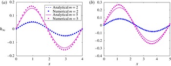
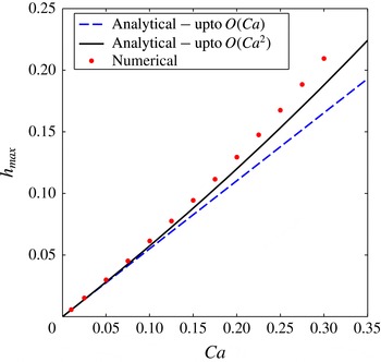
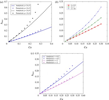
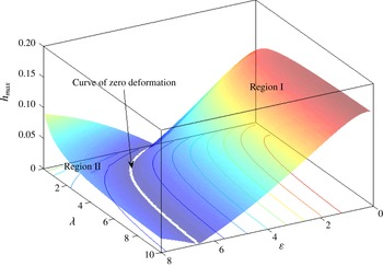
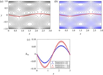
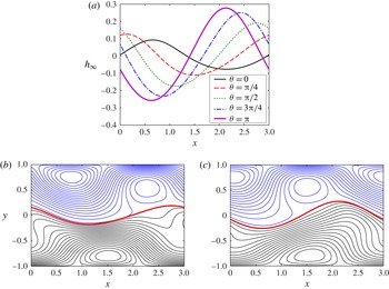
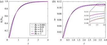
1. Introduction
Electro-osmosis, defined as the motion of fluids in narrow confinements under the action of an axial electric field (Ajdari Reference Ajdari1995, Reference Ajdari1996; Mortensen et al. Reference Mortensen, Olesen, Belmon and Bruus2005; Bahga, Vinogradova & Bazant Reference Bahga, Vinogradova and Bazant2010; Ng & Chu Reference Ng and Chu2011; Ghosh & Chakraborty Reference Ghosh and Chakraborty2012, Reference Ghosh and Chakraborty2013) in the presence of an electric double layer (EDL) near the walls (the walls possess a net charge), has received considerable attention over recent years, due to its wide spectrum of applications, ranging from chip cooling (Stone, Stroock & Ajdari Reference Stone, Stroock and Ajdari2004) to efficient mixing in microchannels (Zhang, He & Liu Reference Zhang, He and Liu2006; Chen & Cho Reference Chen and Cho2007; Chang & Yang Reference Chang and Yang2008; Sugioka Reference Sugioka2010; Ghosh & Chakraborty Reference Ghosh and Chakraborty2012). Recently, researchers have investigated (Mortensen et al. Reference Mortensen, Olesen, Belmon and Bruus2005; Zhang et al. Reference Zhang, He and Liu2006; Chen & Cho Reference Chen and Cho2007; Chang & Yang Reference Chang and Yang2008; Bahga et al. Reference Bahga, Vinogradova and Bazant2010; Sugioka Reference Sugioka2010; Ng & Chu Reference Ng and Chu2011; Ghosh & Chakraborty Reference Ghosh and Chakraborty2012, Reference Ghosh and Chakraborty2013) the effects of non-uniform surface charges (or, equivalently, the surface electrical potential) on the essential features of electro-osmotic flows (EOFs). To this end, one area of particular interest has been the study of EOFs in the presence of patterned periodic surface potentials (Ajdari Reference Ajdari1995, Reference Ajdari2001; Mortensen et al. Reference Mortensen, Olesen, Belmon and Bruus2005; Zhang et al. Reference Zhang, He and Liu2006; Chen & Cho Reference Chen and Cho2007; Chang & Yang Reference Chang and Yang2008; Bahga et al. Reference Bahga, Vinogradova and Bazant2010; Sugioka Reference Sugioka2010; Ng & Chu Reference Ng and Chu2011; Ghosh & Chakraborty Reference Ghosh and Chakraborty2012, Reference Ghosh and Chakraborty2013). A number of previous studies (Ajdari Reference Ajdari1996; Chang & Yang Reference Chang and Yang2008; Ghosh & Chakraborty Reference Ghosh and Chakraborty2012) have demonstrated that interesting flow patterns including large recirculation rolls can be generated with these kinds of modulations, which can be effectively used (Zhang et al. Reference Zhang, He and Liu2006; Chen & Cho Reference Chen and Cho2007; Chang & Yang Reference Chang and Yang2008; Sugioka Reference Sugioka2010; Ghosh & Chakraborty Reference Ghosh and Chakraborty2012) for achieving better mixing in microchannels. It has also been shown that the net throughput in a microchannel can be tuned very finely by superimposing more than one kind of pattern – these include patterned slips (Bahga et al. Reference Bahga, Vinogradova and Bazant2010; Ng & Chu Reference Ng and Chu2011; Ghosh & Chakraborty Reference Ghosh and Chakraborty2012) and topographical patterns (Ajdari Reference Ajdari1996; Chen & Cho Reference Chen and Cho2007), along with the modulations in surface potentials.
However, all of the aforementioned studies mostly concentrate on flows of single-phase fluids through narrow channels. In recent years, electrokinetic flows of multiphase systems, containing liquid–liquid or liquid–air interfaces subjected to uniform and non-uniform electric fields, have gained huge importance (Brask, Kutter & Bruus Reference Brask, Kutter and Bruus2005; Thaokar & Kumaran Reference Thaokar and Kumaran2005; Verma et al. Reference Verma, Sharma, Kargupta and Bhaumik2005; Ozen et al. Reference Ozen, Aubry, Papageorgiou and Petropoulos2006; Tseluiko & Papageorgiou Reference Tseluiko and Papageorgiou2006; Voicu, Harkema & Steiner Reference Voicu, Harkema and Steiner2006; Bandyopadhyay & Sharma Reference Bandyopadhyay and Sharma2007; Tomar et al. Reference Tomar, Shankar, Sharma and Biswas2007; Uguz & Aubry Reference Uguz and Aubry2008; Li, Yin & Yin Reference Li, Yin and Yin2009a ; Gambhire & Thaokar Reference Gambhire and Thaokar2010; Thaokar & Deshmukh Reference Thaokar and Deshmukh2010; Choi et al. Reference Choi, Sharma, Qian, Lim and Joo2011; Esmaeeli & Reddy Reference Esmaeeli and Reddy2011; Zhang, Zahn & Lin Reference Zhang, Zahn and Lin2011; Veremieiev et al. Reference Veremieiev, Thompson, Scholle, Lee and Gaskell2012; Gambhire & Thaokar Reference Gambhire and Thaokar2014) due to their wide range of applications. One of the primary focuses is electro-osmotic pumping of superimposed fluids, first demonstrated experimentally by Brask et al. (Reference Brask, Kutter and Bruus2005). In such systems, a non-conducting fluid with very low electro-osmotic mobility is transported by electro-osmotically actuating a second immiscible conducting fluid with very high electro-osmotic mobility. The non-conducting fluid is transported by the viscous drag at the fluid–fluid interface caused by the motion of the conducting fluid. The pioneering study of Brask et al. (Reference Brask, Kutter and Bruus2005) triggered huge interest in the field of electro-osmotic pumping of non-conducting fluids. As a result, a number of theoretical (Gao et al. Reference Gao, Wong, Yang and Ooi2005; Choi et al. Reference Choi, Sharma, Qian, Lim and Joo2011; Afonso, Alves & Pinho Reference Afonso, Alves and Pinho2013) and experimental studies (Watanabe, Shirai & Hirai Reference Watanabe, Shirai and Hirai2003) have subsequently been executed on this topic. These include analytical investigation for two-fluid electro-osmotic flow at steady state (Choi et al. Reference Choi, Sharma, Qian, Lim and Joo2011; Mayur et al. Reference Mayur, Amiroudine, Lasseux and Chakraborty2013) and transience (Gao et al. Reference Gao, Wong, Yang and Ooi2005; Haiwang, Wong & Nguyen Reference Haiwang, Wong and Nguyen2010), and analytical solutions for electro-osmotic flow of superimposed viscoelastic fluids (Afonso et al. Reference Afonso, Alves and Pinho2013), to name a few. In recent years, researchers have further looked into the effects of interfacial electrostatics on the electro-osmosis of two-fluid systems. Choi et al. (Reference Choi, Sharma, Qian, Lim and Joo2011) investigated the effects of potential jump across the interface in a two-fluid system, while also taking into account the effects of charge accumulation at the interface. Mayur et al. (Reference Mayur, Amiroudine, Lasseux and Chakraborty2013) studied the effects of Maxwell stresses acting at a liquid–gas interface on electro-osmotic flow of the liquid. Experimental investigations have also been performed (Watanabe et al. Reference Watanabe, Shirai and Hirai2003) on the effects of fluid properties, interfacial potential and salt concentrations on the characteristics of two-fluid electro-osmotic pumps. In addition to pumps for non-conducting liquids, electro-osmotic flow of multiple immiscible fluid layers also has major applications in the fields of valveless flow switching (Li, Wong & Nguyen Reference Li, Wong and Nguyen2010b ) in microfluidic channels, development of finely tunable micro-optofluidic lenses (Li, Wong & Nguyen Reference Li, Wong and Nguyen2010a ), hydrodynamic flow focusing and controlling stream width (Li, Wong & Nguyen Reference Li, Wong and Nguyen2009b ), manoeuvring of interface location and residence time, to name a few. Previous experimental studies (Wang et al. Reference Wang, Gao, Nguyen, Wong, Yang and Ooi2005; Gao et al. Reference Gao, Wang, Wong, Yang, Nguyen and Ooi2007; Li et al. Reference Li, Wong and Nguyen2009b ) have demonstrated that the location of the interface and the stream width can be finely tuned by adjusting the externally applied electric field in a combined pressure-driven and electro-osmotic flow of a triple-fluid-layer system. Li et al. (Reference Li, Wong and Nguyen2010a ,Reference Li, Wong and Nguyen b ) have shown that the optical properties of a microfluidic lens are strongly dependent on the shape of the interface, which in turn can be controlled by adjusting the applied external electric field. Their experimental results show that, depending on the field strength, various interfacial shapes, like planoconvex, biconvex, etc. can be created. Most of these experimental studies employ three immiscible layers of fluids, where a non-conducting fluid layer is sandwiched between two conducting liquids. Additionally, almost all of the aforementioned studies consider uniform surface potentials for theoretical estimations, and therefore a flat liquid–liquid interface is automatically assumed.
Focusing particularly on the electrohydrodynamics of superimposed fluids in the presence of a modulated surface potential, such systems have been shown (Schäffer et al. Reference Schäffer, Thurn-Albrecht, Russell and Steiner2000, Reference Schäffer, Thurn-Albrecht, Russell and Steiner2001; Verma et al. Reference Verma, Sharma, Kargupta and Bhaumik2005; Yeoh, Xu & Basaran Reference Yeoh, Xu and Basaran2007; Esmaeeli & Reddy Reference Esmaeeli and Reddy2011) to cause interesting pattern formation. The pioneering work of Schäffer et al. (Reference Schäffer, Thurn-Albrecht, Russell and Steiner2000) demonstrated that application of a non-uniform electric field can lead to the formation of pillar-like patterns replicating the shapes of the electrodes in thin polymeric films. Later, Yeoh et al. (Reference Yeoh, Xu and Basaran2007) theoretically predicted that the liquid interface always gets deformed when subjected to a non-uniform potential. Theoretical estimations of flows caused by imbalances in Maxwell stresses and the resulting deformation, in the presence of a patterned surface potential (Esmaeeli & Reddy Reference Esmaeeli and Reddy2011) and topography (Tseluiko et al. Reference Tseluiko, Blyth, Papageorgiou and Vanden-Broeck2008a ,Reference Tseluiko, Blyth, Papageorgiou and Vanden-Broeck b ), have been reported in the literature. It has been shown that a high magnitude of non-uniform electric field can lead to significant alteration in the film shape (Schäffer et al. Reference Schäffer, Thurn-Albrecht, Russell and Steiner2000; Wu & Russel Reference Wu and Russel2005) and can potentially lead to instabilities (Schäffer et al. Reference Schäffer, Thurn-Albrecht, Russell and Steiner2001; Thaokar & Kumaran Reference Thaokar and Kumaran2005; Verma et al. Reference Verma, Sharma, Kargupta and Bhaumik2005; Gambhire & Thaokar Reference Gambhire and Thaokar2014). Such instabilities are termed electrohydrodynamic instabilities, or, EHDIs. Several thin-film patterns have been successfully generated experimentally (Schäffer et al. Reference Schäffer, Thurn-Albrecht, Russell and Steiner2000, Reference Schäffer, Thurn-Albrecht, Russell and Steiner2001; Voicu et al. Reference Voicu, Harkema and Steiner2006) using these instabilities. Schäffer et al. (Reference Schäffer, Thurn-Albrecht, Russell and Steiner2001) have demonstrated that various stages of instabilities in thin polymer films can be obtained by controlling the magnitude of the applied electric field. An excellent review of micro- and nano-pattern formation in thin films by employing EHDIs can be found in the work of Wu & Russel (Reference Wu and Russel2009). A number of previous numerical studies (Verma et al., Reference Verma, Sharma, Kargupta and Bhaumik2005 and references therein) have also demonstrated that various shapes and patterns in thin films can be created using the EHDIs, by simply varying the magnitude of the applied electric field.
However, most of the theoretical studies on the electrohydrodynamics of superimposed fluids, in the presence of a patterned potential, either consider the leaky dielectric model (proposed by Melcher & Taylor Reference Melcher and Taylor1969), without any imposed flow, or only study the equilibrium profile of the interface (Yeoh et al. Reference Yeoh, Xu and Basaran2007). The aforementioned studies did not consider any axially applied electric field and hence no imposed electro-osmotic flow was present in these cases. All the flow structures thus reported were outcomes of the interfacial deformation itself. In addition to this, the leaky dielectric model, used in these studies, is limited to fluids with very small conductivities (e.g. silicone oil, castor oil). Thus, a more general model would be to consider fluids and/or electrolyte solutions with high conductivity which can contain net charges. These fluids can be subjected to electro-osmotic flows by applying a net electric field in the axial direction. However, previous studies on electro-osmotic flows of superimposed fluids have only considered uniform surface potential, which implies a flat interface shape. Extrapolating the already reported work on electro-osmotic flows in the presence of a patterned surface potential, it can be very easily inferred that, for superimposed two-fluid systems, such flows can offer a wealth of interesting features, many of which are yet to be addressed properly. Keeping this in mind, in the present analysis we focus on the deformation caused by an imposed electro-osmotic flow generated by an axially applied electric field in the presence of a modulated surface potential on the channel walls, under a thin-EDL approximation. In an effort to mimic physically realistic systems, we consider the two fluids to have different properties, such as viscosities and permittivities. We analyse the combined effect of hydrodynamic and Maxwell stresses on the flow dynamics and interface shape, in the presence of a patterned surface potential. In an effort to keep the analysis focused, we assume that no charge accumulation occurs at the interface. The present analysis can be largely divided into two parts: in the first part we attempt to find approximate analytical solutions to the aforementioned problem, whereas in the following part a numerical technique is applied to solve the full system of relevant equations to obtain solutions with a larger range of parameters. The analytical solutions are derived assuming the effects of inertia on the flow dynamics to be negligible. Thus, the analytical solutions only focus on the transient deformation process, while the fluid flow is assumed to be quasisteady at all times. The numerical simulations are performed using the widely used phase field formalism (Anderson, McFadden & Wheeler Reference Anderson, McFadden and Wheeler1998; Jacqmin Reference Jacqmin1999; Badalassi, Ceniceros & Banerjee Reference Badalassi, Ceniceros and Banerjee2003; Chaudhury, Ghosh & Chakraborty Reference Chaudhury, Ghosh and Chakraborty2013; Mondal et al. Reference Mondal, Ghosh, Bandopadhyay, DasGupta and Chakraborty2013; Sibley, Nold & Kalliadasis Reference Sibley, Nold and Kalliadasis2013; Mondal, DasGupta & Chakraborty Reference Mondal, DasGupta and Chakraborty2014a ; Mondal et al. Reference Mondal, Ghosh, Bandopadhyay, DasGupta and Chakraborty2014b ), where the effects of inertia on the flow dynamics are included. Our analysis reveals that the deformation shows a simple sinusoidal variation for low capillary numbers (Ca) (for the potential pattern considered in the present study), although for higher Ca, more complex variations are witnessed. We also show that the deformation of the interface can be augmented as well as suppressed by adjusting geometric as well as physical properties of the fluid, such as viscosity, permittivity, etc. We further highlight that a reasonably good agreement is observed between the numerical and analytical solutions in the present study.
2. Problem formulation
2.1. System description
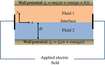
Our system consists of two superimposed immiscible fluids, confined between two parallel plates, located at
 $y=-H$
and
 $y=H$
, as depicted schematically in figure 1. The
 $x$
axis runs along the channel. We denote the fluid on top as fluid 1 and that at the bottom as fluid 2. The viscosity, density and permittivity of the fluids are given by
 ${\it\eta}_{i}$
,
 ${\it\rho}_{i}$
and
 ${\it\varepsilon}_{i}$
respectively, where
 $i=1$
denotes fluid 1 and
 $i=2$
denotes fluid 2. We define the following parameters for the fluid property ratios: viscosity ratio
 ${\it\lambda}={\it\eta}_{1}/{\it\eta}_{2}$
, permittivity ratio
 ${\it\varepsilon}={\it\varepsilon}_{1}/{\it\varepsilon}_{2}$
and density ratio
 $\bar{{\it\rho}}={\it\rho}_{1}/{\it\rho}_{2}$
. We assume both the fluids to be perfect dielectrics. Initially, we consider the interface between the fluids to be flat and located along
 $y=0$
. The surface tension at the interface is assumed to be
 ${\it\sigma}$
.
Schematic of the system under consideration: two fluids sandwiched between two parallel plates. An electric field is applied in the axial direction, which actuates the flow. The interface originally lies flat at
 $y=0$
. The potentials on the walls are modulated. The potentials on the two walls are, in general, not equal, unless
 $m=1$
, which creates an asymmetry in the domain.

Both the walls bear a potential, which is given for the bottom wall as
 ${\it\zeta}_{b}(x)={\it\zeta}_{0}(n+\cos (qx))$
and for the top wall as
 ${\it\zeta}_{t}(x)=m{\it\zeta}_{0}(n+\cos (qx+{\it\theta}))$
, where
 ${\it\theta}$
is the phase shift angle between the potentials at the two walls. We assume both
 $n$
and
 $m$
to be
 $O(1)$
constants. In the present work we consider the existence of EDLs near both the walls, which can be generated by mixing electrolytes with the liquids. We assume the channel height to be large enough so that the thin-EDL approximation remains valid. An axial electric field, with potential drop
 $V$
per modulation wavelength (
 $d=2{\rm\pi}/q$
), is applied along the channel, to actuate electro-osmotic flow. In general, the flow thus created will tend to deform the interface due to the presence of axially periodic components in the potential, which, in turn, will influence the flow. In the present study, we intend to find the deformed shape of the interface as well as the resulting flow patterns for the aforementioned system configurations. Since we are going to consider slow motion of liquids through narrow confinements, the deformation in the present case will be a strong function of the capillary number, defined as
 $\mathit{Ca}={\it\eta}_{2}u_{c}/{\it\sigma}$
, where
 $u_{c}$
is the characteristic velocity and
 ${\it\sigma}$
is the coefficient of surface tension.
Before we move on to the detailed formulation, it is important to mention the associated assumptions made to execute the analysis. First, we assume the thin-EDL limit to be valid (as mentioned in the previous paragraph), so that the Smoluchowski slip velocity conditions can be applied at the walls. In order for the slip velocity condition to be valid, we must meet several criteria, which include low to moderate value of the ionic Péclet number, low surface potential and low surface conductance (Squires & Bazant Reference Squires and Bazant2004), and we assume that all these conditions are satisfied for the present analysis. Second, we assume the Reynolds number (Re) to be small enough that the inertial terms in the Navier–Stokes equations can be safely neglected for the analytical solution. Third, we assume that the time scale of deformation for the interface is much larger than the time scale for the flow to reach steady state. As we show subsequently, the ratio of these two scales is given by the Ohnesorge number (Mandal, Chaudhury & Chakraborty Reference Mandal, Chaudhury and Chakraborty2014) (defined as
 $\mathit{Oh}={\it\eta}_{2}/\sqrt{{\it\rho}_{2}{\it\sigma}H}$
). Therefore, in the present study we assume
 $\mathit{Oh}^{2}\gg 1$
. This assumption enables us to resolve the evolution of the interface in time, although the transience in the flow cannot be captured under these conditions, which, in other words, primarily indicates that the fluid instantaneously adjusts to any changes in the interface shape with time. Finally, we will assume that the gravitational effects are small enough to be neglected from the analysis.
We first present the general governing equations and boundary conditions for the system as described above. We then obtain approximate analytical solutions from these equations for the deformation and the flow structure using asymptotic methods (domain perturbation) in the limit of small deformation
 $(\mathit{Ca}\ll 1)$
. We further assume
 ${\it\theta}=0$
for the analytical solutions. In the next section we attempt to solve for the flow structure and the interface shape numerically over a wide range of governing parameters (
 $\mathit{Ca},{\it\lambda},{\it\varepsilon}$
and
 $q$
), albeit within the framework of low Re and the thin-EDL limit. Towards this end, we employ a diffuse interface model (Badalassi et al.
Reference Badalassi, Ceniceros and Banerjee2003) (phase field model), where an order parameter is defined to denote the two fluids. We then solve the coupled Cahn–Hilliard–Navier–Stokes equations (Badalassi et al.
Reference Badalassi, Ceniceros and Banerjee2003) to obtain the distribution of the order parameter and flow profile, which subsequently gives us the interface shape. In § 5, we compare our approximate analytic solutions with the numerical solutions for small values of the capillary number and execute a parametric study of the parameters responsible for changes in the flow dynamics. Finally, we conclude this work in § 6 and discuss possible future extensions.
2.2. Governing equations
The equations of motion for the two fluids in the limit of thin EDL are given by the Navier–Stokes equation in the following form:
 $$\begin{eqnarray}{\it\rho}_{i}\frac{\text{D}\boldsymbol{v}_{\boldsymbol{i}}}{\text{D}t}=-\boldsymbol{{\rm\nabla}}p_{i}+{\it\eta}_{i}{\rm\nabla}^{2}\boldsymbol{v}_{i},\quad i=1,2,\end{eqnarray}$$
where
 $\boldsymbol{v}_{\boldsymbol{i}}=(u_{i},v_{i})$
represents the velocity field. The subscript ‘
 $i$
’ denotes the
 $i$
th fluid. The fluid velocities also have to satisfy the continuity equation in the following form:
 $$\begin{eqnarray}\boldsymbol{{\rm\nabla}}\boldsymbol{\cdot }\boldsymbol{v}_{i}=0.\end{eqnarray}$$
The potential for the axially applied electric field satisfies the following equation (Ajdari Reference Ajdari1995):
 $$\begin{eqnarray}{\it\varepsilon}_{1}{\rm\nabla}^{2}{\it\varphi}_{1}={\it\varepsilon}_{2}{\rm\nabla}^{2}{\it\varphi}_{2}=0.\end{eqnarray}$$
In (2.3),
 ${\it\varphi}_{i}$
denotes the potential in the
 $i$
th fluid. The axial electric field is thus given by
 $$\begin{eqnarray}\boldsymbol{E}_{i}=-\boldsymbol{{\rm\nabla}}{\it\varphi}_{i}.\end{eqnarray}$$
The fluid velocities and the potential are subject to the following boundary conditions. At the walls the applied potential will satisfy (Ajdari Reference Ajdari1995)
 $$\begin{eqnarray}\frac{\partial {\it\varphi}_{1}}{\partial y}=0\quad \text{at}~y=H\quad \text{and}\quad \frac{\partial {\it\varphi}_{2}}{\partial y}=0\quad \text{at}~y=-H.\end{eqnarray}$$
At the walls the
 $x$
velocities satisfy the Smoluchowski slip velocity condition (Ajdari Reference Ajdari1996), as attributable to the thin-EDL regime we consider here. Therefore,
 $$\begin{eqnarray}\displaystyle & \displaystyle u_{1}=\frac{{\it\varepsilon}_{1}{\it\zeta}_{t}(x)}{{\it\eta}_{1}}\frac{\partial {\it\varphi}_{1}}{\partial x}\quad \text{and}\quad v_{1}=0\quad \text{at}~y=H, & \displaystyle\end{eqnarray}$$
 $$\begin{eqnarray}\displaystyle & \displaystyle u_{2}=\frac{{\it\varepsilon}_{2}{\it\zeta}_{b}(x)}{{\it\eta}_{2}}\frac{\partial {\it\varphi}_{2}}{\partial x}\quad \text{and}\quad v_{2}=0\quad \text{at}~y=-H. & \displaystyle\end{eqnarray}$$
At the interface, the tangential components of the axial electric field and the normal component of the displacement field will be continuous, since we assume the fluids to be perfect dielectrics. On the other hand, the velocities have to satisfy the no-slip and kinematic conditions, as well as the tangential and normal stress balance criterion (Leal Reference Leal2007). Since the interface shape is a priori unknown and it will be deformed in general due to the imbalance of normal stresses, we assume that the interface shape is given by the following equation:
 $$\begin{eqnarray}F\equiv y-h(x,t)=0.\end{eqnarray}$$
Since we consider the transient interface deformation, the interface height is taken as a function of both the
 $x$
coordinate and time. In the present case, the aforementioned boundary conditions take the following form at the interface.
Continuity of tangential electric field:
 $$\begin{eqnarray}\displaystyle {\it\varphi}_{1}={\it\varphi}_{2}\quad \text{at}~y=h(x,t). & & \displaystyle\end{eqnarray}$$
Continuity of normal displacement field:
 $$\begin{eqnarray}\displaystyle {\it\varepsilon}_{1}\boldsymbol{n}\boldsymbol{\cdot }\boldsymbol{{\rm\nabla}}{\it\varphi}_{1}={\it\varepsilon}_{2}\boldsymbol{n}\boldsymbol{\cdot }\boldsymbol{{\rm\nabla}}{\it\varphi}_{2}\quad \text{at}~y=h(x,t). & & \displaystyle\end{eqnarray}$$
No-slip condition:
 $$\begin{eqnarray}\displaystyle \boldsymbol{v}_{1}\boldsymbol{\cdot }\hat{\boldsymbol{t}}=\boldsymbol{v}_{2}\boldsymbol{\cdot }\hat{\boldsymbol{t}}\quad \text{at}~y=h(x,t). & & \displaystyle\end{eqnarray}$$
Kinematic condition:
 $$\begin{eqnarray}\displaystyle \frac{1}{\left|\boldsymbol{{\rm\nabla}}F\right|}\frac{\partial F}{\partial t}+\boldsymbol{v}_{\boldsymbol{i}}\boldsymbol{\cdot }\hat{\boldsymbol{n}}=0,\quad i=1,2,~\text{at}~y=h(x,t). & & \displaystyle\end{eqnarray}$$
Shear stress balance:
 $$\begin{eqnarray}\displaystyle ({\bf\tau}_{1}\boldsymbol{\cdot }\hat{\boldsymbol{n}})\boldsymbol{\cdot }\hat{\boldsymbol{t}}=({\bf\tau}_{2}\boldsymbol{\cdot }\hat{\boldsymbol{n}})\boldsymbol{\cdot }\hat{\boldsymbol{t}}\quad \text{at}~y=h(x,t). & & \displaystyle\end{eqnarray}$$
Normal stress balance:
 $$\begin{eqnarray}\displaystyle p_{1}-p_{2}+\left[\left({\bf\tau}_{2}-{\bf\tau}_{1}\right)\boldsymbol{\cdot }\hat{\boldsymbol{n}}\right]\boldsymbol{\cdot }\hat{\boldsymbol{n}}=-{\it\sigma}\boldsymbol{{\rm\nabla}}_{\boldsymbol{s}}\boldsymbol{\cdot }\hat{\boldsymbol{n}}\quad \text{at}~y=h(x,t). & & \displaystyle\end{eqnarray}$$
Along the axial direction, the applied potential
 ${\it\varphi}_{i}$
will satisfy the following conditions:
 $$\begin{eqnarray}\text{at}~x=0,\quad {\it\varphi}_{i}=0\quad \text{and}\quad \text{at}~x=d,\quad {\it\varphi}_{i}=-V,~i=1,2.\end{eqnarray}$$
In (2.4k
)
 $d$
is the modulation wavelength, given by
 $d=2{\rm\pi}/q$
. This condition basically indicates the potential drop along a single modulation. In conditions (2.4e
)–(2.4j
),
 $\hat{\boldsymbol{n}}$
(directed from fluid 2 to fluid 1) and
 $\hat{\boldsymbol{t}}$
denote normal and tangent unit vectors to the interface respectively. Additionally,
 ${\bf\tau}_{i}$
denotes the stress tensor in the
 $i$
th fluid,
 ${\it\sigma}$
is the surface tension and
 $\boldsymbol{{\rm\nabla}}_{\boldsymbol{s}}$
denotes the surface gradient operator, which has the following expression:
 $\boldsymbol{{\rm\nabla}}_{\boldsymbol{s}}=\boldsymbol{{\rm\nabla}}-\hat{\boldsymbol{n}}(\hat{\boldsymbol{n}}\boldsymbol{\cdot }\boldsymbol{{\rm\nabla}})$
. The rest of the symbols bear their usual meanings. It should be noted that the stress tensors include contributions from Maxwell as well as viscous stresses, expressed as
 $$\begin{eqnarray}{\bf\tau}={\it\eta}\left[\boldsymbol{{\rm\nabla}}\boldsymbol{v}+(\boldsymbol{{\rm\nabla}}\boldsymbol{v})^{\text{T}}\right]+{\it\varepsilon}(\boldsymbol{E}\boldsymbol{E}-{\textstyle \frac{1}{2}}(\boldsymbol{E}\boldsymbol{\cdot }\boldsymbol{E})\boldsymbol{I}).\end{eqnarray}$$
In (2.5),
 $\boldsymbol{E}$
is the applied electric field given by (2.3b
). We shall denote the hydrodynamic part of the stress by
 ${\bf\tau}^{(\boldsymbol{h})}$
and the Maxwell stress by
 ${\bf\tau}^{(\boldsymbol{e})}$
. In view of the boundary conditions at the walls and taking into account the fact that the surface potentials are periodic in nature along the axial directions, we consider all the quantities to be periodic along the
 $x$
axis, which remains a standard assumption in EOF in the presence of charge-modulated surface conditions (Ajdari Reference Ajdari1996; Ghosh & Chakraborty Reference Ghosh and Chakraborty2012).
We now non-dimensionalize the governing equations, where the characteristic scale for each variable is used as the reference value so as to make the non-dimensional variables
 $O(1)$
. Towards this end, we define, for any variable
 ${\it\chi}$
,
 $\bar{{\it\chi}}={\it\chi}/{\it\chi}_{c}$
, where
 ${\it\chi}_{c}$
is the characteristic value. As characteristic values, we chose the characteristic electric field magnitude as
 $E_{0}=V/d$
, the characteristic velocity as
 $u_{c}={\it\varepsilon}_{2}E_{0}{\it\zeta}_{0}/{\it\eta}_{2}$
, the characteristic lengths as
 $x_{c}=y_{c}=H$
and the characteristic potential as
 ${\it\varphi}_{c}=V$
. The characteristic hydrodynamic stress is chosen as
 ${\it\tau}_{c}^{(h)}={\it\eta}_{2}u_{c}/H$
and
 $p_{c}={\it\tau}_{c}^{(h)}$
, while the characteristic Maxwell stress is chosen as
 ${\it\tau}_{c}^{(e)}={\it\varepsilon}_{2}E_{0}^{2}$
. The ratio of the two stresses is taken as
 ${\it\tau}_{c}^{(e)}/{\it\tau}_{c}^{(e)}=(E_{0}H)/{\it\zeta}_{0}={\it\beta}$
. With the above choices of characteristic variables, the non-dimensional electric field is defined as
 $$\begin{eqnarray}\bar{\boldsymbol{E}}_{i}=-\bar{d}\boldsymbol{{\rm\nabla}}\bar{{\it\varphi}}_{i}.\end{eqnarray}$$
Previous studies (see Mandal et al.
Reference Mandal, Chaudhury and Chakraborty2014 and the references therein) have demonstrated that the time scale for deformation of the interface is of the order of
 $t_{c}\sim \mathit{Ca}(H/u_{c})$
(
 $\mathit{Ca}$
is the capillary number, as defined earlier). Therefore, we chose this scale as the characteristic value of the time. It can be easily understood that for
 $\mathit{Ca}\ll 1$
, this scale is much smaller than the advective time scale for fluid flows. We also note that we have chosen the length scales in both directions to be the same, which indicates that the modulation wavelength (
 $d=2{\rm\pi}/q$
) must be of the same order as the channel height (or half-height). Enforcing the aforementioned non-dimensionalization scheme, we obtain the following non-dimensional equations:
 $$\begin{eqnarray}\displaystyle & \displaystyle \bar{{\it\rho}}\left\{\frac{1}{\mathit{Oh}^{2}}\frac{\partial \boldsymbol{v}_{1}}{\partial t}+\mathit{Re}(\boldsymbol{v}_{1}\boldsymbol{\cdot }\boldsymbol{{\rm\nabla}}\boldsymbol{v}_{1})\right\}=-\boldsymbol{{\rm\nabla}}p_{1}+{\it\lambda}{\rm\nabla}^{2}\boldsymbol{v}_{1}, & \displaystyle\end{eqnarray}$$
 $$\begin{eqnarray}\displaystyle & \displaystyle \frac{1}{\mathit{Oh}^{2}}\frac{\partial \boldsymbol{v}_{2}}{\partial t}+\mathit{Re}(\boldsymbol{v}_{2}\boldsymbol{\cdot }\boldsymbol{{\rm\nabla}}\boldsymbol{v}_{2})=-\boldsymbol{{\rm\nabla}}p_{2}+{\rm\nabla}^{2}\boldsymbol{v}_{2}, & \displaystyle\end{eqnarray}$$
along with the continuity equation in the form
 $$\begin{eqnarray}\displaystyle \boldsymbol{{\rm\nabla}}\boldsymbol{\cdot }\boldsymbol{v}_{\boldsymbol{i}}=0. & & \displaystyle\end{eqnarray}$$
The potentials satisfy
 $$\begin{eqnarray}\displaystyle {\rm\nabla}^{2}{\it\varphi}_{2}={\it\varepsilon}{\rm\nabla}^{2}{\it\varphi}_{1}=0,\quad i=1,2. & & \displaystyle\end{eqnarray}$$
It should be noted that we have used the same symbols for the non-dimensional variables as the dimensional ones, since (unless otherwise mentioned) we will be using the non-dimensional variables throughout the present study. The boundary conditions take the following forms:
 $$\begin{eqnarray}\displaystyle & {\it\varphi}_{1}={\it\varphi}_{2}\quad \text{at}~y=h(x,t), & \displaystyle\end{eqnarray}$$
 $$\begin{eqnarray}\displaystyle & {\it\varepsilon}\hat{\boldsymbol{n}}\boldsymbol{\cdot }\boldsymbol{{\rm\nabla}}{\it\varphi}_{1}=\hat{\boldsymbol{n}}\boldsymbol{\cdot }\boldsymbol{{\rm\nabla}}{\it\varphi}_{2}\quad \text{at}~y=h(x,t), & \displaystyle\end{eqnarray}$$
 $$\begin{eqnarray}\displaystyle & \boldsymbol{v}_{1}\boldsymbol{\cdot }\hat{\boldsymbol{t}}=\boldsymbol{v}_{2}\boldsymbol{\cdot }\hat{\boldsymbol{t}}\quad \text{at}~y=h(x,t), & \displaystyle\end{eqnarray}$$
 $$\begin{eqnarray}\displaystyle & \displaystyle \frac{1}{\mathit{Ca}\left|\boldsymbol{{\rm\nabla}}F\right|}\frac{\partial F}{\partial t}+\boldsymbol{v}_{\boldsymbol{i}}\boldsymbol{\cdot }\hat{\boldsymbol{n}}=0,\quad i=1,2,~\text{at}~y=h(x,t), & \displaystyle\end{eqnarray}$$
 $$\begin{eqnarray}\displaystyle & \left({\bf\tau}_{1}\boldsymbol{\cdot }\hat{\boldsymbol{n}}\right)\boldsymbol{\cdot }\hat{\boldsymbol{t}}=({\bf\tau}_{2}\boldsymbol{\cdot }\hat{\boldsymbol{n}})\boldsymbol{\cdot }\hat{\boldsymbol{t}}\quad \text{at}~y=h(x,t), & \displaystyle\end{eqnarray}$$
 $$\begin{eqnarray}\displaystyle & \displaystyle p_{1}-p_{2}+\left[({\bf\tau}_{2}-{\bf\tau}_{1})\boldsymbol{\cdot }\hat{\boldsymbol{n}}\right]\boldsymbol{\cdot }\hat{\boldsymbol{n}}=-\frac{1}{\mathit{Ca}}\boldsymbol{{\rm\nabla}}_{\boldsymbol{s}}\boldsymbol{\cdot }\hat{\boldsymbol{n}}\quad \text{at}~y=h(x,t). & \displaystyle\end{eqnarray}$$
 ${\bf\tau}_{i}={\bf\tau}_{i}^{(\boldsymbol{h})}+{\it\beta}{\bf\tau}_{\boldsymbol{i}}^{(\boldsymbol{e})}$
, for
 $i=1,2$
. As mentioned earlier, in the present study we consider the cases where
 $\mathit{Oh}\gg 1$
and
 $\mathit{Re}\ll 1$
. Enforcing these approximations, (2.7a
) and (2.7b
) become
 $$\begin{eqnarray}\displaystyle & 0=-\boldsymbol{{\rm\nabla}}p_{1}+{\it\lambda}{\rm\nabla}^{2}\boldsymbol{v}_{1}, & \displaystyle\end{eqnarray}$$
 $$\begin{eqnarray}\displaystyle & 0=-\boldsymbol{{\rm\nabla}}p_{2}+{\rm\nabla}^{2}\boldsymbol{v}_{2}. & \displaystyle\end{eqnarray}$$
 $h(x,t)$
is not known a priori and has to be determined as part of the solution.
3. Approximate analytical solutions
Although (2.9a
)–(2.9b
) and (2.7c
)–(2.7d
) and conditions (2.8a
)–(2.8f
) are significantly simpler than the full-scale problem, they are still not analytically tractable for arbitrary Ca. However, for small values of Ca, one can assume the deformation to be small and perform an asymptotic analysis to find approximate solutions for the velocity profile and the deformation. Towards this end we expand all the dependent variables in a power series of Ca and apply domain perturbation at the interface to determine the solutions at successive orders. For any variable
 ${\it\chi}$
we write
 $$\begin{eqnarray}{\it\chi}={\it\chi}^{(0)}+\mathit{Ca}{\it\chi}^{(1)}+\mathit{Ca}^{2}{\it\chi}^{(2)}+\cdots \,.\end{eqnarray}$$
Here,
 ${\it\chi}$
represents variables like
 $u_{1}$
,
 $v_{1}$
,
 $u_{2}$
,
 $v_{2}$
,
 $h(x,t)$
, etc. Since in the leading order the interface remains flat, the expansion for the deformation becomes
 $$\begin{eqnarray}h(x,t)=\mathit{Ca}h_{1}(x,t)+\mathit{Ca}^{2}h_{2}(x,t)+\cdots \,.\end{eqnarray}$$
A review of the relevant literature on deformation of fluid–fluid interfaces for low capillary numbers (Leal Reference Leal2007; Ramachandran & Leal Reference Ramachandran and Leal2012) suggests that the boundary conditions (2.8a
)–(2.8f
) are sufficient to completely specify the velocity field in terms of the deformation height (for unsteady flows), while the remaining condition ((2.8f
), normal stress balance) gives us the closed-form expression for the deformation. The nature of condition (2.8f
) therefore suggests that in order to obtain the
 $O(\mathit{Ca})$
deformation one only needs to solve the leading-order velocity, and so on for the higher orders in Ca. A number of previous studies (Chan & Leal Reference Chan and Leal2006; Leal Reference Leal2007; Ramachandran & Leal Reference Ramachandran and Leal2012) on interface deformation in two-fluid systems have reported good agreement between the experimental results and numerical simulations, with the analytic solutions using the method outlined above.
We note that in the present analysis the capillary number plays a very important role, since it is one of the main factors controlling the deformation. Thus, we discuss the possible range of values that this number can assume for the present analysis. With the choice of reference velocity as mentioned in § 2, the expression for Ca finally becomes
 $\mathit{Ca}=({\it\varepsilon}_{2}E_{0}{\it\zeta}_{0})/{\it\sigma}$
. Therefore, depending on the values of the fluid properties, applied field and surface potential, the capillary number may have a wide range of values. More quantitatively, assuming the bottom fluid to be an aqueous solution, we take
 ${\it\varepsilon}_{2}\sim 7\times 10^{-10}~\text{F}~\text{m}^{-1}$
. Therefore, for typical zeta potentials in the range
 ${\it\zeta}_{0}\sim 10$
to 100 mV, one can write
 $\mathit{Ca}\sim 7\times 10^{-12}\times (E_{0}/{\it\sigma})$
to
 $7\times 10^{-11}\times (E_{0}/{\it\sigma})$
. For relatively high values of the applied axial electric field,
 $E_{0}\sim 5000~\text{kV}~\text{m}^{-1}$
(note that in previous literature even higher values of the applied electric fields have been considered (Schäffer et al.
Reference Schäffer, Thurn-Albrecht, Russell and Steiner2001; Das et al.
Reference Das, Dubsky, van den Berg and Eijkel2012)), and low surface tension,
 ${\it\sigma}\sim 10^{-3}~\text{N}~\text{m}^{-1}$
, one obtains
 $\mathit{Ca}\sim 0.04{-}0.4$
. Superimposed fluid systems, such as that of water and vegetable oil, have very low surface tensions, of the order of
 $10^{-3}~\text{N}~\text{m}^{-1}$
(Than et al.
Reference Than, Preziosi, Joseph and Arney1988). However, for more moderate values of
 $E_{0}\sim 10^{4}~\text{V}~\text{m}^{-1}$
, one obtains
 $\mathit{Ca}\sim O(10^{-3})$
, while higher values of the surface tension reduce the value of Ca even further. For example, for
 ${\it\sigma}\sim 10^{-2}~\text{N}~\text{m}^{-1}$
and
 $E_{0}\sim 10^{4}~\text{V}~\text{m}^{-1}$
, we obtain
 $\mathit{Ca}\sim O(10^{-6}{-}10^{-4})$
or less.
It should be noted that the surface tension at a liquid–liquid interface can also be controlled by adding surfactants to the system. The presence of surfactants lowers the surface tension (Subramanian & Balasubramaniam Reference Subramanian and Balasubramaniam2005), which can increase the value of the capillary number. For example, for oil–water mixtures, the presence of certain types of surfactants can bring down the surface tension to
 $10^{-3}~\text{N}~\text{m}^{-1}$
(for more information, one can refer to the book by Israelachvili Reference Israelachvili2011). It should be noted that the presence of surfactants/surface-active agents makes the problem a little more involved, since one then has to solve additional equations for surfactant transport in the bulk fluid as well as in the interface (Subramanian & Balasubramaniam Reference Subramanian and Balasubramaniam2005). However, we specifically note that the introduction of surface-active agents can decrease the surface tension and hence can give us some additional control over the value of the capillary number. Therefore, we conclude that for the present problem, depending on the types of fluids (and also the presence of surface-active agents) and the applied electric field, the capillary number can vary from a very low value of
 $O(10^{-6})$
to
 $O(0.1)$
. In an effort to make a parametric study with a wide range of validity, we have thus considered Ca values of order up to
 ${\sim}0.3$
.
3.1. Leading-order solutions
The leading-order velocities can be obtained assuming a flat interface, and the stresses arising from these velocities will give the deformation at
 $O(\mathit{Ca})$
. Enforcing (3.1) in (2.9a
)–(2.9b
) and (2.7c,d
) one obtains the leading-order equations of motion and electric field, which are given by
 $$\begin{eqnarray}\displaystyle & 0=-\boldsymbol{{\rm\nabla}}p_{1}^{(0)}+{\it\lambda}{\rm\nabla}^{2}\boldsymbol{v}_{1}^{(0)}, & \displaystyle\end{eqnarray}$$
 $$\begin{eqnarray}\displaystyle & 0=-\boldsymbol{{\rm\nabla}}p_{2}^{(0)}+{\rm\nabla}^{2}\boldsymbol{v}_{2}^{(0)}, & \displaystyle\end{eqnarray}$$
 $$\begin{eqnarray}\displaystyle & \boldsymbol{{\rm\nabla}}\boldsymbol{\cdot }\boldsymbol{v}_{\boldsymbol{i}}^{(0)}=0,\quad i=1,2, & \displaystyle\end{eqnarray}$$
 $$\begin{eqnarray}\displaystyle & {\rm\nabla}^{2}{\it\varphi}_{2}^{(0)}={\it\varepsilon}{\rm\nabla}^{2}{\it\varphi}_{1}^{(0)}=0. & \displaystyle\end{eqnarray}$$
 $$\begin{eqnarray}\displaystyle & \displaystyle \frac{\partial {\it\varphi}_{1}^{(0)}}{\partial y}=0\quad \text{at}~y=1~\quad \text{and}\quad \frac{\partial {\it\varphi}_{2}^{(0)}}{\partial y}=0\quad \text{at}~y=-1, & \displaystyle\end{eqnarray}$$
 $$\begin{eqnarray}\displaystyle & \displaystyle \boldsymbol{v}_{1}^{(0)}=\frac{m{\it\varepsilon}(n+\cos (qx))d}{{\it\lambda}}\frac{\partial {\it\varphi}_{1}^{(0)}}{\partial x}\boldsymbol{e}_{\boldsymbol{x}}\quad \text{at}~y=1\quad \text{and}\quad & \displaystyle \nonumber\\ \displaystyle & \displaystyle \boldsymbol{v}_{2}^{(0)}=(n+\cos (qx))d\frac{\partial {\it\varphi}_{2}^{(0)}}{\partial x}\boldsymbol{e}_{\boldsymbol{x}}\quad \text{at}~y=-1, & \displaystyle\end{eqnarray}$$
 $$\begin{eqnarray}\displaystyle & \displaystyle {\it\varphi}_{2}^{(0)}={\it\varphi}_{1}^{(0)}\quad \text{at}~y=0, & \displaystyle\end{eqnarray}$$
 $$\begin{eqnarray}\displaystyle & \displaystyle {\it\varepsilon}\frac{\partial {\it\varphi}_{1}^{(0)}}{\partial y}=\frac{\partial {\it\varphi}_{2}^{(0)}}{\partial y}\quad \text{at}~y=0, & \displaystyle\end{eqnarray}$$
 $$\begin{eqnarray}\displaystyle & \displaystyle v_{1}^{(0)}=v_{2}^{(0)}=\frac{\partial h_{1}}{\partial t}\quad \text{at}~y=0, & \displaystyle\end{eqnarray}$$
 $$\begin{eqnarray}\displaystyle & \displaystyle u_{1}^{(0)}=u_{2}^{(0)}\quad \text{at}~y=0, & \displaystyle\end{eqnarray}$$
 $$\begin{eqnarray}\displaystyle & \displaystyle {\it\lambda}\left(\!\frac{\partial u_{1}^{(0)}}{\partial y}+\frac{\partial v_{1}^{(0)}}{\partial x}\!\right)+{\it\varepsilon}{\it\beta}(E_{x,1}^{(0)}E_{y,1}^{(0)})=\left(\!\frac{\partial u_{2}^{(0)}}{\partial y}+\frac{\partial v_{2}^{(0)}}{\partial x}\!\right)+{\it\beta}(E_{x,2}^{(0)}E_{y,2}^{(0)})\quad \text{at}~y=0,\qquad \quad & \displaystyle\end{eqnarray}$$
 $$\begin{eqnarray}\displaystyle & \displaystyle p_{1}^{(0)}-p_{2}^{(0)}+{\it\tau}_{yy,2}^{(0)}-{\it\tau}_{yy,1}^{(0)}=\frac{\partial ^{2}h_{1}}{\partial x^{2}}\quad \text{at}~y=0. & \displaystyle\end{eqnarray}$$
The potential additionally satisfies
 $$\begin{eqnarray}\text{at}~x=0,\quad {\it\varphi}_{i}^{(0)}=0\quad \text{and}\quad \text{at}~x=d,\quad {\it\varphi}_{i}^{(0)}=-1,~i=1,2.\end{eqnarray}$$
In (3.4b
),
 $\boldsymbol{e}_{\boldsymbol{x}}$
is the unit vector along the
 $x$
axis.
 ${\it\tau}_{yy,1}^{(0)}=2{\it\lambda}(\partial v_{1}^{(0)}/\partial y)+{\it\varepsilon}{\it\beta}$
 $((E_{y,1}^{(0)})^{2}-(E_{x,1}^{(0)})^{2})/2$
and
 ${\it\tau}_{yy,2}^{(0)}=2(\partial v_{2}^{(0)}/\partial y)+{\it\beta}((E_{y,2}^{(0)})^{2}-(E_{x,2}^{(0)})^{2})/2$
, including contributions from hydrodynamic as well as Maxwell stresses. Likewise, in the shear stress balance equation (3.4g
), we have also included the contribution from the Maxwell as well as viscous stresses. From (3.3d
), (3.4a
), (3.4c
) and (3.4d
) we note that the potentials
 ${\it\varphi}_{i}^{(0)}$
can be solved for independently without the fluid velocities. The solution is simply
 $$\begin{eqnarray}\displaystyle {\it\varphi}_{1}^{(0)}={\it\varphi}_{2}^{(0)}=-\frac{x}{d}. & & \displaystyle\end{eqnarray}$$
The electric field in the leading order is thus given by
 $$\begin{eqnarray}\displaystyle \boldsymbol{E}_{i}^{(0)}=-d\boldsymbol{{\rm\nabla}}{\it\varphi}_{i}^{(0)}=\boldsymbol{e}_{\boldsymbol{x}},\quad i=1,2. & & \displaystyle\end{eqnarray}$$
In view of the boundary conditions (3.4b ) and the linearity of the governing equations, one can assume a solution for the velocity profiles in the following form:
 $$\begin{eqnarray}u_{k}^{(0)}(x,y)=\hat{u} _{k}(y)+\frac{\partial {\it\psi}_{k}^{(0)}}{\partial y};\quad v_{k}^{(0)}(x,y)=-\frac{\partial {\it\psi}_{k}^{(0)}}{\partial x},\quad k=1,2.\end{eqnarray}$$
In (3.7a
),
 ${\it\psi}$
is the stream function. Then, the equations of motion (3.3a
)–(3.3c
) will give the biharmonic (
 ${\rm\nabla}^{4}$
) of the stream function as zero, which can be solved very easily with separation of variables assuming periodic solution along
 $x$
. Solution for
 $\hat{u} _{k}$
is even simpler, and, with the aid of conditions (3.4b,e–g
), can be obtained in the following form:
 $$\begin{eqnarray}\hat{u} _{1}(y)=\frac{n({\it\lambda}-{\it\varepsilon}m)}{{\it\lambda}({\it\lambda}+1)}y-\frac{n({\it\varepsilon}m+1)}{{\it\lambda}+1};\quad \hat{u} _{2}(y)=\frac{n({\it\lambda}-{\it\varepsilon}m)}{({\it\lambda}+1)}y-\frac{n({\it\varepsilon}m+1)}{{\it\lambda}+1}.\end{eqnarray}$$
The solution for the stream function takes the following form:
 $$\begin{eqnarray}\displaystyle & {\it\psi}_{k}^{(0)}=F_{k}^{(0)}(y)\cos (qx)\quad (k=1,2), & \displaystyle\end{eqnarray}$$
where
 $$\begin{eqnarray}\displaystyle & F_{1}^{(0)}(y)=(a_{1}^{(0)}+a_{2}^{(0)}y)\cosh (qy)+(a_{3}^{(0)}+a_{4}^{(0)}y)\sinh (qy) & \displaystyle\end{eqnarray}$$
and
 $$\begin{eqnarray}F_{2}^{(0)}(y)=(b_{1}^{(0)}+b_{2}^{(0)}y)\cosh (qy)+(b_{3}^{(0)}+b_{4}^{(0)}y)\sinh (qy).\end{eqnarray}$$
The constants
 $a_{1}^{(0)},b_{1}^{(0)},\dots ,$
etc. can be found by enforcing the boundary conditions (3.4b,e–g
) as functions of
 ${\it\lambda}$
,
 $q$
,
 $m$
,
 ${\it\varepsilon}$
and
 $\partial h_{1}/\partial t$
. In (3.4g
), the expressions for the electric fields can be obtained from (3.6). Since, at the leading order, the electric field in the
 $y$
direction is zero, it is evident from (3.4g
) that the Maxwell stresses will have no contribution in the shear stress balance. The constants (
 $a_{1}^{(0)},\,b_{1}^{(0)},\dots ,$
etc.) thus obtained have algebraically complicated expressions, and hence we do not mention them explicitly here. The MAPLE and MATLAB files containing the detailed expressions can be made available upon request. The solutions (3.7a
)–(3.7e
) and the condition (3.4h
) suggest that the first-order deformation must have the following form:
 $$\begin{eqnarray}h_{1}(x,t)=c_{1}(t)\sin (qx).\end{eqnarray}$$
Enforcing (3.8) in the solutions and in (3.4h
) results in a first-order initial value problem (IVP) for
 $c_{1}(t)$
, with the initial condition
 $c_{1}(0)=0$
. The final solution for
 $c_{1}(t)$
then takes the following form:
 $$\begin{eqnarray}c_{1}(t)=S_{2}(q,{\it\lambda},m,{\it\varepsilon})(1-\text{e}^{-t/S_{1}({\it\lambda},q)}).\end{eqnarray}$$
The explicit functional forms of
 $S_{2}$
and
 $S_{1}$
have been given in appendix A. It should be noted that, in steady state,
 $\partial h_{1}/\partial t=(\text{d}c_{1}/\text{d}t)\sin (qx)=0$
and
 $c_{1}(t)=S_{2}(q,{\it\lambda},m,{\it\varepsilon})$
. It is interesting to note that the Maxwell stresses at
 $O(1)$
contribute nothing to the deformation, through (3.4h
). Their sole effect at
 $O(1)$
is to cause a constant static pressure jump across the interface, which is given by
 $$\begin{eqnarray}{\rm\Delta}p_{s}^{(0)}={\textstyle \frac{1}{2}}(1-{\it\varepsilon}){\it\beta}.\end{eqnarray}$$
In (3.10),
 ${\rm\Delta}p_{s}^{(0)}=p_{s,1}^{(0)}-p_{s,2}^{(0)}$
is the static pressure jump across the interface at
 $O(1)$
. It should be noted that, for
 ${\it\varepsilon}>1$
, this jump causes higher pressure in fluid 2, whereas for
 ${\it\varepsilon}<1$
, fluid 1 has higher static pressure. For
 ${\it\varepsilon}=1$
, there is no jump in the static pressure. However, the permittivity ratio does alter the steady-state deformation, through the viscous stresses, as is evident from conditions (3.4b
). Equation (3.9) indicates that the deformation varies exponentially with time. Previous studies on interface deformation, for example deformation of droplets (Leal Reference Leal2007; Ramachandran & Leal Reference Ramachandran and Leal2012), have also demonstrated similar variation in time. Equation (3.9) further reveals that the deformation of the interface occurs at a 90° phase difference from the applied modulation in the surface potential. As expected, the deformation is a strong function of the viscosity ratio (
 ${\it\lambda}$
), the modulation frequency (
 $q$
), the permittivity ratio (
 ${\it\varepsilon}$
) and the asymmetry factor (
 $m$
). However, the time taken by the interface to reach steady state is only a function of
 ${\it\lambda}$
and
 $q$
; the other parameters do not affect this time scale. A final point to note from (3.9) is that the
 $x$
-independent part of the applied potential (
 $n$
, the axially constant portion) and the velocity resulting from it
 $(\hat{u} _{i})$
contribute nothing to the deformation at
 $O(\mathit{Ca})$
. Therefore, in cases of flows of superimposed fluids with uniform surface potential, no deformations occur. However, we subsequently show that the
 $O(\mathit{Ca}^{2})$
deformation does depend on the axially invariant part of the applied surface potential.
3.2. The
 $O(\mathit{Ca})$
solutions

The
 $O(\mathit{Ca})$
equations of motions can be easily obtained from (2.7c
)–(2.7d
) and (2.9a
)–(2.9b
), and read
 $$\begin{eqnarray}\displaystyle & 0=-\boldsymbol{{\rm\nabla}}p_{1}^{(1)}+{\it\lambda}{\rm\nabla}^{2}\boldsymbol{v}_{1}^{(1)}, & \displaystyle\end{eqnarray}$$
 $$\begin{eqnarray}\displaystyle & 0=-\boldsymbol{{\rm\nabla}}p_{2}^{(1)}+{\rm\nabla}^{2}\boldsymbol{v}_{2}^{(1)}, & \displaystyle\end{eqnarray}$$
 $$\begin{eqnarray}\displaystyle & \boldsymbol{{\rm\nabla}}\boldsymbol{\cdot }\boldsymbol{v}_{i}^{(1)}=0,\quad i=1,2, & \displaystyle\end{eqnarray}$$
 $$\begin{eqnarray}\displaystyle & {\rm\nabla}^{2}{\it\varphi}_{2}^{(1)}={\it\varepsilon}{\rm\nabla}^{2}{\it\varphi}_{1}^{(1)}=0. & \displaystyle\end{eqnarray}$$
The electric field at
 $O(\mathit{Ca})$
is given by
 $$\begin{eqnarray}\displaystyle \boldsymbol{E}_{i}^{(1)}=-d\boldsymbol{{\rm\nabla}}{\it\varphi}_{i}^{(1)},\quad i=1,2. & & \displaystyle\end{eqnarray}$$
The boundary conditions for
 $O(\mathit{Ca})$
at the interface can be obtained from (2.8a
)–(2.8f
) by expanding them in Taylor series around
 $y=0$
(which is the norm for domain perturbation). The conditions at
 $O(\mathit{Ca})$
hence obtained read
 $$\begin{eqnarray}\displaystyle & {\it\varphi}_{2}^{(1)}={\it\varphi}_{1}^{(1)}\quad \text{at}~y=0, & \displaystyle\end{eqnarray}$$
 $$\begin{eqnarray}\displaystyle & \displaystyle {\it\varepsilon}\frac{\partial {\it\varphi}_{1}^{(1)}}{\partial y}-\frac{\partial {\it\varphi}_{2}^{(1)}}{\partial y}=\frac{\partial h_{1}}{\partial x}\left({\it\varepsilon}\frac{\partial {\it\varphi}_{1}^{(0)}}{\partial y}-\frac{\partial {\it\varphi}_{2}^{(0)}}{\partial y}\right)=\frac{c_{1}(t)q^{2}}{2{\rm\pi}}(1-{\it\varepsilon})\cos (qx)\quad \text{at}~y=0, & \displaystyle \nonumber\\ \displaystyle & & \displaystyle\end{eqnarray}$$
 $$\begin{eqnarray}\displaystyle & \displaystyle v_{1}^{(1)}=-h_{1}\frac{\partial v_{1}^{(0)}}{\partial y}+u_{1}^{(0)}\frac{\partial h_{1}}{\partial x}+\frac{\partial h_{2}}{\partial t}\quad \text{at}~y=0, & \displaystyle\end{eqnarray}$$
 $$\begin{eqnarray}\displaystyle & \displaystyle v_{2}^{(1)}=-h_{1}\frac{\partial v_{2}^{(0)}}{\partial y}+u_{2}^{(0)}\frac{\partial h_{1}}{\partial x}+\frac{\partial h_{2}}{\partial t}\quad \text{at}~y=0, & \displaystyle\end{eqnarray}$$
 $$\begin{eqnarray}\displaystyle & \displaystyle u_{1}^{(1)}-u_{2}^{(1)}=\frac{\partial h_{1}}{\partial x}(v_{2}^{(0)}-v_{1}^{(0)})+h_{1}\left(\frac{\partial u_{2}^{(0)}}{\partial y}-\frac{\partial u_{1}^{(0)}}{\partial y}\right)\quad \text{at}~y=0, & \displaystyle\end{eqnarray}$$
 $$\begin{eqnarray}\displaystyle & \hspace{-5.0pt}\displaystyle {\it\tau}_{xy,1}^{(1)}-{\it\tau}_{xy,2}^{(1)}=h_{1}\left(\frac{\partial {\it\tau}_{xy,2}^{(0)}}{\partial y}-\frac{\partial {\it\tau}_{xy,1}^{(0)}}{\partial y}\right)+\frac{\partial h_{1}}{\partial x}\left[\left({\it\tau}_{yy,2}^{(0)}-{\it\tau}_{yy,1}^{(0)}\right)+\left({\it\tau}_{xx,1}^{(0)}-{\it\tau}_{xx,2}^{(0)}\right)\right]\quad \text{at}~y=0. & \displaystyle \nonumber\\ \displaystyle & & \displaystyle\end{eqnarray}$$
The normal stress balance at
 $O(\mathit{Ca})$
can be greatly simplified using the condition (3.4g
) (i.e. shear stress balance at
 $O(1)$
) and the momentum equation at leading order. The simplified equation reads
 $$\begin{eqnarray}p_{1}^{(1)}-p_{2}^{(1)}+{\it\tau}_{yy,2}^{(1)}-{\it\tau}_{yy,1}^{(1)}=\frac{\partial ^{2}h_{2}}{\partial x^{2}}\quad \text{at}~y=0.\end{eqnarray}$$
We again note that, in (3.12f
) and (3.12g
), the stresses are the total stresses, including contributions from viscous as well as Maxwell stresses. The Maxwell stresses at
 $O(\mathit{Ca})$
are expressed as follows:
 $$\begin{eqnarray}{\it\tau}_{xy,i}^{(e)(1)}={\it\varepsilon}_{i}(E_{y,i}^{(1)}E_{x,i}^{(0)});\quad {\it\tau}_{xx,i}^{(e)(1)}={\it\varepsilon}_{i}(E_{x,i}^{(1)}E_{x,i}^{(0)});\quad {\it\tau}_{yy,i}^{(e)(1)}={\it\varepsilon}_{i}(-E_{x,i}^{(1)}E_{x,i}^{(0)});\quad {\it\varepsilon}_{i}={\it\delta}_{i2}+{\it\varepsilon}{\it\delta}_{i1}.\end{eqnarray}$$
In (3.13), the electric fields can be evaluated from (3.11e
) and
 ${\it\delta}$
is the Kronecker delta. It should be noted that we have used the fact that
 $E_{y,i}^{(0)}=0$
, to write (3.13). The boundary conditions at the walls are given by (as obtained from the conditions (2.4a
)–(2.4c
))
 $$\begin{eqnarray}\displaystyle & & \displaystyle \frac{\partial {\it\varphi}_{1}^{(1)}}{\partial y}=0\quad \text{at}~y=1\quad \text{and}\quad \frac{\partial {\it\varphi}_{2}^{(1)}}{\partial y}=0\quad \text{at}~y=-1,\end{eqnarray}$$
 $$\begin{eqnarray}\displaystyle & & \displaystyle \boldsymbol{v}_{1}^{(1)}=\frac{m{\it\varepsilon}(n+\cos (qx))d}{{\it\lambda}}\frac{\partial {\it\varphi}_{1}^{(1)}}{\partial x}\boldsymbol{e}_{\boldsymbol{x}}\quad \text{at}~y=-1\quad \text{and}\quad \nonumber\\ \displaystyle & & \displaystyle \boldsymbol{v}_{2}^{(1)}=(n+\cos (qx))d\frac{\partial {\it\varphi}_{2}^{(1)}}{\partial x}\boldsymbol{e}_{\boldsymbol{x}}\quad \text{at}~y=1.\end{eqnarray}$$
 $\partial h_{2}/\partial t$
, which can then be used in the normal stress balance (3.12g
) to obtain the
 $O(\mathit{Ca}^{2})$
deformation, i.e.
 $h_{2}$
. Similarly to the solutions at
 $O(1)$
, we find that the potential at
 $O(\mathit{Ca})$
can be calculated independently without the velocity field, from (3.11d
), subject to (3.12a,b
) and (3.14a
). The
 $O(\mathit{Ca})$
correction arises solely because of the deformation of the interface and the permittivity difference of the two fluids. Accordingly, the slip velocity condition at the wall also gets modified as shown in (3.14b
). Therefore, the deformed interface induces additional slip velocity at the walls, modifying the
 $O(1)$
Smoluchowski velocity in the process. The potentials at
 $O(\mathit{Ca})$
have the following solutions:
 $$\begin{eqnarray}\displaystyle & \displaystyle {\it\varphi}_{1}^{(1)}=\frac{c_{1}(t)({\it\varepsilon}-1)}{d({\it\varepsilon}+1)}\frac{\cosh [q(1-y)]}{\sinh (q)}\cos (qx), & \displaystyle\end{eqnarray}$$
 $$\begin{eqnarray}\displaystyle & \displaystyle {\it\varphi}_{2}^{(1)}=\frac{c_{1}(t)({\it\varepsilon}-1)}{d({\it\varepsilon}+1)}\frac{\cosh [q(1+y)]}{\sinh (q)}\cos (qx). & \displaystyle\end{eqnarray}$$
 $O(\mathit{Ca})$
corrections have been assumed to be periodic along the
 $x$
direction. The resulting electric fields can be calculated from (3.11e
). Interestingly, solutions (3.15) show that the
 $O(\mathit{Ca})$
potential and the corresponding electric field vary with time. Therefore, quite naturally, the slip velocity at the walls at
 $O(\mathit{Ca})$
, as given by (3.14b
), will also vary exponentially with time. Since the initial deformation is zero, at
 $t=0$
, this correction at
 $O(\mathit{Ca})$
remains zero and grows to steady state within a time
 $t\sim O(S_{1})$
. It should be noted that, for
 ${\it\varepsilon}=1$
, the expressions in (3.15) become exactly zero. Therefore, the
 $O(\mathit{Ca})$
corrections to the axial potential only exist when the permittivities of the two fluid are different.
On substituting the leading-order solutions and corresponding expressions for stresses in the condition (3.12f
), one can easily note that the contributions from the Maxwell stresses vanish exactly at
 $O(\mathit{Ca})$
as well. The conditions (3.12c–f
) further show that the
 $x$
velocities at
 $O(\mathit{Ca})$
must have the
 $\sin (2qx)$
and
 $\sin (qx)$
components. However, simultaneously, putting the Maxwell stresses at
 $O(\mathit{Ca})$
in the normal stress balance condition (3.12g
) demonstrates that the deformation must have a component of the form
 $g(t)\text{sin}(qx)$
. Therefore, from conditions (3.12c,d
) we can predict that along with the
 $\sin (2qx)$
and
 $\sin (qx)$
components, the
 $x$
velocities would also have a
 $\cos (qx)$
component. The solution for velocities at
 $O(\mathit{Ca})$
can be expressed in the following form (the solution can be obtained using a stream function as explained in the previous subsection, § 3.1):
 $$\begin{eqnarray}\displaystyle & \displaystyle u_{k}^{(1)}(x,y)=\frac{\partial {\it\psi}_{k}^{(1)}}{\partial y},\quad v_{k}^{(1)}(x,y)=-\frac{\partial {\it\psi}_{k}^{(1)}}{\partial x}, & \displaystyle\end{eqnarray}$$
 $$\begin{eqnarray}\displaystyle & \text{where}~{\it\psi}_{k}^{(1)}=G_{k}^{(1)}(y)\sin (qx)+F_{k}^{(1)}(y)\sin (2qx)+\tilde{F}_{k}^{(1)}(y)\cos (qx),\quad k=1,2,\quad \qquad & \displaystyle\end{eqnarray}$$
 $$\begin{eqnarray}\displaystyle & \text{while}~G_{1}^{(1)}(y)=(k_{1}^{(1)}+k_{2}^{(1)}y)\cosh (qy)+(k_{3}^{(1)}+k_{4}^{(1)}y)\sinh (qy), & \displaystyle\end{eqnarray}$$
 $$\begin{eqnarray}\displaystyle & G_{2}^{(1)}(y)=(l_{1}^{(1)}+l_{2}^{(1)}y)\cosh (qy)+(l_{3}^{(1)}+l_{4}^{(1)}y)\sinh (qy), & \displaystyle\end{eqnarray}$$
 $$\begin{eqnarray}\displaystyle & F_{1}^{(1)}(y)=(a_{1}^{(1)}+a_{2}^{(1)}y)\cosh (2qy)+(a_{3}^{(1)}+a_{4}^{(1)}y)\sinh (2qy), & \displaystyle\end{eqnarray}$$
 $$\begin{eqnarray}\displaystyle & F_{2}^{(1)}(y)=(b_{1}^{(1)}+b_{2}^{(1)}y)\cosh (2qy)+(b_{3}^{(1)}+b_{4}^{(1)}y)\sinh (2qy), & \displaystyle\end{eqnarray}$$
 $$\begin{eqnarray}\displaystyle & \tilde{F}_{1}^{(1)}(y)=(\tilde{a}_{1}^{(1)}+\tilde{a}_{2}^{(1)}y)\cosh (qy)+(\tilde{a}_{3}^{(1)}+\tilde{a}_{4}^{(1)}y)\sinh (qy) & \displaystyle\end{eqnarray}$$
 $$\begin{eqnarray}\displaystyle & \text{and}\quad \tilde{F}_{2}^{(1)}(y)=(\tilde{b}_{1}^{(1)}+\tilde{b}_{2}^{(1)}y)\cosh (qy)+(\tilde{b}_{3}^{(1)}+\tilde{b}_{4}^{(1)}y)\sinh (qy). & \displaystyle\end{eqnarray}$$
 $G_{k}^{(1)}(y)\sin (qx)$
) is the contribution of the axially invariant part of the surface potential, while the
 $F_{k}^{(1)}(y)\sin (2qx)$
part is the contribution from the axially varying periodic component of the surface potential. The remaining part of the stream function is the contribution from the Maxwell stresses in the normal stress balance at
 $O(\mathit{Ca})$
. The solution at
 $O(\mathit{Ca})$
is completely periodic and has no net flow component. The various constant coefficients of the hyperbolic terms (i.e.
 $k_{1}^{(1)},\,l_{1}^{(1)},a_{1}^{(1)},b_{1}^{(1)},\tilde{a}_{1}^{(1)},\tilde{b}_{1}^{(1)},\dots ,$
etc.) can be found as functions of
 $\partial h_{2}/\partial t$
by enforcing the boundary conditions (3.12c
)–(3.12f
). Although the equations thus obtained are linear in these coefficients, their solutions take algebraically complicated forms (as in the previous section), and therefore we do not explicitly mention those solutions here. Again, the MAPLE and MATLAB files containing the detailed expressions for all of these constants can be made available upon request. The boundary conditions (3.12c
)–(3.12f
) suggest that the deformation
 $h_{2}$
must be of the form
 $$\begin{eqnarray}h_{2}(x,t)=c_{2}(t)\cos (2qx)+c_{3}(t)\sin (qx)+c_{4}(t)\cos (qx).\end{eqnarray}$$
It is important to note that
 $c_{4}(t)$
is the contribution of the axially invariant component of the surface potential, while
 $c_{2}(t)$
is the contribution from the axially periodic part of the surface potential. The
 $c_{3}(t)$
part is caused by the action of the normal component of the Maxwell stresses at
 $O(\mathit{Ca})$
. It is important to mention here that the constants
 $\tilde{a}_{1}^{(1)},\tilde{b}_{1}^{(1)},\dots ,$
etc., which are associated with the velocity component resulting from
 $c_{3}(t)$
, are of the following form:
 $$\begin{eqnarray}\tilde{a}_{1}^{(1)}=\frac{1}{q}\frac{\text{d}c_{3}}{\text{d}t};\quad \tilde{a}_{i}^{(1)}=\tilde{M}_{i}\frac{\text{d}c_{3}}{\text{d}t};\quad \tilde{b}_{1}^{(1)}=\frac{1}{q}\frac{\text{d}c_{3}}{\text{d}t};\quad \tilde{b}_{i}^{(1)}=\tilde{P}_{i}\frac{\text{d}c_{3}}{\text{d}t};\quad i=2,3,4.\end{eqnarray}$$
Since at steady state
 $\text{d}c_{3}/\text{d}t=0$
, all of these constants in (3.18) become zero. Therefore, at steady state the velocity arising from the
 $c_{3}(t)\text{sin}(qx)$
part of the deformation vanishes. Noting that
 $c_{3}(t)$
comes from the Maxwell stresses, we infer that the electrical stresses only induce a transient flow, which vanishes at steady state, inducing a permanent deformation in the process. In fact, previously Yeoh et al. (Reference Yeoh, Xu and Basaran2007) have shown that the Maxwell stresses can lead to a deformed equilibrium shape of a liquid–gas interface, in the presence of a modulated potential. We thus conclude that at
 $O(\mathit{Ca}^{2})$
of deformation (note that
 $O(\mathit{Ca})$
velocities lead to the
 $O(\mathit{Ca}^{2})$
deformation), both the components of the surface potential as well as the Maxwell stresses contribute, as claimed in the previous section. Following the procedure outlined in the previous section, enforcing (3.17) in the solutions (3.12c
), (3.12d
) and (3.12g
) results in first-order IVPs for
 $c_{2}(t)$
,
 $c_{3}(t)$
and
 $c_{4}(t)$
, with the initial conditions
 $c_{2}(0)=c_{3}(0)=c_{4}(t)=0$
. The respective solutions take the following form:
 $$\begin{eqnarray}\displaystyle c_{2}(t) & = & \displaystyle U_{1}({\it\lambda},q,m,{\it\varepsilon})(\text{e}^{-t/S_{1}}-\text{e}^{-t/S_{3}({\it\lambda},q)})\nonumber\\ \displaystyle & & \displaystyle +\,U_{2}({\it\lambda},q,m,{\it\varepsilon})(\text{e}^{-2t/S_{1}}-\text{e}^{-t/S_{3}})+S_{6}({\it\lambda},m,q,{\it\varepsilon})(1-\text{e}^{-t/S_{3}}),\qquad\end{eqnarray}$$
 $$\begin{eqnarray}\displaystyle & \displaystyle c_{3}(t)=-\frac{K}{S_{1}}\left[S_{1}(1-\text{e}^{-t/S_{1}})-t\,\text{e}^{-t/S_{1}}\right] & \displaystyle\end{eqnarray}$$
 $$\begin{eqnarray}\displaystyle & \displaystyle \text{and}\quad c_{4}(t)=\frac{E_{2}({\it\lambda},m,q,n)}{S_{1}}\left(S_{1}(1-\text{e}^{-t/S_{1}})-t\,\text{e}^{-t/S_{1}}\right). & \displaystyle\end{eqnarray}$$
In (3.19b
),
 $K=((S_{2}{\it\beta})/q)(({\it\varepsilon}-1)^{2}/({\it\varepsilon}+1))\coth (q)$
. It thus follows that the part of the deformation corresponding to (3.19b
) is always out of phase with the
 $O(\mathit{Ca})$
deformation (3.8) for any choice of permittivity ratio and hence tends to suppress the leading-order deformation. However, the overall effect of the permittivity ratio is more involved, since the functions
 $S_{6}$
,
 $E_{2}$
, etc. also depend strongly on the permittivity ratio. We further note that the deformation from (3.19b
) vanishes when
 ${\it\varepsilon}=1$
. Equations (3.19a
)–(3.19c
) indicate that the steady-state deformation at
 $O(\mathit{Ca}^{2})$
becomes
 $$\begin{eqnarray}h_{2}(x,t\rightarrow \infty )=\frac{E_{2}}{S_{1}}\cos (qx)+S_{6}\cos (2qx)-K\sin (qx).\end{eqnarray}$$
Interestingly, the time variation of the deformation at
 $O(\mathit{Ca}^{2})$
is not of simple exponential type, as seen in the previous order. Rather, there are two distinct scales involved,
 $S_{1}$
and
 $S_{3}$
, which in general are not equal. These two time scales govern the relaxation of the interface to final steady state. Depending on the relative magnitude of the coefficients present before exponential terms, it is possible to have non-monotonic behaviour at
 $O(\mathit{Ca}^{2})$
, although the total deformation is expected to vary monotonically in time, since the leading-order deformation (i.e.
 $h_{1}$
) is the most dominant term and is monotonic in time. One can thus combine the results of the two subsections and write the steady-state deformation in the following way:
 $$\begin{eqnarray}h(x)=CaS_{2}\sin (qx)+\mathit{Ca}^{2}\left\{\frac{E_{2}}{S_{1}}\cos (qx)+S_{6}\cos (2qx)-K\sin (qx)\right\}+\cdots \,.\end{eqnarray}$$
One can proceed further and find higher-order velocity fields and the corresponding deformations using similar iterative techniques to those outlined above. However, the calculations become increasingly tedious as we attempt to evaluate the
 $O(\mathit{Ca}^{2})$
velocity fields and
 $O(\mathit{Ca}^{3})$
deformations, and so on. Therefore, in the present analysis we restrict ourselves to
 $O(\mathit{Ca})$
velocity fields and
 $O(\mathit{Ca}^{2})$
deformations.
4. Numerical solutions – phase field formalism
The analytical formulation presented in the previous section is only valid for small deformations, or, in other words, for small capillary numbers. In this section we attempt to obtain solutions for the deformations and the resulting flow structures for higher values of the capillary number, through numerical methods. Towards this end, we apply the phase field formalism (Jacqmin Reference Jacqmin1999; Badalassi et al.
Reference Badalassi, Ceniceros and Banerjee2003; Ding, Gilani & Spelt Reference Ding, Gilani and Spelt2010) to handle the two-fluid system under consideration. The phase field method has previously been shown to be successful in determining interface and contact line behaviour (Qian, Wang & Sheng Reference Qian, Wang and Sheng2003; Yue et al.
Reference Yue, Feng, Liu and Shen2004; Wang, Qian & Sheng Reference Wang, Qian and Sheng2008) with good accuracy, since it compares well with the results obtained from molecular dynamics simulations. The primary motivation for using the phase field formalism is the fact that this method removes the necessity to track the interface, since the sharp interface is replaced with a diffuse one. The phase field method works with a variable, called the order parameter (
 ${\it\phi}$
), which changes its value from
 $-1$
to 1 (or 0 to 1, depending on the choice of the potential energy) at the interface between the two fluids. All of the fluid properties are defined as functions of the order parameter. We solve an additional conservation equation for the order parameter, and the interface lies wherever this variable changes its value. This method is also thermodynamically consistent (Chakraborty Reference Chakraborty2007, Reference Chakraborty2008), since it is primarily based on minimization of the total energy of the system. Here, we first formulate the problem using the phase field method and rewrite the governing equations. This is followed by a description of the numerical procedure used to solve the resulting system of equations. In this section, we have formulated a somewhat more generalized version of the problem that we have addressed analytically, in the sense that we have taken the inertial effects on the flow dynamics into account. We have further considered the electric potentials at the two walls to be at different phases, with a phase shift
 ${\it\theta}$
.
4.1. Governing equations with the phase field formalism
4.1.1. Description of the order parameter and free energy
In the diffuse interface framework we define the order parameter in the following way:
 $$\begin{eqnarray}{\it\phi}=\frac{n_{1}-n_{2}}{n_{1}+n_{2}}.\end{eqnarray}$$
Here,
 $n_{i}$
is the number density of the
 $i$
th fluid. Therefore,
 ${\it\phi}=1$
in fluid 1 and
 $-1$
in fluid 2, while
 ${\it\phi}\in (-1,1)$
denotes the interface. With the aforementioned definition of the order parameter, the Ginzburg–Landau free energy for a two-fluid system is defined as follows (Jacqmin Reference Jacqmin1999; Mondal et al.
Reference Mondal, Ghosh, Bandopadhyay, DasGupta and Chakraborty2013):
 $$\begin{eqnarray}F=\int _{\forall }\left\{f({\it\phi})+\frac{1}{2}{\it\sigma}{\it\xi}|\boldsymbol{{\rm\nabla}}{\it\phi}|^{2}\right\}\,\text{d}\forall .\end{eqnarray}$$
In (4.2),
 $F$
is the total free energy,
 $f({\it\phi})$
is known as the double-well potential or the bulk free energy, while the second term in the integrand denotes the excess free energy at the interface. The integral is taken over a volume
 $\forall$
. In (4.2),
 ${\it\sigma}$
is the surface tension or the interfacial free energy as described in § 2 and
 ${\it\xi}$
is the length scale of the diffuse interface thickness. The double-well potential has the expression (Jacqmin Reference Jacqmin1999; Mondal et al.
Reference Mondal, Ghosh, Bandopadhyay, DasGupta and Chakraborty2013)
 $$\begin{eqnarray}f({\it\phi})=\frac{{\it\sigma}}{4{\it\xi}}(1-{\it\phi}^{2})^{2}.\end{eqnarray}$$
This function achieves its minimum in the two stable phases,
 ${\it\phi}=1$
and
 $-1$
. The chemical potential is defined as (Jacqmin Reference Jacqmin1999; Mondal et al.
Reference Mondal, Ghosh, Bandopadhyay, DasGupta and Chakraborty2013)
 $$\begin{eqnarray}{\it\mu}=\frac{{\it\delta}F}{{\it\delta}{\it\phi}}=-{\it\sigma}{\it\xi}{\rm\nabla}^{2}{\it\phi}+\frac{\partial f}{\partial {\it\phi}}.\end{eqnarray}$$
Upon equating the chemical potential to zero, one obtains the equilibrium interface profile between the two fluids.
4.1.2. Coupling between phase field and electrohydrodynamics – The H model
The evolution of the order parameter is governed by the Cahn–Hilliard equation, which takes into account the advection of the order parameter as well as its diffusion due to the gradients in the chemical potential. The Cahn–Hilliard equation takes the following form (Jacqmin Reference Jacqmin1999; Mondal et al. Reference Mondal, Ghosh, Bandopadhyay, DasGupta and Chakraborty2013) (here expressed in dimensional form):
 $$\begin{eqnarray}\frac{\text{D}{\it\phi}}{\text{D}t}=\boldsymbol{{\rm\nabla}}\boldsymbol{\cdot }(M\boldsymbol{{\rm\nabla}}{\it\mu}).\end{eqnarray}$$
Here,
 $M$
is a phenomenological constant known as the mobility. In accordance with the diffuse interface model, the fluid properties are defined in the following way:
 $$\begin{eqnarray}\displaystyle & \displaystyle {\it\rho}=\left\{\left(\frac{1+{\it\phi}}{2}\right)\bar{{\it\rho}}+\left(\frac{1-{\it\phi}}{2}\right)\right\}{\it\rho}_{2}, & \displaystyle\end{eqnarray}$$
 $$\begin{eqnarray}\displaystyle & \displaystyle {\it\eta}=\left\{\left(\frac{1+{\it\phi}}{2}\right){\it\lambda}+\left(\frac{1-{\it\phi}}{2}\right)\right\}{\it\eta}_{2}, & \displaystyle\end{eqnarray}$$
 $$\begin{eqnarray}\displaystyle & \displaystyle \tilde{{\it\varepsilon}}=\left\{\left(\frac{1+{\it\phi}}{2}\right){\it\varepsilon}+\left(\frac{1-{\it\phi}}{2}\right)\right\}{\it\varepsilon}_{2}. & \displaystyle\end{eqnarray}$$
 $\tilde{{\it\varepsilon}}$
is the dimensional permittivity. With the aforementioned definitions of the fluid properties, along with the thin-EDL approximation (as mentioned in § 2), the Navier–Stokes equations read (Jacqmin Reference Jacqmin1999; Badalassi et al.
Reference Badalassi, Ceniceros and Banerjee2003; Mondal et al.
Reference Mondal, Ghosh, Bandopadhyay, DasGupta and Chakraborty2013)
 $$\begin{eqnarray}\displaystyle & \displaystyle {\it\rho}\frac{\text{D}\boldsymbol{v}}{\text{D}t}=-\boldsymbol{{\rm\nabla}}p+\boldsymbol{{\rm\nabla}}\boldsymbol{\cdot }\left[{\it\eta}\left(\boldsymbol{{\rm\nabla}}\boldsymbol{v}+\boldsymbol{{\rm\nabla}}\boldsymbol{v}^{\text{T}}\right)\right]+{\it\mu}\boldsymbol{{\rm\nabla}}{\it\phi}-\frac{1}{2}\boldsymbol{{\rm\nabla}}{\it\varepsilon}|\boldsymbol{E}|^{2}, & \displaystyle\end{eqnarray}$$
 $$\begin{eqnarray}\displaystyle & \boldsymbol{{\rm\nabla}}\boldsymbol{\cdot }\boldsymbol{v}=0. & \displaystyle\end{eqnarray}$$
For the axially applied potential, the following equation has to be satisfied:
 $$\begin{eqnarray}\displaystyle \boldsymbol{{\rm\nabla}}\boldsymbol{\cdot }({\it\varepsilon}\boldsymbol{{\rm\nabla}}{\it\varphi})=0. & & \displaystyle\end{eqnarray}$$
The electric field is given by
 $$\begin{eqnarray}\displaystyle \boldsymbol{E}=-\boldsymbol{{\rm\nabla}}{\it\varphi}. & & \displaystyle\end{eqnarray}$$
Equations (4.5), (4.7a ) and (4.7b ) together are called the Cahn–Hilliard–Navier–Stokes equations, or the H model. In (4.7a ) the final body force term comes by taking the divergence of the Maxwell stresses, in the absence of any space charge. The boundary conditions for the pertinent variables are given by the following equations:
 $$\begin{eqnarray}\displaystyle \hat{\boldsymbol{n}}\boldsymbol{\cdot }\boldsymbol{{\rm\nabla}}{\it\mu}=\hat{\boldsymbol{n}}\boldsymbol{\cdot }\boldsymbol{{\rm\nabla}}{\it\phi}=0 & & \displaystyle\end{eqnarray}$$
at the walls,
 $$\begin{eqnarray}\displaystyle \boldsymbol{v}=\left(\tilde{{\it\varepsilon}}{\it\zeta}_{t}(x)/{\it\eta}\right)\frac{\partial {\it\varphi}}{\partial x}\boldsymbol{e}_{\boldsymbol{x}}\quad \text{and}\quad \frac{\partial {\it\varphi}}{\partial y}=0 & & \displaystyle\end{eqnarray}$$
at the top wall,
 $$\begin{eqnarray}\displaystyle \boldsymbol{v}=\left(\tilde{{\it\varepsilon}}{\it\zeta}_{b}(x)/{\it\eta}\right)\frac{\partial {\it\varphi}}{\partial x}\boldsymbol{e}_{\boldsymbol{x}}\quad \text{and}\quad \frac{\partial {\it\varphi}}{\partial y}=0 & & \displaystyle\end{eqnarray}$$
at the bottom wall.
In (4.8b
) we define
 ${\it\zeta}_{t}=m{\it\zeta}_{0}(n+\cos (qx+{\it\theta}))$
. Thus,
 ${\it\zeta}_{t}$
is at a phase shift
 ${\it\theta}$
with respect to the potential at the bottom wall. The axial potential
 ${\it\varphi}$
satisfies the following conditions along the
 $x$
direction:
 $$\begin{eqnarray}\text{at}~x=0,\quad {\it\varphi}=0\quad \text{and}\quad \text{at}~x=d,\quad {\it\varphi}=-V.\end{eqnarray}$$
Periodic conditions are assumed along the axial direction, for all other variables. It should be noted that, since we are not tracking the interface explicitly, we do not need to mention boundary conditions at the interface. Equations (4.5) and (4.7) are non-dimensionalized using the same characteristic quantities as described in § 2.1, except for the time scale, while the characteristic value for the chemical potential is taken as
 ${\it\mu}_{c}={\it\sigma}/H$
. For the numerical simulations the characteristic time is taken as
 $t_{c}=H/u_{c}$
and the density is non-dimensionalized as
 ${\it\rho}={\it\rho}/{\it\rho}_{2}$
. Enforcing the present scheme, the non-dimensional Cahn–Hilliard-Navier–Stokes equations take the following form:
 $$\begin{eqnarray}\displaystyle & \displaystyle {\it\mu}=-\mathit{Cn}{\rm\nabla}^{2}{\it\phi}+\frac{1}{\mathit{Cn}}({\it\phi}^{3}-{\it\phi}), & \displaystyle\end{eqnarray}$$
 $$\begin{eqnarray}\displaystyle & \displaystyle \frac{\text{D}{\it\phi}}{\text{D}t}=\frac{1}{\mathit{Pe}}{\rm\nabla}^{2}{\it\mu}, & \displaystyle\end{eqnarray}$$
 $$\begin{eqnarray}\displaystyle & \boldsymbol{{\rm\nabla}}\boldsymbol{\cdot }({\it\varepsilon}\boldsymbol{{\rm\nabla}}{\it\varphi})=0, & \displaystyle\end{eqnarray}$$
 $$\begin{eqnarray}\displaystyle & \displaystyle \mathit{Re}{\it\rho}\frac{\text{D}\boldsymbol{v}}{\text{D}t}=-\boldsymbol{{\rm\nabla}}p+\boldsymbol{{\rm\nabla}}\boldsymbol{\cdot }[{\it\eta}(\boldsymbol{{\rm\nabla}}\boldsymbol{v}+\boldsymbol{{\rm\nabla}}\boldsymbol{v}^{\text{T}})]+\frac{1}{\mathit{Ca}}{\it\mu}\boldsymbol{{\rm\nabla}}{\it\phi}-\frac{1}{2}{\it\beta}\boldsymbol{{\rm\nabla}}{\it\varepsilon}|\boldsymbol{E}|^{2}, & \displaystyle\end{eqnarray}$$
 $$\begin{eqnarray}\displaystyle & \boldsymbol{{\rm\nabla}}\boldsymbol{\cdot }\boldsymbol{v}=0. & \displaystyle\end{eqnarray}$$
In (4.9a
)–(4.9e
) we have kept the symbols for the non-dimensional variables the same as the dimensional variables, in accordance with § 2.1. In (4.9b
), Pe is the Péclet number, defined as
 $\mathit{Pe}=u_{c}H^{2}/M{\it\sigma}$
, where as the non-dimensional properties are defined as
 $$\begin{eqnarray}\displaystyle \left.\begin{array}{@{}c@{}}\displaystyle {\it\eta}=\left(\frac{1+{\it\phi}}{2}\right){\it\lambda}+\left(\frac{1-{\it\phi}}{2}\right);\\ \displaystyle {\it\varepsilon}=\left\{\left(\frac{1+{\it\phi}}{2}\right){\it\varepsilon}+\left(\frac{1-{\it\phi}}{2}\right)\right\};\\ \displaystyle {\it\rho}=\left\{\left(\frac{1+{\it\phi}}{2}\right)\bar{{\it\rho}}+\left(\frac{1-{\it\phi}}{2}\right)\right\}.\end{array}\right\} & & \displaystyle\end{eqnarray}$$
In (4.9a
),
 $\mathit{Cn}={\it\xi}/H$
is called the Cahn number, defined as the ratio of the typical diffuse interface thickness to the system length scale. Therefore, as
 $\mathit{Cn}\rightarrow 0$
, the phase field formalism approaches the sharp-interface limit. Theoretically this should be achieved at very low Cahn number, although, in practice, it has been previously demonstrated (Jacqmin Reference Jacqmin1999; Chaudhury et al.
Reference Chaudhury, Ghosh and Chakraborty2013) that below a certain value of Cn, the order parameter distribution and the velocity fields become independent of the Cahn number. This phenomenon (known as Cahn-number independence) usually occurs at
 $\mathit{Cn}\sim 0.01{-}0.02$
. Since our analytical results have been derived based on a sharp-interface approach, it is important to investigate Cahn-number independence for the phase field results, to test the sharp-interface limit. In the next subsection we explore the Cahn-number independence and grid independence in more detail.
The non-dimensional forms of the boundary conditions (4.8) read
 $$\begin{eqnarray}\displaystyle & \hat{\boldsymbol{n}}\boldsymbol{\cdot }\boldsymbol{{\rm\nabla}}{\it\mu}=\hat{\boldsymbol{n}}\boldsymbol{\cdot }\boldsymbol{{\rm\nabla}}{\it\phi}=0, & \displaystyle\end{eqnarray}$$
at the walls,
 $$\begin{eqnarray}\displaystyle \boldsymbol{v}=\left(m\left(n+\cos (qx+{\it\theta})\right)/{\it\eta}\right)\frac{\partial {\it\varphi}}{\partial x}\boldsymbol{e}_{\boldsymbol{x}}\quad \text{and}\quad \frac{\partial {\it\varphi}}{\partial y}=0, & & \displaystyle\end{eqnarray}$$
at the top wall,
 $$\begin{eqnarray}\displaystyle \boldsymbol{v}=\left(\left(n+\cos (qx)\right)/{\it\eta}\right)\frac{\partial {\it\varphi}}{\partial x}\boldsymbol{e}_{\boldsymbol{x}}\quad \text{and}\quad \frac{\partial {\it\varphi}}{\partial y}=0, & & \displaystyle\end{eqnarray}$$
at the bottom wall,
 $$\begin{eqnarray}\displaystyle \text{at}~x=0,\quad {\it\varphi}=0\quad \text{and}\quad \text{at}~x=d,\quad {\it\varphi}=-1. & & \displaystyle\end{eqnarray}$$
It should be noted that Ca (the capillary number) has the same definition in (4.9d ) as in § 2.1. It is interesting to note that for the numerical simulations we have chosen the advective time scale, whereas in the analytical formulations a variant of the capillary time scale was chosen. Since in the numerical simulations we are solving the full equations, the choice of time scale does not matter (Leal Reference Leal2007), and at the steady state both numerical and analytical solutions should offer the same results independent of the choice of the time scale. However, more care should be taken when we compare the variation in the deformation with time, as obtained from the numerical and analytical results. We elaborate more on this in the next section (§ 5).
4.2. Numerical solution procedure
4.2.1. Details of the simulation environment
We have solved (4.9a
)–(4.9e
) subject to boundary conditions (4.10a
)–(4.10d
) and periodic conditions along
 $x$
, using the finite-element-based commercial software package COMSOL Multiphysics™ 3.5. The initial conditions for the velocity fields were taken to be zero-velocity conditions (
 $\boldsymbol{v}=0$
everywhere) and the interface (i.e. the region where
 ${\it\phi}$
changes from 1 to
 $-1$
) was taken at
 $y=0$
. A rectangular domain of dimension
 $2\times (2{\rm\pi}/q)$
was taken (note that
 $2{\rm\pi}/q$
is the wavelength of modulation). Two separate grid sizes were chosen to create the mesh. For the domain
 $y\in [-0.3,0.3],\,\forall x$
, triangular grids of size equal to Cn was used, whereas for the rest of the domain a triangular grid of size
 $2.5\mathit{Cn}$
was used to create the mesh. The mesh size was kept smaller near the midplane of the domain, due to the presence of the interface. Previous studies (Mondal et al.
Reference Mondal, Ghosh, Bandopadhyay, DasGupta and Chakraborty2013, Reference Mondal, Ghosh, Bandopadhyay, DasGupta and Chakraborty2014b
) have shown by comparison with already existing results (Qian et al.
Reference Qian, Wang and Sheng2003; Wang et al.
Reference Wang, Qian and Sheng2008) that solutions to the H model as obtained from COMSOL Multiphysics are accurate (see, for example, Mondal et al.
Reference Mondal, Ghosh, Bandopadhyay, DasGupta and Chakraborty2014b
). In our simulations, the Péclet number Pe has been taken as
 $1/\mathit{Cn}^{2}$
following the previously reported studies of Ding et al. (Reference Ding, Gilani and Spelt2010).
4.2.2. Grid independence and Cahn-number independence
Grid independence is one of the most important criteria, which ensures the correctness of the numerical solutions. In the present study, along with grid independence, the Cahn-number independence should also be checked to ensure that the sharp-interface limit has been obtained correctly. Since we have chosen our grid size equal to the Cahn number near the interface, in the present study, grid independence will automatically guarantee Cahn-number independence and vice versa. Figure 2(a,b) shows the deformation of the interface (
 $h$
, as defined in § 2) as a function of the axial coordinate
 $x$
, for
 $\mathit{Ca}=0.1$
in (a) and
 $\mathit{Ca}=0.3$
in (b), while four different values of the Cahn number and hence grid sizes (0.01, 0.02, 0.03 and 0.04) have been chosen; the values of the other relevant parameters are given in the caption. Here, it is important to mention that the contour of
 ${\it\phi}=0$
is taken as the interface throughout this work. We observe that the differences between the deformations for the four Cahn numbers (and hence grid sizes) are very small. It should be noted that
 $h=0$
indicates the flat interface between the fluids, at the channel centreline. This verifies that we have successfully achieved Cahn-number independence to reach the sharp-interface limit as well as numerical grid independence. The rest of the figures have been plotted with
 $\mathit{Cn}=0.02$
(unless otherwise mentioned), which automatically fixes the grid size.
Grid and Cahn-number independence test. Deformation of the interface
 $(h_{\infty })$
at steady state has been plotted with the
 $x$
coordinate, for four different Cahn numbers and hence grid sizes (relations between Cn and grid size are given in § 4.2.1),
 $\mathit{Cn}=0.01$
, 0.02, 0.03 and 0.04. The deformation has been plotted for two different values of Ca, (a)
 $\mathit{Ca}=0.1$
and (b)
 $\mathit{Ca}=0.3$
. Other relevant parameters are given by
 $q=2{\rm\pi}/3$
,
 ${\it\lambda}=1$
,
 ${\it\varepsilon}=1$
,
 ${\it\beta}=1$
,
 ${\it\theta}=0$
,
 $m=0.2$
and
 $n=0.2$
.

5. Results and discussion
In this section, we demonstrate our results describing the flow structure and the deformation profile for a wide range of parameters. We compare the numerically obtained results with the approximate analytical solutions of § 3 in the limit of small capillary number. Before we explore the flow dynamics and the deformation in more detail, it is important to list all the relevant parameters that are likely to influence the deformation of the interface and hence the flow dynamics. For this, we consider the analytical formulation and note that the steady-state deformation is expected to depend on (i) the viscosity ratio (
 ${\it\lambda}$
), (ii) the wavelength of modulation (
 $2{\rm\pi}/q$
), (iii) the parameters defining the potential,
 $m$
and
 $n$
, (iv) the capillary number (Ca) and (v) the permittivity ratio
 ${\it\varepsilon}$
. Based on the formulation in § 4, we further infer that the phase shift angle between the potentials at the two walls (
 ${\it\theta}$
), the inertial effects depending on the value of Re and the density ratio (
 $\bar{{\it\rho}}$
) may also alter the deformation dynamics. Another important parameter that can influence both the flow field and subsequently the deformation of the interface is the relative height of the liquid layers, which is defined as
 ${\it\alpha}=H_{1}/(2H-H_{1})$
, where
 $H_{1}$
is the height of fluid 1. Although we have performed the analytical study under the consideration of equal height
 $({\it\alpha}=1)$
of both liquid layers, in an effort to get an insight into the effect of
 ${\it\alpha}$
on the system, we also perform numerical simulations for different values of
 ${\it\alpha}$
. In this section we primarily focus on the contributions of these parameters to the flow dynamics and the nature of the deformation. In this section we show that even for very small values of Ca, it is possible to have a fairly large amount of deformation for judicious choices of other relevant parameters. Our numerical simulations reveal that inertia (Re) has negligible effects on the total deformation as well as the corresponding deformation time. Therefore, we separately demonstrate the effects of Re on deformation in appendix B. In the present section, however, we neglect inertial effects, by choosing extremely small Re, given by
 $\mathit{Re}=0.001$
. All our simulations have been executed for
 $\bar{{\it\rho}}=1$
, i.e. we only consider density-matched fluids in the present study. Since we have neglected gravitational and inertial effects in this section, the choice of density ratio does not have any influence on the flow dynamics and interface deformation. We further note that in all the figures, except 3(d), we have taken
 ${\it\alpha}=1$
.
5.1. Deformation at steady state
Our first focus is on the nature of deformation in steady state, for a specified range of the aforementioned parameters. To this end, we first begin our discussion with figure 3(a–d), where the variation in the interface deformation (
 $h(x,t)$
) at steady state has been depicted as a function of
 $x$
, for different values of Ca (0.1, 0.2 and 0.3) in 3(a), different values of
 ${\it\lambda}$
(0.1, 1 and 10) in 3(b), different values of
 $q$
(
 $2{\rm\pi}/3$
,
 $2{\rm\pi}/4$
and
 $2{\rm\pi}/5$
) in 3(c) and different values of
 ${\it\alpha}$
(0.7/1.3, 1, 1.3/0.7) in 3(d); the other relevant parameters are given in the caption. We have plotted analytical results in figure 3(a–c) as obtained from (3.21) along with the numerical solutions for comparison. We note that in figure 3(a–c), reasonably good agreement is observed between the numerical and the analytical results, the agreement, quite intuitively, being better for lower values of Ca. Figure 3(a) demonstrates that for small capillary numbers (indicated by
 $\mathit{Ca}=0.1$
), the deformation largely resembles a simple sinusoidal curve, while increasing the capillary number distorts the shape, increasing the magnitude of the deformation in the process.
(a) Plot of the steady-state deformation (
 $h_{\infty }$
) versus
 $x$
, for three different values of
 $\mathit{Ca}=0.1$
, 0.2 and 0.3, while
 $q=2{\rm\pi}/3$
and
 ${\it\lambda}=1$
. Both the analytical (as obtained from (3.21)) and the numerical solutions (contour of
 ${\it\phi}=0$
) have been plotted for comparison. (b) Plot (both analytical solution and numerical results) of the steady-state deformation
 $(h_{\infty })$
versus
 $x$
, for three different values of
 ${\it\lambda}=0.1$
, 1 and 10, while
 $\mathit{Ca}=0.1$
and
 $q=2{\rm\pi}/3$
. (c) Plot (both analytical solution and numerical results) of the steady-state deformation
 $(h_{\infty })$
versus
 $x$
, for three different values of
 $q=2{\rm\pi}/3,2{\rm\pi}/4,2{\rm\pi}/5$
, while
 $\mathit{Ca}=0.05$
and
 ${\it\lambda}=1$
. (d) Plot (only numerical results) of the steady-state deformation
 $(h_{\infty })$
versus
 $x$
, for three different values of
 ${\it\alpha}=0.7/1.3,1,1.3/0.7$
, while
 $\mathit{Ca}=0.1$
,
 $q=2{\rm\pi}/3$
,
 ${\it\lambda}=1$
. The other parameters are
 ${\it\varepsilon}=1$
,
 ${\it\beta}=1$
,
 $m=n=0.2$
and
 ${\it\theta}=0$
.

This can be explained very easily by considering (3.21), which indicates that in the leading order (i.e. the
 $O(\mathit{Ca})$
deformation) the deformation is indeed given by a simple sine curve. Since, for small values of Ca, the leading-order terms dominate, the deformation follows the shape of the curve
 $h_{1}(x,t)$
. However, as the value of Ca is augmented, the higher-order terms (i.e. the
 $O(\mathit{Ca}^{2})$
deformation) start to contribute to the deformation, which distorts the shape of the interface.
Figure 3(b) reveals the effects of the viscosity ratio on the deformation of the interface. It can be noted that increasing the viscosity ratio (
 ${\it\lambda}$
) results in an increase in the magnitude of the deformation. In a strict sense, the asymptotic approximations were derived with the assumption that
 ${\it\lambda}\sim O(1)$
, which is violated for both
 ${\it\lambda}=10$
and 0.1. However, the present figure indicates reasonably good agreement between the analytical and numerical results for
 ${\it\lambda}=0.1$
and 1, while the matching is relatively weaker for
 ${\it\lambda}=10$
. Nevertheless, the analytical results do predict that the deformation increases with
 ${\it\lambda}$
, which is in tandem with the numerical results. This particular behaviour of the deformation can be explained based on the fact that
 ${\it\lambda}>1$
means that the fluid at the top is more viscous. Noting that
 $m=0.2$
for the present figure, which decreases the electro-osmotic forcing on the top fluid, an augmented viscosity results in further decrease in the velocity, as described in (2.4b
). This finally results in a higher degree of asymmetry between the top and bottom halves of the channel, which in turn leads to increased deformation. However, for
 ${\it\lambda}<1$
, the decreased forcing on the top fluid (for
 $m<1$
) is compensated to some extent by a decrease in the viscosity, which arrests the asymmetry, thus leading to lower deformation. We further note that a reverse trend in the deformation is expected for
 $m>1$
. Therefore, the effect of
 ${\it\lambda}$
on the extent of deformation is closely related to the value of
 $m$
. Figure 3(c) shows that the deformation increases when the wavelength of modulation is increased. This increase is quite drastic for a relatively small change in the wavelength: from 3 to 5. The increase can be very easily explained based on the fact that the curvature of the interface to
 $O(\mathit{Ca}^{2})$
is given by the relation
 $C=\boldsymbol{{\rm\nabla}}_{\boldsymbol{s}}\boldsymbol{\cdot }\hat{\boldsymbol{n}}=-\mathit{Ca}(\partial ^{2}h_{1}/\partial x^{2})-\mathit{Ca}^{2}(\partial ^{2}h_{2}/\partial x^{2})+O(\mathit{Ca}^{3})$
. Thus, the curvature decreases as we decrease
 $q$
or increase the wavelength of modulation. Therefore, it follows that in order to balance the jump in the normal stresses across the interface through surface tension, the interface must have a larger deformation. This is exactly what is observed in the figure under consideration.
In figure 3(d) the effect of the relative heights of the liquid layers in terms of
 ${\it\alpha}$
is presented using numerical simulations only. Interestingly, it is seen that with a decrease in height of fluid 1 (top layer) there is a significant decrease in the steady-state deformation of the interface. This is due to the fact that with the decrease in height of fluid 1, there is an increase in velocity and subsequently an increase in the stresses acting on the interface. As the electro-osmotic forcing is less on fluid 1, the asymmetry between the top and bottom halves of the channel reduces and the deformation of the interface also reduces as a result of this. A reverse trend is observed when there is an increase in the height of fluid 1. We note that the effect of the parameter
 ${\it\alpha}$
on the deformation is also dependent on the magnitude of
 $m$
.
Plot (both analytical solution and numerical results) of the steady-state deformation
 $(h_{\infty })$
versus
 $x$
, for two different values of
 ${\it\varepsilon}=0.5$
and
 ${\it\varepsilon}=3$
. The other parameters have the following values:
 $m=n=0.2$
,
 ${\it\lambda}=1$
,
 $q=2{\rm\pi}/3$
,
 ${\it\beta}=1$
,
 ${\it\theta}=0$
,
 $\mathit{Ca}=0.1$
and
 $\mathit{Cn}=0.02$
.

Figure 4 depicts the variation in the steady-state deformation, as a function of
 $x$
, for two different values of the permittivity ratio,
 ${\it\varepsilon}=0.5$
and 3; the other relevant parameters are given in the caption. Both analytical and numerical solutions have been plotted, and good agreement is observed between them. We note that a larger value of the permittivity ratio results in smaller deformation, for the particular choice of
 $m=0.2$
, as evident from numerical as well as analytical results. A simple explanation for this can be provided by the fact that the slip velocity for the top fluid at the wall is
 ${\sim}{\it\varepsilon}m/{\it\lambda}$
. Therefore, for
 $m<1$
, the choice of
 ${\it\varepsilon}<1$
further increases the asymmetry between the top and bottom halves of the channel. Since the deformation in the present study is in large part driven by asymmetry between the bottom and top halves of the channel, the choice of
 ${\it\varepsilon}<1$
would naturally lead to larger deformation. This same reasoning also explains the decrement in
 $h_{\infty }$
when we chose
 ${\it\varepsilon}=3>1$
. It is important to note here that the effect of
 ${\it\varepsilon}$
is threefold in the present study. First, it affects the deformation by controlling the Smoluchowski slip velocity, as depicted in the boundary conditions (2.4b
) and (2.4c
). Second, it changes the magnitude of the axial electric field across the two fluids through (2.3a
), thereby effecting the deformation. Finally, it also contributes to the deformation through the Maxwell stresses at the interface.
We next move to figure 5, where we show that, even for very small values of Ca, fairly large deformations can be obtained. To this end, in figure 5(a), we plot the deformation for
 $m=2$
and 5 with
 $\mathit{Ca}=0.01$
and
 ${\it\varepsilon}=2$
, while in figure 5(b), we depict the deformation for
 $\mathit{Ca}=0.005$
and
 ${\it\varepsilon}=3$
. All other relevant parameters are given in the caption. This figure clearly depicts that, even at very low values of
 $\mathit{Ca}\sim O(10^{-2}{-}10^{-3})$
, it is possible to have large deformations, to the tune of
 $h_{\infty }\sim 0.3$
. We further observe that both the numerical and analytical solutions predict similar results and they agree well in both the cases. A number of other case studies performed at very small values of Ca (not reproduced here for the sake of brevity), for a wide range of the rest of the parameters, indeed support the fact that large deformation, such as in figure 5, can be obtained for those cases as well. Therefore, when analysing the flow dynamics in such cases, one can no longer assume that interface remains flat; rather, the flow dynamics has to be analysed by taking the deformation into account.
(a) Plot (both analytical solution and numerical results) of the steady-state deformation
 $(h_{\infty })$
versus
 $x$
, for two different values of
 $m=2$
and 5,
 ${\it\varepsilon}=2$
,
 $q=2{\rm\pi}/4$
and
 $\mathit{Ca}=0.01$
. (b) Plot (both analytical solution and numerical results) of the steady-state deformation
 $(h_{\infty })$
versus
 $x$
, for two different values of
 $m=2$
and 5,
 ${\it\varepsilon}=3$
,
 $q=2{\rm\pi}/5$
and
 $\mathit{Ca}=0.005$
. The other parameters have the following values:
 $n=0.2$
,
 ${\it\lambda}=1$
,
 ${\it\beta}=1$
,
 ${\it\theta}=0$
and
 $\mathit{Cn}=0.02$
. This figure shows that, even for very low values of Ca, one can have a fairly large amount of deformation.
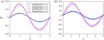
Figure 6 demonstrates the maximum deformation at steady state (
 $h_{max}$
) as a function of Ca; the other parameters are given in the caption. Here, we plot the numerical results along with the deformation until
 $O(\mathit{Ca})$
(i.e.
 $\mathit{Ca}h_{1}$
) as well as
 $O(\mathit{Ca}^{2})$
(i.e.
 $\mathit{Ca}h_{1}+\mathit{Ca}^{2}h_{2}$
). We note that for low values of Ca (
 $\text{until}\approx 0.1$
), the agreement between the numerical and analytical results is near perfect. As we move towards higher values of Ca, the solution until
 $O(\mathit{Ca}^{2})$
is seen to offer greater accuracy. Reasonably good agreement between
 $h_{max}$
from analytical (until
 $O(\mathit{Ca}^{2})$
) and numerical results is observed for
 $\mathit{Ca}\sim 0.2{-}0.25$
, beyond which the error becomes increasingly large. It should be noted that, for all values of Ca, the analytical solutions underestimate the deformation, albeit this is only noticeable for
 $\mathit{Ca}>0.1$
.
The maximum deformation at steady state (
 $h_{max}$
) versus Ca is plotted for
 ${\it\lambda}=1$
,
 $q=2{\rm\pi}/3$
,
 ${\it\theta}=0$
,
 ${\it\varepsilon}=1$
,
 $m=0.2$
and
 $n=0.2$
. We plot the numerical solutions (dots) along with analytical solutions until
 $O(\mathit{Ca})$
(dotted line) and
 $O(\mathit{Ca}^{2})$
(solid line) for comparison. Quite intuitively, for low Ca, the agreement is near perfect, while for higher Ca, the deformation until
 $O(\mathit{Ca}^{2})$
offers a better match with the numerical results.

(a) Plot of the maximum deformation at steady state (
 $h_{max}$
, both analytical and numerical) versus Ca, for
 $q=2{\rm\pi}/3$
and
 $2{\rm\pi}/4$
, with
 ${\it\lambda}=1$
and
 ${\it\varepsilon}=1$
. Good agreement is observed between the two solutions for low Ca. (b) Plot of the maximum deformation at steady state (
 $h_{max}$
, only numerical) versus Ca, for
 ${\it\lambda}=0.1$
, 1 and 10, with
 $q=2{\rm\pi}/3$
and
 ${\it\varepsilon}=1$
. (c) Plot (both analytical solution and numerical results) of the maximum deformation at steady state (
 $h_{max}$
) versus Ca, for
 ${\it\varepsilon}=0.2$
and 2, with
 $q=2{\rm\pi}/3$
and
 ${\it\lambda}=1$
. The other parameters have the following values:
 $m=n=0.2$
,
 ${\it\beta}=1$
,
 ${\it\theta}=0$
and
 $\mathit{Cn}=0.02$
(except for
 $\mathit{Ca}=0.025$
, 0.05 and 0.075, where we have used
 $\mathit{Cn}=0.01$
).

Figure 7(a) depicts the variation in the maximum deformation at steady state as a function of Ca (both analytical and numerical) for two different values of
 $q=2{\rm\pi}/3$
and
 $2{\rm\pi}/4$
; the values of other relevant parameters are given in the caption. The agreement of the analytical results with the numerical ones is good for lower values of Ca (
 ${\sim}0.2$
for
 $q=2{\rm\pi}/3$
and
 $\mathit{Ca}\sim 0.15$
for
 $q=2{\rm\pi}/4$
). However, in the case of
 $q=2{\rm\pi}/4$
, the deformation becomes large (
 ${\sim}0.7$
) for higher capillary numbers, and does not remain in the limit of small deformation, as assumed for the analytical solutions. This figure shows that the magnitude of the deformation increases as the wavelength of modulation is increased, which is in tandem with the conclusions drawn from figure 3(c). As expected, this increase is more pronounced for higher values of Ca. We next move to figure 7(b), where we again plot the maximum deformation at steady state as a function of Ca, this time for three different values of
 ${\it\lambda}=0.1$
, 1 and 10; the values of other relevant parameters are given in the caption. This figure generalizes the results obtained from figure 3(b). An increased viscosity ratio increases the deformation for
 $m<1$
, and as expected this increment is more pronounced for higher values of the capillary number. We observe very large deformations (
 $h_{max}\sim 0.6$
) for
 ${\it\lambda}=10$
at high capillary numbers in this figure. Finally, figure 7(c) depicts the variation in the maximum steady-state deformation with Ca, for two values of permittivity ratio,
 ${\it\varepsilon}=0.2$
and 2; the values of other parameters are given in the caption. This figure is in agreement with figure 4, where we showed that an increment in the permittivity ratio leads to a decrease in the deformation. The same trend is also observed in the present figure. As expected, the change in the deformation is more pronounced for higher values of the capillary number. The analytical and numerical solutions show good agreement for Ca values up to
 ${\sim}0.2$
. The agreement is better for
 ${\it\varepsilon}=2$
, since the deformation is smaller in those cases. This figure (7
a–c) shows that the interface deformation can be augmented as well as suppressed without changing the external parameters, just by adjusting the fluid properties. It is important to note here that although our numerical simulations, in principle, should be valid for large values of
 $h$
, when
 $h$
is very close to 1, our formulation breaks down. It should be noted that here we have assumed the Smoluchowski slip velocity condition at the wall to be valid. The main condition for its validity is that the EDL should be thin compared with the channel height, a condition that is met in most of the microscale flows. However, we must also note the fact that in spite of being thin, the EDL has some finite non-zero thickness. Therefore, for very large values of
 $h$
(for very high deformation), the interface will come very close to the wall and thus can eventually end up inside the EDL. In such cases, the simple Smoluchowski condition will not be valid and one has to analyse the details of charge dynamics and fluid flow inside the EDL as well, starting from the more basic Poisson–Nernst–Planck equations. Although potentially interesting, in the present study we do not actively pursue the aforementioned detailed analysis of the EDL and stick to a simpler Smoluchowski model.
Figure 8 demonstrates the phase plot of the analytical solution for the maximum deformation, as a function of
 ${\it\varepsilon}$
and
 ${\it\lambda}$
; the other parameters are given in the caption. This figure also shows the line of zero or negligible deformation on the
 ${\it\varepsilon}{-}{\it\lambda}$
plane. The variation in
 $h_{max}$
here contains two distinct regions, shown as regions I and II in the figure. In region I, the maximum deformation decreases as we increase
 ${\it\varepsilon}$
, whereas with increase in
 ${\it\lambda}$
it increases. This region corresponds to the variations already shown in figure 7(b,c). However, in region II, this trend reverses, since the deformation (maximum) increases with increase in
 ${\it\varepsilon}$
and decreases when
 ${\it\lambda}$
is increased. These two regions are separated by the line of negligible or zero deformation, where the deformation almost vanishes. Therefore, we conclude that for every choice of viscosity ratio, there is a certain permittivity ratio for which the deformation is completely suppressed. In fact, upon crossing the ‘curve of zero deformation’ the phase of the deformation shifts by 180°, which results in the cusp shown in figure 8. Our numerical results (although not shown here for sake of brevity) also show that for a particular choice of
 ${\it\lambda}$
, one can find a certain permittivity ratio for which the deformation almost vanishes.
Phase plot of the maximum deformation at steady state (from analytical solutions) with the permittivity (
 ${\it\varepsilon}$
) on the
 $x$
axis and the viscosity ratio (
 ${\it\lambda}$
) on the
 $y$
axis. We have also shown the line of minimum
 $h_{max}$
, denoted as ‘curve of zero deformation’. On this line the deformation is negligible, even for higher values of Ca. The rest of the parameters have been chosen as follows:
 $m=n=0.2$
,
 ${\it\beta}=1$
,
 $\mathit{Ca}=0.2$
.

5.2. Transient deformation
In this section, we focus on the variation of the interface deformation with time. It is important to note here that although the interface changes shape with time, the fluid flow always remains quasisteady, as attributable to the approximation
 $\mathit{Oh}^{2}\gg 1$
. The transient evolution of the interface is governed by the equations (3.8), (3.9), (3.17) and (3.19). From these equations it is apparent that the relaxation time (time required to reach steady state) is solely determined by the terms
 $S_{1}$
and
 $S_{3}$
, which are functions of
 ${\it\lambda}$
and
 $q$
. To study the relaxation of the deformed interface, we present the influence of these parameters on the relaxation. Since one of our primary aims is to compare the analytical results for the transience with the numerical results, it is of paramount importance to rescale the time, since the characteristic values used for non-dimensionalizing time in the governing equations are different for the analytical and numerical solutions. To this end, we note that the ratio of the numerical and analytical time scales is Ca. Therefore, comparison between the transience of the two solutions will be possible if the analytical time value (
 $t$
) is multiplied by Ca. In this section all the analytical solutions have been presented by multiplying the corresponding time by Ca.
Variation in the deformation (
 $h$
) with time at an axial location
 $x_{0}=2.2$
, for
 $\mathit{Ca}=0.1$
, 0.2 and 0.3, while the other parameters are as follows:
 ${\it\lambda}=1$
,
 $q=2{\rm\pi}/3$
,
 ${\it\varepsilon}=1$
,
 ${\it\beta}=1$
,
 ${\it\theta}=0$
,
 $m=0.2$
and
 $n=0.2$
. We have plotted both the analytical and numerical results; a reasonable agreement is observed between them. The deformation clearly shows monotonic increment in time, as predicted in § 3.

Figure 9 demonstrates the variation in the deformation at an arbitrarily chosen axial location,
 $x_{0}=2.2$
, with time for three different capillary numbers (0.1, 0.2 and 0.3); the other relevant parameters are given in the caption. We have plotted both analytical results (as given in (3.8)–(3.9) and (3.17)–(3.20)) and the numerical solutions for comparison. As in the previous results, the agreement is reasonably good for lower capillary numbers (
 $\text{until}\sim 0.2$
), while the error is relatively higher for
 $\mathit{Ca}=0.3$
. Both the analytical and numerical results depict similar monotonic variation in time, with roughly equal time scales of variation. The monotonic variation observed in the present figure can be explained from (3.9) and (3.19), which shows that the leading-order deformation, i.e. the most dominant component of the deformation, as well as one of the components from
 $O(\mathit{Ca}^{2})$
(the
 $c_{4}(t)$
term) varies monotonically with time. Therefore, the overall deformation also turns out to be monotonic in time.
Figure 10 depicts the variation in the normalized deformation (analytical as well as numerical) as a function of time, for three different
 ${\it\lambda}=0.1$
, 1 and 10 in (a) and for three different
 $q=2{\rm\pi}/3,2{\rm\pi}/4$
and
 $2{\rm\pi}/5$
in (b); the other parameters are given in the caption. We have normalized the deformation with the corresponding steady-state deformation,
 $h_{\infty }$
. Figure 10(a) is intended to highlight the effects of the viscosity ratio on the time taken by the deformed interface to reach the steady state. To this end, good agreement between numerical and analytical predictions is observed, since the times taken for both are practically equal in figure 10(a). The major point to note from this figure is that the time to reach steady state increases as the viscosity ratio is increased, and this increase in quite drastic for a change of
 ${\it\lambda}$
from 1 to 10. The augmented relaxation time can be attributed to the fact that higher viscosity will result in slower motion of both the fluids, which will eventually lead to a slower deformation rate. This is manifested as a larger relaxation time for interface deformation. In addition to this, increased
 ${\it\lambda}$
also leads to increased asymmetry in the flow for
 $m<1$
. This leads to larger deformation, which eventually causes the total deformation time to increase. It is interesting to note that both the magnitude of the deformation as well as the time taken to reach the steady state are larger for larger
 ${\it\lambda}$
. On the other hand, with increase in the modulation wavelength (decrease in
 $q$
), there is a significant increase in the time required to reach steady state. This can be attributed to the fact that as we increase the modulation wavelength, the deformation tends to increase, as shown in figures 3(c) and 7(a). Thus, with all other parameters (especially the viscosity) kept constant, the interface is naturally expected to take more time to reach steady state, simply because it has to deform more. In this case also the asymptotic theory agrees well with the numerical simulation results.
The normalized deformation (normalized with the steady-state deformation,
 $h_{\infty }$
) as a function of time is plotted at an axial location of
 $x_{0}=2.2$
(a) and
 $x_{0}=2.5$
(b): (a) for three different
 ${\it\lambda}=0.1$
, 1 and 10, with
 $\mathit{Ca}=0.1$
,
 $q=2{\rm\pi}/3$
and
 $m=n=0.2$
; (b) for three different
 $q=2{\rm\pi}/3$
,
 $2{\rm\pi}/4$
and
 $2{\rm\pi}/5$
, with
 $\mathit{Ca}=0.05$
,
 ${\it\lambda}=1$
and
 $m=n=0.2$
. The other parameters were taken as
 ${\it\varepsilon}=1$
,
 ${\it\theta}=0$
,
 ${\it\beta}=1$
. We plot both analytical and numerical solutions and good agreement is observed between the two. This plot is intended to demonstrate the effects of viscosity and modulation wavelength on the time taken to reach the steady state. It is important to note that the analytical and numerical values have been normalized with their respective steady-state deformations.

(a1,a2) Contours of the steady-state streamlines depicting the flow path, for
 $\mathit{Ca}=0.1$
,
 ${\it\lambda}=1$
,
 $m=n=0.2$
,
 $q=2{\rm\pi}/3$
, and the interface, as shown by the thick line. (b1,b2) Contours of the steady-state streamlines depicting the flow path, for
 $\mathit{Ca}=0.2$
,
 ${\it\lambda}=2$
,
 $m=n=0.2$
,
 $q=2{\rm\pi}/3$
, and the interface, as shown by the thick line. In both the figures, (1) is from the numerical solution, whereas (2) shows the analytical solution. Reasonably good agreement is observed between the analytical and numerical solutions in both the cases. The other parameters are:
 ${\it\beta}=1$
,
 ${\it\epsilon}=1$
and
 ${\it\theta}=0$
.

5.3. Flow dynamics
In this section we discuss the nature of the flow for the combination of parameters presented in the previous two sections. We start with figure 11(a,b), where the contours of the steady-state streamlines are shown as obtained from numerical (figure 11
a1,b1) and analytical (figure 11
a2,b2) results; the relevant parameters are given in the caption. We also show the location of the deformed interface (thick line) to differentiate the streamlines of the two fluids. Analytical solutions for the streamlines are given in (3.7) and (3.16), while the streamlines from the numerical solutions are calculated from the relation
 $\text{d}{\it\psi}=u\,\text{d}y-v\,\text{d}x$
, where it has been assumed that for the numerical solutions
 ${\it\psi}=0$
at the bottom wall. In both the cases the agreement between the numerical and analytical solutions is reasonable. Several interesting points can be noted from the present figure. First, recirculation rolls are present in both the fluids, which are attributable to the axially modulated potential on the wall. The axially invariant part of the potential contributes to the wavy but non-recirculating streamlines, leading to a net throughput. The waviness in these streamlines is, of course, an outcome of the presence of an axially modulated surface potential. A second and the most interesting point to note is the effect of the deformation on the shape of the streamlines. It can be observed that the deformation distorts all the streamlines, including the recirculation rolls, since they tend to be parallel to the interface at steady state. This distortion is, of course, more pronounced for the case of
 $\mathit{Ca}=0.2$
and
 ${\it\lambda}=2$
in figure 11(b1,b2), since the deformation is higher for this combination of parameters.
Figure 12 (values of relevant parameters are given in the caption) embodies an extreme case of the distortion of streamlines, as reported in the preceding figures. It can be observed that the deformation is very large (maximum deformation
 ${\sim}0.7$
), which distorts all the streamlines extremely to make them parallel to the interface at steady state. Here, we have only shown the numerically obtained streamlines, since the approximate analytical solutions are not expected to hold for such high deformation magnitudes.
Contours of the steady-state streamlines (only numerical solutions) for large interface deformation, with
 $\mathit{Ca}=0.3$
,
 ${\it\lambda}=1$
,
 $m=n=0.2$
,
 ${\it\varepsilon}=1$
,
 ${\it\beta}=1$
,
 ${\it\theta}=0$
and
 $q=2{\rm\pi}/4$
. The location of the interface has also been plotted (thick line). This figure demonstrates an extreme case of deformation and streamline distortion.

(a,b) Contours of the steady-state streamlines for
 $\mathit{Ca}=0.1$
,
 ${\it\lambda}=1$
,
 $q=2{\rm\pi}/3$
,
 ${\it\varepsilon}=1$
,
 ${\it\beta}=1$
,
 ${\it\theta}=0$
,
 $m=-0.2$
and
 $n=0$
. The location of the interface has been shown with a thick line. Panel (a) demonstrates the results obtained from numerical solutions, whereas (b) is from the analytical solution. (c) Plot of the steady-state deformation for two different values of
 $m=0.2$
(curve with lower amplitude) and
 $-0.2$
(curve with larger amplitude), while the other parameters are the same as in (a) and (b). We have plotted both numerical (circles) and analytical (lines) solutions, and the agreement between them is reasonably good.

We next investigate a special case in figure 13(a–c), where we depict the contours of the streamlines for
 $m=-0.2$
and
 $n=0$
(both analytical (figure 13
a) and numerical (figure 13
b)), which indicates that the potentials at the top and the bottom walls are out of phase (values of other relevant parameters are given in the caption). Good agreement is observed between the analytical and numerical results. It is interesting to note that in the present case two recirculation rolls appear in the top fluid, whereas for cases with
 $m>0$
, reported in the preceding figures, only one roll exists in the top fluid. This can be attributed to the fact that for
 $m<0$
the fluid on top tries to move in the opposite direction to the bottom fluid, whereas the bottom fluid tries to drag the top fluid with itself. Since
 $m=0.2$
, the slip velocity in the top fluid is weak, and hence the part of this fluid residing close to the interface feels more drag due to the bottom fluid (note that
 ${\it\lambda}=1$
) compared with the electro-osmotic forcing due to Smoluchowski slip. Therefore, this part of the fluid tends to move along the direction of the bottom fluid, whereas the part near the top wall moves in the opposite direction. This mismatch in the direction of movement gives rise to multiple rolls in the fluid on top. Finally, we note that the deformation of the interface (at steady state) for
 $m=-0.2$
has a greater magnitude than that for
 $m=0.2$
(i.e.
 $m>0$
), as shown in figure 13(c), where the steady-state deformation has been plotted keeping the parameter values the same as in (a) and (b), only altering
 $m$
between
 $-0.2$
and 0.2. This can be explained very easily based on the argument of asymmetry, mentioned in the explanation of figure 3(b). Clearly,
 $m=-0.2$
signifies more asymmetry, and since the deformation is primarily caused here by asymmetry, it leads to a higher amount of deformation.
Following figure 13, we now attempt to show the deformation and the resulting flow structures for the intermediate phase shift angles (
 ${\it\theta}$
) as depicted in figure 14(a–c) (only numerical results). Figure 14(a) demonstrates the variation in the interface deformation
 $(h_{\infty })$
at steady state, for five different choices of
 ${\it\theta}=0$
,
 ${\rm\pi}/4$
,
 ${\rm\pi}/2$
,
 $3{\rm\pi}/4$
and
 ${\rm\pi}$
; the values of the rest of the parameters are given in the caption. We note that as the phase shift angle increases, the deformation increases, reaching a maximum at
 ${\it\theta}={\rm\pi}$
. This can again be explained from the arguments of asymmetry, since increasing
 ${\it\theta}$
leads to increased asymmetry between the two halves of the channel, which in turn causes the interface to deform more. Finally, in figure 14(b,c) we show the streamlines for two choices of
 ${\it\theta}={\rm\pi}/2$
and
 ${\rm\pi}$
. We can see that the only notable effect of
 ${\it\theta}$
here is that the position of the recirculation rolls in the upper fluid (fluid 1) changes and tends to shift to the left as
 ${\it\theta}$
is increased. At the same time, the roll in fluid 2 tends to get distorted as
 ${\it\theta}$
is increased.
(a) Plot (only numerical results) of the steady-state deformation
 $(h_{\infty })$
versus
 $x$
, for five different values of the phase shift angle,
 ${\it\theta}=0$
,
 ${\rm\pi}/4$
,
 ${\rm\pi}/2$
,
 $3{\rm\pi}/4$
and
 ${\rm\pi}$
. (b,c) Contours of the steady-state streamlines (only numerical results) depicting the flow path, for two different values of the phase shift angle, (b)
 ${\it\theta}={\rm\pi}/2$
and (c)
 ${\it\theta}={\rm\pi}$
. The other parameters have the following values:
 $m=2$
,
 $n=0.2$
,
 ${\it\lambda}=0.5$
,
 $q=2{\rm\pi}/3$
,
 ${\it\beta}=1$
,
 ${\it\varepsilon}=1$
,
 $\mathit{Ca}=0.1$
and
 $\mathit{Cn}=0.02$
. The interface is represented by the red line.

We acknowledge that more parametric studies, apart from those presented here, can be executed depicting the resulting streamline and deformation patterns. However, we strongly feel that the parametric studies reported herein are sufficient to highlight the essential features of flow dynamics and deformation patterns, within the assumptions of the present framework. Therefore, we restrain ourselves from performing any more such studies and conclude the present analysis.
6. Conclusions
The electro-osmotic flow of two superimposed fluids in the presence of a modulated surface charge, under the thin-EDL limit, has been investigated in the present analysis. We have calculated the velocity fields and the corresponding deformations analytically through domain perturbations for small values of Ca, whereas numerical simulations have also been performed for arbitrary values of Ca and large deformation. We extended our asymptotic methods to calculate the velocity fields until
 $O(\mathit{Ca})$
and the deformation until
 $O(\mathit{Ca}^{2})$
. The analytical and numerical results for the deformation and flow patterns showed reasonably good agreement for low capillary numbers (
 ${\sim}0.2$
). In the analytical solutions, inertial effects have been neglected, as they are attributable to low values of Re and large values of
 $\mathit{Oh}^{2}$
. However, the numerical simulations have been performed including the inertial effects for a more general analysis.
Several interesting conclusions can be drawn from the present analysis. We have successfully demonstrated that for low values of Ca the deformation exhibits simple sinusoidal behaviour, whereas for large deformations more complex variation with the axial coordinate is shown. Our analysis shows that the interface deformation can be either suppressed or augmented depending on the fluid properties, without changing the external parameters. For example, we show that an increase in the viscosity ratio (as defined for the present problem) results in an increase in the deformation, on account of increased asymmetry, whereas increase in the permittivity ratio leads to a decrease in the deformation, for
 $0<m<1$
. We have further shown that an increase in the modulation wavelength results in significant augmentation in the deformation of the interface. However, it is important to note that the present analysis assumes
 $d/H\sim O(1)$
(
 $d$
is the wavelength of modulation). Therefore, any general conclusion regarding the effects of
 $d$
on the deformation for larger values cannot be made from the present analysis. A very interesting conclusion of the present analysis is that, even for very small values of the capillary number, a fairly large amount of deformation can be realized, with proper choices of fluid properties and geometric parameters. Therefore, when analysing the flow in such cases, one cannot neglect the deformation and assume the interface to be flat on account of low values of Ca. We have also explored the nature of the flow by visualizing the streamlines. Our results reveal that the streamlines at steady state are distorted by the deformation, since they have to be parallel to the interface.
It is possible to make several future extensions and improvements to the present analysis. For example, a possible and potentially interesting extension is a stability analysis of the flow described in the present system. In addition to this, the effects of the presence of surface-active agents on the deformation and flow dynamics can also lead to very interesting results. Finally, it might be extremely helpful to look into the electro-osmosis of superimposed fluids when the fluids are non-Newtonian in nature, since the use of non-Newtonian fluids in microscale flows is abundant in practice (Brust et al. Reference Brust, Schaefer, Doerr, Pan, Garcia, Arratia and Wagner2013; Dhar, Ghosh & Chakraborty Reference Dhar, Ghosh and Chakraborty2014) due to their importance in biological systems.
Acknowledgements
The corresponding author gratefully acknowledges the financial support provided by SRIC, IIT Kharagpur under the Project ‘Centre of Excellence for Training and Research in Microfluidics’.
Appendix A. Expressions for the constants in analytic solutions
The leading-order deformation as expressed in (3.9) is given by
 $$\begin{eqnarray}h_{1}(x,t)=c_{1}(t)\sin (qx);\quad c_{1}(t)=S_{2}(q,{\it\lambda},m,{\it\varepsilon})(1-\text{e}^{-t/S_{1}({\it\lambda},q)}).\end{eqnarray}$$
In (A 1),
 $S_{2}$
is given by
 $$\begin{eqnarray}\left.\begin{array}{@{}c@{}}\displaystyle S_{2}=\frac{A_{1}\cosh (3q)+A_{2}\cosh (q)+A_{3}\sinh (q)}{({\it\lambda}+1)(\sinh ^{2}(q)-q^{2})(\sinh (q)\cosh (q)-q)},\\ \text{where }\displaystyle A_{1}={\textstyle \frac{1}{2}}({\it\lambda}+1)({\it\varepsilon}m-1),\\ \displaystyle A_{2}={\it\varepsilon}m\left[2q^{2}(1-{\it\lambda})-{\textstyle \frac{1}{2}}({\it\lambda}+1)\right]+\left[2q^{2}(1-{\it\lambda}){\textstyle \frac{1}{2}}({\it\lambda}+1)\right],\\ \displaystyle A_{3}=4q({\it\lambda}-{\it\varepsilon}m).\end{array}\right\}\end{eqnarray}$$
On the other hand,
 $S_{1}$
and
 $S_{3}$
are expressed as
 $$\begin{eqnarray}\displaystyle & \displaystyle S_{1}=\frac{{\textstyle \frac{1}{4}}({\it\lambda}+1)^{2}\cosh (4q)-({\it\lambda}+1)^{2}\left(2q^{2}+{\textstyle \frac{1}{4}}\right)-2q^{4}({\it\lambda}-1)^{2}}{q({\it\lambda}+1)(\sinh ^{2}(q)-q^{2})(\sinh (q)\cosh (q)-q)}, & \displaystyle\end{eqnarray}$$
 $$\begin{eqnarray}\displaystyle & \displaystyle S_{3}=\frac{{\textstyle \frac{1}{8}}({\it\lambda}+1)^{2}\cosh (8q)-({\it\lambda}+1)^{2}\left(4q^{2}+{\textstyle \frac{1}{8}}\right)-16q^{4}({\it\lambda}-1)^{2}}{q({\it\lambda}+1)(\sinh ^{2}(2q)-4q^{2})(\sinh (2q)\cosh (2q)-2q)}. & \displaystyle\end{eqnarray}$$
 $a_{1}^{(0)},b_{1}^{(0)},\dots ,$
etc. have the following form:
 $$\begin{eqnarray}\left.\begin{array}{@{}c@{}}\displaystyle a_{1}^{(0)}=b_{1}^{(0)}=\frac{1}{q}\frac{\text{d}c_{1}}{\text{d}t},\\ \displaystyle a_{k}^{(0)}=M_{k}^{(0)}({\it\lambda},q)\frac{\text{d}c_{1}}{\text{d}t}+N_{k}^{(0)}({\it\lambda},q,{\it\varepsilon},m),\\ \displaystyle b_{k}^{(0)}=P_{k}^{(0)}({\it\lambda},q)\frac{\text{d}c_{1}}{\text{d}t}+Q_{k}^{(0)}({\it\lambda},q,{\it\varepsilon},m),\end{array}\right\}\end{eqnarray}$$
for
 $k=2,3,4$
. On the other hand, the rest of the constants can be expressed in the following form:
 $$\begin{eqnarray}\left.\begin{array}{@{}c@{}}\displaystyle a_{1}^{(1)}=-\frac{1}{2q}qc_{1}(a_{2}^{(0)}+qa_{3}^{(0)})-\frac{1}{2q}\frac{\text{d}c_{2}}{\text{d}t},\\ \displaystyle b_{1}^{(1)}=-\frac{1}{2q}qc_{1}(b_{2}^{(0)}+qb_{3}^{(0)})-\frac{1}{2q}\frac{\text{d}c_{2}}{\text{d}t},\\ \displaystyle a_{i}^{(1)}=M_{i}^{(1)}({\it\lambda},q)\frac{\text{d}c_{2}}{\text{d}t}+\,N_{i}^{(1)}({\it\lambda},q,{\it\varepsilon},m,t)c_{1},\\ \displaystyle b_{i}^{(1)}=P_{i}^{(1)}({\it\lambda},q)\frac{\text{d}c_{2}}{\text{d}t}+Q_{i}^{(1)}({\it\lambda},q,{\it\varepsilon},m,t)c_{1},\\ \displaystyle k_{1}=l_{1}=-\frac{1}{q}\frac{\text{d}c_{4}}{\text{d}t}+\frac{n({\it\varepsilon}m+1)}{{\it\lambda}+1}c_{1},\\ \displaystyle k_{i}=\hat{M}_{i}^{(1)}\frac{\text{d}c_{4}}{\text{d}t}+\hat{N}_{i}^{(1)}c_{1},\quad l_{i}=\hat{P}_{i}^{(1)}\frac{\text{d}c_{4}}{\text{d}t}+\hat{Q}_{i}^{(1)}c_{1},\quad i=2,3,4.\end{array}\right\}\end{eqnarray}$$
The terms,
 $M$
,
 $N$
,
 $P$
,
 $Q$
, etc. are functions of
 ${\it\lambda}$
,
 $q$
,
 $m$
, etc., with complicated algebraic expressions. In particular, the terms
 $N_{i}^{(1)}$
are of the following form:
 $N_{i}^{(1)}=T_{i}({\it\lambda},q,{\it\varepsilon},m)(\text{d}c_{1}/\text{d}t)+\tilde{T}_{i}({\it\lambda},q,{\it\varepsilon},m)$
. We do not explicitly mention the detailed expressions of the constants here. As mentioned in § 3, the MATLAB and MAPLE files containing these expressions can be made available upon request. Since deformations at
 $O(\mathit{Ca})$
also have similar expressions to those given in (A 1), we do not explicitly mention them here.
Appendix B. Effect of inertia on deformation and flow
In this appendix, the effects of inertia on the interface deformation and flow dynamics are discussed. To this end, we solve (4.9a
)–(4.9e
) subject to (4.9f
) and (4.10a
)–(4.10d
). Figure 15(a,b) depicts the effect of inertia on the interface deformation for five different values of Re; the values of the other parameters are given in the caption. In figure 15(a), we show the variation in the normalized deformation (normalized w.r.t. the steady-state deformation) as a function of time at an axial location of
 $x_{0}=2.2$
, while figure 15(b) depicts the actual deformation at the same axial location for the same set of parameters. It is very interesting to note that the Reynolds number has a negligible effect on both the deformation time and the steady-state deformation height, even for Re as large as
 $O(1)$
. However, a closer look at the figure indicates that the deformation lags slightly behind in time as the inertia increases. The inset in figure 15(b) reveals that the steady-state deformation increases slightly as the value of Re is increased.
(a) The normalized deformation (normalized with the steady-state deformation,
 $h_{\infty }$
) as a function of time is plotted at an axial location of
 $x_{0}=2.2$
for different values of
 $\mathit{Re}=0.001$
, 0.01, 0.1, 0.5 and 1. (b) The actual deformation at the same location for identical values of Re. Inset: zoomed-in variation in the deformation for
 $t=3{-}4$
. The other parameters have the following values:
 $m=n=0.2$
,
 ${\it\lambda}=1$
,
 $q=2{\rm\pi}/3$
,
 ${\it\beta}=1$
,
 ${\it\epsilon}=1$
,
 $\mathit{Ca}=0.2$
and
 $\mathit{Cn}=0.02$
.