





1. Introduction
Aerodynamic interactions between multiple lifting bodies are ubiquitous in both engineered and natural systems. When two wings, blades or lifting surfaces move in proximity (particularly when they translate in opposite directions), each generates a time-dependent velocity and pressure field that alters the other’s effective incidence, producing a coupled and transient aerodynamic environment. Such mutual interference governs performance and unsteady loading in systems ranging from multi-rotor aircraft and wind-turbine arrays to high-speed trains and biological flight. However, despite its prevalence, the underlying fluid mechanics of these interactions remain incompletely characterised, particularly during transient encounters.
In engineered systems, such aerodynamic interference manifests itself in various forms. Multi-body configurations that exhibit such interference include counter-rotating coaxial rotors (Lakshminarayan & Baeder Reference Lakshminarayan and Baeder2009; Singh et al. Reference Singh, Kang, Cameron and Sirohi2016; Cameron et al. Reference Cameron, Sirohi, Feil and Rauleder2017; Singh & Friedmann Reference Singh and Friedmann2017; Uehara et al. Reference Uehara, Sirohi, Feil and Rauleder2019), vertical-axis wind turbine arrays (Rajagopalan et al. Reference Rajagopalan, Rickerl and Klimas1990; Ahmadi-Baloutaki et al. Reference Ahmadi-Baloutaki, Carriveau and Ting2016) and flapping-wing systems operating at close phase spacing. In counter-rotating coaxial rotors, the periodic cross-over of blades generates transient loading and noise excursions, yet most prior analyses have focused on performance rather than the underlying unsteady mechanisms (Singh & Friedmann Reference Singh and Friedmann2017; Schatzman et al. Reference Schatzman, Komerath and Romander2017). Viscous-vortex-particle simulations by Singh & Friedmann (Reference Singh and Friedmann2017) and Navier–Stokes computations by Schatzman et al. (Reference Schatzman, Komerath and Romander2017) revealed qualitative similarities in the lift history during cross-over, but disagreed on phase and magnitude even for non-lifting (
 $\alpha = 0^\circ$
) configurations. These discrepancies point to an incomplete physical understanding of instantaneous flow coupling, particularly the role of induced velocities, pressure redistribution and finite-thickness effects. Comparable interference effects occur in bluff-body cross-overs such as high-speed train encounters, where a transient low-pressure region forms between approaching bodies (Ogawa & Fujii Reference Ogawa and Fujii1993), suggesting that thickness-induced potential flow interactions may play a dominant role even in streamlined lifting flows. These examples share a common theme: the unsteady flow around each body is not isolated, but mutually driven by the motion and induced field of its neighbour.
Similar interference mechanisms appear in nature, often exploited for flight control or energetic benefit. Dragonflies, for example, flap fore and hind wings that are separated by approximately one wing width, and the wings often cross near midstroke with phase differences tuned to the flight mode (Thomas et al. Reference Thomas, Taylor, Srygley, Nudds and Bomphrey2004; Wang Reference Wang2008). During these cross-overs, the fore wing experiences the induced upwash generated by the hind wing and vice versa, leading to modulated lift, drag and power expenditure. Out-of-phase motion can reduce aerodynamic power requirements, whereas in-phase beating enhances thrust. Similar phenomena occur in hovering birds such as hummingbirds, whose wings re-encounter their own or neighbouring wakes (Warrick et al. Reference Warrick, Tobalske and Powers2005; Altshuler et al. Reference Altshuler, Princevac, Pan and Lozano2009). Thus, these biological systems exemplify natural instances of wing–wing interference, where wings concurrently create and react to each other’s induced fields. These examples further highlight the universality of mutual aerodynamic induction and motivate its study in a controlled canonical configuration.
The analytical foundation for interpreting such interactions lies in classical unsteady aerodynamic theories developed for externally imposed disturbances. Theodorsen’s function (Theodorsen Reference Theodorsen1934) describes harmonic aerofoil motion, Kussner’s function (Küssner Reference Küssner1936; Küssner & Jones Reference Küssner and Jones1960) models a stationary sharp-edge gust and Miles’s formulation (Miles Reference Miles1956) generalises to a travelling gust with finite convective velocity. These indicial responses separate the lift into non-circulatory and circulatory components, facilitating refined linear predictions of gust-response dynamics. In such problems, the imposed gust modifies the local inflow seen by the aerofoil, thereby altering its instantaneous effective angle of attack and unsteady force response. However, they all assume that the perturbation field is externally defined and unaffected by the aerofoil itself. Loewy (Reference Loewy1957) later extended this framework to include a returning wake, introducing partial feedback between the aerofoil and its shed vorticity. This concept of wake–body coupling represents an intermediate step between externally forced and mutually induced interactions.
During wing cross-over, an analogous mechanism arises: the induced velocity field generated by one wing modifies the local inflow experienced by the other wing, producing transient changes in effective incidence and aerodynamic loading in a manner conceptually similar to a convecting gust encounter. However, when two bodies move relative to each other, each simultaneously generates and responds to the disturbance field of the other, creating a self-induced gust problem that has no direct analogue in existing linear theory. Here, ‘self-induced gust’ refers to the transient disturbance field generated by the interaction of the two bodies, indicating a mutual induction at the system level rather than that of a single body.
Although a complete theoretical framework for such cross-over interactions remains lacking, the observed similarities between classical gust-response problems and cross-over load histories suggest that existing linear theories may still provide useful physical insight when carefully interpreted. In both cases, an unsteady induced velocity field modifies the instantaneous inflow to the lifting surface and thereby governs the transient lift response. For gust encounters, this disturbance is externally prescribed, whereas in the cross-over problem, it is generated by the neighbouring moving wing. Nevertheless, the resulting force dynamics may exhibit comparable signatures, including phase-lagged circulatory growth, non-circulatory loading peaks and sensitivity to disturbance convection speed. Existing linear theories, therefore, offer a useful means of examining the relative importance of circulatory loading, added-mass effects and convecting induced disturbances during close-passage encounters. The extent to which these models remain applicable is expected to depend on nonlinear effects such as strong flow separation and vortex interaction (Zaide & Raveh Reference Zaide and Raveh2006; Corkery & Babinsky Reference Corkery and Babinsky2019; Andreu-Angulo et al. Reference Andreu-Angulo, Babinsky, Biler, Sedky and Jones2020; Biler et al. Reference Biler, Sedky, Jones, Saritas and Cetiner2021).
The primary objective of the present study is therefore to elucidate the underlying aerodynamic mechanisms governing the cross-over of two counter-translating wings in close proximity through combined experimental measurements and analytical interpretation. Consequently, the present work employs established linear unsteady aerodynamic formulations as physics-based diagnostic tools to interpret the measured force response, assess their applicability to cross-over motions, and distinguish the relative roles of circulatory and non-circulatory loading. Time-resolved force and flow-field measurements are used to identify the governing trends associated with induced velocity, gap-pressure interaction and circulation development during cross-over. The experiments systematically vary wing pitch, spacing and geometry to determine the dominant non-dimensional parameters controlling the response. These findings provide a physical foundation for future development of improved predictive models for interacting lifting surfaces undergoing cross-over manoeuvres.
The remainder of the paper is organised as follows. The experimental facility, the aerofoil configuration and the instrumentation are described in § 2. Characterisation and validation of the facility are presented in § 3. Section 4.1 discusses the measured aerodynamic loading and the evolution of the associated flow field during cross-over. The induced velocity field is modelled as a moving gust and analysed using the Miles and Kussner frameworks in § 4.2. Finally, the influence of key non-dimensional parameters on cross-over dynamics is discussed in § 4.3 and the main conclusions are summarised in § 5.
2. Methodology
2.1. Experimental facility
The experiments for the current study were carried out in a hydrodynamic towing tank facility. The set-up was built on top of an existing water tank in the Department of Aerospace Engineering at Auburn University. The tank has dimensions of
 $2.4 \times 0.6 \times 0.6\,\text{m}$
. Two identical linear traverses, each with an actuation length of
 $1\ \text{m}$
, were positioned on top of the towing tank to enable the translation of the lifting bodies. These linear traverses were mechanically connected using a bevel gear arrangement. The actuation was achieved using a single AC servo motor (ECMA-C20807RS), as illustrated in figure 1. This motor has a power rating of
 $750\ \text{W}$
, with speed and torque ratings of
 $3000\,\text{rpm}$
and
 $2.39\ \text{N m}$
, respectively. The pitch of the linear traverse was
 $95\ \text{mm}$
per motor rotation and the maximum speed of the facility was limited to
 $1.2\ \text{m s}^{-1}$
, according to the specifications provided by the manufacturer.
The AC servo motor was controlled using a servo motor controller (Delta ASD-B2-0721-B). The servo motor and the controller were placed on a common electric ground and an electromagnetic interference (EMI) filter was embedded in the power circuit to reduce electromagnetic interference on the instrumentation. Additionally, a skim plate, similar to that reported in the previous literature (Stevens et al. Reference Stevens2016), was placed on the surface of the water to reduce the effects of surface waves produced during the translation of wings. A bottom plate was also placed to simulate infinite wing conditions by reducing the tip effects. The spacing between the wing tip and the bottom surface was less than
 $2\,\text{mm}$
(Fuglsang et al. Reference Fuglsang, Antoniou, Sørensen and Madsen1998). Prior to the cross-over study, this facility was validated through single-wing translation experiments.
CAD representation of the hydrodynamic towing tank facility to study wing cross-over. The high-speed laser and two side-by-side cameras facilitate two-dimensional (2-D) particle image velocimetry (PIV) measurements over a large field of view. Graphical representation of the spatial nomenclature used for the study is shown on the right.

Figure 1. Long description
Panel A: A CAD representation of the hydrodynamic towing tank facility. The setup includes a motor, bevel gear, linear actuators, top and bottom plates, wing assembly, torque sensor, adapters, a 3-axis load cell, high-speed cameras, and a laser sheet. The wings are positioned side by side, and the high-speed cameras are placed below the setup. Panel B: A graphical representation of the spatial nomenclature used for the study. It shows the chord (c), translation plane, wing spacing (d/c), and the relative positions of Wing 1 and Wing 2. The diagram indicates the direction of wing movement and the alignment of the quarter chord location.
2.2. Instrumentation
The wings were attached to the linear translation stage through an interface that housed multi-axis loadcells for measuring the wing loads, namely lift, drag and pitching moment. Lift and drag were measured using a multi-axis force transducer calibrated to
 $10\ \text{N}$
. Similarly, the pitching moment was measured using a single-axis moment sensor calibrated to
 $0.12\ \text{N m}$
. These loadcells had a sensitivity of
 $0.2\ \text{mV V}^{-1}$
. The loadcells were connected to amplifiers (Tacuna EMBSGB200), which filtered and converted the millivolt signal into a
 $(0{-}5)\ \text{V}$
output range. The amplifiers had a low-pass filter with a corner frequency of
 $1000\ \text{Hz}$
. The force measurements’ spectral analysis showed that the facility’s inherent vibrations were mostly above
 $40\ \text{Hz}$
. Therefore, a digital low-pass filter of
 $40\ \text{Hz}$
was applied to all the data presented here. The loadcell measurements were synchronised with the measurement from an internal 17-bit encoder in the motor, which provided real-time positional information of the wings during the translation. The signal from this encoder had high-frequency noise due to EMI; thus, it was filtered using a first-order RC low-pass filter. The loadcell data were acquired through an NI-9239 analogue input module connected to an NI cDAQ-9174, while the encoder data were acquired through an NI-9401 digital module connected to the same chassis.
The uncertainty in the force measurements arises from sources like sensor calibration and resolution, run-to-run repeatability, and signal processing. The multi-axis force transducer and moment sensor contribute a calibration uncertainty of approximately
 $\pm 0.1\,\,\%$
of full scale, based on manufacturer specifications and pre-experiment calibration procedures. Run-to-run repeatability, assessed through repeated measurements under identical operating conditions, yielded standard deviations of
 ${\leqslant} 3\,\%$
of the peak loads, primarily due to small variations in wing alignment and manufacturing uncertainties. Signal processing introduced negligible additional uncertainty, as the 40 Hz digital low-pass filter was selected to remove facility-induced vibrations (
 ${\gt}40$
Hz) while preserving the dominant unsteady loading content.
2.3. Flow measurements
The wing flowfield was measured using time-resolved particle image velocimetry (PIV). Illumination was achieved using a dual-head Nd:YLF laser (527nm wavelength and
 $30\,\text{mJ pulse}^{-1}$
at
 $1\,\text{kHz}$
). The laser sheet was parallel to the translation direction and the cameras were placed below the towing tank, as shown in figure 1. VEO 640L high-speed cameras, which capture the images at
 $1400\,\text{fps}$
at
 $2560\times 1600$
pixels, were used to capture the flowfield images. These cameras were placed side-by-side to maximise the field of view (FOV). A fixed focal length lens with
 $50\,\text{mm}$
focal length and an aperture setting of
 $f/1.8$
was used for each camera. Each camera covered a FOV of
 $(10.4\times 6.5)c$
(where
 $c$
= wing chord length) and with an overlap of
 $14\,\%$
between the FOV of the two cameras, the resultant FOV was
 $(18.2\times 6.5)c$
. The calibration for PIV measurements was carried out simultaneously for both cameras with the same calibration plate that covered the entire field of view. The magnification and calibration factors for the current experiments were
 $0.068$
and
 $6.85\,\text{pixel (mm)}^{-1}$
, respectively. The reprojection error for the calibration process using the custom calibration plate was
 ${\leqslant} 0.4$
pixel.
The current study used polyamide spheres with a mean particle diameter of
 $55\,{\unicode[Arial]{x03BC}}\text{m}$
as seeding particles. The raw PIV images were acquired and processed using DaVis 10.2. The flowfield data were acquired at
 $400\,\text{Hz}$
in time-series mode. The velocity fields were then obtained by processing the images using the multi-grid, multi-pass sliding sum-of-correlation cross-correlation technique with an initial and final interrogation window of size
 $64\times 64$
pixels and
 $24\times 24$
pixels, respectively, each with an overlap of 50 %. The filter length for the sliding sum-of-correlation was set to 4. The vector fields were post-processed to remove spurious vectors. The vector fields were then stitched together to obtain the final flowfield with a
 $1.75\,\text{mm}$
(
 $0.048\,c$
) vector spacing resolution. The uncertainties in the velocity measurements were quantified using the correlation statistics method (Wieneke Reference Wieneke2015), where the uncertainty is proportional to the residual positional disparity between the matched correlation peaks (Sciacchitano Reference Sciacchitano2019). The resulting uncertainty in the velocity across the flowfield for all cases was
 ${\leqslant} 1\,\%$
of the average velocity in the flow field.
2.4. Operating conditions
First, the facility was characterised using NACA0012 aerofoil wings, which were accelerated to a steady state. Here, the effect of acceleration distance and Reynolds number (
 ${\textit{Re}}=cU_\infty /\nu$
, where
 $U_\infty$
is the steady translation speed) on the load characteristics was quantified. Initially, the acceleration distance was varied (refer to table 1) by keeping
 ${\textit{Re}}$
fixed at
 $25\,000$
. Similarly, the wing was held at a constant pitch angle,
 $\alpha = 6^\circ$
, and accelerated to a steady state by varying the Reynolds number to understand the effect of
 ${\textit{Re}}$
. Then, the steady-state characteristics of each wing were assessed by placing it on both translation stages. This arrangement was used to quantify the potential differences between the wings and the translation stages. Here, the pitch angle of the wings was changed from
 $0^\circ$
to
 $14^\circ$
at an increment of
 $2^\circ$
, and the lift, drag and moment experienced by the wings were measured.
Summary of the operating conditions for facility characterisation.

Table 1. Long description
A table with one row and four columns summarizing test conditions for facility characterization. The columns are labeled Test conditions, Pitch angle (α), Reynolds number (Re), and Acceleration distance (s_a/c). The row under Test conditions states Acceleration to steady state. The Pitch angle (α) column lists angles 0°, 2°, 4°, 6°, 8°, 10°, 12°, 14°. The Reynolds number (Re) column lists values 15000, 25000, 35000. The Acceleration distance (s_a/c) column lists values 1, 2, 4, 8.
The cross-over experiments were then carried out for flat plates and wings with NACA0012 and NACA0018 aerofoil profile sections. The two wings under investigation were called Wing 1 and Wing 2. Wing 1 occupied the lower position, while Wing 2 was above it. Both wings had a span of
 $0.254$
metres. The chord length was varied for the NACA0012 profile wing sections as
 $c = 0.036\,\text{m}$
and
 $c = 0.072\,\text{m}$
, resulting in the aspect ratios of
 $AR = 7$
and
 $AR = 3.5$
, respectively. For the wing with a smaller chord length, experiments were carried out at translation speeds in the range of
 $U_\infty = (0.41{-}0.97)\,\text{m s}^{-1}$
, at pitch angles in the range of
 $\alpha = 0^\circ {-} 14^\circ$
and wing spacing in the range (refer to figure 1) of
 $d/c = 1.4{-}3$
. Flowfield measurements were also carried out for some of the specific cases. For wings with larger chord lengths of
 $c = 0.072\,\text{m}$
, experiments were carried out at a fixed wing spacing of
 $d/c = 1.4$
and a pitch angle of
 $\alpha = 0^\circ$
. The translation speed was varied as
 $U_\infty = (0.209{-}0.69)\,\text{m s}^{-1}$
. For flat plates and wings with NACA0018 aerofoil profile, the experiments were carried out at a pitch angle of
 $\alpha = 0^\circ$
, wing spacing of
 $d/c = 1.4$
and translation speeds in the range of
 $U_\infty = (0.41{-}0.97)\,\text{m s}^{-1}$
. A detailed summary of these operating conditions is provided in table 2.
Experimental matrix for the cross-over study (bold represents cases with PIV data).

Table 2. Long description
A table comparing different wing sections, configurations, wing spacing, angles of attack, and Reynolds numbers. The table has 12 rows and 6 columns. Column headers are Wing section, Configuration, Wing spacing (d/c), α (Wing 1), α (Wing 2), and Re. Row 1: Wing section, NACA0012 (Chord – 0.036 m); Configuration, Isolated single; Wing spacing (d/c), —; α (Wing 1), 0°, 2°, 4°, 6°, 8°, 10°, 12°, 14°; α (Wing 2), 0°, 2°, 4°, 6°, 8°, 10°, 12°, 14°; Re, 15 000, 25 000, 35 000. Row 2: Configuration, Cross-over; Wing spacing (d/c), 1.4; α (Wing 1), 0°, 2°, 4°, 6°, 8°, 10°, 12°, 14°; α (Wing 2), 0°, 2°, 4°, 6°, 8°, 10°, 12°, 14°. Row 3: Wing spacing (d/c), 2, 3; α (Wing 1), 0°, 8°; α (Wing 2), 0°, 8°. Row 4: Wing section, Flat plate (Chord – 0.036 m); Configuration, Isolated single; Wing spacing (d/c), —; α (Wing 1), 0°; α (Wing 2), 0°. Row 5: Configuration, Cross-over; Wing spacing (d/c), 1.4; α (Wing 1), 0°; α (Wing 2), 0°. Row 6: Wing section, NACA0018 (Chord – 0.036 m); Configuration, Isolated single; Wing spacing (d/c), —; α (Wing 1), 0°; α (Wing 2), 0°. Row 7: Configuration, Cross-over; Wing spacing (d/c), 1.4; α (Wing 1), 0°; α (Wing 2), 0°. Row 8: Wing section, NACA0012 (Chord – 0.072 m); Configuration, Isolated single; Wing spacing (d/c), —; α (Wing 1), 0°; α (Wing 2), 0°; Re, 15 000, 20 000, 25 000, 30 000, 35 000, 50 000. Row 9: Configuration, Cross-over; Wing spacing (d/c), 1.4; α (Wing 1), 0°; α (Wing 2), 0°.
Temporal variation of the lift coefficient (
 $c_l$
) for a single wing section at
 $\alpha = 6^\circ$
. (a) Effect of acceleration distance at
 ${\textit{Re}} = 25{\,}000$
. (b) Effect of Reynolds number at
 $s_a/c = 2$
. The dashed line indicates Wagner’s theoretical response.

Figure 2. Long description
The image contains two line graphs labeled (a) and (b). Panel A: The line graph shows the effect of acceleration distance on the lift coefficient (c_l) at a specific angle. The horizontal axis is labeled ‘s/c’ and ranges from 0 to 20. The vertical axis is labeled ‘c_l’ and ranges from 0 to 0.8. Different symbols represent various acceleration distances (s_a/c = 1, 2, 4, 8). A dashed line indicates Wagner’s theoretical response. The graph shows that as the acceleration distance increases, the lift coefficient also increases, with all lines converging towards a steady-state value. Panel B: The line graph shows the effect of Reynolds number on the lift coefficient (c_l) at a specific angle. The horizontal axis is labeled ‘s/c’ and ranges from 0 to 20. The vertical axis is labeled ‘c_l’ and ranges from 0 to 0.8. Different symbols represent various Reynolds numbers (Re = 15000, 25000, 35000). A dashed line indicates Wagner’s theoretical response. The graph shows that as the Reynolds number increases, the lift coefficient also increases, with all lines converging towards a steady-state value. Both graphs highlight the acceleration distance and transition phases before reaching a steady-state.
3. Facility characterisation and validation
Before investigating the cross-over phenomenon, the experimental facility was characterised to verify the fidelity and repeatability of the aerodynamic measurements. The characterisation focused on the temporal evolution of the sectional lift coefficient (
 $c_l$
) for a single wing at a fixed pitch angle of
 $\alpha = 6^\circ$
, with the objective of evaluating the effects of the acceleration distance and the Reynolds number. The wing was linearly accelerated from rest to a steady velocity and the acceleration distance was varied over the range
 $1.0 \leqslant s_a/c \leqslant 8.0$
at
 ${\textit{Re}} = 25\,000$
. To examine Reynolds number effects, additional tests were performed at
 ${\textit{Re}} = 15\,000$
,
 $25\,000$
and
 $35\,000$
with a fixed acceleration distance of
 $s_a/c = 2$
. The corresponding temporal variations in
 $c_l$
are summarised in figure 2, along with a comparison to Wagner’s function (black dashed line). Wagner (Reference Wagner1925) describes the delayed development of circulation for a flat plate impulsively started at a fixed angle of attack. Jones (Reference Jones1940) extended this analysis to finite-aspect-ratio wings, yielding an approximate relation for the instantaneous lift coefficient,
 \begin{align} c_l = 2\pi \alpha \,\phi \,\frac {\textit{AR}}{\textit{AR}+2}, \end{align}
where the indicial function
 $\phi$
is defined as
 \begin{align} \phi = 1.0 - 0.165\,e^{-0.0455(s/c)} - 0.335\,e^{-0.3(s/c)}, \end{align}
where
 $s/c$
denotes the non-dimensional translation distance and
 $AR$
denotes aspect ratio, which is
 $AR = 7$
for the current configuration.
Figure 2(a) presents the temporal lift response for various acceleration distances at
 ${\textit{Re}} = 25{\,}000$
. The steady-state condition was identified by monitoring the slope of the deviation between the measured
 $c_l$
and Wagner’s prediction, with convergence defined when the slope was within 2 % of zero. For the longest acceleration distance (
 $s_a/c = 8$
), steady conditions were achieved after approximately
 $s/c = 12$
, limiting the usable steady translation range to
 $11c$
within the total travel length of
 $23c$
. The shorter acceleration distances (
 $s_a/c = 4$
,
 $2$
and
 $1$
) reached steady lift by
 $s/c \approx 10$
, although the shortest case (
 $s_a/c = 1$
) produced a pronounced initial impulse that excited structural oscillations and increased operational risk. Taking into account both motion smoothness and facility safety, an acceleration range of
 $2 \leqslant s_a/c \leqslant 4$
was identified as optimal to maximise steady translation while minimising transient effects. All subsequent experiments therefore used
 $s_a/c = 2$
, with the cross-over event occurring at
 $s/c = 14$
from the start of motion.
The influence of Reynolds number on the temporal load response is shown in figure 2(b). For all Reynolds numbers tested, the lift coefficient attained steady-state conditions by
 $s/c \leqslant 10$
and the steady values closely followed Wagner’s function. The shaded bands represent the standard deviation in three repeated tests, demonstrating low run-to-run variability and confirming the repeatability of the system. The steady-state lift coefficients were determined by time-averaging over the interval
 $10 \leqslant s/c \leqslant 22$
. Each average was obtained from three independent repetitions for both wings (
 $W1$
and
 $W2$
), tested alternately on both translation stages (
 $T1$
and
 $T2$
), thereby verifying the equivalence of the two motion systems.
Steady aerodynamic characteristics for (a, b) lift coefficient (
 $c_l$
), (c) drag coefficient (
 $c_d$
) and (d) moment coefficient (
 $c_m$
). (a, b) Variation of
 $c_l$
with angle of attack for Wing 1 (
 $W1$
) and Wing 2 (
 $W2$
) tested on translation stages
 $T1$
and
 $T2$
. (c, d)
 $c_d$
and
 $c_m$
for Wing 1 on Stage 1 at
 ${\textit{Re}} = 25{\,}000$
and
 $35{\,}000$
. Results are compared with data from Ohtake et al. (Reference Ohtake, Nakae and Motohashi2007) at
 ${\textit{Re}} = 40{\,}000$
for a NACA0012 aerofoil.

Figure 3. Long description
The image contains four graphs showing the aerodynamic characteristics of wings at different Reynolds numbers. Panel A: A scatter plot showing the variation of lift coefficient (c_l) with angle of attack (α) for Wing 1 and Wing 2 tested on translation stages. The x-axis represents the angle of attack (α) in degrees, and the y-axis represents the lift coefficient (c_l). Different symbols and colors represent different Reynolds numbers (Re - 15000, Re - 25000, Re - 35000) and a dashed line represents 2πα. Data from Ohtake et al. (2007) for a NACA0012 aerofoil at Re - 40000 is also included. Panel B: Another scatter plot similar to Panel A but for different test conditions. Panel C: A scatter plot showing the variation of drag coefficient (c_d) with angle of attack (α) for Wing 1 on Stage 1. The x-axis represents the angle of attack (α) in degrees, and the y-axis represents the drag coefficient (c_d). Different symbols and colors represent different Reynolds numbers (Re - 25000, Re - 35000) and data from Ohtake et al. (2007) for a NACA0012 aerofoil at Re - 40000. Panel D: A scatter plot showing the variation of moment coefficient (c_m) with angle of attack (α) for Wing 1 on Stage 1. The x-axis represents the angle of attack (α) in degrees, and the y-axis represents the moment coefficient (c_m). Different symbols and colors represent different Reynolds numbers (Re - 25000, Re - 35000) and data from Ohtake et al. (2007) for a NACA0012 aerofoil at Re - 40000.
Figures 3(a) and 3(b) show the steady lift curves for both wings (
 $W1$
and
 $W2$
) tested on each translation stage. For comparison, the results of Ohtake et al. (Reference Ohtake, Nakae and Motohashi2007) at
 ${\textit{Re}} = 40{\,}000$
for a NACA0012 aerofoil are also plotted. The measured
 $c_l$
departs from the linear trend predicted by thin-aerofoil theory, particularly at low angles of attack, consistent with the nonlinear behaviour reported by Ohtake et al. (Reference Ohtake, Nakae and Motohashi2007). These nonlinearities arise from laminar-separation bubbles and periodic vortex shedding characteristic of low-Reynolds-number condition (Mueller & Batill Reference Mueller and Batill1982; Kim et al. Reference Kim, Chang and Chung2011). At higher angles, the lift deviates progressively from potential-flow predictions, with stall occurring at
 $\alpha \approx 12^\circ$
. The close agreement between the two wings and the translation stages confirms their mechanical and aerodynamic similarity.
Figures 3(c) and 3(d) display the corresponding drag and moment coefficients for Wing 1. Data for
 ${\textit{Re}} = 15{\,}000$
are omitted due to insufficient signal-to-noise ratio at low translation velocities. For
 ${\textit{Re}} = 25{\,}000$
and
 $35{\,}000$
, the drag and moment trends agree well with the results of Ohtake et al. (Reference Ohtake, Nakae and Motohashi2007), with differences in magnitude attributed to variations in the facilities. The earlier work was conducted in a wind tunnel with a turbulence intensity of approximately 1.3 %, whereas the present study employs a towing tank environment in which the fluid is quiescent prior to each test. Under such conditions, the turbulence intensity is expected to be lower (Murray et al. Reference Murray, Sanchez, Eugenia, Porter, Doman, Pegg and Johnstone2017), although it is not directly measured in the current experiments. This difference in background turbulence levels reflects variations in testing conditions and may have contributed to the observed differences in results. The moment coefficient about the quarter-chord point remained close to zero, as expected for a symmetric aerofoil. The onset of the stall was accompanied by a pronounced increase in both drag and pitching moment for
 $\alpha \geqslant 12^\circ$
. Together, these results verify the accuracy and consistency of the facility and confirm its suitability for controlled investigations of unsteady aerodynamic interactions during cross-over.
4. Results and discussion
The results and discussion are organised to progressively connect the measured aerodynamic loads to their underlying flow mechanisms and analytical interpretations. The section begins by describing the general load characteristics and associated flow structures observed during the interaction of the counter-translating wings. These results are then interpreted using linear unsteady aerodynamic models to identify the relative roles of circulatory and non-circulatory contributions. Finally, the influence of key non-dimensional parameters, including Reynolds number, aerofoil thickness, steady-state lift coefficient and wing spacing, is examined to assess the robustness and scaling of the observed trends.
4.1. Aerodynamic loads and contributing mechanisms
The results presented in this section correspond to the cross-over between two wings with a NACA0012 aerofoil section at a fixed spacing of
 $1.4c$
and Reynolds number of
 ${\textit{Re}} = 25{\,}000$
. The load characteristics and flow topology for pitch angles of
 $\alpha = 0^\circ$
and
 $4^\circ$
are compared. At
 $\alpha = 0^\circ$
, the boundary condition is non-circulatory, as such, the flow response is likely governed primarily by non-circulatory effects associated with finite wing thickness. In contrast, at
 $\alpha = 4^\circ$
, the presence of circulation introduces induced-velocity coupling between the wings, thereby providing a clear distinction between predominantly non-circulatory and circulatory interaction regimes. The load histories for both cases are shown in figures 4(a) and 4(b).
Load characteristics during wing cross-over for pitch angles of (a)
 $\alpha = 0^\circ$
and (b)
 $\alpha = 4^\circ$
. Negative values of
 $s/c$
correspond to the approach phase, while positive values correspond to separation. At
 $s/c = 0$
, the quarter-chord positions of both wings are aligned. Induced-velocity profiles at locations
 $1.4c$
below and above the translating wing for (c)
 $\alpha = 0^\circ$
and (d)
 $\alpha = 4^\circ$
.

For
 $\alpha = 0^\circ$
(figure 4
a), as the wings approach, both experience lift directed outward from each other, reaching a first peak near
 $s/c = -0.25$
. When the wings align and move apart, the lift reverses direction and attains a second peak around
 $s/c = 0.7$
. Small oscillations follow the cross-over due to the system’s impulsive response. The initial outward lift impulse originates from fluid displacement associated with the finite thickness of the wings, which induces a localised flow near the leading-edge region. This induced flow is directed upward over the upper wing and downward beneath the lower wing. This response is likely driven by a transient increase in pressure on the mutually facing surfaces of the wings, consistent with observations reported in computational studies of train-passage aerodynamics (Ogawa & Fujii Reference Ogawa and Fujii1993). As a result, the wings experience a net outward force relative to one another.
As the wings become aligned and begin to separate, a stagnation region develops between them due to the interaction of two opposing potential-flow fields. The flow surrounding this stagnation region subsequently accelerates due to the geometric constriction associated with wing alignment. These accelerations give rise to a region of reduced pressure on the facing surfaces, producing the observed inward forces. Similar low-pressure regions between passing bodies have been documented in studies of train-passage aerodynamics (Ogawa & Fujii Reference Ogawa and Fujii1993). As the wings translate through this induced velocity field, they experience transient aerodynamic loading arising from both non-circulatory and circulatory contributions. The respective roles of circulatory and non-circulatory effects during these phases are examined in detail in the subsequent section using linearised gust-interaction models.
When the pitch angle increases to
 $\alpha = 4^\circ$
, the load excursions become asymmetric (figure 4
b). The introduction of circulation breaks the symmetric aerodynamic loading of the
 $\alpha = 0^\circ$
configuration, resulting in unequal induced-pressure distributions and asymmetric load responses. As the wings approach, both experience a positive lift that reaches a first peak near
 $s/c = -1$
, likely caused by induced upwash from the bound circulation. After alignment, as the wings separate,
 $\delta c_l$
decreases and reaches a negative peak near
 $s/c = 1$
, corresponding to the induced downwash. The contrasting behaviour between the two pitch-angle cases highlights the relative roles of thickness and bound circulation in determining the cross-over loads.
To examine the mutual influence of one wing on the other, the induced-velocity field produced by a single translating wing was extracted from PIV measurements in the translation plane of the other wing (figure 4). In this context, the induced velocity (
 $v_g$
) denotes the velocity component in the
 $y$
-direction, normal to the wing translation direction, analogous to a wing encountering a transverse gust. The profiles were normalised by the wing translation speed,
 $U_\infty$
, corresponding to the gust ratio (
 $GR$
; ratio of transverse gust velocity to the wing translation speed) commonly used in gust-interaction problems (Miles Reference Miles1956). The velocity profiles were sampled at locations
 $1.4c$
above and below the wing quarter-chord for pitch angles
 $\alpha = 0^\circ$
and
 $4^\circ$
, shown in figures 4(c) and 4(d). For
 $\alpha = 0^\circ$
, the induced velocity above the wing rises to a positive peak near
 $s/c = -0.4$
, reverses sign aft of the quarter-chord and reaches a negative peak near
 $s/c = 0.7$
. A wing moving in this plane would therefore experience an initial lift increase followed by a decrease, consistent with the measured load history. The induced-velocity profile below the wing mirrors that above it, consistent with the symmetric load behaviour of the lower wing. A slight mismatch between the timing of the velocity and load peaks suggests a finite phase lag between the aerodynamic forcing and the induced-velocity response, a feature typical of unsteady lift development described by indicial-function models such as those of Küssner (Reference Küssner1936) or Miles (Reference Miles1956). Further discussions on this are presented in the upcoming sections.
Although the magnitudes of the induced velocities for
 $s/c \gt 0$
are smaller than those for
 $s/c \lt 0$
, the second load peak has a comparable amplitude, and the timing of the second load peak appears earlier than that of the velocity profile. These observations suggest that additional mechanisms beyond the induced flow contribute near alignment. As the wings approach one another, the non-penetration condition causes flow contraction between the two surfaces, increasing the dynamic pressure on the pressure side of the lower wing and the suction side of the upper wing (figure 5
a–c). Here, the non-penetration condition arises as the two wings align with one another, thereby reducing the available flow area between them. In contrast to the unbounded boundary condition of a single translating wing, the flow physics in the present case is modified by the temporal change in boundary conditions caused by the close proximity of the two wings. The resulting stagnation region between the wings, formed through the interaction of their potential fields, produces an inward-directed force as the wings align (refer to supplementary movie 1 and movie 2 available at https://doi.org/10.1017/jfm.2026.11983 for animations of the wing cross-over at
 $\alpha =0^\circ$
and
 $\alpha =4^\circ$
, respectively).
(a) Schematic representation of the mechanisms contributing to the load excursions observed at
 $\alpha =0^\circ$
. (b, c) Flow-field characteristics at
 $\alpha = 0^\circ$
(b) as the wings approach each other and (c) at alignment. (d) Schematic representation of the mechanisms contributing to the load excursions at
 $\alpha =4^\circ$
. (e, f) Flow-field characteristics at
 $\alpha = 4^\circ$
(e) as the wings approach each other and (f) at alignment. Green ellipses highlight the regions where the vector fields experience changes as the wings align.

Figure 5. Long description
Panel A: Schematic representation of mechanisms contributing to load excursions at a specific phase. Panel B: Flow-field characteristics as wings approach each other, showing vector fields and vorticity. Panel C: Flow-field characteristics at wing alignment, highlighting changes in vector fields. Panel D: Schematic representation of mechanisms contributing to load excursions at another phase. Panel E: Flow-field characteristics as wings approach each other, showing vector fields and vorticity. Panel F: Flow-field characteristics at wing alignment, highlighting changes in vector fields. Green ellipses indicate regions where vector fields experience changes as wings align.
The effects of bound circulation are evident for
 $\alpha = 4^\circ$
(figure 4
d). The induced-velocity profiles above and below the wing both show an initial upwash for
 $s/c \lt 0$
and a downwash for
 $s/c \gt 0$
. The corresponding lift variations of both wings match these velocity trends: an increase in lift during approach followed by a decrease after alignment. Although the general features of the induced velocities are similar above and below the wing, subtle differences are reflected in the load responses. For example, the upwash magnitude is greater above the wing, corresponding to a higher first-peak
 $\delta c_l$
on the upper wing.
As the wings align, the combined influence of circulation and geometric contraction results in an increase in dynamic pressure on the pressure side of the top wing, reinforcing the negative lift excursion that follows. Similarly, the lower wing experiences a decrease in its effective angle of attack due to an induced downwash, resulting in reduced lift. These observations highlight the added influence of non-penetrating boundary conditions during alignment and provide an explanation for the phase difference between the load and the induced velocity peaks. Flow-field measurements support these interpretations: comparing the vector fields when the wings are separated (figure 5 e) and when aligned (figure 5 f) reveals the inter-wing contraction and increased dynamic pressure on the upper wing’s pressure side. Weak trailing-edge vortex deflections are also observed near the cross-over plane, indicating transient coupling between the induced downwash and the developing vortex sheet, which may contribute to the small post-cross-over oscillations.
Overall, the analysis highlights the dominant role of mutual induction during cross-over and the additional influence of the imposed boundary conditions as the wings approach alignment. Collectively, the results indicate a hierarchy of mechanisms: (i) symmetric load response on the two wings mostly induced by the non-circulatory source, i.e. wing thickness at
 $\alpha = 0^\circ$
; (ii) circulation-induced asymmetry and symmetry breaking at
 $\alpha = 4^\circ$
; (iii) pressure redistribution due to geometric contraction near alignment; and (iv) phase-lag and vortex-interaction effects governing the timing and persistence of the load excursions. The following section examines the relative contributions of these mechanisms – decomposed into non-circulatory and circulatory effects across the different cross-over phases – using unsteady analytical models.
4.2. Induced effects and gust interaction models
The analysis in the previous section showed that the observed load response arises from a combination of induced effects and additional flow mechanisms. These induced effects may originate from purely non-circulatory sources, as in the
 $\alpha = 0^\circ$
case, or from a combination of non-circulatory and circulatory sources, as in the
 $\alpha = 4^\circ$
case. Regardless of their origin, these effects manifest as an arbitrary gust in the translation plane of the adjacent wing, producing the characteristic load excursions observed during cross-over. This reinforces the analogy introduced in § 1 between the wing-cross-over problem and the aerofoil–gust interaction problem. It therefore raises a question: can the cross-over phenomenon be modelled as an equivalent gust-interaction problem? This section explores this possibility and examines the extent to which existing gust-interaction models can describe the wing-cross-over dynamics. Although the boundary conditions of the two problems are not identical, comparing them helps to clarify both the similarities and the fundamental differences. In particular, the induced ‘gust’ in cross-over is not an externally prescribed field but a convected pressure/velocity disturbance generated by the second counter-translating wing; as such, partial reflection and transmission across the inter-wing gap may occur, which is not captured in canonical gust models.
Linear unsteady aerodynamic models are particularly appropriate for this analysis, as the cross-over event is strongly transient and the gust ratios (
 $GR=v_g/U_\infty$
) remain sufficiently low (refer to figure 4) for linear approximations to be valid. The gust-interaction problem has been extensively studied and analytical solutions exist for several canonical configurations: interaction with a sinusoidal gust (Sears problem (von Karman & Sears Reference von, Th and Sears1938)), Loewy’s returning-wake problem (Loewy Reference Loewy1957), aerofoil interaction with a stationary sharp-edge gust (Kussner’s problem (Küssner Reference Küssner1936; Küssner & Jones Reference Küssner and Jones1960)) and interaction with a travelling sharp-edge gust (Miles’s problem (Miles Reference Miles1956)). Unlike the idealised step or harmonic gusts underlying these indicial solutions, the induced disturbance during cross-over varies both in space and time as the wings approach, align and separate; this spatiotemporal variation is what motivates cautious interpretation of the indicial predictions.
Among these, Kussner’s and Miles’s problems most closely resemble the cross-over scenario, since each wing induces a transverse gust in the plane of motion of the other. Because both wings translate in opposite directions, the gust produced by one can be viewed as a travelling gust impinging on the other wing. The same physical situation can equivalently be represented by a single wing translating at twice the original velocity and encountering a stationary gust. The former interpretation corresponds to the travelling-gust model of Miles, whereas the latter aligns with Kussner’s stationary-gust formulation. Therefore, both approaches are evaluated to assess their suitability for modelling the cross-over phenomenon. While both formulations share the same linear foundation, their physical interpretations differ. Kussner’s stationary-gust limit implies a step-like encounter with a fixed disturbance, leading to a longer effective gust residence time and delayed circulation buildup. In contrast, Miles’s travelling-gust limit represents a rapidly convecting disturbance, yielding a shorter, higher-amplitude added-mass response and a phase-leading lift increase. The experimental cross-over data exhibit features between these two limits, but more closely follow the compact, phase-leading character of the Miles solution.
4.2.1. Theoretical formulation
The indicial response for an aerofoil translating at a speed
 $U_\infty$
and interacting with a travelling gust was derived by Miles (Reference Miles1956). In this formulation, a weighting parameter
 $\lambda$
is introduced such that the gust travels with a relative velocity of
 $\lambda ^{-1}U_\infty$
. The sign of
 $\lambda$
determines whether the gust moves downstream or upstream relative to the aerofoil. For the present application,
 $\lambda$
is evaluated for the two scenarios described previously. In the first case, the transverse gust (induced by the opposite wing) travels in the opposite direction to the aerofoil with the same magnitude of velocity, giving a relative velocity of
 $2U_\infty$
and, thus,
 $\lambda = 0.5$
. In the second case, the gust is stationary relative to the aerofoil, giving
 $\lambda = 1$
, where Miles’s solution approaches Kussner’s function. In the following analysis, Miles’s solution is computed for both values of
 $\lambda$
and compared with experimental results. It should be noted that for
 $\lambda = 0.5$
, the gust velocity is normalised by
 $U_\infty$
, whereas for
 $\lambda = 1$
, the normalisation is based on
 $2U_\infty$
. Because the relative approach speed and gap geometry evolve during cross-over, an effective
 $\lambda$
may vary with time; adopting a piecewise-constant or smoothly time-varying
 $\lambda (t)$
is a potential refinement for future modelling.
The coefficient of lift for an aerofoil encountering a travelling sharp-edge gust is expressed as
 \begin{align} c_l(\sigma ) = 2\pi \varPhi (\sigma ,\lambda ), \end{align}
where
 $\sigma = U_\infty t/b$
is the non-dimensional distance travelled in terms of semi-chord
 $b$
and
 $\varPhi (\sigma ,\lambda )$
is the indicial response. It can be decomposed into circulatory and non-circulatory components as
 \begin{align} \varPhi (\sigma ,\lambda ) = \underbrace {\varPhi _\circ (\sigma ,\lambda )}_{\textit{Circulation growth}} + \underbrace {\varPhi _1(\sigma ,\lambda )}_{\textit{Virtual mass}}. \end{align}
Miles (Reference Miles1956) approximated
 $\varPhi _\circ$
by an ascending-power expansion in
 $\sigma$
for small
 $\sigma$
and by an exponential series for large
 $\sigma$
. For intermediate values, interpolation is facilitated by rearranging (4.2) as
 \begin{align} \varPhi (\sigma ,\lambda ) = [\varPhi _\circ (\sigma ,\lambda )+\lambda \varPhi _1(\sigma ,\lambda )] + [(1-\lambda )\varPhi _1(\sigma ,\lambda )]. \end{align}
The virtual-mass and circulatory terms given by Miles (Reference Miles1956) are reproduced here:
 \begin{align} \varPhi _1(\sigma ,\lambda )= \begin{cases} \big(2|\lambda |\sigma -\sigma ^2\big)^{1/2}\big(\pi \lambda ^2\big)^{-1},& 0\leqslant \sigma \leqslant 2|\lambda |,\\ 0,& \sigma \gt 2|\lambda |. \end{cases} \end{align}
For
 $\lambda \gt 0$
, the circulatory response for
 $\sigma \leqslant |\lambda |$
is represented by a power-series expansion:
 \begin{align} \varPhi _\circ (\sigma ,\lambda ) &= \frac {1}{3\pi \sqrt {2}}\left (\frac {\sigma }{\lambda }\right )^{3/2} \Bigg [ 1 + \frac {1}{10}\left (1+\frac {3}{2\lambda }\right )\sigma - \frac {1}{70}\left (1-\frac {3}{4\lambda }+\frac {15}{32 \lambda ^2}\right )\sigma ^2 \nonumber \\&\quad + \frac {1}{360}\left (1-\frac {3}{7\lambda }-\frac {15}{112 \lambda ^2} + \frac {1515}{448 \lambda ^3}\right )\sigma ^3 + \mathcal{O}\big(\lambda ^{-4}\sigma ^4\big) \Bigg ] \end{align}
and
 \begin{align} \varPhi _\circ +\lambda \varPhi _1 &= \frac {\sqrt {2}}{\pi }\left (\frac {\sigma }{\lambda }\right )^{1/2} \Bigg [ 1 - \frac {1}{12\lambda }\sigma - \frac {1}{60 \lambda }\left (1-\frac {3}{8\lambda }\right )\sigma ^2 \nonumber \\&\quad - \frac {1}{420 \lambda }\left (1-\frac {3}{4\lambda }-\frac {15}{4 \lambda ^2}\right )\sigma ^3 + \mathcal{O}\big(\lambda ^{-4}\sigma ^4\big) \Bigg ]. \end{align}
For
 $\sigma \gt 2|\lambda |$
,
 $\varPhi _\circ$
is approximated exponentially as
 \begin{align} \varPhi _\circ (\sigma ,\lambda ) &= 1 - 0.165[I_\circ (0.045\lambda )+I_1(0.045\lambda )]e^{-0.045(\sigma -|\lambda |)} \nonumber \\&\quad - 0.335[I_\circ (0.3\lambda )+I_1(0.3\lambda )]e^{-0.3(\sigma -|\lambda |)}, \end{align}
where
 $I_\circ$
and
 $I_1$
denote modified Bessel functions of the first kind. For
 $\lambda \leqslant \sigma \leqslant 2\lambda$
,
 $\varPhi _\circ$
is obtained by interpolation. Miles’s solution can be generalised for an arbitrary gust profile using Duhamel superposition:
 \begin{align} \frac {c_l}{2\pi } = f(0)\varPhi (\sigma ,\lambda ) + \int _{0}^{\sigma } \varPhi (\sigma -\sigma _1,\lambda )f'(\sigma _1)\,\mathrm{d}\sigma _1. \end{align}
For cross-over of two counter-translating wings, the function
 $f(\sigma )$
inherits the measured spatiotemporal gust profile, which embeds the evolving gap geometry; thus, the quality of prediction depends critically on how well
 $f(\sigma )$
represents the induced disturbance.
The circulatory and non-circulatory indicial responses for the two
 $\lambda$
values are shown in figure 6. The non-circulatory response for
 $\lambda =0.5$
is shorter and of higher magnitude than that for
 $\lambda =1$
. Similarly, the circulatory response shows a phase shift, with
 $\lambda =0.5$
leading
 $\lambda =1$
. These trends are consistent with the results reported by Miles (Reference Miles1956). The influence of these differences on the cross-over loads is discussed in the next section.
Comparison of the non-circulatory and circulatory indicial responses for
 $\lambda = 0.5$
and
 $\lambda = 1$
.

4.2.2. Comparison with the measurements
The induced velocity (
 $v_g$
) profile extracted from PIV data at a location
 $1.4c$
above the lower wing was applied to Miles’s formulation, and the resulting lift response was compared with experimental measurements. These velocity profiles are also presented in figure 4. This approach is inspired by the work of Leishman (Reference Leishman1997), in which the load response to a travelling gust was quantified by calculating the induced velocity from a Lamb–Oseen vortex on the plane of a translating wing and applying it within Miles’s theoretical framework. The comparisons for
 $\alpha = 0^\circ$
and
 $4^\circ$
, with
 $\lambda = 0.5$
and
 $1$
, are shown in figure 7. Based on the physical expectations of the two models, the travelling-gust (Miles,
 $\lambda = 0.5$
) formulation is expected to better represent the rapid mutual convection between the wings during cross-over, whereas the stationary-gust (Kussner,
 $\lambda = 1$
) model, with its slower response and longer effective gust duration, is expected to underpredict the amplitude and lag the phase of the observed load excursions.
Comparison of measured load characteristics with predictions from Miles’s solutions for
 $\lambda = 0.5$
and
 $\lambda = 1$
at (a)
 $\alpha = 0^\circ$
and (b)
 $\alpha = 4^\circ$
. Decomposition of circulatory and non-circulatory contributions at (c)
 $\alpha = 0^\circ$
and (d)
 $\alpha = 4^\circ$
.

Figure 7. Long description
Panel A: A line graph shows the comparison of measured load characteristics with predictions from Miless solutions for lambda equals 0.5 and lambda equals 1. The x-axis is labeled s over c, ranging from -4 to 4. The y-axis is labeled delta c l, ranging from -0.05 to 0.05. The graph includes data points from experiments and two lines representing lambda equals 0.5 and lambda equals 1. Panel B: Another line graph compares measured load characteristics with predictions for wing 2 at lambda equals 0.5 and lambda equals 1. The axes are the same as in Panel A. The graph includes data points from experiments and two lines representing wing 2 at lambda equals 0.5 and lambda equals 1. Panel C: A line graph decomposes circulatory and non-circulatory contributions at lambda equals 0.5 and lambda equals 1. The x-axis is labeled s over c, ranging from -4 to 4. The y-axis is labeled delta c l, ranging from -0.05 to 0.05. The graph includes four lines representing lambda equals 0.5 (non-circulatory), lambda equals 0.5 (circulatory), lambda equals 1 (non-circulatory), and lambda equals 1 (circulatory). Panel D: Another line graph decomposes circulatory and non-circulatory contributions at lambda equals 0.5 and lambda equals 1. The axes are the same as in Panel C. The graph includes four lines representing lambda equals 0.5 (non-circulatory), lambda equals 0.5 (circulatory), lambda equals 1 (non-circulatory), and lambda equals 1 (circulatory).
Consequently, at
 $\alpha = 0^\circ$
, the phase and magnitude of the first load peak are captured more accurately by the
 $\lambda = 0.5$
case than by the
 $\lambda = 1$
case. In particular, both the experimental data and the
 $\lambda = 0.5$
prediction exhibit a sharper rise in load leading to the first peak, whereas the
 $\lambda = 1$
case shows a more gradual increase. Following the first peak, the subsequent drop in load is also sharper for the
 $\lambda = 0.5$
case, in closer agreement with the measured response. Although the second peak differs slightly in phase and amplitude, its predicted magnitude remains closer to the experimental value than that obtained using
 $\lambda = 1$
. To interpret these differences, the total lift was decomposed into circulatory and non-circulatory components (figure 7
b). The first load peak is dominated by the circulatory contribution, whereas the second peak is primarily associated with the non-circulatory component. The circulatory effects here likely arise from the induced velocity primarily due to the wing thickness that changes the effective angle of attack which was discussed in § 4.1. The non-circulatory response for
 $\lambda = 0.5$
is larger than for
 $\lambda = 1$
, consistent with the indicial behaviour shown in figure 6. This distinction can be further interpreted using the impulse-theorem expression for lift (Sears Reference Sears1938):
 \begin{align} \begin{aligned} \underbrace {L}_{\text{Lift}} = \underbrace {-\rho \frac {\text{d}}{\text{d}t}\int _{-1}^{1}\gamma _\circ (\sigma )\sigma \, \text{d}\sigma }_{\textit{Non-circulatory}} + \underbrace {\rho U_\infty \varGamma _\circ }_{\textit{Quasi-steady}} + \underbrace {\rho U_\infty \int _{1}^{\infty }\gamma (\zeta )\frac {\text{d}\zeta }{\sqrt {\zeta ^2-1}}}_{\textit{Wake effects}}, \end{aligned} \end{align}
where the integrations are performed over the aerofoil chord (
 $-1 \leqslant \sigma \leqslant 1$
) and into the wake (
 $\zeta \gt 1$
). The first term represents the non-circulatory contribution, the second the quasi-steady lift (circulatory effects) and the third the wake-induced effects associated with temporal changes in bound circulation. Here, the quasi-steady lift arises instantaneously at each time step from the change in effective angle of attack caused by the induced velocities from the other wing, with quasi-steady assumption. In a travelling-gust scenario, the time rate of change of the non-circulatory vorticity
 $\gamma _\circ$
is enhanced by the higher relative velocity between the aerofoil and gust, captured through the parameter
 $\lambda$
in Miles’s formulation. Consequently, the sharp velocity gradient beyond
 $s/c\gt 0$
yields a larger non-circulatory component for
 $\lambda = 0.5$
, improving agreement with the measured loads. The dominance of the non-circulatory term in the second peak is consistent with a high reduced-frequency response, where added-mass effects outpace the development of circulation.
Although Miles’s solution provides a reasonable prediction of the force history, some discrepancies remain, particularly in the magnitude and phase of the second peak and the post-cross-over oscillations. These deviations likely arise from differences in boundary conditions between the idealised gust-interaction model and the actual two-wing configuration, especially the non-penetration condition imposed as the wings align. As demonstrated in § 4.1, this constraint introduces an additional inward-directed force that advances the onset of the second load peak relative to purely induced effects. This additional inward force arises from the increased dynamic pressure on the suction side of the bottom wing and the pressure side of the top wing due to the flow constriction introduced by wing alignment. Despite these limitations, Miles’s formulation remains valuable for predicting preliminary load trends during cross-over, particularly under conditions dominated by circulatory effects.
The next analysis extends this comparison to cases with circulatory boundary conditions at
 $\alpha = 4^\circ$
. For
 $\alpha = 4^\circ$
, the
 $\lambda = 0.5$
case again shows better agreement with the experimental data. While the
 $\lambda = 1$
prediction follows the overall trend, it underestimates the peak magnitudes. Force decomposition (figure 7
d) indicates that the non-circulatory component remains nearly unchanged from the
 $\alpha = 0^\circ$
case and the higher lift peaks primarily result from circulatory effects. Comparing the velocity profiles for
 $\alpha = 0^\circ$
and
 $4^\circ$
(figures 4
c and 4
d) reveals only minor differences in velocity gradients, explaining the minimal change in non-circulatory contributions. However, the transverse induced gust is stronger at
 $\alpha = 4^\circ$
, producing larger circulatory lift forces.
Furthermore, the agreement between measurement and prediction (
 $\lambda = 0.5$
) improves for
 $\alpha = 4^\circ$
, although deviations appear during the post-cross-over recovery phase (
 $s/c \gtrapprox 2$
). As before, these discrepancies likely stem from boundary-condition differences that grow with increasing pitch angle, where the assumption of small angles becomes less valid and the linear model less accurate. In addition, at finite incidence, the induced gust not only alters the effective angle of attack, but also perturbs the timing of vortex-sheet roll-up; such feedback on vortex shedding is outside the scope of linear indicial models and likely also contributes to phase discrepancies during recovery.
4.2.3. Interpretation of model’s discrepancy
Improved modelling approaches could adopt a hybrid framework that combines Miles’s formulation with empirical corrections throughout the cross-over event, augmented by a gap-contraction pressure term calibrated from experiments. Such an approach may be particularly valuable for the
 $\alpha = 0^\circ$
case, where larger discrepancies are observed. As discussed earlier, the initial stages of cross-over (
 $s/c \lt 0$
) are dominated by circulatory effects, whereas the near-alignment phase (
 $s/c \approx 0$
) is dominated by non-circulatory contributions. The discrepancy between Miles’s prediction and the experimental measurements suggests that the formulation does not account for an additional non-circulatory component associated with the non-penetration boundary condition. During wing alignment, flow constriction between the two surfaces produces rapid pressure variations within the gap region, generating additional force contributions. These pressure variations are expected to increase the rate of change of non-circulatory vorticity (Leishman Reference Leishman1997), which contributes directly to the non-circulatory lift term in (4.9).
To further examine whether the discrepancies between the Miles model and the experimental measurements are associated with additional non-circulatory contributions, we refer to Leishman’s exponential approximation of the travelling sharp-edged gust response (Leishman Reference Leishman1997), given as
 \begin{align} c_l = c_{l_\alpha }(M) \left ( 1 - \sum _{i=1}^{N} G_i \, \mathrm{e}^{-g_i s} \right ) + G_{N+1} \, \mathrm{e}^{-g_{N+1} s} - G_{N+1} \, \mathrm{e}^{-g_{N+2} s}, \end{align}
where
 $c_{l_\alpha }(M)$
is the lift curve slope, and
 $G$
and
 $g$
are constants, and
 $s$
is the non-dimensional distance.
The first term here is associated primarily with the asymptotic circulatory buildup, whereas the latter exponential pair represents the localised transient response, associated with non-circulatory contribution, that becomes important during rapidly varying gust encounters. The circulatory buildup is represented by a bilateral exponential term, analogous to the Jones-pole approximation of the Wagner indicial function (Jones Reference Jones1940). Owing to its symmetric nature, this term cannot capture the localised and asymmetric pressure variations associated with wing alignment during cross-over. The effect of the non-penetrating boundary condition is therefore better represented by a difference of two exponential terms, following the structure of Leishman’s indicial formulation (Leishman Reference Leishman1997), which produces an asymmetric pulse-like response. The presence of such an asymmetric non-circulatory term suggests that the rapid pressure changes associated with the non-penetrating boundary condition introduce additional non-circulatory forces that contribute to the discrepancies observed between the Miles prediction and the experimental measurements, particularly near wing alignment. Motivated by this, a non-circulatory correction was introduced to the Miles formulation to improve agreement with the measurements. The correction applied is as follows:
 \begin{align} (c_l)_{\textit{Total}} = (c_l)_{\textit{Miles}} + \sigma (s;\,s_{0,\textit{nc}},\,\varepsilon )\, B_{\textit{nc}} \left [ e^{-\beta _1 (s - s_{0,\textit{nc}})} - e^{-\beta _2 (s - s_{0,\textit{nc}})} \right ]\!. \end{align}
Here, the correction was applied only within the range
 $-0.05\lt s/c\lt 1.4$
, where the non-circulatory component becomes dominant (refer to figure 7). The sigmoid function
 $\sigma (s;\,s_{0,\textit{nc}},\,\varepsilon )$
enforces causality by ensuring the correction activates smoothly at the gust-front crossing location
 $s_{0,\textit{nc}}$
over a transition width
 $\varepsilon$
. The exponential function consists of a localised asymmetric pulse whose amplitude (
 $B_{\textit{nc}}$
), onset location (
 $s_{0,\textit{nc}})$
, and decay rates and width (
 $\beta _1$
and
 $\beta _2$
) were determined empirically from the present experimental data (
 $B_{\textit{nc}} = -0.041$
,
 $\beta _1 = 1.2$
and
 $\beta _2 = 6.5$
). Physically, this term is intended to represent the transient pressure buildup generated by flow constriction between the wings as they align.
The introduced non-circulatory function significantly improves the agreement between the measurements and Miles’s formulation (refer to figure 8 a), particularly in the vicinity of wing alignment where the largest phase and amplitude discrepancies are observed. This improved agreement supports the interpretation that additional non-circulatory effects, associated with the non-penetration boundary condition during wing alignment, contribute to the measured load response, but are not captured by the original travelling-gust formulation and can be accounted for by introducing non-circulatory corrections.
Comparison of experimental measurements (
 $\alpha =0^\circ$
) with Miles’s formulation and (a) non-circulatory correction to the Miles’s formulation and (b) non-circulatory and wake decay corrections.

Figure 8(a) also shows that the decay characteristics for
 $s/c \gtrapprox 0.75$
differ between the Miles prediction and the experimental measurements. This discrepancy is likely associated with interactions between each wing and the shed wake of its counterpart. In the Miles formulation, wake effects are limited to the self-induced wake response and therefore do not account for mutual wake interactions between the two wings. To examine this effect, an additional bilateral exponential correction is introduced to account for the mutual wing–wake decay in the post-cross-over region. This term is analogous in form to the Jones-pole approximation of the Wagner indicial function (Jones Reference Jones1940), which models the gradual buildup and decay of circulatory lift associated with wake development. The updated equation including this correction is as follows:
 \begin{align} (c_l)_{\textit{Total}} &= (c_l)_{\textit{Miles}} + \sigma (s;\,s_{0,\textit{nc}},\,\varepsilon )\, B_{\textit{nc}} \left [ e^{-\beta _1 (s - s_{0,\textit{nc}})} - e^{-\beta _2 (s - s_{0,\textit{nc}})} \right ] \nonumber \\&\quad + \sigma (s;\,s_{0,w},\,\varepsilon )\, B_{w}\,e^{-\beta _{w}\,|s - s_{0,w}|}. \end{align}
Here,
 $B_{w}$
scales the magnitude of the wake decay correction, while
 $\beta _{w}$
controls its decay rate. These parameters were determined from the present experimental data, and were found to be
 $B_{w} = 0.016$
and
 $\beta _{w} = 0.65$
. The resulting comparison is shown in figure 8(b). The inclusion of this correction term improves the agreement between the model and the measurements during the decay phase, suggesting that wake-induced interactions between the two wings contribute to the post-cross-over load response as the wings move apart. This observation is consistent with the hypothesis that mutual wake effects become increasingly important once the direct cross-over interaction has subsided.
The following section examines the influence of key non-dimensional parameters, including Reynolds number, wing spacing and aerofoil characteristics, on the cross-over dynamics and evaluates the robustness of Miles’s solution with
 $\lambda = 0.5$
across a wider operating range.
4.3. Effects of operating parameters
The parameters that influence the load characteristics during cross-over include wing chord
 $c$
, span
 $b$
, spacing
 $d$
, translation speed
 $U_\infty$
, steady-state lift
 $L$
, aerofoil thickness
 $t_h$
, fluid density
 $\rho$
, speed of sound
 $c_s$
and viscosity
 $\mu$
. Using Buckingham’s
 $\pi$
theorem, the excursion in lift coefficient
 $\delta c_l$
can be expressed as a function of the non-dimensional groups Reynolds number
 ${\textit{Re}}$
, thickness ratio
 $\beta _h$
, steady-state lift coefficient
 $c_l$
, normalised spacing
 $d_N$
, aspect ratio
 $AR$
and Mach number
 $M_\infty$
:
 \begin{align} \delta c_l = f(\textit{Re}, \beta _h, c_l, d_N, \textit{AR}, M_\infty ), \end{align}
where
 \begin{align} \delta c_l &= \frac {\delta L}{0.5\rho U_\infty ^2 c b} , \end{align}
 \begin{align} \textit{Re} = \frac {U_\infty c}{\nu }, \quad \beta _h = \frac {t_h}{c}, \quad c_l &= \frac {L}{0.5\rho U_\infty ^2 c b}, \quad d_N = \frac {d}{c}, \quad \textit{AR} = \frac {b}{c}, \quad M_\infty = \frac {U_\infty }{c_s}. \end{align}
In the present experiments, the wings are effectively two-dimensional and the flow is incompressible; thus three-dimensional and compressibility effects are negligible. Equation (4.13) therefore reduces to
 \begin{align} \delta c_l = f(\textit{Re}, \beta _h, c_l, d_N). \end{align}
The influence of these parameters is examined in the following. For reference, the cross-over dynamics also allow a reduced-frequency perspective: defining a characteristic time scale based on relative convection across one chord yields a fixed reduced time (
 $k\sim \pi f c/U_\infty$
) and, essentially, a high-
 $k$
transient where non-circulatory effects are prominent.
4.3.1. Reynolds number effects
The Reynolds number is defined using the chord. It can be varied by changing either the chord length or the translation velocity. To evaluate sensitivity to both, we consider the reduced time
 $s_r$
(Leishman Reference Leishman2006):
 \begin{align} s_r = \frac {2}{c}\int _{0}^{t} u \, \mathrm{d}t. \end{align}
For the cross-over, we define
 $t$
as the time for the wings to move from leading-edge alignment to trailing-edge alignment, i.e. one chord. With
 $t = c/u$
, (4.17) gives
 $s_r = 2$
, independent of
 $u$
and
 $c$
. Thus, the temporal scaling of the event is the same across cases, but this does not imply identical Reynolds-number effects. Instead, any variation in
 $\delta c_l$
should be interpreted as arising from changes in
 ${\textit{Re}}$
, rather than from differences in the non-dimensional timing of the cross-over itself. Equivalently, the reduced frequency
 $k\sim \pi f c/U_\infty$
associated with the cross-over impulse remains
 $O(1)$
across cases, indicating similar unsteady time scales even though the flow response may still vary with
 ${\textit{Re}}$
.
We tested this by varying both
 $u$
and
 $c$
while holding other parameters fixed: thickness ratio
 $12\,\%$
, initial bound circulation zero (
 $\alpha =0^\circ$
) and spacing
 $d_N=1.4$
. The test matrix (table 2) spans
 $c=0.036,\,0.072\,\mathrm{m}$
and
 $u=0.2$
–
 $0.97\,\mathrm{m\,s^{-1}}$
, giving
 ${\textit{Re}}=1.5\times 10^4$
–
 $5\times 10^4$
; each condition was repeated three times.
(a) Lift coefficient across Reynolds numbers; shading denotes standard deviation. Insets show box plots of
 $(\delta c_l)_{\textit{max}}$
and its location
 $(s/c)_{(\delta c_l)_{\textit{max}}}$
. Data down-sampled for clarity. (b) Induced velocity profile on the companion plane. Flow fields at (c)
 ${\textit{Re}}=15\,000$
, (d)
 ${\textit{Re}}=25\,000$
, (e)
 ${\textit{Re}}=35\,000$
.

Figure 9(a) shows the ensemble-mean
 $c_l$
histories with small standard deviations across
 ${\textit{Re}}$
. The maxima
 $(\delta c_l)_{\textit{max}}$
and their locations are similar across cases. The induced-velocity profiles (figure 9
b) and representative flow fields (figure 9
c–e) are likewise consistent, including the stagnation region formation at alignment. We therefore conclude that, over the present range, Reynolds-number effects on the lift excursions are minimal. Any residual
 ${\textit{Re}}$
-dependence is more likely to appear in drag (skin friction and pressure) and in the post-impulse relaxation rather than in the primary lift peaks.
Although laminar-separation bubbles and wake shedding can occur within this
 ${\textit{Re}}$
range (Mueller & Batill Reference Mueller and Batill1982), their influence on the dominant lift excursions is limited here. This invariance suggests the results may extend to a broader
 ${\textit{Re}}$
window; confirmation would require additional testing. By contrast, drag is expected to be more
 ${\textit{Re}}$
-sensitive due to both pressure and skin-friction components. Our load cells were not sufficiently sensitive to resolve small drag variations at low incidence, motivating future measurements with higher sensitivity. Targeted PIV of the near-wake thickness and spectral content during alignment would help quantify whether
 ${\textit{Re}}$
modulates the recovery dynamics even when peak loads remain invariant.
4.3.2. Effects of aerofoil thickness to chord ratio
Unsteady loads are known to depend on aerofoil thickness and shape in pitching and gust problems (Lysak et al. Reference Lysak, Capone and Jonson2013; Stangfeld et al. Reference Stangfeld, Rumsey, Mueller-Vahl, Greenblatt, Nayeri and Paschereit2015; Motta et al. Reference Motta, Guardone and Quaranta2015). Motta et al. (Reference Motta, Guardone and Quaranta2015) found NACA0004 responses close to Theodorsen’s thin-plate theory, with deviations increasing with thickness due to circulatory changes. In the present cross-over, as thickness ratio increases, the volume displaced by a translating wing increases, potentially strengthening upwash on the companion wing and modifying its circulatory load. In potential-flow terms, the thickness field increases the local doublet strength, raising the induced transverse velocity felt by the neighbouring wing; to leading order, this scales with
 $\beta _h$
and decays with spacing.
Lysak et al. (Reference Lysak, Capone and Jonson2013) also showed that leading-edge curvature in a NACA 65 series aerofoil smooths the step-gust response compared with a flat plate, producing earlier onset. Similar behaviour may occur in cross-over. Here, curvature effectively advances the ‘gust encounter’ by altering how the incoming disturbance is turned around the nose, yielding earlier but smoother peaks relative to sharp-edged sections.
(a) Excursions
 $\delta c_l$
for flat plate, NACA0012 and NACA0018 (averaged over
 ${\textit{Re}}=15\,000, 25\,000,\,35\,000$
). (b, c) Flow fields for (b) NACA0018 and (c) flat plate. (d) Peak magnitude
 $(\delta c_l)_{\textit{max}}$
and (e) its location. (f) Induced-velocity profiles for the three sections.

Figure 10. Long description
Panel A: A line graph shows excursions for flat plate, NACA0012, and NACA0018 wings. The x-axis is labeled s/c and the y-axis is labeled δc_l. Different colored lines represent different wing profiles, with visible trends indicating variations in excursions. Panel B: A vector field plot for NACA0018 shows z-vorticity with the x-axis labeled s/c and the y-axis labeled y/c. The color scale indicates z-vorticity values, with red and blue regions highlighting areas of positive and negative vorticity, respectively. Panel C: A similar vector field plot for a flat plate shows z-vorticity with the same axis labels and color scale as Panel B. Panel D: A box plot compares the peak magnitude of excursions for NACA0012, NACA0018, and flat plate wings. The x-axis labels the wing profiles and the y-axis labels (δc_l)_max. Panel E: Another box plot shows the location of the peak magnitude with the x-axis labeling the wing profiles and the y-axis labeled s/c(δc_l)_max. Panel F: A line graph depicts induced-velocity profiles for the three wing sections. The x-axis is labeled s/c and the y-axis is labeled v_g/U_∞. Different colored lines represent different wing profiles, showing variations in induced velocities.
We compare three sections of equal chord
 $c=0.036\,\mathrm{m}$
: a
 $6\,\%$
-thick flat plate, NACA0012, and NACA0018. Figure 10(a) shows similar qualitative behaviour, outward lift prior to alignment and inward lift after, consistent with the stagnation zone observed in flow fields (figures 10
b and 10
c). Differences appear in peak magnitudes and phase. Symmetric NACA sections show earlier onset, consistent with gust studies (Lysak et al. Reference Lysak, Capone and Jonson2013). Increasing thickness increases the first peak: the mean
 $(\delta c_l)_{\textit{max}}$
approximately doubles from
 $0.019$
(NACA0012) to
 $0.045$
(NACA0018). Flat-plate excursions are comparable to NACA0012 despite different maximum thickness, likely due to similar induced effects. This suggests that in addition to thickness ratio, nose curvature controls the onset timing, while peak magnitude correlates more directly with displaced volume (and thus
 $\beta _h$
).
Peak location trends (figure 10
e) also reflect curvature. For NACA0012/0018,
 $(\delta c_l)_{\textit{max}}$
occurs before
 $s/c=0$
with little change between the two, consistent with their symmetric shapes (max thickness at
 $0.3c$
). For the flat plate,
 $(\delta c_l)_{\textit{max}}$
occurs after
 $s/c=0$
, indicating a curvature effect on timing. During alignment, both thickness and curvature matter (figure 10
a): the second peak is similar for NACA0012/0018, but lower for the flat plate, plausibly due to weaker curvature-driven contraction dynamics.
Induced gust profiles (figure 10
f) rationalise these trends. The first induced-velocity peak is largest for NACA0018, and similar for NACA0012 and the flat plate, matching the initial lift excursions. The phase offset between NACA sections and flat plate mirrors a phase delay in the flat-plate induced profile. Second induced-velocity peaks for NACA0012/0018 are similar, consistent with their similar second lift peaks. The velocity-induced-load phase offset remains small but finite, reflecting unsteady response lag; quantifying this as
 $\Delta (s/c)$
across sections would facilitate model–data comparisons.
(a, b) Miles (
 $\lambda =0.5$
) predictions versus measurements for (a) NACA0018 and (b) flat plate.

Comparisons with Miles’s model (
 $\lambda =0.5$
) for NACA0018 and the flat plate (figure 11) capture overall trends, but show discrepancies in peak magnitude and phase, consistent with non-penetration effects near alignment that leads to additional non-circulatory effects. Thus, while Miles provides preliminary estimates, thickness and curvature modulate details that the linear model does not fully represent. Additional corrections, similar to those in the previous section, can be applied to improve these estimates. Next, we consider the influence of pitch angle that sets the steady-state lift coefficient.
4.3.3. Effects of steady-state lift coefficient
Section 4.1 argued that finite bound circulation increases load excursions during cross-over. We quantify this by extracting the peak excursions
 $\delta c_{l,\textit{peak}}$
and their locations
 $(s/c)_{\delta c_{l,\textit{peak}}}$
for multiple pitch angles (figure 12; filled symbols, first peak
 $s/c\lt 0$
; open symbols, second peak
 $s/c\gt 0$
). The first-peak magnitude increases approximately linearly with
 $\alpha$
, consistent with increasing bound circulation, and remains comparable between the two wings up to stall at
 $\alpha \approx 12^\circ$
. The first-peak location shifts from
 $\alpha =0^\circ$
to
 $4^\circ$
and then varies weakly with further
 $\alpha$
, indicating growth in upwash magnitude without a large extension of its spatial reach. This supports a picture where
 $\alpha$
primarily scales the strength of mutual induction rather than the spatial footprint of the interaction.
(a) Peak excursions in
 $c_l$
and (b) their locations versus angle of attack. Shaded markers, pre-cross-over peaks; open markers, post-cross-over peaks.

Figure 12. Long description
The image contains two scatter plots labeled (a) and (b). Panel A: A scatter plot shows peak excursions in delta C L versus angle of attack (alpha). The x-axis represents the angle of attack (alpha) in degrees, ranging from 0 to 14 degrees. The y-axis represents the peak excursions in delta C L, ranging from -0.4 to 0.4. The plot includes data points for four different wing configurations: Wing 1 (d/c = 1.4), Wing 2 (d/c = 1.4), Wing 1 (lambda = 0.5), and Wing 2 (lambda = 0.5). Shaded markers represent pre-cross-over peaks, while open markers represent post-cross-over peaks. Panel B: A scatter plot shows the locations of peak excursions versus angle of attack (alpha). The x-axis represents the angle of attack (alpha) in degrees, ranging from 0 to 14 degrees. The y-axis represents the locations of peak excursions in s/c, ranging from -2 to 4. Similar to Panel A, this plot also includes data points for the same four wing configurations, with shaded markers for pre-cross-over peaks and open markers for post-cross-over peaks.
Excursions in (a,b) lift, (c,d) drag and (e,f) moment coefficients for wings 1 and 2 at
 $\alpha =8^\circ ,\,10^\circ ,\,12^\circ$
. Insets indicate operating conditions and force/moment sign conventions.

A pronounced asymmetry appears in the second peak: the top wing exhibits larger magnitudes and peaks closer to
 $s/c=0$
than the bottom wing. As the wings align, mutual upwash weakens; simultaneously, the bottom wing’s effective incidence is reduced and dynamic pressure on the top wing’s pressure side increases (§ 4.1), with the bottom-to-top influence dominant in the data. Consistent with this, the quarter-chord moment on the top wing shows a stronger pitch-down then pitch-up sequence at higher
 $\alpha$
, indicating transient offloading then rapid reloading as the inter-wing gap re-expands.
Comparisons of peak magnitudes and locations with Miles’s model (
 $\lambda =0.5$
) show reasonable agreement at low
 $\alpha$
, with growing deviations at higher
 $\alpha$
as separation and wake deflection increase, beyond the assumptions of the linear theory.
Induced stall effects. Figure 13 shows excursions in lift, drag and quarter-chord moment for
 $\alpha =8^\circ ,\,10^\circ ,\,12^\circ$
. Lift exhibits only modest differences across these
 $\alpha$
, but the top wing at
 $\alpha =12^\circ$
shows a distinct drag increase before
 $s/c=0$
and a stronger pitch-down followed by a larger pitch-up after
 $s/c=0$
, consistent with a momentary stall-like response. Bottom-wing drag changes are small at
 $\alpha =8^\circ$
and
 $10^\circ$
, increasing at
 $\alpha =12^\circ$
; the associated pitch-down after
 $s/c=0$
is also larger at
 $\alpha =12^\circ$
. These signatures suggest induced stall effects are more pronounced for the top wing, with weaker evidence for the bottom wing; higher-sensitivity measurements would help resolve the latter definitively. Phase-averaged PIV around the top wing nose at
 $\alpha =12^\circ$
would reveal whether a short-lived LEV or leading-edge suction collapse coincides with the drag/moment excursions.
4.3.4. Effects of wing spacing
The spacing between the wings determines the strength and extent of their aerodynamic coupling. As the gap increases, the induced velocity field generated by one wing weakens before reaching the other, reducing mutual interference. Figure 14 compares the lift-coefficient excursions for two spacing ratios,
 $d/c=1.4$
and
 $3$
, at
 $\alpha =0^\circ$
and
 $8^\circ$
. In both cases, the primary load features persist, the first outward force peak followed by an inward recovery, but their magnitudes diminish with increasing spacing. The locations of these peaks, however, remain nearly unchanged.
At
 $\alpha =0^\circ$
, the pre-cross-over excursion primarily originates from upwash and downwash induced by the finite thickness of the wings. This effect decays with spacing as the induced velocity field diffuses and weakens across the gap. Because the timing of this excursion is geometrically linked to the alignment of the quarter-chord positions, its phase remains nearly invariant with
 $d/c$
. At
 $\alpha =8^\circ$
, the same overall trend is observed, though the magnitudes of both peaks are larger owing to the stronger bound circulation. The reduction in mutual influence with spacing is again evident, confirming that induced effects dominate the near-field interaction.
Despite the weakening of the primary impulse, the temporal location of the second, post-cross-over peak remains nearly fixed, underscoring that the non-penetration constraint and subsequent gap-pressure recovery operate at a time scale determined by the kinematic alignment rather than aerodynamic diffusion. At large spacing, the induced field becomes sufficiently weak that each wing approaches quasi-isolated behaviour, marking a transition from strongly coupled to weakly coupled unsteady regimes. This trend implies that geometric attenuation, rather than viscous dissipation, governs the reduction in induced coupling over the tested range.
Blade-load excursions at (a)
 $\alpha =0^\circ$
and (b)
 $\alpha =8^\circ$
for two spacings.

Figure 14. Long description
Two line graphs depict blade-load excursions for different wing spacings. Panel A: The line graph shows the variation of delta C L with respect to s over c. The x-axis is labeled s over c and ranges from -4 to 4. The y-axis is labeled delta C L and ranges from -0.05 to 0.05. The graph includes data for four different wing configurations: Wing 1 (d over c equals 1.4), Wing 2 (d over c equals 1.4), Wing 1 (d over c equals 3), and Wing 2 (d over c equals 3). Each configuration is represented by different symbols and colors. The data points show fluctuations around the zero line with some variations among the different wing configurations. Panel B: The line graph shows the variation of delta C L with respect to s over c. The x-axis is labeled s over c and ranges from -4 to 4. The y-axis is labeled delta C L and ranges from -0.10 to 0.10. Similar to Panel A, this graph also includes data for the same four wing configurations. The data points show more pronounced fluctuations and variations among the different wing configurations compared to Panel A.
5. Conclusions
The effects of wing cross-over were investigated using a hydrodynamic towing tank facility designed to replicate a single cross-over event by counter-translating two wings. During these events, load and flowfield measurements were gathered using strain gauge load cells and particle image velocimetry (PIV), respectively. To identify non-dimensional parameters governing the cross-over dynamics, Buckingham’s
 $\pi$
theorem was employed, leading to a parametric study that varied the aerofoil section, the thickness of the aerofoil, translation velocity and the pitch angle to assess their influence on the load characteristics.
The analysis revealed that induced upwash effects play a dominant role in load development. At zero pitch, these effects are primarily non-circulatory, arising from aerofoil thickness. As the pitch angle increases, the circulatory effects due to the bound circulation begin to dominate the upwash behaviour. Additionally, the non-penetrating boundary condition imposed by the proximity of the two lifting surfaces becomes critical, especially during the aligned phase of the cross-over. To evaluate these effects, measurements were compared with predictions from gust interaction models, specifically Kussner’s and Miles’s formulations. The models used the induced gust generated by a single translating wing as the input disturbance experienced by the opposing wing. Among the two, Miles’s formulation for a travelling gust provided better agreement with the measured load response than Kussner’s stationary gust model. Nevertheless, Miles’s model still underpredicted both the magnitude and phase of the lift peak during wing alignment, a discrepancy attributed to the non-penetrating boundary condition. Further analysis suggests that the discrepancy arises from additional non-circulatory effects associated with the non-penetration boundary condition, which are not captured by the original formulation. Deviations in the post-cross-over phase also indicate that mutual wake interactions influence the load response as the wings separate. Overall, while travelling-gust theory captures the primary features of cross-over loading, additional close-proximity and wake-coupling effects are required to fully describe the measured response.
The non-dimensional analysis identified Reynolds number, aerofoil thickness, steady-state lift coefficient and blade spacing as key parameters affecting cross-over dynamics. Load and flowfield comparisons across Reynolds numbers showed negligible influence on the interactional behaviour. In addition, increasing aerofoil thickness resulted in larger load peaks as the wings approached, while aerofoil shape also played a role as flat plates exhibited a phase delay in lift peaks compared with NACA profiles. Higher pitch angles amplified upwash effects and load peaks, and at these angles, asymmetries in the orientation between the upper and lower wings introduced differences in their cross-over load responses. Near-stall pitch conditions introduced further complexity, including induced stall as evident from the drag and moment excursions. Lastly, increased wing spacing effectively reduced cross-over effects, underscoring the importance of spatial separation in mitigating interaction-induced loading.
Future work could include improved unsteady modelling; potential improvements to the Miles’s formulation could be realised by: (i) allowing for time-varying gust strength tied to the evolving gap; (ii) incorporating mutual wake interference and (iii) modelling partial reflection/transmission of the induced disturbance across the gap. Furthermore, improvements under separated-flow conditions may be achieved through an empirical separation correction activated when either a lift-curve slope threshold or a Strouhal-number-based wake-angle criterion is exceeded.
Supplementary movies
Supplementary movies are available at https://doi.org/10.1017/jfm.2026.11983.
Acknowledgements
The authors thank the members of the Applied Fluids Research Group for their technical support during this research. The authors appreciate insightful discussions and feedback from Dr Mahendra Bhagwat. The authors also thank the members of the Vortex Dynamics Laboratory and Dr Ahmed for providing the necessary accommodations to use the facilities for conducting these experiments. Furthermore, the authors thank Mr Andy Weldon, the Department of Aerospace Engineering at Auburn University, for assisting in designing and developing the facility.
Funding
This study was partially supported by the Vertical Lift Research Center of Excellence through Grant Number -W911W6-21-2-0002.
Declaration of interests
The authors report no conflict of interest.
Data availability statement
Data will be made available on request.

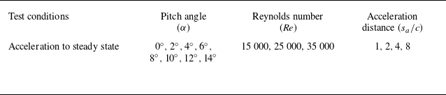
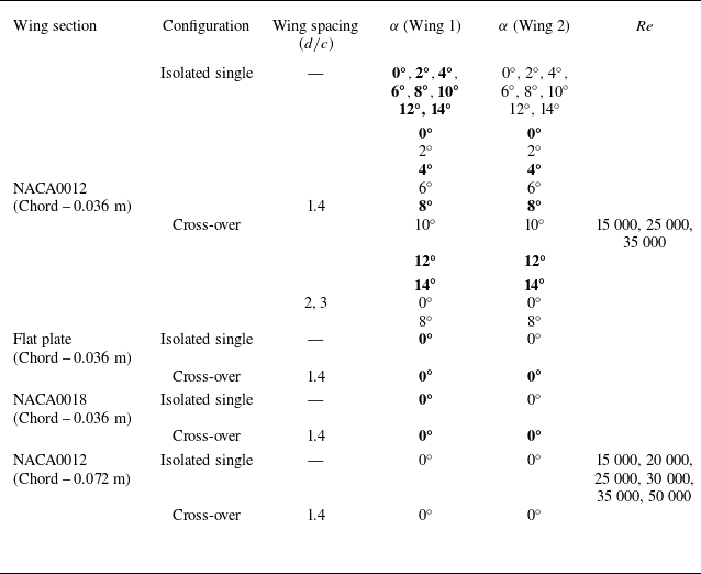

 cl
 α=6∘
 Re=25000
 sa/c=2

 cl
 cd
 cm
 cl
 W1
 W2
 T1
 T2
 cd
 cm
 Re=25000
 35000
 Re=40000

 α=0∘
 α=4∘
 s/c
 s/c=0
 1.4c
 α=0∘
 α=4∘

 α=0∘
 α=0∘
 α=4∘
 α=4∘
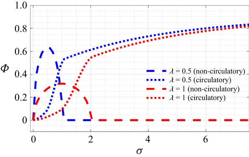
 λ=0.5
 λ=1

 λ=0.5
 λ=1
 α=0∘
 α=4∘
 α=0∘
 α=4∘

 α=0∘

 (δcl)max
 (s/c)(δcl)max
 Re=15000
 Re=25000
 Re=35000

 δcl
 Re=15000,25000,35000
 (δcl)max
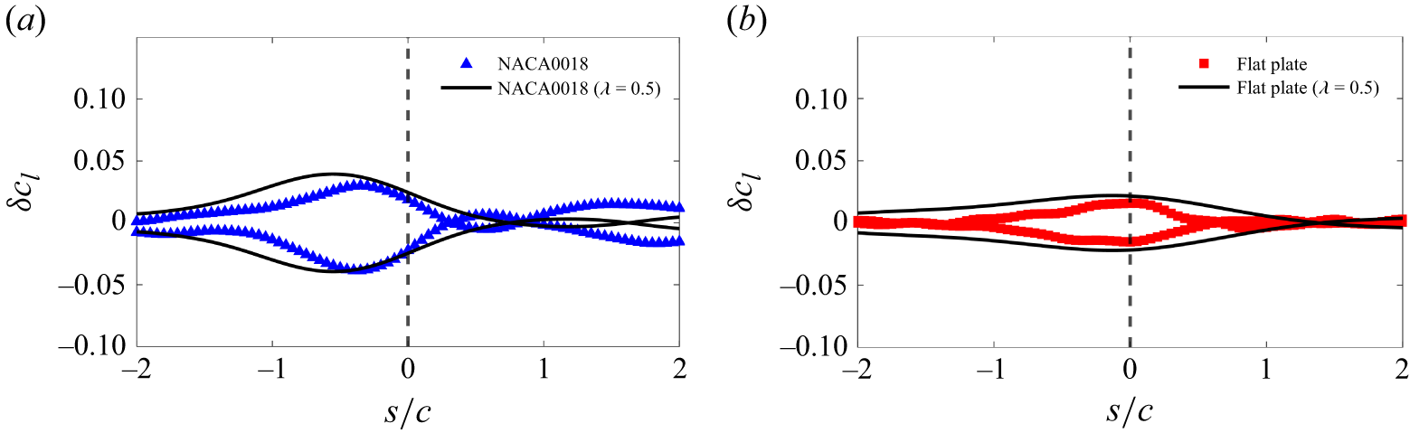
 λ=0.5
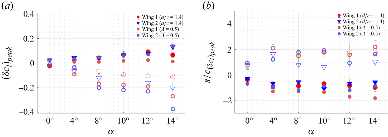
 cl

 α=8∘,10∘,12∘
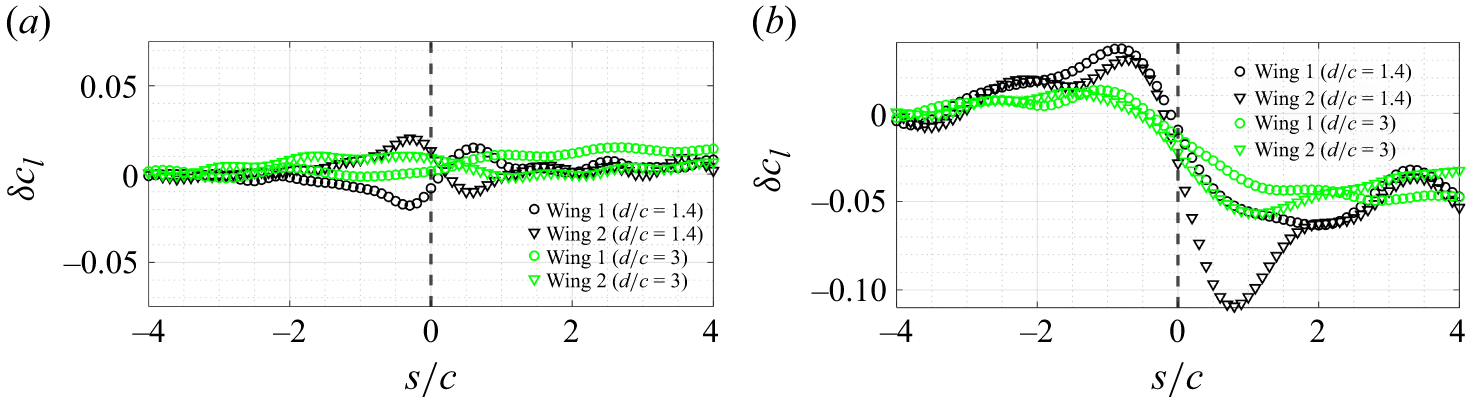
 α=0∘
 α=8∘


 Open access

