


1. Introduction
Turbulence is arguably one of the most difficult subjects in nonlinear physics due to its complex and challenging mathematical descriptions, its inherent instabilities and chaotic nature (Sun Reference Sun2019). The presence of a wall compounds further the challenge to investigate turbulence, such as in turbulent boundary layers. In addition, complications arise when the wall is rough.
Rough wall flows tend to produce a higher coefficient of friction  $(C_{f}=2\tau _{w}/\rho U_{\infty }^{2}$, where
 $U_{\infty }$ is the free-stream velocity,
 $\tau _{w}$ is the wall shear stress and
 $\rho$ is the density of the fluid), than flows over smooth surfaces. The increase of
 $C_{f}$ is manifested in the downward shift of the wall–unit normalised mean velocity profile when compared with the smooth wall profile (Hama Reference Hama1954). The shift, known as the roughness function, is defined as
 $\Delta U^{+}=\Delta U/U_{\tau }$, where
 $U$ is the mean streamwise velocity and
 $U_{\tau }$ is the friction velocity
 $U_{\tau }=\sqrt {\tau _{w}/\rho }$; the superscript, (
 $^{+}$) means normalisation by the wall units
 $U_{\tau }$ or
 $\nu /U_{\tau }$, where
 $\nu$ is the kinematic viscosity. The roughness function is a function of the equivalent sand grain roughness
 $k_{s}$ (Schlichting & Kestin Reference Schlichting and Kestin1961). Ideally, one would like to determine
 $\Delta U^{+}$ based solely on the roughness topology. This would provide a way of predicting
 $C_{f}$ without the need to perform lengthy measurements. Unfortunately,
 $k_{s}$ is not a physical roughness parameter and its determination relies on an empirical method based on the mean velocity profile (Nikuradse Reference Nikuradse1933).
When  $k_{s}^{+}$ is large enough the flow is considered to be in the ‘fully rough’ regime and the drag is mainly composed of the pressure (or form) drag (Squire et al. Reference Squire, Morrill-Winter, Hutchins, Schultz, Klewicki and Marusic2016). This regime is characterised by a log–linear relationship between
 $\Delta U^{+}$ and
 $k_{s}^{+}$. On the other hand, when
 $k_{s}^{+}$ is too small, the roughness does not have a noticeable effect on the viscous sublayer of the flow. This flow regime is called ‘dynamically smooth’ and can be treated as a smooth wall flow. At moderate values of
 $k_{s}^{+}$, both the pressure drag and the viscous drag contribute to the total drag. This flow regime is called ‘transitionally rough’ (Nikuradse Reference Nikuradse1933). So far there are no clear thresholds that delimit these flow regimes. However, it is commonly agreed that the flow is hydraulically smooth when
 $k_{s}^{+} < 4$, and fully rough when
 $k_{s}^{+} > 70$ (Jiménez Reference Jiménez2004).
The roughness function  $\Delta U^{+}$ is determined by ‘measuring’ the vertical shift between the log regions of the rough wall and smooth wall wall-unit normalised velocity profiles. This requires that experiments be conducted for each rough surface to obtain the velocity profile and friction velocity. A more practical way to proceed, but one that also presents a big challenge, is to predict
 $\Delta U^{+}$ directly from surface topology or by other means, correlating
 $k_{s}$ to one or more parameters characterising the roughness. So far, there has been no definite consensus on which length scale or roughness parameter best characterises a surface that can correlate with the friction drag. Over the last decade, a large body of work has been undertaken to address this issue (Musker Reference Musker1980; Napoli, Armenio & De Marchis Reference Napoli, Armenio and De Marchis2008; Schultz & Flack Reference Schultz and Flack2009; Forooghi et al. Reference Forooghi, Stroh, Magagnato, Jakirlić and Frohnapfel2017; Flack, Schultz & Barros Reference Flack, Schultz and Barros2020, among many others). A wide range of different surface parameters has been studied to predict which of these parameters dominantly affects the friction drag. Some of these parameters are the mean roughness height
 $k_{a}$, root-mean-square height
 $k_{rms}$, maximum peak to valley height
 $k$, average peak to valley height
 $k_{z}$, effective slope
 $ES$, solidarity
 $\lambda _{f}$, skewness
 $k_{sk}$ and flatness
 $k_{ku}$. However, none of these parameters is sufficient to be generalised for all kinds of roughness.
Musker (Reference Musker1980) developed a modified roughness Reynolds number as a function of simple geometric statistics (average absolute slope, standard deviation, skewness and flatness) for naturally occurring surfaces as follows:
 \begin{equation} k_{s}^{+} = \frac{\sigma U_{\tau}}{\nu}(1+aES)(1+bk_{sk}k_{ku}),\end{equation}
where  $a$ and
 $b$ are constants to give the best fit of roughness functions related to naturally occurring surfaces, and
 $\sigma$ is the standard deviation of the surface roughness.
Waigh & Kind (Reference Waigh and Kind1998) studied a regular three-dimensional (3-D) roughness and found that the element bluntness and spanwise aspect ratio are the main parameters characterising the roughness function as follows:
 \begin{align} \Delta U^{+} = \left\{
\begin{array}{@{}ll}
10.56\log\left[\left(\dfrac{1}{\lambda_{f}}\dfrac{k}{b_{m}}\right)^{0.87}
\left(\dfrac{A_{w}}{A_{f}}\right)^{0.44}\right] - 7.59 &
\varLambda <6,\\
-5.57\log\left[\left(\dfrac{1}{\lambda_{f}}\dfrac{k}{b_{m}}\right)^{0.55}
\left(\dfrac{A_{w}}{A_{f}}\right)^{1.38}\right] + 5.78 &
\varLambda > 6, \end{array}
\right.\end{align}
where  $\varLambda = \lambda _{f} k/s_{m}$,
 $s_{m}$ is the streamwise width of the roughness element,
 $b_{m}$ is the spanwise width of the roughness element,
 $\lambda _{f}=A_{f}/A_{s}$,
 $A_{s}$ is the surface area,
 $A_{f}$ is the projected frontal area and
 $A_{w}$ is the wetted area.
Bons (Reference Bons2002) derived a new  $k_{s}$ correlation, based on the surface slope angle for real turbine roughness; the roughness panels were scaled models of actual turbine surfaces instead of using the traditional simulated roughness
 \begin{equation} k_{s} ={-}0.0261 ES + 0.0138 ES^{2}.\end{equation}
Schultz & Flack (Reference Schultz and Flack2009) studied close-packed pyramid roughnesses to study the effect of the height and slope of roughness on the flow. They found that  $\Delta U^{+}$ mainly depends on the roughness height. They also found a range of
 $ES$ such that, below this level, the surface is considered to be wavy, not rough, and the roughness function strongly depends on the
 $ES$. If
 $ES < 0.35$, the surface is considered to be wavy.
Forooghi et al. (Reference Forooghi, Stroh, Magagnato, Jakirlić and Frohnapfel2017) investigated numerically the effect of various roughness parameters on  $k_{s}$ in the fully rough regime of channel flow at friction Reynolds number
 $Re_{\tau }\approx 500$. Their roughness geometries were generated by systematically changing the moments of the surface height probability density function, the effective slope of the random roughness and the size distribution of the roughness peaks. Forooghi et al. (Reference Forooghi, Stroh, Magagnato, Jakirlić and Frohnapfel2017) correlate
 $k_{s}$ based on
 $k$,
 $k_{sk}$ and
 $Es$. They found that these roughness parameters can predict
 $k_{s}$ accurately for randomly distributed roughness in the fully rough regime of channel flows
 \begin{gather} \left. \begin{gathered}
{k_{s}/k = F(k_{sk})G(ES)},\\ {F(k_{sk}) =
0.67k_{sk}^2+0.93k_{sk}+1.3},\\ {G(ES) = 1.07(1-{\rm
e}^{{-}3.5ES})}.
\end{gathered}\right\}\end{gather}
Flack et al. (Reference Flack, Schultz and Barros2020) investigated the importance of roughness height and skewness on the coefficient of friction. A  $k_{s}$ correlation was derived as
 \begin{equation} k_{s} = A_{1} k_{rms}(1+k_{sk})^{B_{1}},\end{equation}
with  $A_{1}=4.43$ and
 $B_{1}=1.37$.
While many roughness function formulations in terms of one or more roughness parameters have been proposed recently, they are limited to the particular roughness investigated. In other words, they lack universality. This is certainly associated with the fact that, so far, a ‘universal’ critical parameter for all roughnesses is yet to be determined. Whether such ‘universal’ parameter exists or not is still an open issue. It is nevertheless conceivable that such parameter can be identified for families of rough surfaces, such as 2-D roughness and 3-D roughness, in the fully rough regime. The present work is an attempt to determine such a parameter with the view to develop an expression for  $k_{s}$. The roughness family considered here is that of 2-D roughness. One reason to focus on this roughness family is that it was shown to produce a fully rough regime at relatively low Reynolds number, which can be easily achieved in wind tunnels. For example the use of 2-D rods attached to a smooth wall where the spacing between two consecutive rods,
 $s_{x}$, is approximately 8
 $k$ leads to a fully rough regime (Djenidi, Talluru & Antonia Reference Djenidi, Talluru and Antonia2018). In their direct numerical simulations of a turbulent rough wall channel flow, Leonardi et al. (Reference Leonardi, Orlandi, Smalley, Djenidi and Antonia2003) used transverse square bars as a roughness, with
 $s_{x}$ varying from 2
 $k$ to 32
 $k$. They showed that the form drag was the main contributor to the total drag when 8
 $k \leq s_{x} \leq$ 16
 $k$. Later, Leonardi et al. (Reference Leonardi, Orlandi, Djenidi and Antonia2015) used circular rods and investigated friction and pressure drags numerically, confirming their previous observations. Kamruzzaman et al. (Reference Kamruzzaman, Djenidi, Antonia and Talluru2015) investigated the turbulent boundary layer developed over a rod roughened wall that has a spacing between two consecutive rods of 8
 $k$. They calculated the pressure drag directly from the distribution of static pressure around one rod. They revealed that
 $C_{f}$ is constant and independent of the Reynolds number in the fully rough regime. This was further confirmed by Djenidi et al. (Reference Djenidi, Talluru and Antonia2018).
In this present work, we carry out turbulent boundary layer measurements over various 2-D rough surfaces with a height ratio  $\delta /k$ ranging from 23 to 41. Two sets of experiments are conducted. The first one is to validate our rough wall measurements and estimation of
 $U_{\tau }$. Also, the experiments are used to validate the Reynolds number independence when the flow is fully rough. The second set of experiments is exploited to determine the most critical dominant roughness parameters impacting
 $C_{f}$ with the view to developing an expression for
 $k_{s}^{+}$ valid for the 2-D rough wall family.
2. Experimental details
2.1. Wind tunnel facility
The experiments are performed in a closed-return-type wind tunnel located at the University of Adelaide. It can achieve a maximum velocity of 30 m s $^{-1}$ with a low-level turbulence intensity of approximately 0.53 %. The test section is rectangular and has a cross-section of
 $500\ {\rm mm} \times 300\ {\rm mm}$ and a 2000 mm length. A 125 mm long circulation flap is also installed downstream of the test section to reduce the circulations generated over the flat plates as much as possible and to make sure that the stagnation point is on the measurement side of the plate. This flap can be regulated to keep the flow with a zero pressure gradient (ZPG) along with adjusted sidewalls. The tunnel should be wider than six times the boundary layer thickness to ensure the boundary layer developed in the test section is two-dimensional, as reported by Nickels et al. (Reference Nickels, Marusic, Hafez and Chong2005). In our measurements, the 500 mm width is more than
 $7 \delta$ of the largest boundary layer thickness developed. The inlet flow is tripped by a
 $4$ mm diameter rod and a
 $100$ mm strip of sandpaper with a
 $40$ grit number.
2.2. Surface roughness
The roughness details of this study are: circular rods of 500 mm length with two different diameters,  $k = 1.6$ and 2.4 mm, and five different streamwise spacing ratios
 $s_{x}/k$ ranges from 6 to 24. A total of 30 plates, 3-D printed triangular ribs, of
 $k = 1.6$ mm and
 $8k$ spacing; each plate measures
 $145\ {\rm mm} \times 153.6\ {\rm mm}$. The 3D printed triangular ribs were printed from acrylonitrile butadiene styrene (ABS) plastic material using a fused deposition modelling 3D printer, Zortrax M200. This model has an accuracy of 200
 $\mathrm {\mu }$m in the
 $x$ and
 $z$ directions, and a layer height of 90
 $\mathrm {\mu }$m with a
 $0.4$ mm nozzle diameter, where
 $x$ and
 $z$ are the streamwise and spanwise directions, respectively. A total of 8 CNC machined plates are employed, each of which has a 2-D sinewave surface function, an amplitude of
 $k/2 = 0.8$ mm and a wavelength of
 $8k$; each plate measures
 $435\ {\rm mm} \times 192\ {\rm mm}$. These CNC machined surfaces were machined by a custom carbide engraving cutter of a TORMACH PCNC-series 3 machine. Two CNC machined plates have a 2-D sinewave surface function, an amplitude of
 $k/2 = 1.2$ mm and a wavelength of
 $8k$; each plate measures
 $480\ {\rm mm} \times 768\ {\rm mm}$. This surface was fabricated by a Multicam M1212 Router machine, with a 0.6 mm stepover and 12 mm ball nose cutter. The absolute values of the profile heights for different rough surfaces are described as follows: a periodic function describes the rough surface of the circular rods, triangular ribs and sinewaves, respectively, as follows:
 $$\begin{gather} Z(x) = \left\{\begin{array}{@{}ll} \sqrt{kx-x^{2}} & 0 \leq x \leq k,\\ \dfrac{-k}{2} & k< x< s_{x}, \end{array} \right. \end{gather}$$
 $$\begin{gather}Z(x) = \left\{ \begin{array}{@{}ll} \dfrac{-k}{2}+\dfrac{2kx}{s_{x}} & 0 \leq x \leq s_{x}/2,\\ \dfrac{-k}{2}+\dfrac{2k(s_{x}-x)}{s_{x}} & s_{x}/2 \leq x \leq s_{x}, \end{array} \right. \end{gather}$$
 $$\begin{gather}Z(x) = \frac{k}{2}\sin\left(\frac{2{\rm \pi} x}{s_{x}}\right), \end{gather}$$
where  $k=1.6$ mm and
 $s_{x}=8k$. The surfaces are defined by the first letter of the shape name:
 $R$ for rods,
 $T$ for triangular ribs and
 $S$ for sinewaves followed by
 $10k$ and finally the spacing ratio between two consecutive roughness peaks. For example
 $R16-08$ means a surface with cylindrical rods with a height of 1.6 mm and spacing ratio between two consecutive roughness rods of
 $8$. All different roughnesses, as well as the strip of sandpaper are taped using double-sided tape on an aluminium sheet of dimensions
 $500 {\rm mm} \times 1600\ {\rm mm}$. Statistical parameters used to characterise the different rough surfaces are tabulated in table 1.
Different key surface roughness parameters.

The roughness average height  $k_{a}$, is defined by ASME (2009) as the arithmetic average of the absolute values of the profile height deviations from the mean
 $m$ line, defined on the sampling length
 $L_{s}$ as
 \begin{equation} k_{a} = \frac{1}{L_{s}}\int_{0}^{L_{s}}|Z(x)-m|\,{{\rm d}\kern0.7pt x}.\end{equation}
The root-mean-square height  $k_{rms}$ corresponds to the standard deviation
 $\sigma$ of the height distribution, defined on the sampling length as
 \begin{equation} k_{rms} = \sqrt{\frac{1}{L_{s}}\int_{0}^{L_{s}}Z(x)^{2}\,{{\rm d}\kern0.7pt x}}.\end{equation}
The roughness skewness  $k_{sk}$ (normalised third-order moment), is the asymmetry of the height distribution, defined on the sampling length. This parameter is crucial, as it indicates a morphology of the surface texture (see Flack et al. Reference Flack, Schultz, Barros and Kim2016). Positive values correspond to high peaks spread on a regular surface, while negative values correspond to surfaces with pores and scratches. However, this parameter does not give any information about the absolute height of the profile, contrary to
 $k_{a}$
 \begin{equation} k_{sk} = \frac{1}{\sigma^3L_{s}}\int_{0}^{L_{s}}(Z(x)-m)^{3}\,{{\rm d}\kern0.7pt x}.\end{equation}
The roughness kurtosis  $k_{ku}$ (normalised fourth-order moment), is the sharpness of the height distribution, defined on the sampling length as
 \begin{equation} k_{ku} = \frac{1}{\sigma^4L_{s}}\int_{0}^{L_{s}}(Z(x)-m)^{4}\,{{\rm d}\kern0.7pt x}.\end{equation}
The equation for the effective slope  $ES$, which is the mean absolute streamwise gradient of the surface, as defined by Napoli et al. (Reference Napoli, Armenio and De Marchis2008) for 2-D rough surfaces is as follows:
 \begin{equation} ES = \frac{1}{L_{s}}\int_{0}^{L_{s}}\left|\frac{{\rm d}Z(x)}{{\rm d}\kern0.7pt x}\right|\,{{\rm d}\kern0.7pt x}, \end{equation}
this parameter is also related to the solidity  $\lambda _{f}$, which is defined as the total projected frontal area of the roughness element
 $A_{f}$ per unit wall parallel area
 $A_{p}$, by the relationship
 $ES=2\lambda _{f}$ (see Napoli et al. Reference Napoli, Armenio and De Marchis2008)
 \begin{equation} \lambda_{f} = \frac{A_{f}}{A_{p}}.\end{equation}
2.3. Measurement rig
Single hot-wire probes with 5  $\mathrm {\mu }$m diameter tungsten wire, and 1 mm sensing length
 $(l)$ are used in measurements to give a length to diameter ratio of approximately
 $200$, as recommended by Ligrani & Bradshaw (Reference Ligrani and Bradshaw1987) and Hutchins et al. (Reference Hutchins, Nickels, Marusic and Chong2009). An overheat ratio of
 $1.6$ is applied using an IFA300 constant temperature anemometer. A T-type thermocouple integrated with the IFA300 is used to record the mean temperature in the free stream throughout the experiment. Dynamic calibration of the hot-wire is performed with a square wave test also integrated into the IFA300 to determine the cutoff frequency of the hot-wire. A
 $-$3 dB drop off at approximately 10 kHz is recorded. Static calibration of the hot-wire is performed before and after each experiment. Calibrations are performed in situ against the Pitot-static tube positioned in the free-stream flow. More than 20 different velocities ranging between zero and 1.2 of the free-stream velocity of the experiment, are used for the calibration. If the pre-and post-calibrations do not collapse well, with a maximum 2 % error, the measurement is repeated. A polynomial of order six is used for fitting the voltage of the hot-wire and the measured velocity from the Pitot-static tube. Linear interpolation between pre-and post-calibrations are used to account for the hot-wire voltage drifting during the whole experiment.
A high magnification digital microscope is used to determine the offset from the wall at the first measurement point. The microscope is mounted on a 3D printed plate and placed on the rough surfaces to determine the wall offset. The probe is moved down to a distance of 100  $\mathrm {\mu }$m over the plate before removing the plate. Then, the probe is moved down by a specific distance. This distance is equal to the thickness of the plate, plus the 100
 $\mathrm {\mu }$m offset, plus half of the roughness height
 $( 20 + 0.1 + k/2)$ mm. Thus
 $y = 0$ is located at the midpoint of the roughness element height. The criterion for choosing this location is detailed in § 3. Measurements are taken at the midpoint of two consecutive roughness peaks at
 $x \approx 1.5$ m downstream, measured after the tripping sandpaper. A total of
 $48$ logarithmically spaced measurement points along the wall-normal position are taken by a Mitutoyo height gauge with a linear glass encoder attached to it, with 1
 $\mathrm {\mu }$m resolution, to determine the distance travelled away from the wall accurately. Measurements are taken with a sampling rate of
 $35$ kHz for each wall-normal location. Figure 1 shows a schematic of the different rough surface set-ups and the measurement location.
Schematic of different surface geometry set-ups with the same  $k=1.6$ mm and
 $s_{x}=8k$. The red dotted line shows the measurement location. The coordinate system used in the experiments and
 $y=0$ as a reference point are indicated in the schematic.

2.4. Experiments
Two sets of experiments are conducted. In the first set the free-stream velocity  $U_{\infty }$ is varied from
 $5$ to
 $20$ m s
 $^{-1}$ over 2-D circular rods of
 $k=1.6$ mm diameter and
 $8k$ spacing. The results are validated with data from Djenidi et al. (Reference Djenidi, Talluru and Antonia2018) with almost the same roughness, and the same
 $Re_{\tau }$ range from
 $1300$ to
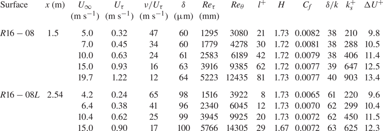
 $5220$. The boundary layer thicknesses are different because of the variation of the measurement location. The details of the first set of experiments are indicated in table 2. The first set aims to validate our measurements and calculation of the friction velocity
 $U_{\tau }$, as well as validate the fully rough Reynolds number independence and the consistency of the coefficient of friction
 $C_{f}$ in the fully rough regime.
Details of the first set of rough wall experimental data.  $R16-08L$ refer to Djenidi et al. (Reference Djenidi, Talluru and Antonia2018) data.

For the second set of experiments, measurements over different rough surfaces such as rods, triangular ribs and sinewaves, are carried out. All measurements in the second set are in the fully rough regime where  $k_{s}^{+}>100$, with three different free-stream velocities ranging from
 $10$ to
 $23$ m s
 $^{-1}$ for each surface. The boundary layer thickness varied from
 $48$ to
 $70$ mm (
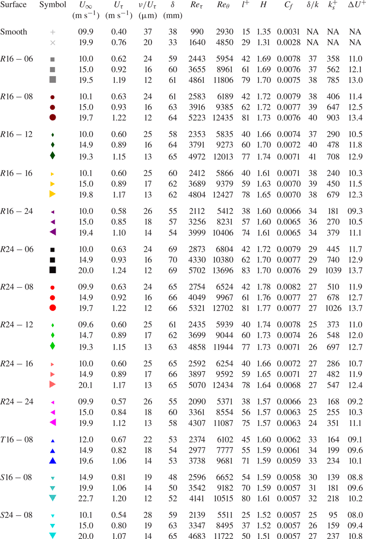
 $23 < \delta /k < 41$). All information and details of the second set of data are presented in table 3. This set is used to investigate dominant roughness parameters that affect the turbulence statistics as well as the drag coefficient and correlate them directly to the roughness function.
Details of the second set of rough wall experimental data.

3. Friction velocity
One of the challenges of turbulent boundary layer (TBL) measurements over a rough surface is the calculation of the friction velocity  $U_{\tau }$. Clauser (Reference Clauser1956) introduced a method, the Clauser chart method, widely used for smooth wall TBL. The method consists of fitting measured velocity profile data to the so-called law of the wall
 \begin{equation} U^{+} = \frac{1}{\kappa}\ln y^{+}+B,\end{equation}
where  $\kappa$ is the von Kármán constant and
 $B$ is an additive constant. Unfortunately, the method has some uncertainties, such as the values of
 $\kappa$,
 $B$ and the lower and upper limits of the overlap region. For rough surface TBLs, the method requires two more variables, adding further uncertainties (Perry & Joubert Reference Perry and Joubert1963) since the law of the wall becomes
 \begin{equation} U^{+} = \frac{1}{\kappa}\ln \frac{(y+\epsilon) U_{\tau}}{\nu}+B-\Delta U^{+},\end{equation}
where  $\epsilon$ is an origin offset.
Marusic et al. (Reference Marusic, Monty, Hultmark and Smits2013) carried out measurements on high Reynolds number smooth wall TBLs. They found that the boundaries of the log region that best fit the velocity profiles are  $y^{+} > 3\sqrt {Re_{\tau }}$ and
 $y/\delta = 0.15$, which will be adapted in the present study as they best fit the log region of the velocity profiles over rough surfaces as well. Recently, Djenidi, Talluru & Antonia (Reference Djenidi, Talluru and Antonia2019) proposed a method for estimating
 $U_{\tau }$ for both smooth and rough wall TBLs. The method assumes an outer layer similarity between the smooth and rough flow and uses the velocity defect distribution, which is shown to exhibit a universal form for these two TBLs. A practical advantage of this latter method is that it involves empirical constants, thus eliminating the uncertainties of the modified Clauser chart method.
In the present work both the modified Clauser chart (Perry & Li Reference Perry and Li1990) and the velocity defect chart (Djenidi et al. Reference Djenidi, Talluru and Antonia2019) methods will be used. Regarding the modified Clauser chart method, we performed a detailed study of the effect of  $\kappa$ and
 $\epsilon$ on the estimate of
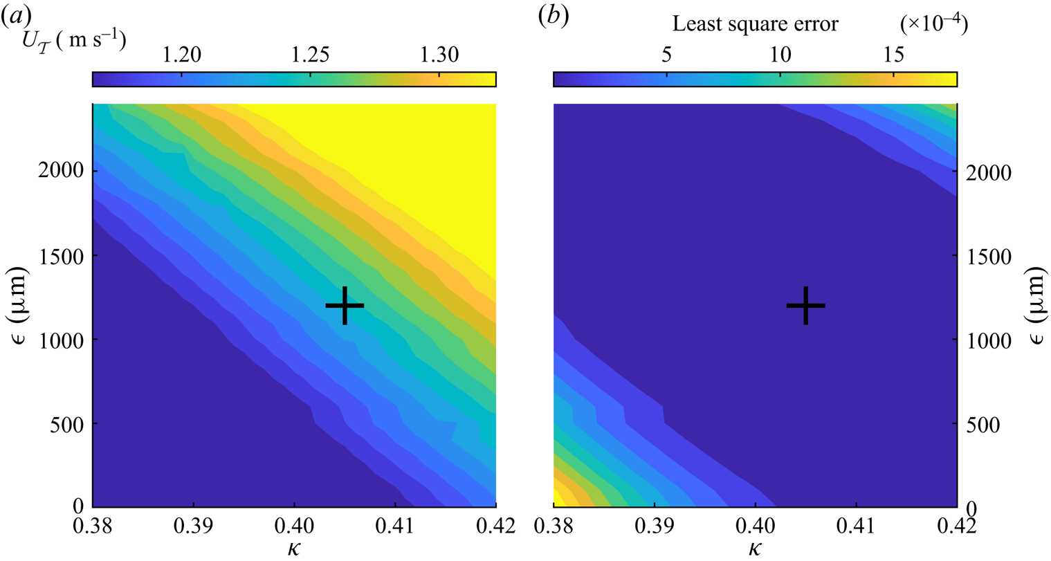
 $U_{\tau }$, in an attempt to understand how these parameters affect the results. Estimates based on both methods are compared. Figure 2(a) shows the values
 $U_{\tau }$, based on the modified Clauser chart, for different values of
 $\epsilon$ and
 $\kappa$ over the
 $R24-06$ surface at
 $U_{\infty } = 20$ m s
 $^{-1}$;
 $\epsilon$ varies from 0 to
 $k$ while
 $\kappa$ ranges from 0.38 to 0.42. The least squares error of the fitting equation in the log region is shown in figure 2(b). Results for different free-stream velocities and different surface roughnesses follow the same pattern of contours and are not shown here. These contours also show an infinite number of solutions that can be fitted with the same least squares error, illustrating the strong reliance on
 $\epsilon$ and
 $\kappa$ of the modified Clauser chart method, and thus somehow its weakness. Figure 2(a) indicates that the maximum deviation for
 $U_{\tau }$ when using the modified Clauser chart is approximately 10 %. Figure 2(b) shows that
 $\kappa \approx 0.4$ gives the smallest error, regardless of the value of
 $\epsilon$. Also, using
 $k/2 < \epsilon < 3k/4$ yields the same minimum error from fitting the mean velocity profile by the modified Clauser method regardless of the value of
 $\kappa$. The roughness function
 $\Delta U^{+}$ is determined by averaging the vertical shift between the log region (
 $y^{+} > 3\sqrt {Re_{\tau }}$ to
 $y/\delta = 0.15$) of the rough wall and smooth wall wall-unit normalised velocity profiles.
Friction velocity and least square error of TBL measurement over the  $R24-06$ surface at
 $Re_{\tau } = 5700$. (a) Contours of
 $U_{\tau }$ calculated from the modified Clauser chart. (b) Contours of least squares error from fitting data to the modified Clauser chart. The plus mark
 $(+)$ refers to
 $\kappa = 0.405$ and
 $\epsilon =k/2= 1200\ \mathrm {\mu }$m.

Since the main goal of the present study is to compare various roughness geometries and the focus of the results is on the outer layer similarity, we fix  $\epsilon = k/2$ for all rough walls under investigation with
 $\kappa \approx 0.405$ and
 $B = 5$. Fixing these values, we found that
 $U_{\tau }$ obtained from the modified Clauser chart method matches that obtained from the velocity defect chart with an error of less than 3 % for all Reynolds numbers considered. The value of
 $U_{\tau }$ obtained from the velocity defect chart is used in the presented results for all rough wall flows, since the values obtained from both methods show good agreement.
4. Results
4.1. Validation
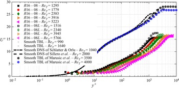
Streamwise mean velocity profiles of the TBL over the  $R16-08$ surface, normalised by inner scaling parameters at different
 $Re_{\tau }$, are plotted with filled symbols in figure 3. For comparison with our measurements, the data of Djenidi et al. (Reference Djenidi, Talluru and Antonia2018) at comparable
 $Re_{\tau }$ are represented with unfilled symbols. Also, our smooth wall data measurements are compared with the smooth TBL direct numerical simulation (DNS) data of Schlatter & Örlü (Reference Schlatter and Örlü2010) and Sillero, Jiménez & Moser (Reference Sillero, Jiménez and Moser2014) for
 $Re_{\tau }=1040$ and
 $Re_{\tau }=2000$, respectively. Two sets of smooth wall TBL experimental data (Marusic et al. Reference Marusic, Chauhan, Kulandaivelu and Hutchins2015) are also reported on the figure for comparison. As expected, all smooth wall data collapse very well in the buffer and log regions. The friction velocity for smooth wall measurements is calculated by the Clauser method with
 $\kappa =0.405$ and
 $B=5$.
The streamwise mean velocity profiles over the  $R16-08$ surface at different free-stream velocities normalised by the friction velocity
 $U_{\tau }$. The unfilled symbols represent data from Djenidi et al. (Reference Djenidi, Talluru and Antonia2018) at the closest
 $Re_{\tau }$. Our smooth wall TBL measurements are plotted in grey symbols and are detailed in table 3. The dot-dashed line shows the smooth DNS data from Schlatter & Örlü (Reference Schlatter and Örlü2010) at
 $Re_{\tau }=1040$. The dashed line shows the smooth DNS data from Sillero et al. (Reference Sillero, Jiménez and Moser2014) at
 $Re_{\tau }=2000$. The black and blue hexagram symbols are smooth TBL data from Marusic et al. (Reference Marusic, Chauhan, Kulandaivelu and Hutchins2015) at
 $Re_{\tau }= 3500$ and 4000, respectively. The wall-normal position
 $y$ is normalised by the inner length scale
 $\nu /U_{\tau }$.

Using 2-D cylindrical rods for roughening a surface leads to a fully rough regime at a relatively low  $Re_{\tau }$. All rough data in figure 3 are in a fully rough regime, as indicated in table 2. Increasing
 $Re_{\tau }$, or equivalently
 $U_{\infty }$, once the fully rough regime is achieved causes a rightwards shift towards larger
 $y^{+}$, while
 $U^{+}=U/U_{\tau }$ (or
 $C_{f}\sim \sqrt {U_{\tau }/U}$) remains constant. The present data are in good agreement with the data of Djenidi et al. (Reference Djenidi, Talluru and Antonia2018), especially at
 $Re_{\tau }$ higher than 4000. The rightwards shift towards larger
 $y^{+}$ while maintaining the same
 $C_{f}$ suggests that the inner length scale
 $\nu /U_{\tau }$ is not an adequate scaling length for rough wall mean streamwise velocity profiles.
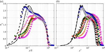
Profiles of streamwise root-mean-square (r.m.s.) velocity fluctuating  $u^{\prime +}$ for the
 $R16-08$ surface are reported in figures 4(a) and 4(b) as functions of
 $y/\delta$ and
 $y/U_{\tau }/\nu$, respectively. Figure 4(a) shows an excellent collapse in the outer layer
 $y/\delta >0.6$, regardless of the Reynolds number or the roughness of the surface. The present rough and smooth wall data exhibit lower magnitudes than those of Djenidi et al. (Reference Djenidi, Talluru and Antonia2018) and Marusic et al. (Reference Marusic, Chauhan, Kulandaivelu and Hutchins2015) in the near-wall region. This is believed to be due to larger values of our
 $l^{+}$, which may attenuate the actual values of
 $u^{\prime +}$. Nevertheless, this has a negligible effect on the scope of the work as our focus is on comparing different kinds of roughnesses in terms of their effects on the mean velocity profiles. Chin et al. (Reference Chin, Hutchins, Ooi and Marusic2009) investigated spatial resolution issues in hot-wire measurements of wall-bounded turbulent flows. They applied different spanwise filter lengths to channel flow DNS data streamwise velocity components to simulate different spatial resolutions of single hot-wire probes. They found that the most severe attenuation occurs in the near-wall region due to the dominance of the small turbulence scales in this region. These attenuations are less severe in the outer region and are practically negligible for
 $y/\delta >0.6$.
Profiles of  $u^{\prime }$ over the
 $R16-08$ surface at different free-stream velocities normalised by the friction velocity
 $U_{\tau }$. The symbols are the same as indicated in figure 3. (a) The wall-normal position
 $y$ is normalised by the outer length scale
 $\delta$. (b) The wall-normal position
 $y$ is normalised by the inner length scale
 $\nu /U_{\tau }$.

Figure 4(b) shows a noticeable systematic shift of the  $u^{\prime +}$ profiles when plotted as a function of
 $y^{+}$. The rightward shift is similar to that observed in
 $U^{+}$ as
 $Re_{\tau }$ increases, further confirming that the inner length scale
 $\nu /U_{\tau }$ is not an appropriate scaling length. For the rough wall data, one can observe a local inner peak at low Reynolds which tends to vanish as the Reynolds number increases. This behaviour is consistent with that observed in Schultz & Flack (Reference Schultz and Flack2007), Krogstad & Efros (Reference Krogstad and Efros2012), Squire et al. (Reference Squire, Morrill-Winter, Hutchins, Schultz, Klewicki and Marusic2016) and Djenidi et al. (Reference Djenidi, Talluru and Antonia2018), further indicating that the possible attenuation associated with the relatively large values of
 $l^{+}$ does not critically affect the data, at least qualitatively in the inner region, giving us confidence in our measurements.
4.2. Second set of experiments
4.2.1. Mean velocity profile
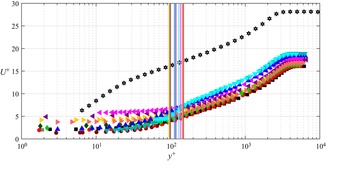
Figure 5 shows the distributions  $U^{+}$ vs
 $y^{+}$ for all the different rough surfaces used in this study; the vertical lines correspond to
 $y=k$ and their colours match those of the profiles they are associated with. For each rough wall, only one velocity distribution corresponding to a fully rough regime is reported;
 $Re_{\tau }$ ranges from 3300 to 4300. Also, the smooth wall velocity distribution data of Marusic et al. (Reference Marusic, Chauhan, Kulandaivelu and Hutchins2015) at
 $Re_{\tau }=3500$ are shown in the figure as reference.
Streamwise mean velocity profiles over different rough surfaces at matched Reynolds number  $3300< Re_{\tau }<4300$ where each surface is normalised by the friction velocity
 $U_{\tau }$. The symbols of our measurements are detailed in table 3. The black hexagram symbols are smooth TBL data from Marusic et al. (Reference Marusic, Chauhan, Kulandaivelu and Hutchins2015) at
 $Re_{\tau }=3500$. The wall-normal position
 $y$ is normalised by the inner length scale
 $\nu /U_{\tau }$. The vertical lines indicate the roughness heights in terms of viscous length scale units
 $k^{+}$.

As we mentioned earlier, in a fully rough regime and at high Reynolds numbers, increasing the Reynolds number simply shifts the mean velocity profile to the right, to larger  $y^{+}$, while
 $C_{f}$ remains constant. Roughnesses with the same spacing ratio
 $s_{x}/k$ are represented by the same symbol, while the colours indicate different roughness heights, as indicated in table 3. If we consider the rod and sinewave roughnesses and consult table 1, we note that keeping
 $s_{x}$ constant while changing
 $k$ does not change
 $k_{sk}$,
 $k_{ku}$,
 $ES$ and
 $\lambda _{f}$. Thus, the excellent collapse we observe between the distribution
 $s_{x}$ for the rod and sinewave rough wall suggests that, in the fully rough regime, changing
 $k$ or
 $\delta /k$ does not affect the mean streamwise velocity profile if
 $\delta /k$ is large enough (
 $\delta /k>23$ in the present case). Changing of the spacing ratio between rods from 6 to 24 while maintaining the same roughness height causes a downward shift as a result of an increase of
 $C_{f}$. Decreasing the
 $s_{x}/k$ ratio, which results in an increase of the effective slope
 $ES$ and a decrease of the skewness
 $k_{sk}$ for the same geometry, leads to a larger
 $C_{f}$ with a resulting downward shift. More details about the effect of roughness parameters on the coefficient of friction will be discussed later, in § 4.2.4.
The velocity profiles for the rods with spacing ratios of  $6$ and
 $8$ collapse relatively well, indicating that the boundary layer is only marginally affected by the small change of
 $s_{x}$, which is illustrated by the fact that
 $C_{f}$ values for both spacing ratios are practically the same (see table 3). This is consistent with DNS data of Leonardi et al. (Reference Leonardi, Orlandi, Smalley, Djenidi and Antonia2003) which show that the drag in a rod roughened turbulent channel flow is practically unchanged for
 $6 \leq s_{x}/k \leq 8$. Similar results are also observed in the data for a TBL over a rod roughened wall in Furuya, Miyata & Fujita (Reference Furuya, Miyata and Fujita1976). Although sinewave and triangular rib geometries have comparable sizes to the rods, (
 $k=1.6$ or 2.4 mm and
 $s_{x}=8k$), they exhibit the lowest
 $C_{f}$ and
 $\Delta U ^{+}$ (see table 3), resulting in a reduced downward shift for the corresponding velocity profiles in comparison with those for the rods.
The above observation applies to the region  $y>k$. Since the distributions are only local ones (taken midway between two roughness elements), one expects to observe differences in the region
 $y< k$. These differences, however, disappear quite rapidly as
 $y$ increases above
 $k$. For example, all the profiles exhibit almost the same shape when
 $y^{+} \geq 200$. It is interesting to note that all the present rough surfaces have a similar wall-unit roughness height
 $100< k^{+}<150$, while
 $C_{f}$ varies from 0.0057 to 0.0077. This would confirm that roughness height alone is not a suitable roughness parameter to characterise the roughness function or the roughness geometry. This appears to be confirmed by the data of Krogstad & Efros (Reference Krogstad and Efros2012) and the data of Djenidi et al. (Reference Djenidi, Talluru and Antonia2018). Other parameters, such as
 $ES$ and
 $k_{sk}$, may be more appropriate. This will be discussed in § 4.2.4 below.
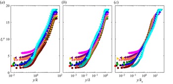
Figure 6 shows the mean streamwise velocity profiles normalised by different outer length scales for all the different rough surfaces used in this study. While for a given roughness geometry the corresponding profiles collapse regardless of the length scale used, the situation is different when we consider all roughness geometries together. Indeed, a lack of a general collapse is observed when the length scales  $k$ and
 $\delta$ are used, as shown in figures 6(a) and 6(b), respectively. This clearly indicates that the roughness height alone is not sufficient parameter to characterise the surface roughness. A similar remark has been made by Squire et al. (Reference Squire, Morrill-Winter, Hutchins, Schultz, Klewicki and Marusic2016) and Djenidi et al. (Reference Djenidi, Talluru and Antonia2018) who argued that an outer length scale cannot be used to collapse velocity profiles normalised by the inner velocity scale when considering different kinds of roughnesses. However, when the equivalent sand grain roughness
 $k_{s}$ is used the profiles appear to collapse better, as seen in figure 6(c). This suggests that, even though
 $k_{s}$ has no real physical meaning, it is nevertheless commonly used to characterise roughness. In that aspect, it is, from an engineering point of view, a very useful roughness length scale.. Unfortunately, its lack of physical meaning makes it impossible to measure it directly from the topology of the surface. Nevertheless, there are attempts to correlate this parameter with the actual roughness parameters (Schultz & Flack Reference Schultz and Flack2009; Flack et al. Reference Flack, Schultz and Barros2020). Unfortunately, none of these attempts provides a universal
 $k_{s}$ that can be used for all kinds of roughness geometries. This, however, does not preclude the possibility of proposing a
 $k_{s}$ that can be valid for a given family of a roughness geometries. In the next section we attempt to develop an expression for
 $k_{s}$ for 2-D roughness.
The streamwise mean velocity profiles over different rough surfaces at matched Reynolds number  $3300< Re_{\tau }<4300$ where each surface is normalised by the friction velocity
 $U_{\tau }$. The wall-normal position
 $y$ is normalised by different outer length scales. The symbols of the different rough surfaces are detailed in table 3. (a) The wall-normal position
 $y$ is normalised by the outer roughness length scale
 $k$. (b) The wall-normal position
 $y$ is normalised by the outer length scale
 $\delta$. (c) The wall-normal position
 $y$ is normalised by the outer roughness length scale
 $k_{s}$.

4.2.2. Roughness function
Roughness has a wide range of shapes, types and textures that makes it almost impossible to characterise it by a single physical roughness parameter. Firstly, we need to define, if possible, the major roughness parameters that mostly affect the drag. Then, develop an equation for the equivalent sand grain roughness  $k_{s}$ that combines these parameters. The most common roughness parameter used to characterise the roughness is its height. There are various heights that can be measured from the roughness topography such as the average roughness height
 $k_{a}$, the root-mean-square roughness height
 $k_{rms}$, the maximum peak to valley roughness height
 $k$ and the average of the highest 5 roughness peaks to the maximum lowest valleys
 $k_{z}$ (ASME 2009). However, none of these roughness height parameters are alone capable of describing the roughness completely.
Figure 7 shows  $\Delta U^{+}$ as a function of maximum peak-to-valley roughness height,
 $k$, for all the different surfaces used in this study. Each rough surface has different
 $\Delta U^{+}$ in the fully rough regime, and there is no corresponding map function between the roughness height and the roughness function. All the surfaces used in this study only have two maximum peak to valley heights, even though the wall drag changes from one surface to another. Hence, another family of roughness parameters must be employed.
Roughness function  $\Delta U^{+}$ as a function of maximum peak-to-valley roughness height,
 $k$, normalised by the inner length scale
 $\nu /U_{\tau }$. The filled symbols are the different surfaces roughness symbols indicated in table 3.

The frontal solidity  $\lambda _{f}$ is defined as the ratio of the total projected frontal area to the total plan area. This parameter indicates how big the area exposed to the flow is, which can be directly related to the pressure drag (MacDonald et al. Reference MacDonald, Chan, Chung, Hutchins and Ooi2016). Napoli et al. (Reference Napoli, Armenio and De Marchis2008) introduced the effective slope
 $ES$, defined as the mean absolute gradient of a roughness surface
 $ES=2\lambda _{f}$. The advantage of using
 $ES$ over
 $\lambda _{f}$ is that the gradient can be calculated for any surface, even for random roughnesses, which makes it more general and robust in characterising the roughness.
Figure 8 shows  $\Delta U^{+}$ as a function of
 $ES$. It can be seen that, for the rods,
 $\Delta U^{+}$ increases with
 $ES$. Note that the roughness function for triangular rib and sinewave surfaces is much lower than rods that have the same
 $ES$. This may be due to the fact that
 $k_{sk}=0$ for the former roughnesses. The data of Napoli et al. (Reference Napoli, Armenio and De Marchis2008), who carried out a large eddy simulation of a rough wall turbulence channel flow, are reported in figure 8. Their roughness consisted of corrugated walls covering a wide range of
 $ES$. We observe that our sinewave roughness functions match very well with their data. This validates the argument concerning the importance of the effective slope in determining the roughness function as well as in validating our measurements. The message of figure 8 is that, for a fixed
 $ES$, highly skewed surfaces, such as rods, have higher roughness functions than corrugated-like surfaces. Further information one can infer from the figure is that it is challenging to describe a surface with only one roughness parameter. This reinforces the idea that a combination of two or more roughness parameters is likely to be needed to adequately characterise roughnesses. Although roughness height and slope reveal most of the roughness characteristics, they are not sufficient to completely describe the roughness.
Roughness function  $\Delta U^{+}$ as a function of effective slope,
 $ES$. The filled symbols are the different surfaces roughness symbols indicated in table 3. The blue pentagram symbols are channel flow data over various irregularly distributed sinusoidal roughness from Napoli et al. (Reference Napoli, Armenio and De Marchis2008).

Figure 9 shows the streamwise mean velocity profiles over  $R16-08$,
 $S16-08$ and
 $T16-08$ surfaces. These three surfaces have the same roughness height,
 $k$, and the same effective slope,
 $ES$, but different geometries. The roughness functions,
 $\Delta U^{+}$, for
 $S16-08$ and
 $T16-08$ are almost the same, however, they have lower
 $\Delta U^{+}$ than
 $R16-08$.
The streamwise mean velocity profiles over three different roughnesses with the same height,  $k$, and effective slope,
 $ES$, but different geometries normalised by the friction velocity
 $U_{\tau }$. Cases
 $R16-08$,
 $S16-08$ and
 $T16-08$ are compared with the smooth TBL data from Marusic et al. (Reference Marusic, Chauhan, Kulandaivelu and Hutchins2015). The symbols of our different surfaces are indicated in table 3.

If we consider these roughnesses and consult table 1 we note that the skewness,  $k_{sk}$, of the sinewave and the triangular ribs is the same, but different from the rods. Hence, a third group of roughness parameters should be introduced to adequately describe the roughness.
The plan solidity,  $\lambda _{p}$, is defined as the ratio of the total projected plan area to the total plan area. This parameter measures how dense the roughness is (Placidi & Ganapathisubramani Reference Placidi and Ganapathisubramani2015). As mentioned above,
 $ES$ is more usable than
 $\lambda _{f}$ and can be used even for random roughness, the skewness of the roughness is more usable than the plan solidity and can be used for regular and irregular roughnesses. The skewness measures the symmetry of a profile about the mean line. It indicates a morphology of the surface texture;
 $k_{sk}>0$ corresponds to high peaks, while
 $k_{sk}<0$ corresponds to pitted surfaces.
Figure 10 shows  $\Delta U^{+}$ as a function of
 $k_{sk}$ in the fully rough regime. It can be noticed that, for the rods only, the roughness function decreases with increasing roughness skewness. The roughness functions for triangular rib and sinewave surfaces have lower values than rods, as they have zero roughness skewness value.
Roughness function  $\Delta U^{+}$ as a function of roughness skewness,
 $k_{sk}$. The filled symbols are the different surfaces roughness symbols indicated in table 3.

Attempts to correlate the  $k_{s}$ with roughness parameters like
 $k_{sk}$, and
 $k_{rms}$ have been carried out (see Flack et al. Reference Flack, Schultz, Barros and Kim2016). Others proposed to relate
 $\Delta U^{+}$ to
 $ES$ instead of
 $k_{s}$ (Napoli et al. Reference Napoli, Armenio and De Marchis2008). However, a review of these different proposals shows that they apply to particular roughness geometries. This raises an interesting practical issue concerning whether these roughness parameters can be related to
 $k_{s}$, which controls the roughness function
 $\Delta U^{+}$ as follows (Nikuradse Reference Nikuradse1933):
 \begin{equation} \Delta U^{+} =\frac{1}{\kappa}\log(k_{s}^{+})+B-8.5.\end{equation}
In the following analysis we use  $\kappa =0.405$ and
 $B=5$ and only data for which
 $\Delta U^{+}>8.5$ are used to compute
 $k_{s}^{+}$. It would seem that a combination of the three roughness parameters (
 $k$,
 $ES$ and
 $k_{sk}$ would provide a better correlation function for
 $k_{s}$.
Figure 11 suggests that the expression (4.2) provides a suitable empirical relation for  $k_{s}$ for 2-D roughness. It is thus of interest to assess how this relation compares with previous experimental and numerical results for
 $k_{s}$. This comparison is reported in figure 12, which shows the present predicted values of
 $k_{s}$ with those of Krogstad & Efros (Reference Krogstad and Efros2012), Djenidi et al. (Reference Djenidi, Talluru and Antonia2018) and Leonardi et al. (Reference Leonardi, Orlandi, Smalley, Djenidi and Antonia2003). In this figure, a perfect agreement between the present predictions and measurement is represented by a straight line. While there is some scatter in the data, the figure shows a clear trend: the data align relatively well with the straight line, providing support for (4.2)
 \begin{equation} {{k_{s} = a + b \times k + c \times \frac{2k}{ES} + d \times ES \times k_{sk}}}, \end{equation}
where  $a$ = 0.001,
 $b$ = 1.865,
 $c$ = -0.103,
 $d$ = 0.013, with
 $R^{2}$ = 0.93. here,
 $R^{2}$ is a statistical measure of how close the data are to the fitted regression line. It can be noticed that
 ${2k}/{ES}$ =
 $s_{x}$ for uniform distributed roughness. It can be observed that, when
 $k_{sk}=0$, as for sinewaves or triangular ribs,
 $k_{s}$ will depend only on the roughness height
 $k$ and the spacing between two consecutive roughness peaks
 $s_{x}$ for distributed 2-D roughness or the effective slope for random roughness. However, for highly positive skewed roughness like 2-D cylindrical rods, both
 $k_{sk}$ and
 $ES$ affect
 $k_{s}$ and are accounted for by the last term of (4.2). All data in the fully rough regime are on Nikuradse's asymptote line. These data support the proposal that
 $k_{s}$ correlates very well with the drag coefficient
 $\Delta U^{+}$ in the fully rough regime. Remarkably, a very good agreement is observed between
 $\Delta U^{+}$ obtained using the measured and predicted values of
 $k_{s}^{+}$, indicating that (4.2) provides a suitable equation for predicting
 $k_{s}$ for a family of 2-D rough surfaces, i.e. 2-D cylindrical rod roughnesses and 2-D sinewaves or triangular ribs. This linear equation is developed for uniform 2-D roughnesses with
 $ES$ varying from 0.08 to 0.33 and positive skewness roughness
 $0 \leq k_{Sk} \leq 4.7$.
The roughness function for 2-D roughness as a function of equivalent sand grain roughness height  $k_{s}$, normalised by the inner length scale
 $\nu /U_{\tau }$. The filled symbols are the different surface roughness symbols indicated in table 3. The unfilled symbols are the predicted
 $k_{s}^{+}$ values from (4.2) for the same rough surface. The black solid line is the fully rough asymptote of Nikuradse (Reference Nikuradse1933). The values of
 $k_{s}$ of Krogstad & Antonia (Reference Krogstad and Antonia1999), Kamruzzaman et al. (Reference Kamruzzaman, Djenidi, Antonia and Talluru2015) and Djenidi et al. (Reference Djenidi, Talluru and Antonia2018) are reported in the figure for comparison and validation.

Comparison between actual  $k_{s}$ measured from mean velocity profiles and the calculated
 $k_{s}$ from (4.2) for our surfaces along with previous experimental and numerical results for 2-D roughness only.

Since this empirical relation (4.2) has been developed for 2-D roughness, it was observed that it was not valid for 3-D roughness. Instead, a new empirical relation was developed for the 3-D roughness. Using the data of Flack et al. (Reference Flack, Schultz and Barros2020), Barros, Schultz & Flack (Reference Barros, Schultz and Flack2018), Busse, Thakkar & Sandham (Reference Busse, Thakkar and Sandham2017), Forooghi et al. (Reference Forooghi, Stroh, Magagnato, Jakirlić and Frohnapfel2017) and Squire et al. (Reference Squire, Morrill-Winter, Hutchins, Schultz, Klewicki and Marusic2016) and the same physical roughness parameters used for 2-D roughness ( $k$,
 $k_{sk}$ and
 $ES$), we obtained the following empirical relation:
 \begin{equation} {{k_{s} = a + b \times k + c \times k_{sk} + d \times \frac{2k}{ES} + e \times ES \times k_{sk}}}, \end{equation}
where  $a = -0.000025$,
 $b = 1.654$,
 $c = 0.004$,
 $d = -0.2$,
 $e = -0.0009$ with
 $R^{2}=0.79$. Notice the addition of a fifth term. Figure 13 compares the prediction of
 $k_{s}$ using (4.3) with the values of
 $k_{s}$ for the same data used to develop (4.3). While the data tend to exhibit an alignment with the straight line, there is a stronger scatter than in figure 12, as quantified by a lower value of
 $R^{2}$. The fact that two separate relations are required for the 2-D and 3-D roughnesses suggests that it is unlikely that one can develop a truly universal relation for
 $k_{s}$. We nevertheless attempted to obtain an empirical relation for both the 2-D and 3-D data. The result was the following relation:
 \begin{equation} {{k_{s} = a + b \times k + c \times \frac{2k}{ES} + d \times {\frac{2k}{ES}}^{2} + e \times {\rm e}^{f \times ES \times k_{sk}}}},\end{equation}
where  $a = -0.002$,
 $b = 0.926$,
 $c = 0.283$,
 $d = 4.933$,
 $e = 0.001$,
 $f = 3.66$, with
 $R^{2}=0.87$.
Comparison between actual  $k_{s}$ from the literature and the calculated
 $k_{s}$ from (4.3) for 3-D roughness only.

Notice that, conversely to the two previous relations, (4.4) is nonlinear; it was not possible to obtain a linear function that yields a reasonable fit to the data. Figure 14 shows the comparison between the predicted values of  $k_{s}$ with the measured ones. The data exhibit a large scatter around the straight line, even though the data show a tendency to align with that line, particularly the 2-D rough wall data.
Comparison between actual  $k_{s}$ and the calculated
 $k_{s}$ from (4.4) for 2-D and 3-D roughnesses.

It is important to stress that, like  $k_{s}$ itself, empirical relations like (4.2), (4.3) and (4.4) bear no physical meaning. However, their relevance and usefulness, from an engineering viewpoint, lie in the fact that they relate physical quantities for characterising the roughness geometry. Thus, the ability to predict
 $k_{s}$, which can be related to the drag, using simply the roughness parameters has an obvious practical interest.
More experiments for various kinds of roughnesses (2-D roughness such as grooves instead of rods to include negative skewness roughness as well as 3-D sinusoidal and random roughnesses) are needed to either validate and/or improve the previous expressions and to determine whether a universal formula for  $k_{s}$ can be developed for all kinds of roughness geometries.
5. Conclusions
Measurements are performed in a ZPG rough wall TBL to investigate the effect of different roughness parameters. Single hot-wire probes are used to measure the streamwise velocity at various Reynolds numbers and for 2-D roughness geometries. Circular rods with two different heights,  $k= 1.6$ and 2.4 mm, and five different streamwise spacing ratios ranging from 6 to 24, 3D printed triangular ribs with heights of
 $k= 1.6$ mm and a spacing of
 $8k$ and CNC machined sinewave surfaces with two different heights,
 $k= 1.6$ and 2.4 mm, and a spacing ratio of 8 were investigated. These surface roughnesses covered a wide range of
 $\delta /k$ ranging from 23 to 41 in the fully rough regime.
The roughness causes a downward shift of the wall-unit normalised mean velocity profile, known as the roughness function. The maximum downward shift is reached when the spacing ratio between two roughness elements is approximately 8. Changing the roughness height, while maintaining the same spacing ratio, does not affect the drag coefficient in the fully rough regime. Varying  $\delta /k$ does not affect the mean streamwise velocity profile, if
 $\delta /k$ is large enough;
 $\delta /k>23$ in this study. This reveals that roughness height is not an appropriate parameter to characterise the roughness.
An excellent collapse of the log region in the mean velocity profiles is observed when the equivalent roughness length scale  $k _{s}$ is used as a length scale to normalise the mean velocity profiles. Further, while
 $k_{s}$ is not an actual physical roughness parameter that can be measured directly from the topology of the surface, a new expression for
 $k_{s}$ involving the physical roughness parameters
 $k$,
 $ES$ and
 $k_{sk}$ is proposed. It is shown that this new empirical relation provides a promising practical means to calculate the roughness function directly from the roughness topography in 2-D uniformly distributed rough surfaces. The relation shows that
 $k$,
 $ES$ and
 $k_{sk}$ are major surface roughness parameters affecting the turbulence statistics and drag coefficient.
Our results indicate that such general scaling cannot exist because of the complexity of the roughness geometries which involve too the many parameters. Further, the results suggest it is likely each family of roughnesses (for example 2-D roughness, 3-D roughness) would have its own scaling.
It should be noted that this new relation for  $k_{s}$ is limited to 2-D uniformly distributed roughness in a fully rough regime and more experiments on 2-D and 3-D rough surfaces, as well as random roughness, are needed to assess the importance of
 $k$,
 $ES$ and
 $k_{sk}$ in the turbulence statistics and drag coefficient. Such studies will help develop a more generalised relation for
 $k_{s}$, if such a generalisation can be made.
Funding
The authors acknowledge the financial support of the Australian Research Council.
Declaration of interests
The authors report no conflict of interest.