INTRODUCTION
The common dolphinfish (Coryphaena hippurus Linnaeus, 1758) is a widely distributed and abundant epipelagic predator. This species is reported from 46°N to 38°S worldwide (Palko et al., Reference Palko, Beardsley and Richards1982; Norton, Reference Norton1999). It is caught in oceanic, coastal and estuarine waters, and its distribution is restricted mainly to waters less than 30 m deep and over 20°C (Kojima, Reference Kojima1966; Palko et al., Reference Palko, Beardsley and Richards1982). Common dolphinfish are caught in several regions of the world, and are important in commercial and sport fisheries (Palko et al., Reference Palko, Beardsley and Richards1982). In Mexico, this species is in high demand for sport and coastal fisheries, especially in the Pacific Ocean (Aguilar-Palomino et al., Reference Aguilar-Palomino, Galván-Magaña, Abitia-Cardenas, Muhlia-Melo and Rodriguez-Romero1998, Zúñiga-Flores et al., Reference Zúñiga-Flores, Ortega-Garcia and Klett-Traulsen2008).
Diet and feeding habit studies are important to understand the function of species in ecosystems. Studies on the feeding habits of common dolphinfish in several parts of the world have revealed that this species feeds mainly on fishes, followed by cephalopods and crustaceans (Tester & Nakamura, Reference Tester and Nakamura1957; Rothschild, Reference Rothschild1964; Rose & Hassler, Reference Rose and Hassler1974; Manooch et al., Reference Manooch, Mason and Nelson1983; Oxenford & Hunte, Reference Oxenford and Hunte1999).
Several studies have been carried out in the eastern Pacific Ocean on the feeding habits of this species, such as those by Hida (Reference Hida1973), Saucedo-Barrón (Reference Saucedo-Barrón1990), Campos et al. (Reference Campos, Segura, Lizano and Madrigal1993), Aguilar-Palomino et al. (Reference Aguilar-Palomino, Galván-Magaña, Abitia-Cardenas, Muhlia-Melo and Rodriguez-Romero1998), Lasso & Zapata (Reference Lasso and Zapata1999), Olson & Galván-Magaña (Reference Olson and Galván-Magaña2002), and Velasco-Tarelo (Reference Velasco-Tarelo2003). These authors found that common dolphinfish are mainly piscivorous generalists.
All these earlier studies used stomach content analysis to describe diet; however, a technique that uses the accumulation of stable isotopes in animal tissues to describe their trophic ecology has recently become widely used (Minagawa & Wada, Reference Minagawa and Wada1984). The stable isotope technique gives information on long-term feeding (depending on the tissue used), whereas stomach contents only provide short-term information of prey consumed at a given moment (Gearing, Reference Gearing, Coleman and Fry1991). The most common isotopes used for trophic analyses are carbon (C) and nitrogen (N). Analysis of 15N isotopes provides information on the trophic level of the predator, while 13C isotopes analysis can trace the origin of the carbon through the trophic web (Clarke et al., Reference Clarke, Vidergar and Bennett2005). We used stable isotope analysis to describe the trophic ecology (Minagawa & Wada, Reference Minagawa and Wada1984) of dolphinfish.
Further, we used previously published data on stomach contents of dolphinfish in Mazatlán to compare the diet composition between two areas in the southern Gulf of California (Tripp-Valdez et al., Reference Tripp-Valdez, Galván-Magaña and Ortega-García2010).
MATERIALS AND METHODS
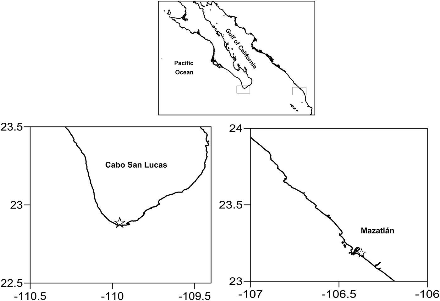
Common dolphinfish were collected from the sport fishery of Cabo San Lucas (CSL) and from the artisanal fishing fleet of Mazatlán, during the years 2000, 2001 and 2003. Cabo San Lucas is located at 22°45′00″N and 109°30′00″W (Figure 1). The sport fishing fleet in this area operates 20 to 30 nm from the coastline, trolling with rods or hand lines, with a lure or with live bait (mainly jack mackerel Scomber japonicus). Mazatlán is located at 23°04′25″N and 106°37′10″W; the artisanal fleets in Mazatlán operate in a similar manner to those of CSL, using hand lines.
Study area off the Baja California Peninsula in the Southern Gulf of California.

Specimens collected were measured (fork length FL in cm), sex was determined, and stomachs were collected and preserved frozen. Data on stomach content from the Mazatlán area were obtained from the database used by Tripp-Valdez et al. (Reference Tripp-Valdez, Galván-Magaña and Ortega-García2010). Samples from the dorsal muscle region of dolphinfish were collected in 2003 when available. Muscle samples from selected prey species that were part of stomach contents and were in a minimal state of digestion were also collected for stable isotope analysis.
Stomach contents analysis
In the laboratory, prey items were identified to the lowest possible taxon, using specialized keys (Clothier, Reference Clothier1950; Iverson & Pinkas, Reference Iverson and Pinkas1971; Miller & Lea, Reference Miller and Lea1972; Wolff, Reference Wolff1984; Clarke, Reference Clarke1986; Allen & Robertson, Reference Allen and Robertson1994; Fischer et al., Reference Fischer, Krupp, Schneider, Sommer and Carpenter1995; Thomson et al., Reference Thomson, Findley and Kerstich2000). Prey items were counted (N) and weighed (W in g), and the frequency of occurrence (FO) was recorded (Hyslop, Reference Hyslop1980). These measures were used because they are important in ecosystem models and comparative diet studies (Preti et al., Reference Preti, Smith and Ramon2004).
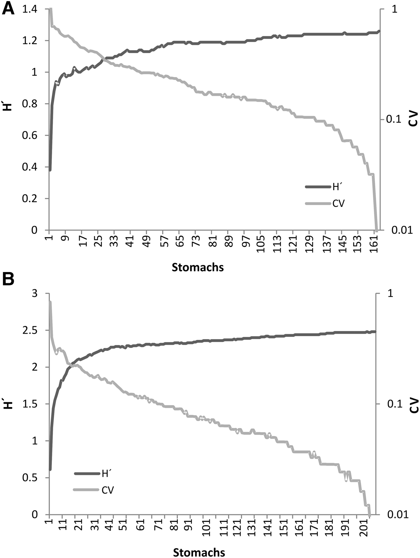
To determine whether the analysed sample number was sufficient to accurately represent the common dolphinfish diet, we did a randomized cumulative Shannon diversity curve using the software EstimateS v8 and calculated the coefficient of variation (CV) of these values. When an asymptotic stabilization of the curve was obtained (Cortés, Reference Cortés1997) and a CV value below 0.05 was achieved, we considered that the minimum number of stomachs required to accurately describe the diet had been reached.
The N, W and FO values were combined to calculate the geometric importance index (GII) proposed by Assis (Reference Assis1996). This index was calculated using the following equation:
 $${\bf GII}_{\bf j} = \displaystyle{{\left({\mathop {\bf \Sigma} \nolimits_{{\bf i} = 1}^{\bf n} {\bf Vi}} \right)_{\bf j} } \over {\sqrt {\bf n} }}$$
Where GIIj is the value of the index of geometric importance for the jth prey category, Vi is the sum of the percentages of the N, W and FO indices, and n is the number of indices used, in this case 3. This index measures prey importance as a distinct orthogonal vector; it combines the different index values into a resultant vector, and then solves for its components along a reference diagonal that represents maximum prey utilization. From the resulting geometry, the GII can be related directly to the degree of feeding specialization on a particular prey type (Assis, Reference Assis1996; Preti et al., Reference Preti, Smith and Ramon2001).
To determine differences in the diet of dolphinfish of different lengths, we grouped the specimens into three size classes: small (40–80 cm FL), medium (80–100 cm FL) and large (>100 cm FL) for analysis of size-related changes in diet. These size classes were chosen in such a way that all sizes were well represented based on the size distribution of dolphinfish in both areas.
In order to determine whether there were differences in diet between sexes or size classes, similarity was analysed using permutation-randomization methods in a Bray–Curtis dissimilarity matrix (ANOSIM, PRIMER 6 v. 6.1.6). The global rank dissimilarity R (0 ≤ R ≤ 1) is a useful comparative measure of the degree of separation. When R is near zero, Ho cannot be rejected; i.e. there is no separation between groups (Clarke & Warwick, Reference Clarke and Warwick2001).
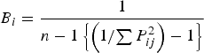
The degree of selectivity of the common dolphinfish diet was determined using Levińs standardized index (Krebs, Reference Krebs1999):
 $$B_i = \displaystyle{1 \over {n - 1\left\{{\left({{1 / {\sum {P_{ij}^2 } }}} \right)- 1} \right\}}}$$
Where B i is the trophic niche amplitude, ∑Pij is the proportion of the diet of predator i that includes prey j, and n is the total number of prey species. This index ranges from 0 to 1; values close to 0 (<0.6) indicate that the predator is selecting some prey groups; values close to 1 (>0.6) indicate that the predator is a generalist (Krebs, Reference Krebs1999).
The trophic level (TL) of common dolphinfish in the study area was determined using the TrophLab routine (available from www.fishbase.org) developed by Pauly et al. (Reference Pauly, Christensen, Froese and Palomares2000), using the biomass of each principal prey group, as well as the trophic level of each prey. The prey trophic levels were obtained from the Fishbase database (http://www.fishbase.org) and SeaLifebase database (http://www.sealifebase.org).
In order to estimate seasonal changes in the dolphinfish diet we calculated the monthly sea surface temperature of the study area using AVHRR satellite images (4 km resolution) obtained from NOAA (http://www.nodc.noaa.gov/SatelliteData/pathfinder4km/available.html).
Using this information we defined a cold season from December to June, and a warm season from July to November.
Stable isotope analysis
Samples of common dolphinfish muscle and their main prey were lyophilized to eliminate humidity. Since lipids are depleted in δ13C relative to proteins and carbohydrates, and variation in lipid contents among organisms or among tissue types would introduce considerable bias in stable isotope analyses that use δ13C (Post et al., Reference Post, Layman, Arrington, Takimoto, Quattrochi and Montana2007), lipids were extracted using a MARS-5 microwave oven (CEM Corp., Matthews, NC), which is a fast and efficient method to extract lipids (Paré et al., Reference Paré, Bélanger and Stafford1994; Renoe, Reference Renoe1994).
Samples were homogenized to a fine powder using an agate mortar. Stable isotope analysis was carried out using an isotope ratio mass spectrometer (IRMS) (20–20 mass spectrometer, PDZ Europa, Sanback, UK). Results are expressed as δ values in ‰ deviation from international standards, using the following equation (Park & Epstein, Reference Park and Epstein1961):
 $$\delta ^{ 15} {\rm N}\, \, {\rm or}\, \, \delta ^{ 13} {\rm C} = [\lpar R_{{\rm sample}} /R_{{\rm standard}} \rpar - 1] \times 1000$$
R = 13C/12C or 15N/14N respectively
Standard = atmospheric nitrogen for N and Pee Dee Belemnite for C.
Isotopic values of common dolphinfish and their prey were included into a mixing model, using the SISUS software (Erhardt, Reference Erhardt2007; www.statacumen.com/sisus/) to convert the isotopic values to values representing the relative contribution of the food type to the diet.
The model applies a Bayesian approach that uses values of carbon and nitrogen isotopes to calculate the most probable contribution of the different sources (prey) to the mix (predator). The results of this analysis are distributions of the importance of each item to the diet in percentage values, which range from 1 to 99%.
Prior to the analysis, we corrected the isotopic fractionation (enrichment) value of the predator by subtracting 2.4‰ from the average isotopic signal of common dolphinfish. This value was calculated by obtaining the average value of the isotopic difference between δ15N values of the predator and each prey type (Kelly et al., Reference Kelly, Robertson, Murphy, Fitzsimons, Costello, Gormley, Corner and Marples2012) in both areas.
The common dolphinfish trophic level was estimated from the isotopic values using the equation proposed by Post (Reference Post2002).
 $$TL_{{\rm isotope}} = \lambda + \displaystyle{{\lpar \delta ^{15} {\rm N}_{{\rm Predator}} - \delta ^{15} {\rm N}_{{\rm Base}} } \over {{\rm \Delta }_n }}$$
where δ15NPredator is the N isotopic composition of dolphinfish, λ is the trophic level of the organism used to estimate the N isotopic composition of the food base (δ15NBase), and Δn represents trophic enrichment (Post, Reference Post2002). For CSL the base prey used was Pleuroncodes planipes, which has a trophic level (TL) of 2.85, according to the Fishbase database (www.fishbase.org). For Mazatlán we used Exocoetus volitans as base prey, which has a TL of 3 according to Fishbase. For both zones we used an enrichment value of 2.4‰.
We tested differences in the diet between the different zones, size classes, seasons and sexes. We applied a multivariate analysis of variance (MANOVA) in R (R Development Core Team, 2011) version 2.14.1, using the vegan package for both stomach contents and isotopic values.
RESULTS
Stomach contents
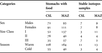
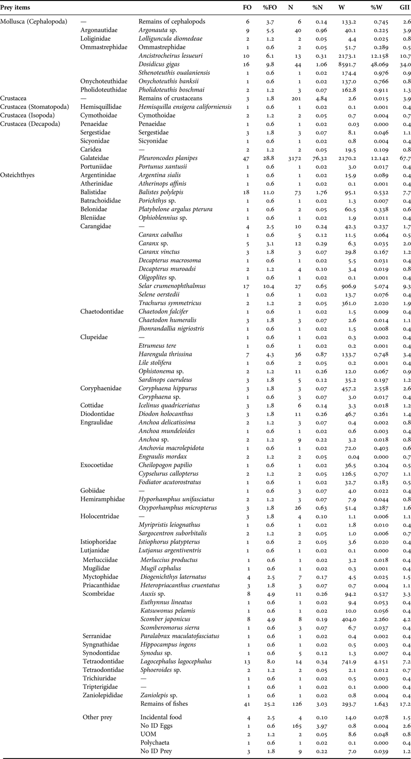
A total of 215 stomachs were collected from CSL (Table 1). Sizes of dolphinfish ranged from 47 to 141 cm fork length, with an average size of 90 cm. Of 215 stomachs analysed, 76% contained food. The trophic spectrum comprised 86 prey items, of which 63 were fishes, nine were crustaceans, nine were molluscs (cephalopods) and the rest was unidentified organic matter (UOM) (Table 2).
Accumulated diversity curve for both areas, showing that the diet is well represented where the curve becomes asymptotic and the CV reaches a value under the 0.05. A = Cabo San Lucas, B = Mazatlán.
Number of samples by category for stomach contents and stable isotope samples
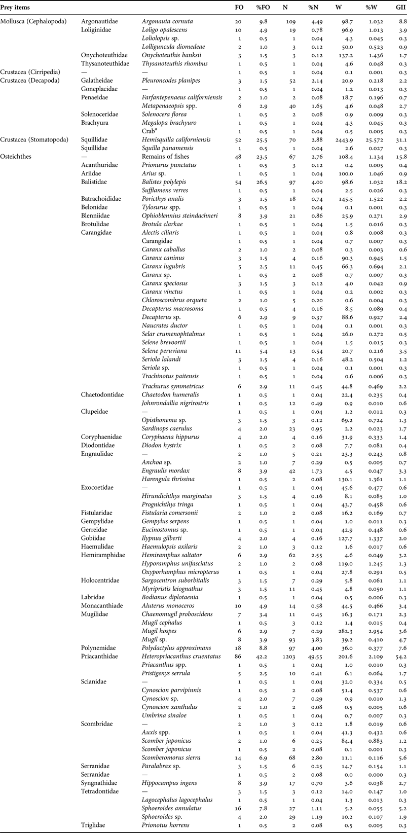
Composition of stomach contents from dolphinfish Coryphaena hippurus collected in Mazatlán expressed as absolute and percentage values of the frequency of occurrence (FO), numeric (N), weight (W) and GII indexes.
aNo identified specimens.
A total of 230 stomachs were collected in Mazatlán (89% of them containing food). The size of dolphinfish ranged from 45 to 153 cm fork length, with an average of 77 cm. The trophic spectrum was composed of 98 prey items: 79 fishes, 10 crustaceans, seven molluscs, and UOM (Table 3). For both areas the number of analysed stomachs was deemed to be sufficient because the cumulative diversity curve reached an asymptote, and the CV was below 0.05 (Figure 2).
Composition of stomach contents from dolphinfish Coryphaena hippurus collected in Cabo San Lucas expressed as absolute and percentage values of the frequency of occurrence (FO), numeric (N), weight (W) and GII indexes.
The MANOVA test showed significant multivariate effects of presence and biomass (W) of prey, which were attributed to season, area and size class (F (1,294) = 7.35, 15.88, 4.39, P = <0.001). There was no significant effect due to sex F (1,294), P = 0.747. The species variability was explained by the season (2%), the area (5%) and the size class (1.4%).
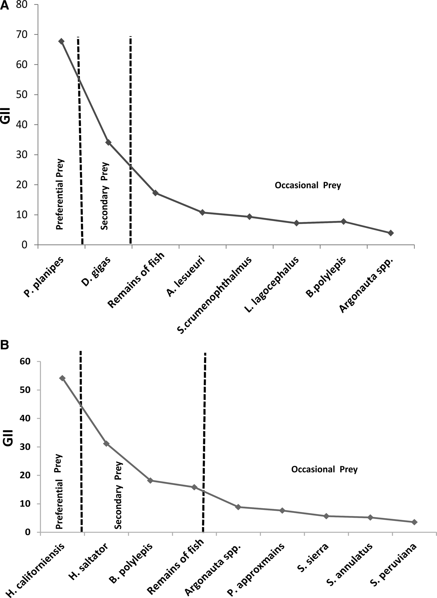
In the CSL area, the geometric importance index (GII) indicated that P. planipes (GII = 67.7) was the most important prey, followed by the jumbo squid Dosidicus gigas (GII = 34). The remaining species were classified as secondary or rare prey (Figure 3, Table 2). In the Mazatlán area the GII indicated that the crustacean Hemisquilla californiensis (GII = 54) was the main prey, followed by the fish Hemiramphus saltator (GII = 31), the triggerfish Balistes polylepis (GII = 18) and fish remains (GII = 16). The remaining prey species were classified as secondary or rare prey (Figure 3, Table 3).
Values of the geometric importance index, GIl, for all fish analysed in both areas. Vertical lines separate preferential or primary prey from the secondary or occasional prey. A = Cabo San Lucas, B = Mazatlán.
The diet was very similar for both sexes. The ANOSIM showed no diet separation between sexes. For CSL R ANOSIM = 0.013 with P = 0.07, and for Mazatlán R ANOSIM = 0.005 with P = 0.231.
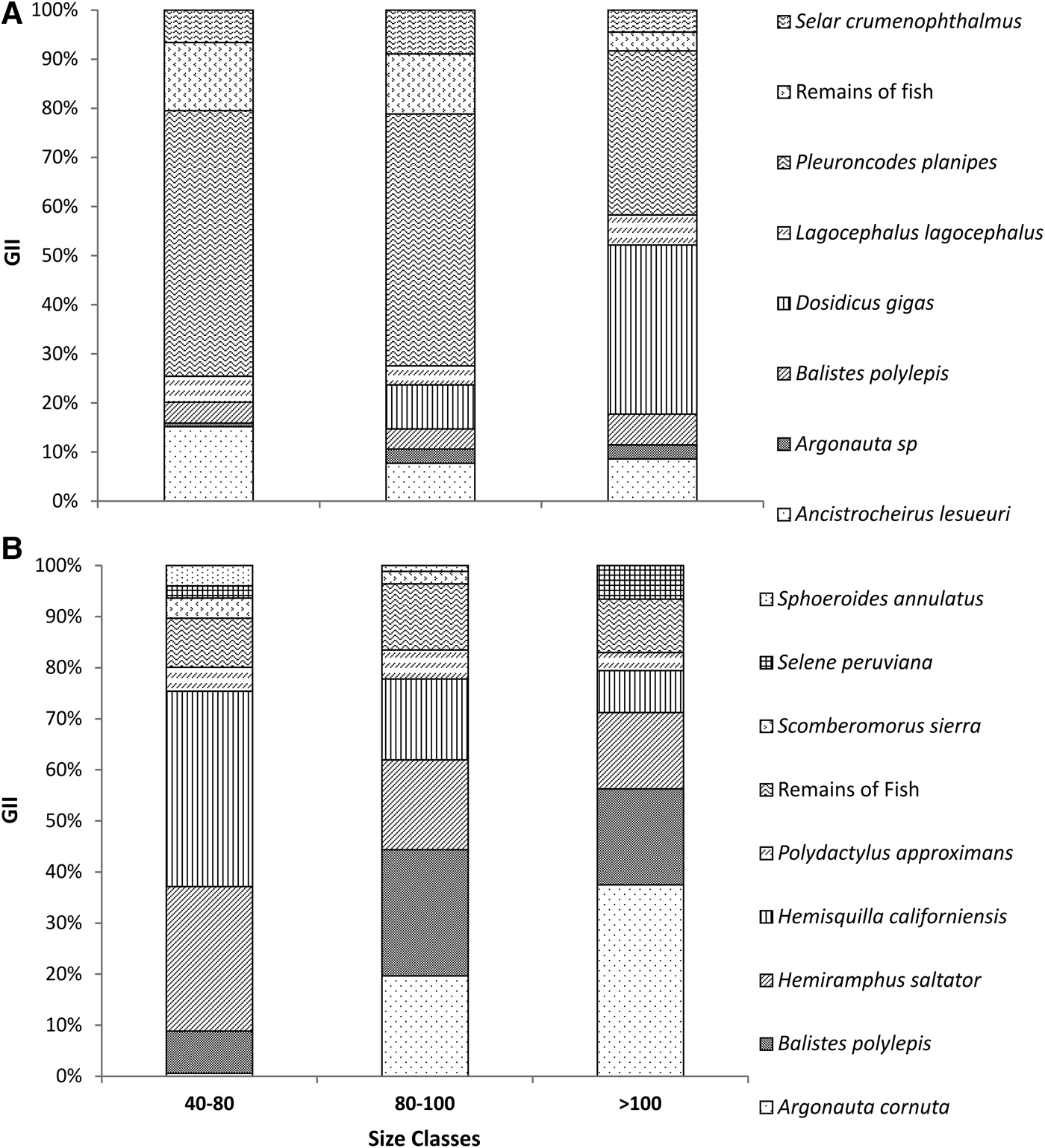
Three size intervals were defined: 40–80 cm, 80–100 cm and >100 cm fork length. For CSL, we found that there was no separation in the diet of the first two size classes (R ANOSIM = 0.005, P = 0.622), indicating that they were using the same prey in very similar proportions (Figure 4A). A comparison with the third size interval showed that there was a separation in the diet (R ANOSIM = 0.86, P = 0.001); for this size class cephalopods had a higher importance than for the previous two size classes (Figure 4). For Mazatlán we found significant differences for each size class (R ANOSIM = 0.168, P = 0.001), because the consumption of prey like cephalopods and fish seems to increase with size, and there is a reduction in the consumption of crustaceans in the larger fishes (Figure 4B).
Main dolphinfish prey species by size, expressed as % GII, as determined from samples taken during 2000, 2001 and 2003. A = Cabo San Lucas, B = Mazatlán.
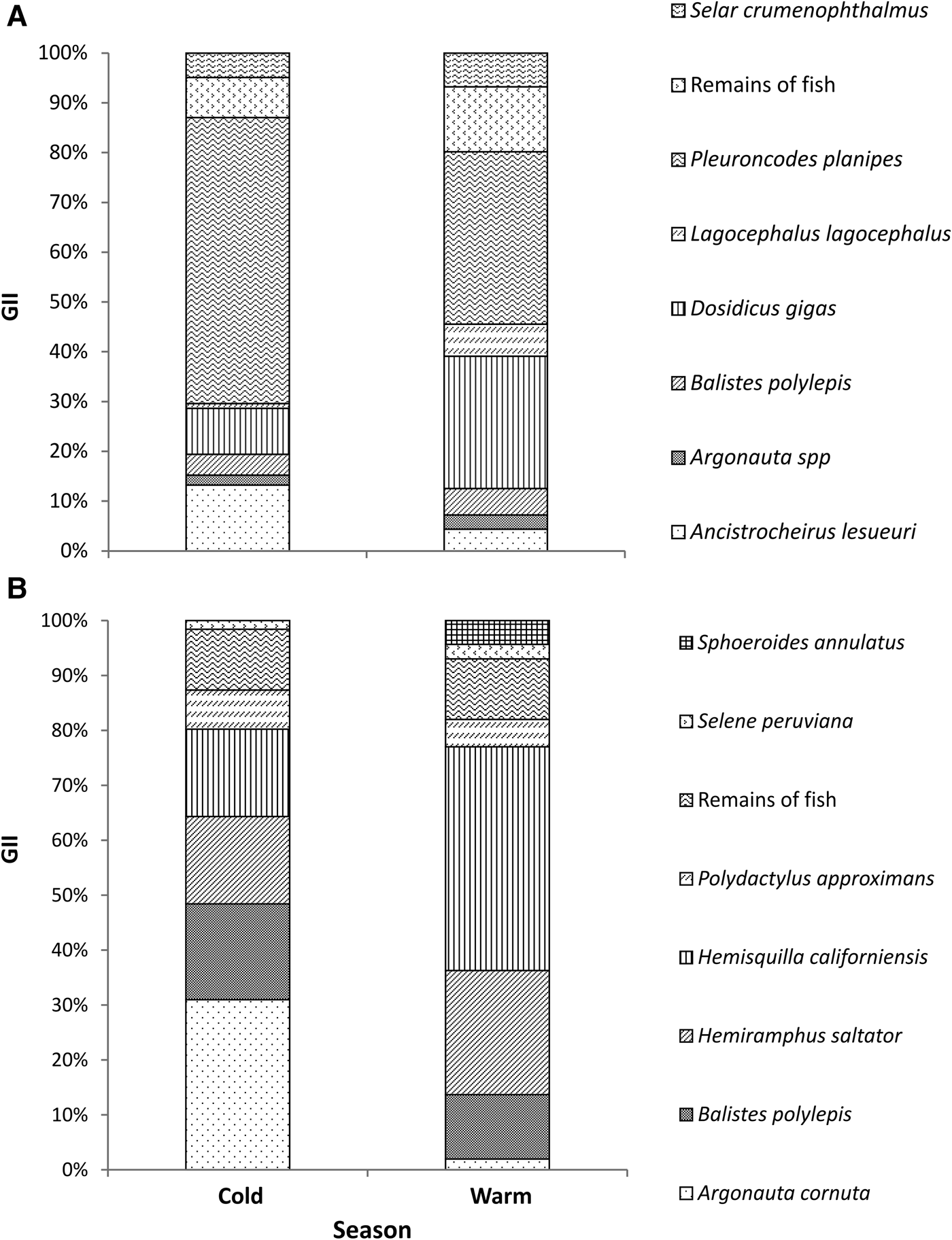
We found differences between the two seasons in both areas. In the CSL area (R ANOSIM = 0.032, P = 0.026) P. planipes had a higher importance during the cold season (GII = 95.27), than the warm season (GII = 52.84) (Figure 5A). In Mazatlán (R ANOSIM = 0.149, P = 0.001) the crustacean H. californiensis (GII= 60) was important during the warm season, while cephalopods (GII = 37) and fishes (GII = 20) were important during the cold season (Figure 5B).
Dolphinfish diet comparison between cold and warm seasons based on % GIl, A = Cabo San Lucas, B = Mazatlán.
The trophic level estimated for common dolphinfish in CSL was 4.34 (SE = 0.35); while in Mazatlán the estimated TL was 4.4 (SE = 0.33). The trophic niche width index (Levin's index) gave low values for both areas (B i < 0.03); which means that in spite of having a wide trophic spectrum this predator's diet was dominated by a few prey groups.
Stable isotopes analysis
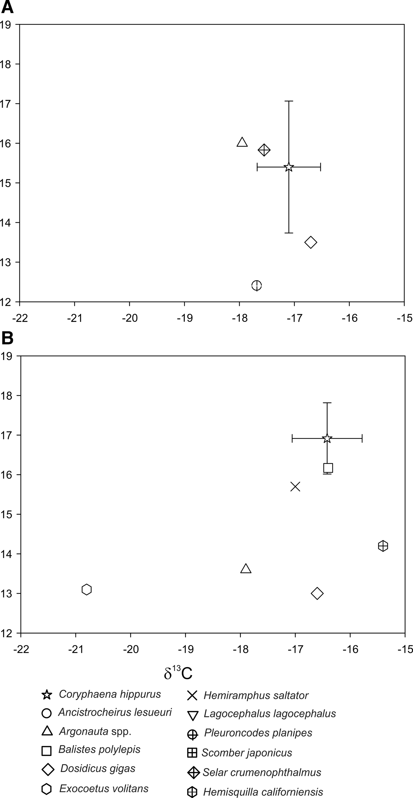
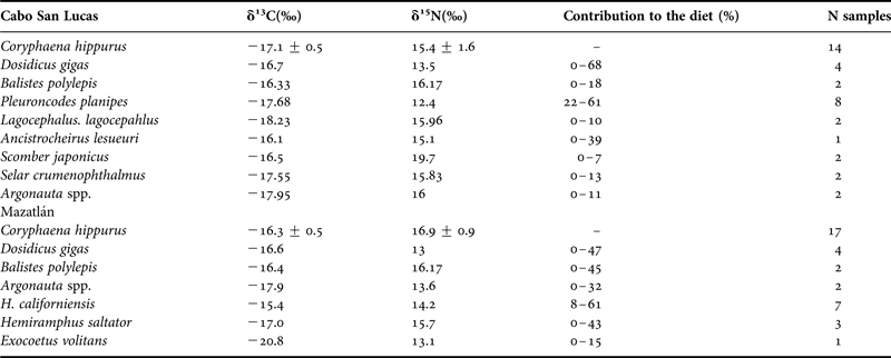
We collected 14 common dolphinfish muscle samples from CSL and 17 from Mazatlán, of all sexes, sizes and seasons. δ15N values ranged from 12.89 to 17.77‰, while δ13C values ranged from −18.07 to −15.13‰ (Figure 6). The MANOVA test showed significant differences in C and N isotope values between the two areas (F (1,26) = 16.10, P = 0.001).
Carbon and nitrogen isotope signatures of C. hippurus and its prey in Cabo San Lucas (A) and Mazatlán (B).
Mixing models using isotopic values from prey items previously identified as important in stomach content analysis showed that the jumbo squid D. gigas was the most important prey in CSL, contributing from 0 to 68% to the diet, followed by the crustacean P. planipes (22–61%), and the squid Ancistrocheirus lesueuri (0–39%). For Mazatlán the main prey were H. californiensis (0–61%), followed by D. gigas (0–47%), B. polylepis (0–45%), and H. saltator (0–43%). The remaining species were secondary (Table 4).
Isotopic values of Coryphaena hippurus and its potential prey, and their per cent contribution to the diet obtained from mixing models for both areas (Cabo San Lucas and Mazatlan).
The calculated trophic level (TL) using the method proposed by Post (Reference Post2002) was 4.4 (SE = 0.62) in CSL; in Mazatlán TL was 4.6 (SE = 0.37). These values were very similar to those obtained using stomach content analysis, and similar to the 4.37 value reported by Fishbase. The standard deviation (SD) of δ15N data was relatively low for Mazatlán (SD 0.9) and CSL (SD 1.2), suggesting low variability in the diet.
DISCUSSION
The results obtained with stomach content analysis corroborate previous findings that catalogued dolphinfish as a voracious predator with a wide trophic spectrum, feeding on fishes, cephalopods and crustaceans (Palko et al., Reference Palko, Beardsley and Richards1982). However, in this study, using both stomach content and stable isotope analyses, we found that three invertebrate species (D. gigas, P. planipes and H. californiensis) were the most important prey for dolphinfish, which contrasts with results from other authors such as Gibbs & Collete (Reference Gibbs and Collete1959), Rose & Hassler (Reference Rose and Hassler1974) and Manooch et al. (Reference Manooch, Mason and Nelson1983), who found that this species was mainly piscivorous.
We found different prey species in the two areas. This was probably due to the CSL area having a very narrow continental shelf compared with Mazatlán (Alvarez-Borrego, Reference Alvarez-Borrego and Ketchum1983), which resulted in the prey species found in CSL being more related to the pelagic zone. This was the case of P. planipes, and of some cephalopod and fish species that are usually pelagic. Balistes polylepis which is categorized as demersal was found only in its pelagic juvenile stage (Eschmeyer et al., Reference Eschmeyer, Herald and Hammann1983).
This type of prey was also found in 2005–2007 by Torres-Rojas et al. (Reference Torres-Rojas, Hernández-Herrera, Ortega-García and Soto-Jiménez2014) in this area, which indicates that this tendency is maintained over time. In Mazatlán we found more demersal prey, such as the crustacean H. californiensis, which in its megalops stage migrates from the bottom to the surface to feed (Salgado-Barragan, personal communication). We also found some fishes and pelagic prey such as squids and Argonauta spp.
Dolphinfish have opportunistic feeding habits, preying on the most abundant prey species in the environment. In the same study area of CSL in 1990 and 1991, Aguilar-Palomino et al. (Reference Aguilar-Palomino, Galván-Magaña, Abitia-Cardenas, Muhlia-Melo and Rodriguez-Romero1998) found that P. planipes and D. gigas were present in the diet of common dolphinfish. However, the fish B. polylepis, Auxis spp. and Cypselurus callopterus were more important in the diet, which suggests that in those years those fish species were more abundant.
This could be due to the sea surface temperature having reached higher levels in 1990 and 1991. This increase in temperature may have affected the distribution of P. planipes, which are associated with colder waters such as the California Current (Aurioles-Gamboa, Reference Aurioles-Gamboa, Aurioles-Gamboa and Balart1995). In those years there was a greater abundance of fish in the diet of dolphinfish, while in 2001 and 2003 with the presence of colder waters this crustacean became a more abundant prey of this predator.
Dosidicus gigas is found year round in the Gulf of California; its abundance changes in each area of the Gulf depending on the season, being less abundant during winter (Ehrhardt et al., Reference Ehrhardt, Solís, Jacquemin, Ortiz, Ulloa, González and García1986). However, it seems that variation in D. gigas abundance is not what determines dolphinfish diet; the feeding differences found with stomach content analysis during the warm and cold seasons in CSL could correspond to a higher abundance of P. planipes during the cold season rather than to a decrease in D. gigas abundance.
We detected a change in the dolphinfish diet in Mazatlán during the cold season that is related with an increase in the consumption of Argonauta spp. This increase could be a result of transport towards the coast during the cold season by currents or by the wind, caused by the presence of a shell that is formed to hold this organism's eggs (Laptikhovsky & Salman, Reference Laptikhovsky and Salman2003). However, the isotopic analysis did not show significant differences between seasons, suggesting that this increase in the consumption of Argonauta spp. was not enough to change the isotopic composition of the dolphinfish tissues.
We found differences in the diet among sizes using stomach content analysis in both areas. Larger and more mobile organisms are capable of catching a high biomass of fast prey, such as squid and fish (Olson & Galván-Magaña, Reference Olson and Galván-Magaña2002). However, stable isotope analysis showed few differences between dolphinfish of different sizes, which suggests that in spite of differences, found using stomach content analysis, the highly abundant P. planipes (Aurioles-Gamboa, Reference Aurioles-Gamboa, Aurioles-Gamboa and Balart1995) seems to be assimilated in a higher proportion by all size classes of dolphinfish.
This suggests that this prey is consumed frequently by the predator, despite some other prey being consumed occasionally in higher proportion. Pleuroncodes planipes seems to always be a complementary food due to its abundance, and this is reflected over the long term in the isotope signature found in the muscle tissue. In Mazatlán the same situation seems to happen with H. californiensis, which results in the isotopic signal for all size classes being very similar.
We could not find differences in diet between common dolphinfish males and females in the southern Gulf of California. There exist only two previous reports by Rose & Hassler (Reference Rose and Hassler1974) and Varghese et al. (Reference Varghese, Somvanshi, John and Dalvi2013), where the first authors found that males were more piscivorous than females and the second authors found a higher fish intake in females, which they suggest is due to higher energy requirements for reproduction. In our study males and females consumed the same prey at almost the same rate.
Stomach content and stable isotope analyses showed that although this predator consumed a broad prey spectrum, only a few prey items made up the bulk of the diet. This was mainly reflected in the low SD of δ15N values and low Levin's index values. We consider that dolphinfish are opportunistic predators that may consume diverse prey (Palko et al., Reference Palko, Beardsley and Richards1982), although they mainly consume prey that is abundant in the area, such as crustaceans (Aurioles-Gamboa, Reference Aurioles-Gamboa, Aurioles-Gamboa and Balart1995; Salgado-Barragan, personal communication).
The calculated trophic level using both methods gives us very similar results for both areas. This suggests that despite consuming different prey species in the two areas, the prey consumed occupy a similar position on the trophic web.
The isotopic analysis was a useful tool in this study, and helped to corroborate the importance in the predator's diet of prey items found using stomach content analysis. We initially thought that P. planipes, due to their size and low energetic content (Abitia-Cardenas et al., Reference Abitia-Cardenas, Galván-Magaña and Rodriguez-Romero1997), would not be assimilated by the dolphinfish. However, the isotopic analysis corroborated that P. planipes was assimilated by the predator. This situation seems to also occur in the Mazatlán area with H. californiensis. Torres-Rojas et al. (Reference Torres-Rojas, Hernández-Herrera, Ortega-García and Soto-Jiménez2014) found for 2005–2007 in CSL that P. planipes was the most important component in the diet by using the same methodology.
In this study the stable isotope analysis was an important tool which indicated which prey items were being metabolized by predators (Dufour & Gerdeaux, Reference Dufour and Gerdeaux2001) and along with the use of stomach content analysis provided results with better resolution than the use of only one method (Chipps & Garvey, Reference Chipps, Garvey, Guy and Brown2006). The use of both methods helped us to define which organisms were consumed by this predator and which were the most important components in its diet, in terms of consumption and assimilation.
This kind of information is important to know the types of trophic relationships that this kind of predator has with the rest of the ecosystem. This information is necessary to develop management strategies for the species and in general for the pelagic zone due to the importance of this species as predator.
In conclusion we found that this species is a highly opportunistic predator that feeds on the most abundant and easily catchable prey, which during the years of this study were mainly invertebrates, whereas in previous years they had been mainly fishes. We could therefore consider this predator as an indicator of the presence and abundance of certain prey in the area.
ACKNOWLEDGEMENTS
We would like to thank Marcela Zuñiga Flores for help during sampling.
FINANCIAL SUPPORT
FGM and SOG thank the Comisión de Operación y Fomento de Actividades Académicas (COFAA-IPN); ATV thanks CONACyT and PIFI-IPN.