OVERVIEW OF ASIA’S SILVER ABSORPTION

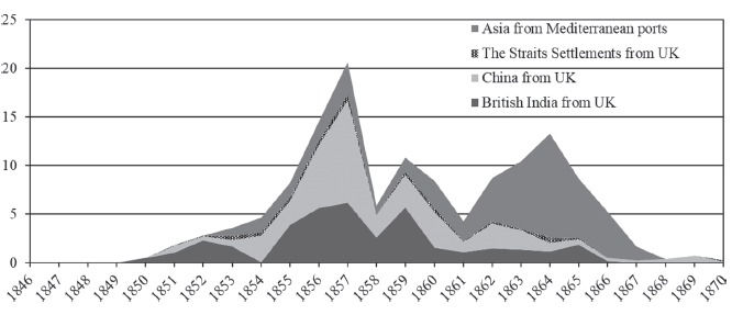
This section establishes a statistical overview of Asia’s silver absorption. Figure 1 shows the pattern of the silver influx in Asian countries from the United Kingdom and Mediterranean ports over 1846–1870. The figure documents that the silver influx into Asia gradually increased from 1850 until 1854, soared after 1855 and peaked at around 20 million pounds in 1857. Subsequently, a large amount of silver continued to flow into Asia until 1867. Concerning the origin of the silver influx, while the United Kingdom was the most significant supplier during the 1850s, Mediterranean ports began to supply Asia with massive silver after 1860.Footnote ¹ As the background of this change, most of the French silver collected in Paris was sent to Asia via London during the 1850s, as silver became scarcer in northern France, and the center of French silver exports moved from Paris to Marseille to reduce the transportation cost in the early 1860s (Flandreau Reference Flandreau2004, pp. 145–46). In addition, we find that India and China received the most silver influx from the United Kingdom. Thus, Asian countries, particularly India and China, imported massive quantities of silver from Europe between 1850 and 1867.Footnote ²

Figure 1

SILVER INFLUX IN ASIAN COUNTRIES FROM EUROPE, 1846–1870 (MILLION POUNDS STERLING)

Notes: “China from UK” and “Asia from Mediterranean ports” are export values. Others are import values. Value in Rupee were converted into Pound sterling by the exchange rates (Denzel Reference Denzel2010, pp. 500–1).

Sources: “Asia from Mediterranean” from The Economist (14 Mar. 1868, p. 49); “British India” from Bengal Commercial (1846–47); Bengal Trade (1848–70); Bombay Commercial (1846–47); Bombay Trade (1848–70); Madras Trade (1846–70); “The Straits Settlements” from Kobayashi (Reference Kobayashi2019); “China,” 1846–50 from Board of Trade (1859, p. 30); China 1851–58 was computed by deducting India’s and the Straits Settlements’ silver imports from the United Kingdom (after converting from import value (CIF) to export value (FOB) by deflating at 7 percent) from the total value of the U.K.’s silver exports to Asia (The Economist 14 Mar. 1868, p. 49); China 1859–67 from Ibid.; China 1868–70 from BPP (1871, p. 8). See Reference KobayashiKobayashi (2022).

STRUCTURE OF TRIANGULAR SETTLEMENT SYSTEM

As the background of Asia’s silver absorption, this section examines the structure of international settlements. It highlights the basic patterns of the trade balance among the United Kingdom, India, and China and demonstrates the importance of the triangular settlement system among them.Footnote ³

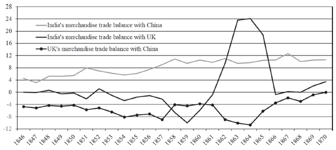
Figure 2 shows the merchandise trade balances of the United Kingdom with China and of India with the United Kingdom and China. First, the U.K.’s trade balance with China records a constant deficit. The U.K.’s deficit steadily increased until 1857, and after the peak in 1864, it decreased until 1867. We find that the development goes along with the pattern of silver influx shown in Figure 1. That is, silver was likely to move from the United Kingdom to China for the settlements. Meanwhile, Figure 2 documents that India’s trade balance with the United Kingdom was generally deficit, except for the huge surplus over 1862–65 caused by the cotton export boom in Bombay. In addition, India was obliged to remit to the United Kingdom around 7–10 million pounds annually owing to the Home Charges imposed on the English East India Company (EIC) until 1858 and on the Indian Office afterward (Chaudhuri Reference Chaudhuri, Kumar and Desai1983, pp. 870–73). Therefore, the situation of payment balance between India and the United Kingdom seems not to account for the silver influx in settlements, at a glance. However, the payment balance’s situation between them does not simply determine the pattern of settlements. Multilateral settlements were operating among the three countries.

Figure 2

TRADE BALANCE IN MERCHANDISE AMONG THE UNITED KINGDOM, INDIA, AND CHINA, 1846–1870 (MILLION POUNDS STERLING)

Notes: India’s trade balances represent aggregated values of three presidencies’ trade statistics (Bengal, Bombay, and Madras). Value in Rupee were converted into Pound sterling using the exchange rates (Denzel Reference Denzel2010, pp. 500–1).

Sources: Bengal Commercial (1846–47); Bengal Trade (1848–70); Bombay Commercial (1846– 47); Bombay Trade (1848–70); Madras Trade (1846–70); BPP (1859, pp. 8–9); BPP (1871, p. 5). See Reference KobayashiKobayashi (2022).

From the 1820s, the triangular trade grew among the United Kingdom, India, and China (Morse Reference Morse1910, p. 83; Tan Reference Tan1974). Under British colonial rule, India began exporting a large amount of opium to China, which brought up India’s constant trade surplus against China, as shown in Figure 2. Moreover, parts of the proceeds of opium exports were turned into Chinese tea and silk exports for the British market. During the same period, the United Kingdom rapidly increased exports of manufactured goods to India. Thus, the merchandise trade balances were partly offset among India’s surplus with China, China’s surplus with the United Kingdom, and the U.K.’s surplus with India, and the pattern lasted until the 1860s, as Figure 2 displays. Behind the growth of triangular trade, the multilateral settlements were functioning based on the circulation of bills of exchange among the three countries. That is, in China, some proceeds of Indian opium imports were converted into bills either for Indian cities or London, and finally used for remittance not only from China to India but also from India to the United Kingdom (Greenberg Reference Greenberg1951, pp. 156–57; Chaudhuri Reference Chaudhuri, Kumar and Desai1983, pp. 871–73). Thus, the development of remittance relying on exchange operations established the triangular settlement system.

Before looking into the specific mode of remittance, we point out that the primary financial organizations for exchange operations shifted from the EIC to private banks in Asia after 1850. Even after the cease of trade activity in 1833, the EIC had to transfer the revenue from India to the United Kingdom for the payment of dividends and Home Charges. Thus, the company maintained the remittance system by dealing with bills of exchange. Meanwhile, private merchant bankers also sold bills in the exchange market (BPP 1847/48, p. 116), and the “Eastern exchange banks” commenced exchange operations in Asian cities from the 1830s (Muirhead Reference Muirhead1996, p. 6).Footnote ⁴ Nevertheless, the EIC persistently objected to the Royal Charter grants offered to the exchange banks, which could have helped the banks raise enormous funds and expand their business. Consequently, the EIC maintained the dominant position in Asia’s exchange market until the late 1840s (Ibid., pp. 8–11). After 1850, however, the Eastern exchange banks began to acquire the Royal Charters and expanded their businesses to Asian metropolises (Suzuki Reference Suzuki, Nishimura, Suzuki and Michie2012, pp. 89–93). They consolidated the financial linkages between London and Asian cities via an extensive branch network and began to initiate the growth of Asia’s exchange market (Kitabayashi Reference Kitabayashi, Nishimura and Sugawara2020).

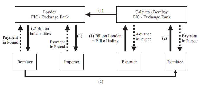
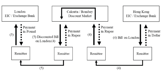
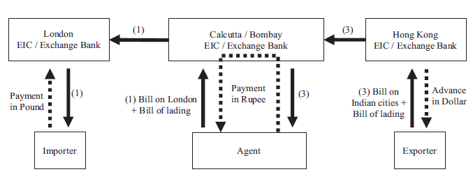
We look into the specific mode of remittance among the United Kingdom, India, and China referring to the descriptive sources and Figures 3–6. The figures exemplify the general patterns of remittance among the financial centers, namely London, Hong Kong, Calcutta, and Bombay. In the figures, the remitter sends a bill of exchange to remit, and the remittee is a recipient of the remittance. First, concerning the remittance between India and the United Kingdom (BPP 1831/32, pp. 106–19; BPP 1847/48, pp. 107–9; Crawfurd Reference Crawfurd and Kirti1837, pp. 288–90; Suzuki Reference Suzuki, Nishimura, Suzuki and Michie2012, pp. 87–88), the EIC and Exchange banks played a key role by issuing bills of exchange. In Indian cities, private merchants who exported goods to the United Kingdom drew bills on London and sold them to the EIC or banks to obtain advance payments in rupees (the arrows (1) in Figure 3). The EIC and banks accepted these bills from exporters with the attached bills of lading that guaranteed ownership of exported merchandise. Those bills were carried to London, and importers of Indian goods accepted the bills from the EIC’s or banks’ London offices by paying in pounds sterling. Then, importers collected the imports from a warehouse by submitting the bills of lading. Meanwhile, the London office sold the bills on Indian cities, and Britain’s remitters purchased and sent them to India (the arrows (2) in Figure 3). In India, the remittee who received the bill sold it to the EIC or banks in rupees. Through a series of exchange operations, the remittance was carried out without sending bullion.

Figure 3

REMITTANCE SYSTEM BETWEEN INDIAN CITIES AND LONDON

Sources: Author’s illustration. See details in the text.

Figure 4

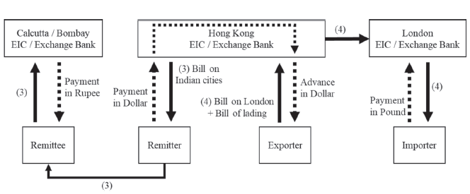
REMITTANCE SYSTEM FROM INDIAN CITIES TO LONDON VIA HONG KONG

Sources: Author’s illustration. See details in the text.

Figure 5

REMITTANCE SYSTEM FROM HONG KONG TO INDIAN CITIES VIA BILL ON LONDON

Sources: Author’s illustration. See details in the text.

Figure 6

REMITTANCE SYSTEM FROM LONDON TO HONG KONG VIA INDIAN CITIES

Sources: Author’s illustration. See details in the text.

Likewise, concerning the remittance between the United Kingdom and China, a bill of exchange was used as the primary mean (Crawfurd Reference Crawfurd and Kirti1837, pp. 288–89). The merchants in China, who dealt with consignments from the United Kingdom, sent Chinese goods to the United Kingdom. Simultaneously, they drew bills on London with bills of lading on exports and sold them in the exchange market to obtain advance payments in the dollar. These bills were purchased by the EIC and banks, which was the similar course of dealings with the arrows (1) in Figure 3. Furthermore, regarding the remittance between China and India, merchants who had to remit to India for the return of opium imports purchased the bills on Indian cities from the EIC and banks and sent them to the Indian remittee (BPP 1830b, pp. 353–54). The remittee brought bills in the EIC and banks to obtain payments in rupee. This was similar to the pattern of remittance with the arrows (2) in Figure 3.

Besides the direct remittance, the indirect remittance via the third country operated based on the growing triangular trade (BPP 1830b, pp. 12, 394–95, 418; BPP 1831/32, pp. 111–12). First, the remittance from India to the United Kingdom via China was carried out based on India’s trade surplus with China, as Figure 4 exemplifies. In Hong Kong, the EIC and banks sold bills on Indian cities to the merchants who had to remit to India, and received payments in the dollar (arrows (3) in Figure 4). Using the proceeds in the dollar, the EIC and banks discounted bills on London from exporters and sent the bills to London, and gave them to acceptors in return for payments in pound sterling (arrows (4) in Figure 4). We assume the Agency houses occasionally acted as both remitters and exporters in Hong Kong (Greenberg Reference Greenberg1951, pp. 156–58).

Likewise, the remittance from China to India was practiced using not only bills on Indian cities but also bills on London, as Figure 5 exemplifies (BPP 1830b, p. 370; Morse Reference Morse1910, pp. 84, 202). In Hong Kong, remitters purchased bills on London from the EIC and banks and sent them to remittees in Indian cities (arrows (4) in Figure 5). The remittee sold the bills on London in discount markets in Indian cities to receive payments in rupee. The bills sold there were purchased again and finally remitted to London (arrows (5) in Figure 5). In fact, the exchange rates of “China bills,” which were bills on London issued in China and sent to India, were quoted in Indian cities (Bombay Times January and February 1845). Additionally, another bill was provided through American trade. After the 1830s, American merchants purchased the bills on London from U.S. exports of raw cotton to Europe and sent them to China for payment of tea and silk imports. Those bills were bought by merchants who imported opium and sent it to India. Finally, they were sold as a means of remittance to the United Kingdom. Thus, the bill on London purchased in China was utilized for the remittance from China to India.

For the payment from the United Kingdom to China, the indirect remittance via India was feasible, as Figure 6 exemplifies. In this way, the agents in Indian cities played a key role by connecting Hong Kong’s exporter and London’s importer (Greenberg Reference Greenberg1951, pp. 157–58). First, in Hong Kong, exporters drew bills on Indian cities on exports of Chinese goods to the United Kingdom and sold them to the EIC and banks to gain advance payments in the dollar (arrows (3) in Figure 6). The bills were sent to Indian cities and accepted with the bills of lading by agents. Simultaneously, the agents drew bills on London with bills of lading and sold them to the EIC or banks (arrows (1) in Figure 6). Through this operation, the agents’ payment for the bills in Indian cities was offset. Ultimately, the bill was sent to London and accepted by importers of Chinese goods in exchange for payment in pound sterling.

The incentive for the indirect remittance was favorable exchange rates. Actually, for the direct remittance, the exchange rates tended to be unfavorable for the remitters and exporters in Asia due to the situation of payment balance. For instance, in Hong Kong, when exporters who shipped Chinese goods to the United Kingdom sold bills on London to gain advance payments, the exchange rates of pound sterling per dollar were inclined to be a disadvantage for them because of China’s constant trade surplus. Then, it could be favorable for them to sell bills on Indian cities, as Figure 6 exemplifies. For the remittance from India to the United Kingdom and from China to India too, the exchange rates of the deficit country’s currency against the surplus country’s currency tended to be unfavorable owing to the trade balance situation. Meanwhile, the remittance via the third country was practiced by combining the bills priced at favorable exchange rates, so the indirect mean tended to be beneficial for remitters.

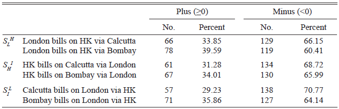
To establish the advantage of indirect remittance, we estimated the spread of indirect exchange rates against direct rates (detailed in Online Appendix I). Table 1 reports the number of observations when the spreads are situated plus or minus, together with the percentage against the total. For remittances from London to Hong Kong (see the S ^H rows in Table 1), if the spread is negative—that is, the indirect exchange rate’s pound against the dollar is stronger than that of the direct rate—it could be beneficial for remitters to practice indirect remittance via Indian cities. The positions of spreads in other series are interpreted in the same manner. The table documents that no less than 60 percent of the indirect rate’s observations were lower than the direct rates. Therefore, indirect remittance was feasible as a favorable means between the three countries. In sum, to analyze the settlement mechanism working for Asia’s silver absorption, it is appropriate to pay attention to the triangular settlement system as well as the bilateral settlement.

Table 1

SPREAD OF INDIRECT EXCHANGE RATES AGAINST DIRECT EXCHANGE RATES, JAN. 1846–DEC. 1866

Notes: , , and indicate the spread of indirect exchange rates against direct rates among London (L), Hong Kong (H), and Indian cities (I). See detail in Online Appendix I.

Sources: Hong Kong, Overland Register; China Overland Trade Report; The China Mail; Bengal Hurkaru; The Economist; Bombay Times; Bombay Times Standard; Times of India.

APPLICATION OF BULLION POINTS METHOD

To determine the best means of remittance among the United Kingdom, India, and China, merchants did not merely consider the exchange rates but also bullion market prices. As one merchant of the time stated: “All exchange operations in bills have reference to the actual produce of the remittance in bullion in the country to which those remittances are sent” (BPP 1831/32, p. 107). Remitters calculated “the bullion rate” by adding various costs for bullion shipping to its value. If a bill of exchange was not procurable at a cheaper rate than the bullion rate, bullion was remitted (Ibid., p. 111). However, as Chaudhuri (Reference Chaudhuri, Kumar and Desai1983) declared that “the actual mechanism of foreign exchange was quite complicated and sensitive to arbitrage operations between the various trading centres” (p. 871), the triangular settlement mechanism has not yet been revealed. This section argues the validity of the bullion point method for the analysis of Asia’s settlement and devises the formula of bullion points for the triangular settlement mechanism.

As a general tool, the specie point method has been applied to the analysis of settlement mechanisms between metallic standard systems (Morgenstern Reference Morgenstern1959, pp. 169–83; Officer Reference Officer1996, pp. 49–51, 107–13). The method reconstructs the specie points based on mint parity between two countries, calculated from the legally fixed metallic content in currencies (mint price), and examines the settlement mechanism adjusting imbalance of payments between the countries. First, we need to verify whether the specie point method applies to pre-1870 Asia’s settlement mechanism.

In our analysis period, the United Kingdom had been formally adopting the gold standard since 1821. As for India, the Bengal, Madras, and Bombay Presidencies under the EIC rule were using various rupee systems, such as Sicca, Arcot, and Bombay rupees, before the introduction of EIC Rupee in 1835 (Ellstaetter Reference Ellstaetter1895, pp. 1–2). The EIC rupee started to be coined at the mints in the three Presidencies to unify the Indian currency systems. However, while the EIC rupee came to prevail as the unit of account, the circulation of various old rupee coins persisted in the Presidencies and the Native States, and the gold currency also continued to be legally used until 1852 (Ibid., pp. 85–86; Tooke Reference Tooke and Kirti1857, pp. 178–79). Thus, we cannot simply regard the introduction of the uniform rupee system as the beginning of India’s silver standard. Regarding China’s currency, while the Qing government controlled the issue of copper coins, which were used for local retail trade, the private sector provided silver ingots sycee and silver dollars for tax payments and inter-provincial and foreign trade (Lin 2006, pp. 2–7). Particularly, since the late eighteenth century, Spanish dollars had prevailed as a medium of exchange for commerce in China, despite the fact that their supply was out of the state’s control (Ibid., pp. 44–48). The Chinese unit of weight and currency, tael, was used to value sycee, and its exchange rate with dollar was set based on the metallic contents of sycee and dollar coins, for example, 71.7 taels per 100 dollars in Canton. However, the exchange rates varied by cities and regions and fluctuated due to the premium attached to sycee and dollars in the local money market (King Reference King1965, p. 88). Regarding Hong Kong’s currency, while sycee and dollars were current at the market rate since the foundation of the British colony in 1842, the colonial government sought to set pound sterling as a legal tender to bring the currency into the British monetary system. However, the attempt fell through because the British gold coin was unfamiliar to Chinese merchants, and eventually, the Mexican silver dollar was legalized in Hong Kong in 1854 (Ibid., pp. 182–84). Subsequently, the local mint started coining the Hong Kong dollar modeled after the Mexican dollar in 1866, but Chinese locals avoided using the coins and melted them into bullion, causing the mint to close down two years later (Ibid., p. 185). Thus, during our analysis period, Hong Kong’s currency was nearly the same as the Chinese system and essentially part of the currency area of China.

During our analysis period, the United Kingdom and China were not sharing a common metallic standard. Moreover, because the Chinese government did not mint the silver currencies on its own account, the legal mint price was not established there. Regarding the dollar unit used for foreign trade, the exchange rate with tael virtually fluctuated according to the premium on silver in the local market. Hence, it is unreasonable to assume mint parity between them. Likewise, the remittance between the U.K. gold standard and India’s silver standard was not as simple as the specie point mechanism. London remitters could send not only silver but also gold because both metallic coins were circulating in India. Similarly, besides gold shipments, Indian remitters were able to send silver and convert it into pounds sterling in the London bullion market. Thus, we cannot ensure the validity of mint parity between them. As for the settlements between India and China, despite the similarity in the prevalence of silver circulation, it is uncertain whether the Indian rupee and sycee or dollar used in China held the constant mint parity. In sum, all these elements suggest that we should avoid adopting the specie point method.

Instead, the “bullion point” method is suitable for our analysis. The method elaborated in studies of bimetallism allows us to analyze the settlement mechanism between heterogeneous monetary systems (Flandreau Reference Flandreau2004, ch. 3; Nogues-Marco Reference Nogues-Marco2013). The key difference in bullion points from the specie points is that it relies on the “arbitrated par.” This par does not use legal mint prices but relies on bullion market prices. We define the silver arbitrated par in London to Hong Kong as (term p _s for the silver price, and exponents L and H for London and Hong Kong, respectively). Thus, we calculate the “silver bullion points” by adding or deducting arbitrage cost (terms and , HL means shipping from Hong Kong to London, and vice versa) to and from the arbitrated par, which regulates the variations of exchange rate , as expressed in Equation (1)

(1) $$(1 - c_s^{HL}){{p_s^L} \over {p_s^H}} \le X_L^H \le (1 + C_s^{LH}){{p_s^L} \over {p_s^H}}$$

Depending on the payment balance’s situation, this formula defines the adjustment mechanism in which the equilibrium exchange rate settles somewhere within the silver bullion points (the left side is import points, and the right is export points in the inequality). If London’s deficit against Hong Kong has to be cleared, bills on Hong Kong become scarce, and the exchange rate rises toward the export point. Conversely, London’s surplus brings superabundant claims on Hong Kong, leading the exchange rate to fall toward the import point. If the exchange rates exceeded the export or import points, silver moves between them instead of bills of exchange, and it adjusts the demand for bills and restores the equilibrium exchange rate.

Likewise, in Equation (1), the silver bullion points are based on two variables, and , so the adjustment takes place not only when the London silver price fluctuated but also when the Hong Kong one did. Moreover, the adjustment operates through reciprocal variations in both markets. When the silver price fluctuation in either market led to the violation of the exchange rate and silver moved between markets, in the remitter’s market, besides adjusting the demand for bills, the silver efflux is expected to induce an appreciation for silver. Meanwhile, the market that underwent silver influx faces its depreciation, leading to an equilibrium between the two markets (Flandreau Reference Flandreau2004, pp. 68–70). In other words, the strength of bullion points lies in highlighting the adjustment mechanism for both the exchange rate system and the international bullion market. This distinct feature, adjustment for the international bullion market, is essentially important for our analysis because we aim to capture how Asia’s settlement system operated for the silver absorption, which buffered the Gold Rushes’ shock on the international bullion market. Furthermore, because this method targets both the metallic standard establishing mint price and the currency system, which consisted of various bullion and currency, it is also suitable for the analysis of settlements between diverse currency systems. Hence, this method enables us to analyze the settlement mechanism among the United Kingdom, India, and China in the mid-nineteenth century.Footnote ⁵

We obtain the same equations for silver bullion points (hereafter silver points) in Indian cities (exponent I) with London (Equation 2), and in Hong Kong with Indian cities (Equation 3). The original method formulates the “gold points” as well as silver points and derives “bullion points” from the silver and gold points (Ibid., pp. 59–61). However, if we would elaborate on both silver and gold points, the complete version of bullion points for the triangular settlements includes many terms and becomes too complicated to understand the essentials. In fact, as shown later, the analysis of silver points adequately demonstrates the settlement mechanism for Asia’s silver absorption. Hence, we focus on the silver points afterward.

(2) $$(1 - c_s^{LI}){{p_s^I} \over {p_s^L}} \le X_I^L \le (1 + c_s^{IL}){{p_s^I} \over {p_s^L}}$$

(3) $$(1 - c_s^{IH}){{p_s^H} \over {p_s^I}} \le X_H^I \le (1 + c_s^{HI}){{p_s^H} \over {p_s^I}}$$

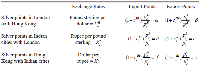
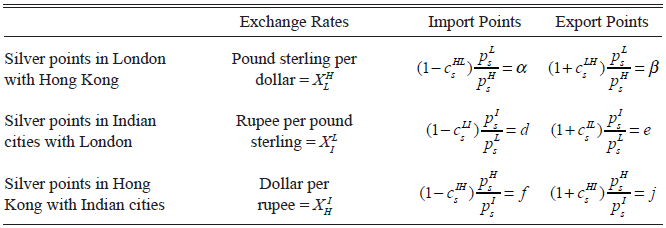
The formulas define the settlement mechanism between the two places, namely, “the bilateral silver points.” However, it is indispensable for the analysis of Asia’s silver absorption to investigate the triangular settlement mechanisms. For this purpose, we adapt the formulas for bilateral silver points to an applicable form for the triangular settlements. From Equations (1)–(3), after simplifying the terms of silver points according to Table 2, we obtain Equation (4) defining the triangular silver point mechanism in London with Hong Kong. Online Appendix II summarizes how to develop the formulas.

(4) $$Max\{ \alpha (f/X_H^I);\,\alpha (d/X_I^L);\alpha \} \le X_L^H \le Min\{ \beta ;\,\beta (j/X_H^I);\,\beta (e/X_I^L)\} $$

Table 2

FORMULA TERMS FOR SILVER POINTS IN LONDON, INDIAN CITIES, AND HONG KONG

Sources: Author’s elaboration. See details in the text.

Equation (4) writes that the silver points are composed of either bilateral points (α and β, see Table 2) or those with the parameters ; and ; . We call the latter “triangular silver points.” They are affected by and ; namely, the relationship between the bilateral import and export points (f and j respectively, see Table 2) and the exchange rates in Hong Kong with Indian cities, and by and , or the relationship between bilateral import and export points (d and e respectively, see Table 2) and the exchange rate in Indian cities with London. In other words, as long as the equilibrium in the triangular settlement system holds, that is, all exchange rates in London and Asian cities settle within the band of bilateral silver points , the bilateral points constitute the effective import and export bounds. However, when the exchange rates violate the bounds in other settlement systems < 1), the triangular silver points compose the effective import or export bounds in London with Hong Kong, and the band becomes narrower than the bilateral silver points. This settlement mechanism indicates that even if silver shipment from London to Hong Kong was an unfavorable mean of remittance compared to bills of exchange, remitters could send silver as long as the bullion arbitrage either from Hong Kong to Indian cities or from Indian cities to London was profitable enough to compensate the loss caused by the silver remittance. Then, if the silver was actually shipped in response to the triangular export points, the demand for bills of exchange decreases and the exchange rates are regulated by the narrower band. The fifth section will elaborate on this mechanism by exemplifying the arbitrage operations.

We can interpret that the triangular silver point mechanism works not only to adjust imbalances in exchange and bullion markets between the two places but also to maintain monetary equilibrium among the three places. Particularly, as a remarkable function, the triangular silver points stabilize exchange rates by generating a narrower band than that of the bilateral points. In other words, when the triangular points are effective because the arbitrage cost defined by the narrower band becomes less than the bilateral points, the cost efficiency for silver trade improves. Thus, the triangular settlement mechanism theoretically equilibrates imbalances more efficiently than the bilateral settlement does. Besides Equation (4), we obtain the same equations regarding the triangular settlement mechanisms in Indian cities with London and in Hong Kong with Indian cities (see Online Appendix II). Thus, to reconstruct triangular silver points, we apply the formulas to the new financial dataset.

RECONSTRUCTION OF BILATERAL AND TRIANGULAR SILVER POINTS

The first step toward the reconstruction of bilateral and triangular silver points requires establishing the arbitrated pars of silver between the two markets. To this end, we collected a new series of monthly bullion prices in Hong Kong, Calcutta, and Bombay from 1846 to 1870 (see Online Appendix III). The commercial newspapers of Asian cities published “bullion prices,” namely, the quotations of ingots and foreign currencies. Thus, we derived the unit price (per troy ounce) of silver from these publications, in line with the standard metallic contents (see Online Appendix III).

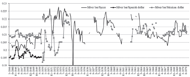
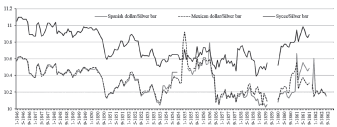
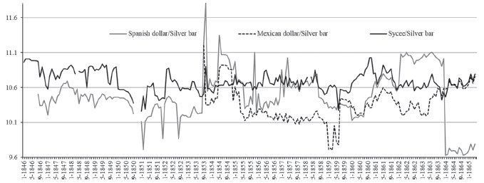
Before computing the arbitrated pars, we should scrutinize the nature of silver prices in Asia. We derived the silver prices in Asian cities from the quotations of a particular form of silver, such as Chinese silver ingot sycee, and Spanish and Mexican dollars. They were quoted as premium in Hong Kong and as a quotation in rupee in Calcutta and Bombay. They represent the prices of particular silvers in Asian cities, and their ranges and variations definitely differed from each other. Consequently, while the single series of silver prices (silver bar) in London are available, there are a few types of silver prices in Asian cities, namely, sycee, Spanish dollar, and Mexican dollar. Figures 7–9 show the different series of silver arbitrated pars in London with Hong Kong and in Indian cities with London over 1846–1870. All the series were derived from the combination of the prices of different sorts of silver. These figures clarify that the arbitrated pars of silver between London and Asian cities considerably varied by each kind of silver.

Figure 7

SILVER ARBITRATED PARS IN LONDON WITH HONG KONG, JAN. 1846–DEC. 1870 (POUND PER DOLLAR)

Notes: The series were computed by dividing London’s silver prices by Hong Kong’s silver prices, as arbitrated pars for export points (see “Time lag” in Online Appendix III).

Sources: Hong Kong, Overland Register; China Overland Trade Report; The China Mail; Spalding (Reference Spalding1924, p. 330); Schneider, Schwarzer, and Zellfelder (Reference Schneider, Schwarzer and Zellfelder1991, pp. 265–67). See Reference KobayashiKobayashi (2022).

Figure 8

SILVER ARBITRATED PARS IN CALCUTTA WITH LONDON, JAN. 1846–DEC. 1862 (RUPEE PER POUND)

Notes: The series were computed by dividing Calcutta’s silver prices by London’s silver prices, as arbitrated pars for export points (see “Time lag” in Online Appendix III).

Sources: Bengal Hurkaru; Spalding (Reference Spalding1924, p. 330); Schneider, Schwarzer, and Zellfelder (Reference Schneider, Schwarzer and Zellfelder1991, pp. 265–67). See Reference KobayashiKobayashi (2022).

Figure 9

SILVER ARBITRATED PARS IN BOMBAY WITH LONDON, JAN. 1846–MAY 1865 (RUPEE PER POUND)

Notes: The series were computed by dividing Bombay’s silver prices by London’s silver prices, as arbitrated pars for export points (see “Time lag” in Online Appendix III).

Sources: Bombay Times; Bombay Times Standard; Times of India; Spalding (Reference Spalding1924, p. 330); Schneider, Schwarzer, and Zellfelder (Reference Schneider, Schwarzer and Zellfelder1991, pp. 265–67). See Reference KobayashiKobayashi (2022).

The price gaps between particular silvers in Asian cities were caused by the different demands for each silver. It was a particularly outstanding feature of China’s monetary system. From the 1820s, China faced a short supply of Spanish dollars in the aftermath of the Latin American countries’ independence. Meanwhile, Chinese merchants avoided accepting the new Mexican dollar coin that was debased after the Mexican Republic’s independence (Irigoin Reference Irigoin2009a, pp. 556–57). Consequently, Spanish dollars bore a high premium in China, and some dollars were circulating chopped or stamped on the surface as a mark of reliability (BPP 1857/58, p. 50; Williams and Morrison 1856, p. 290). Consequently, to make an arbitrage profit from the high premium on the Spanish dollar, merchants imported dollars in China and exported sycee to the mints in India and London (Ibid., pp. 355–56; Irigoin Reference Irigoin2013, pp. 20–23). Finally, the silver outflows from China ceased in 1856 when the Mexican dollar began to be imported and widely current in Chinese cities (Williams and Morrison 1856, p. 162). Likewise, the bullion prices in Indian cities were affected by the silver arbitrage in China. Because sycee imported from China yielded arbitrage profits by being brought into the mints, its price was quoted higher than dollars in Indian cities (see Figures 8 and 9). Also, according to the bullion market quotations published in the 1840s, the Spanish dollar was quoted separately from the silver bar in London (BPP 1847/48, pp. 211–17).

Thus, we should distinguish the prices of different silvers in London and Asian cities. For instance, in estimating the arbitrated pars in London with Hong Kong, we cannot combine the prices of the silver bar in London and the Spanish dollar in Hong Kong. They were priced separately as a particular sort of silver in each market. Even if the remitter sent the silver bar from London to Hong Kong, it was not priced according to the premium on the Spanish dollar in the recipient’s market. Hence, to calculate the silver arbitrated pars, we should combine silver prices of the identical or similar bullion. Between Hong Kong and Indian cities, we can make a pair of the same ingot (sycee) or coin (Spanish or Mexican dollar) to compute the effective arbitrated pars. However, concerning the arbitrated pars between London and Asian cities, we need to find which silver’s price in Asian cities corresponds with the silver bar’s price in London.

A book written by Ernest Seyd, a bullion broker, suggests that tael, as a Chinese unit of account, became the standard for pricing the silver bars in the Chinese market (Seyd Reference Seyd1868, pp. 418–19). According to this information, when silver bars were imported into Hong Kong, they were priced in tael, reflecting the premium on silver in the local market. For estimating proceeds, this unit was converted into dollars using the exchange rate of 0.717 taels per dollar, which was derived from the metallic contents of sycee and dollar coin. Because tael was a unit of measurement to value sycee, it is likely that its premium quoted in the local market was equivalent to the premium for pricing the silver bars imported into Hong Kong. Thus, we can employ the quotations of sycee in Hong Kong as a corresponding price with silver bar’s price in London. As for the silver prices in Indian cities, while the rupee quotations of the Spanish dollar, Mexican dollar, and sycee are available, we could not obtain the silver bar’s price. The previously-cited source (Ibid., pp. 409–14) explains that the silver bars imported from the United Kingdom in Indian cities were sold in the local bazaars, and after being priced at the market quotations, the metals were brought into the mint and sold at the mint price. This course of dealings was similar to the transactions of sycee after being imported from China into India (Williams and Morrison 1856, pp. 355–56). Meanwhile, as discussed earlier, the dollar coins were sent to China to make arbitrage profit from the extraordinary premium on the Spanish dollar. The quotations of dollars in Indian cities exactly represent the prices of “silver dollars” and do not match with the price of the silver bar. Therefore, we judged that the quotations of sycee better fit the corresponding price for British silver bar imported into Indian cities.

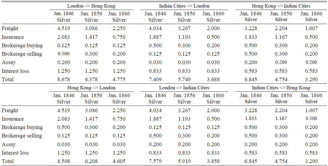
We computed the arbitrated pars of silver between London and Asian cities using the quotations of silver bar and sycee and the arbitrated pars between Hong Kong and Indian cities using the quotations of sycee. Based on these pars, we reconstructed the silver points. The arbitrage costs between the cities were summarized in Online Appendix III and Table 3. The import and export points were computed by adding and deducting these costs to and from the arbitrated pars. In applying the costs to the monthly series of arbitrated pars, given the gradual decline of arbitrage costs over time, we interpolated between Jan. 1846 and Jan. 1856, between Jan. 1856 and Jan.1866, and extrapolated from Jan. 1866 until Dec. 1870. We note that the costs were estimated based on the sources sparsely recorded during the 1830s–60s, so the reconstructed silver points include the measurement errors. However, we attempted to collect the information as thoroughly as possible and verified its validity (see Online Appendix III). Accordingly, our reconstructed silver points do not largely deviate from the true rates that remitters were practically relying on.

Table 3

ESTIMATED ARBITRAGE COSTS AMONG LONDON, HONG KONG, AND INDIAN CITIES (PERCENT)

Sources: See the text and Online Appendix III.

Regarding the interpretation of the silver point mechanism, our focus is the position of the exchange rates in relation to the silver points. Basically, the exchange rate varies depending on the payment balance’s situation. If the exchange rate approaches the bounds of silver points, silver is likely to be remitted. Conversely, the further away the rate is from the bounds, the less likely silver trade is. Then, the bill of exchange becomes a favorable instrument for remittance. Of course, as noted earlier, because the series are estimates and there might be speculative bullion shipments, silver trade could occur even before the exchange rate hits the bounds (Flandreau Reference Flandreau2004, p. 61). In sum, the position of the exchange rates against silver points indicates the probability of silver arbitrage between the two places.

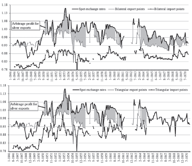
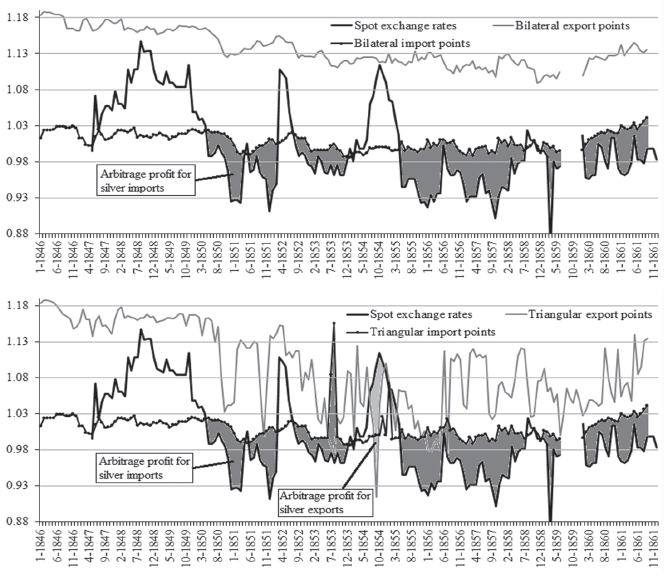
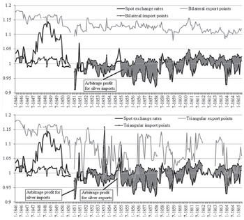
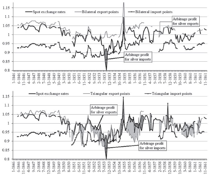
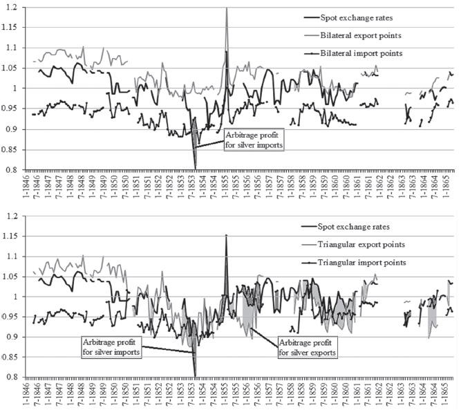
Specifically, we see the reconstructed silver points from Figures 10–14. In the figures, the gray-colored parts represent the range of the exchange rates’ violation to the bounds or the profit margin for arbitrage. At this point, we attempt to see the tendencies of arbitrage profits’ emergence and the difference between the bilateral and triangular settlements. The next section will elaborate on the arbitrage profits. First, Figure 10 shows that the exchange rates started exceeding the export bounds of both bilateral and triangular points in London with Hong Kong after 1850, and the substantial profit lasted until 1870. Likewise, in Figures 11 and 12, the exchange rates began violating the import bounds of both bilateral and triangular points in Indian cities with London after 1850, and the tendency persisted until the early 1860s. Overall, silver exports from London to Hong Kong and silver imports from London in Calcutta and Bombay became more favorable than bills of exchange, so there were arbitrage profits for the silver influx from the United Kingdom into China and India. Meanwhile, Figures 13 and 14 show that while ranging close to the export bounds, the exchange rates moved within the bands of bilateral points in Hong Kong with Calcutta and Bombay. However, as for the triangular points, the band became much narrower than the bilateral points, and the exchange rates frequently exceeded the export and import bounds. Thus, regarding settlements in Hong Kong with Indian cities, while the bilateral silver point mechanism seemed to maintain the equilibrium exchange rates, the imbalances arising in the triangular settlement system brought substantial arbitrage profits for the silver trade. The next section examines what these differences indicate for Asia’s silver absorption.

Figure 10

EXCHANGE RATES AND BILATERAL AND TRIANGULAR SILVER POINTS IN LONDON WITH HONG KONG, JAN. 1846–DEC. 1870

Notes: Variables were normalized by the arithmetic mean of the spot exchange rates in the entire period.

Sources: Hong Kong, Overland Register; China Overland Trade Report; The China Mail; Spalding (Reference Spalding1924, p. 330); Schneider, Schwarzer, and Zellfelder (Reference Schneider, Schwarzer and Zellfelder1991, pp. 265–67); Table 3. See Reference KobayashiKobayashi (2022).

Figure 11

EXCHANGE RATES AND BILATERAL AND TRIANGULAR SILVER POINTS IN CALCUTTA WITH LONDON, JAN. 1846–DEC. 1861

Notes: Variables were normalized by the arithmetic mean of the spot exchange rates in the entire period.

Sources: Bombay Times; Bombay Times Standard; Times of India; Spalding (Reference Spalding1924, p. 330); Schneider, Schwarzer, and Zellfelder (Reference Schneider, Schwarzer and Zellfelder1991, pp. 265–67); Table 3. See Reference KobayashiKobayashi (2022).

Figure 12

EXCHANGE RATES AND BILATERAL AND TRIANGULAR SILVER POINTS IN BOMBAY WITH LONDON, JAN. 1846–APRIL 1865

Notes: Variables were normalized by the arithmetic mean of the spot exchange rates in the entire period.

Sources: Bengal Hurkaru; Spalding (Reference Spalding1924, p. 330); Schneider, Schwarzer, and Zellfelder (Reference Schneider, Schwarzer and Zellfelder1991, pp. 265–67); Table 3. See Reference KobayashiKobayashi (2022).

Figure 13

EXCHANGE RATES AND BILATERAL AND TRIANGULAR SILVER POINTS IN HONG KONG WITH CALCUTTA, JAN. 1846–DEC. 1861

Notes: Variables were normalized by the arithmetic mean of the spot exchange rates in the entire period.

Sources: Hong Kong, Overland Register; China Overland Trade Report; The China Mail; Bengal Hurkaru; Table 3. See Reference KobayashiKobayashi (2022).

Figure 14

EXCHANGE RATES AND BILATERAL AND TRIANGULAR SILVER POINTS IN HONG KONG WITH BOMBAY, JAN. 1846–APRIL 1865

Notes: Variables were normalized by the arithmetic mean of the spot exchange rates in the entire period.

Sources: Hong Kong, Overland Register; China Overland Trade Report; The China Mail; Bombay Times; Bombay Times Standard; Times of India; Table 3. See Reference KobayashiKobayashi (2022).

TRIANGULAR SETTLEMENT MECHANISM FOR ASIA’S SILVER ABSORPTION

This section examines how the bilateral and triangular settlement mechanisms affected the silver trade among the United Kingdom, India, and China. Theoretically, the synchronization between the emergence of arbitrage profit and the increase in bullion trade is one indicator that the bullion point mechanism was functioning properly. To capture this relationship, we extract the annual arbitrage profit rates from the reconstructed silver points and compare them with the annual silver trade. To estimate the annual profit rate of silver arbitrage, we set the following equations.

(5) $$SE{P_y} = \sum\limits_k^{K + 11} {(EX{R_{y,k}} - EX{P_{y,k}}|\,EX{R_{y,k}} > EX{P_{y,k}})} $$

(6) $$SI{P_y} = \sum\limits_k^{K + 11} {(IM{P_{y,k}} - EX{R_{y,k}}|\,IM{P_{y,k}} > EX{R_{y,k}})} $$

In both equations, y is the year and k is the starting month for the calculation. SEP stands for Silver Export Profits, SIP for Silver Import Profits, and EXR for (spot) Exchange Rate. EXP stands for Export Points and IMP for Import Points. Hence, SEP and SIP are the gross profit computed by deducting the costs from the earnings. To compare with the annual silver imports and exports, we calculated the annual sum of monthly profit margins in accordance with the official year of the Indian trade statistics, from May (k = 5) to April of the next year, except for that between London and Hong Kong, which was based on the calendar year (k = 1). As a prerequisite, we computed the profit margins only when the exchange rates exceeded the export or import bounds, as stated in both equations. The time horizon y starts from 1846 and ends in various years, according to the data availability (see Figures 10–14).

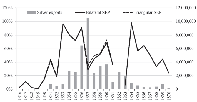
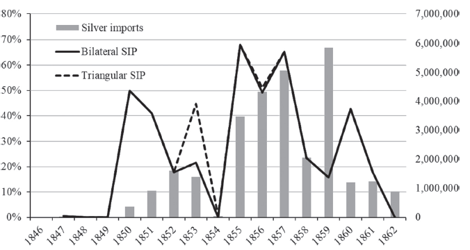
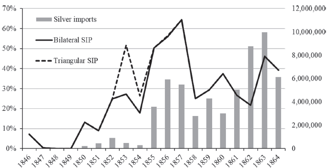
Figures 15–17 show the estimated arbitrage profit rates and volume of silver trade in London with Hong Kong and in Indian cities with London. As previously noted, these profit rates are estimates and not a determinant factor for the bullion trade. Even if we did not derive any profit in a certain year, there might be speculative bullion shipments, and we can suppose that because silver was traded responsively when arbitrage opportunities emerged, the exchange rates could stay within the silver points. However, it is certain that the emergence of large profit rates became the strong incentive for arbitrageurs to trade silver on a large scale. Another caveat is that the data on the silver trade includes not only bullion but also coins. It follows that we compare the arbitrage profits derived from the quotations of silver bar and sycee with the entire silver trade, including dollars.

Figure 15

ARBITRAGE PROFIT RATE AND SILVER EXPORTS IN LONDON (THE UNITED KINGDOM) WITH HONG KONG (CHINA), 1846–1870

Notes: Arbitrage profit rate per unit of silver export value (left axis) and silver exports from the United Kingdom to China in pound sterling (right axis).

Sources: See Figure 1 for silver exports and Figure 10 for arbitrage profit. See Reference KobayashiKobayashi (2022).

Figure 16

ARBITRAGE PROFIT RATE AND SILVER IMPORTS IN CALCUTTA WITH LONDON (THE UNITED KINGDOM), 1846–1862

Notes: Arbitrage profit rate per unit of silver import value (left axis) and silver imports in pound sterling (right axis). Silver imports are an aggregated value of imports from the United Kingdom, Aden, and Suez. Because India’s trade statistics recorded the trade with Aden and Suez, including transit trade with Europe, it is appropriate to aggregate them to capture the actual volume of silver trade.

Sources: Silver imports from Bengal Commercial (1846–47); Bengal Trade (1848–62). See Figure 11 for arbitrage profit. See Reference KobayashiKobayashi (2022).

Figure 17

ARBITRAGE PROFIT RATE AND SILVER IMPORTS IN BOMBAY WITH LONDON (THE UNITED KINGDOM), 1846–64

Notes: Arbitrage profit rate per unit of silver import value (left axis) and silver imports in pound sterling (right axis). Silver imports are aggregated value of imports from the United Kingdom, Aden, and Suez. See Figure 16.

Sources: Silver imports from Bombay Commercial (1846–47); Bombay Trade (1848–64). See Figure 11 for arbitrage profit. See Reference KobayashiKobayashi (2022).

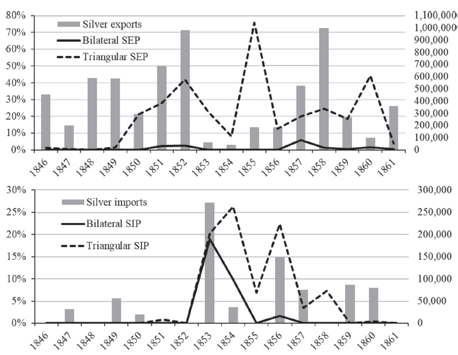
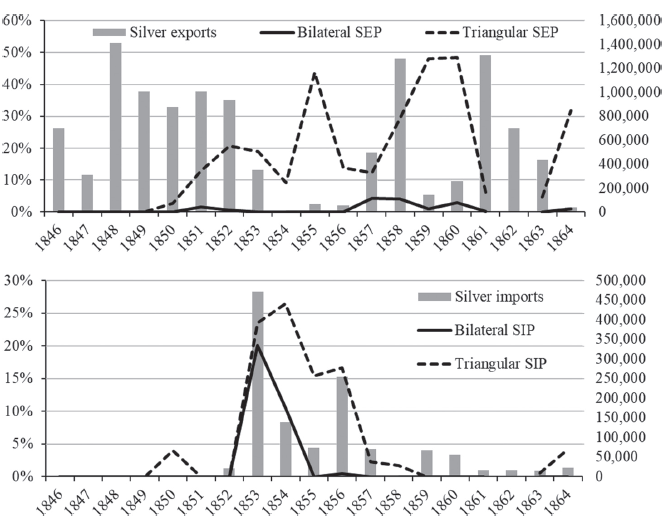
There is fragmentary information saying that the United Kingdom chiefly exported silver coins to China and silver bullions to India (Board of Trade 1859, p. 30). However, because the accurate trade data distinguishing the kinds of silver is not currently available, we proceed to the comparison with the assumption that the major part of silver trade among the three countries consisted of the silver bar or sycee. From Figures 15–17, we find that the arbitrage profits remarkably increased from 1850 onwards, and the silver trade started to increase concurrently. Regarding the difference between the bilateral and triangular arbitrage profits, except for 1853 in Figures 16 and 17, there is little gap between them. In other words, the silver influx from the United Kingdom in China and India was induced by the arbitrage profit arising from the bilateral settlement mechanism. Meanwhile, the triangular settlement system seems not to affect the silver influx.

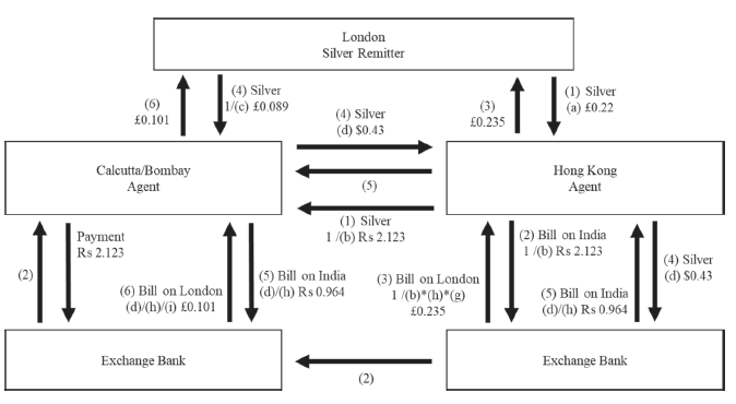
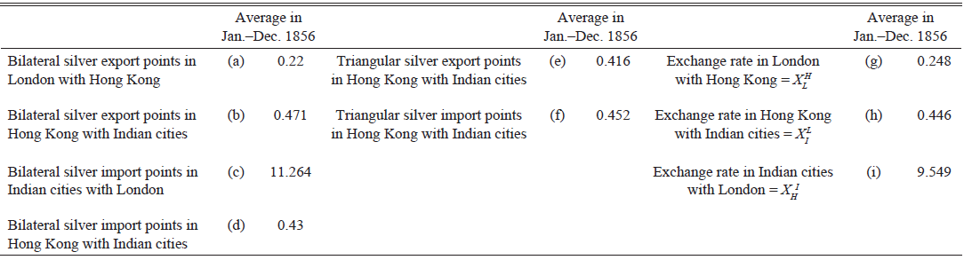
However, regarding the intra-Asian settlement, the difference between bilateral and triangular arbitrage profits evidently appeared. Figures 18 and 19 show the arbitrage profits and silver trade in Hong Kong with Calcutta and Bombay. Looking into SEP, while the bilateral SEP maintained the neutral value throughout the years, the triangular SEP began increasing after 1850. This gap was caused by what the increase of bilateral SEP in London with Hong Kong (see Figure 15) affecting the SEP in Hong Kong with Indian cities through the triangular settlement mechanism, as expressed in Equation (4) Moreover, regarding SIP, although both bilateral and triangular SIP rose in 1853, while the bilateral SIP diminished by 1855, the triangular SIP was sustained at relatively large rates until 1858. The persistence of the triangular SIP was brought about by the expanding SIP in Indian cities with London (see Figures 16 and 17) via the triangular settlement mechanism. Thus, the triangular settlement mechanism is likely to account for the pattern of silver trade between China and India after 1850, better than the bilateral settlement. In other words, the intra-Asian silver trade occurred as a part of the silver influx from the United Kingdom into Asia after 1850 based on the triangular settlement mechanism. We substantiate this mechanism by exemplifying specific arbitrages as follows. Figure 20 exemplifies the arbitrage operations using the average exchange rates and silver points in 1856, as Table 4 presents. We selected the example in 1856 because in that year, both the triangular SEP and SIP in Hong Kong with Indian cities rated the distinctly larger values than those of bilateral ones, and silver moved mutually between China and India, so the situation provides us with a useful case to understand the triangular arbitrage operations. In the course of operations, we establish the significant role of “Agent,” which fits the function of Agency house (Greenberg Reference Greenberg1951, pp. 157–58). The agents in Hong Kong and Indian cities are consignees to receive silver from London and send back the proceeds of selling silver in Asian markets. Simultaneously, because the precondition is the triangular settlements, the Hong Kong agent is obliged to remit to the agents in Indian cities, and vice versa (e.g., in Figure 6, as well as having a claim against London, the Indian agent owes bills on India drawn in Hong Kong). Therefore, for the intra-Asian remittance, the agents re-export silver imported from the United Kingdom in response to the arbitrage profit. Actually, part of the silver exported from the United Kingdom to India was again sent to China to pay for the increasing exports of Chinese products to Britain (Tooke Reference Tooke and Kirti1857, pp. 173–74). For the intra-Asian silver trade, we assume that these agents collaborate. Practically, when they choose the remittance means, or either bill or silver, they refer to the bilateral silver points for each dealing, but virtually speculate arbitrage profits derived from the triangular settlement system.

Figure 18

ARBITRAGE PROFIT RATE AND SILVER EXPORTS AND IMPORTS IN HONG KONG (CHINA) WITH CALCUTTA, 1846–1861

Notes: Arbitrage profit rate per unit of silver export and import value (left axis) and silver exports and imports in pound sterling (right axis). Silver exports and imports were derived from Calcutta’s silver imports and exports with China by converting the import values (CIF) into export values (FOB) at 7 percent deflation, and vice versa.

Sources: Silver exports and imports from Bengal Commercial (1846–47); Bengal Trade (1848– 61); see Figure 13 for arbitrage profits. See Reference KobayashiKobayashi (2022).

Figure 19

ARBITRAGE PROFIT RATE AND SILVER EXPORTS AND IMPORTS IN HONG KONG (CHINA) WITH BOMBAY, 1846–1864

Notes: Arbitrage profit rate per unit of silver export and import value (left axis) and silver exports and imports in pound sterling (right axis). Silver exports and imports were derived from Bombay’s silver imports and exports with China by converting the import values (CIF) into export values (FOB) at 7 percent deflation, and vice versa.

Sources: Silver exports and imports from Bombay Commercial (1846–47); Bombay Trade (1848–64); see Figure 14 for arbitrage profits. See Reference KobayashiKobayashi (2022).

Figure 20

DEMONSTRATION OF SILVER ARBITRAGE OPERATIONS IN THE TRIANGULAR SETTLEMENT SYSTEM (1856)

Sources: Author’s illustration.

Table 4

AVERAGE EXCHANGE RATES AND SILVER POINTS IN 1856

Sources: See Figures 10–14 and details in the text.

We begin to simulate that the London bullion dealer sends silver at the value of 1 dollar to Hong Kong, which costs 0.22 pounds sterling (see (a) in Table 4 and arrows (1) in Figure 20). The Hong Kong’s agent re-exports the silver to Indian cities before returning the proceeds to London. Although the silver shipment to India is an unfavorable mean of remittance in the bilateral settlement because the exchange rate (h) is priced lower than silver export points (b), the agent can send silver because the exchange rate is higher than the triangular silver export points (e), promising the arbitrage profit. Thus, Hong Kong’s agent remits the silver at the value of 2.123 rupees to Indian cities (arrows (1)) and draws the bill on India on the silver exports (arrows (2)). The bill on India is sold to Exchange bank in return for the bill on London converting 2.123 rupees into 0.235 pounds sterling, via the exchange rates (h) and (g). Finally, the bill on London (arrows (3)) was sent from Hong Kong to London as the proceeds of silver trade with a profit margin of 0.015 (0.235–0.22) pounds sterling. Meanwhile, the Indian cities’ agent receiving silver from London at the value of one rupee, costing 0.089 pounds sterling (1/(c) and arrows (4)), also re-exports the metal to Hong Kong. Regarding this case too, while the silver remittance is unfavorable due to the higher value of the exchange rates (h) compared to the bilateral import points (d), the speculation by the triangular import points (f), that is higher than the exchange rates, allows the agent to send silver to Hong Kong. The silver landed in Hong Kong and priced at 0.43 dollars (d) at minimum was sold to the Exchange bank in return for the bill on India 0.964 rupees (arrows (5)). Hong Kong’s agent sends the bill to India’s agent as the proceeds of the silver trade, and the bill was accepted by the bank in Indian cities in return for the bill on London priced at 0.101 pounds sterling, by converting 0.964 rupees via the exchange rate (i). Ultimately, the bill was sent to London as the turnover of silver trade with profit margin 0.012 (0.101–0.089) pounds sterling (arrows (6)).

From the demonstration, we find that the silver flow between China and India could yield arbitrage profits via the triangular settlement mechanism, despite the fact that the intra-Asian settlement in itself does not make any arbitrage profits. Specifically, the demonstration revealed that the key transaction yielding profit is the conversion of bills on India into bills on London in Hong Kong and Indian cities (exchange between arrows (2) and (3), and between (5) and (6)). Then, the indispensable condition was what the exchange rates of local currencies, dollar and rupee, against pound sterling are strong enough to exceed the bounds of bilateral silver points and make large arbitrage profits. The condition is expressed as “triangular silver points” in Equation (4), and it generates the narrower band regulating the exchange rates efficiently. This mechanism worked out in the demonstration. Focusing on the demand and supply on bills, we see that the intra-Asian silver trade would induce the rising demand on bills on London (arrows (3) and (6)) so that the imbalance of exchange and bullion markets, or the fall of the pound sterling and silver appreciation in Asian cities with London could be stabilized not only by the silver influx from the United Kingdom but also via intra-Asian silver trade. Moreover, in Hong Kong, while the increasing supply of bill on India (arrows (2)) regulates the exchange rates of dollar per rupee at the lower level from the bilateral silver export points, the rising demand for the bill on India (arrows (5)) keeps the exchange rate at the higher range from the bilateral silver import points. Thus, as a result of the narrower band’s effect, the exchange rates were apparently well stabilized within the band of bilateral silver points in Hong Kong with Indian cities, as seen in Figures 13 and 14. In sum, part of silver exported from the United Kingdom was absorbed in China and India via the triangular settlement system, which adjusted the international monetary imbalances between the United Kingdom and Asia and intra-Asia.