


1. Introduction
Inertial transitions in a Taylor–Couette (TC) set-up (Taylor Reference Taylor1923; Chandrasekhar Reference Chandrasekhar1960; Coles Reference Coles1965; Donnelly & Schwarz Reference Donnelly and Schwarz1965; Snyder Reference Snyder1970; Cole Reference Cole1976; Benjamin Reference Benjamin1978a; Andereck, Liu & Swinney Reference Andereck, Liu and Swinney1986) with neutrally buoyant Newtonian suspensions of non-colloidal particles have been studied recently via experiments (Majji & Morris Reference Majji and Morris2018; Majji, Banerjee & Morris Reference Majji, Banerjee and Morris2018; Ramesh, Bharadwaj & Alam Reference Ramesh, Bharadwaj and Alam2019; Baroudi, Majji & Morris Reference Baroudi, Majji and Morris2020; Dash, Anantharaman & Poelma Reference Dash, Anantharaman and Poelma2020; Ramesh & Alam Reference Ramesh and Alam2020), linear stability theory (Ali et al. Reference Ali, Mitra, Schwille and Lueptow2002; Gillissen & Wilson Reference Gillissen and Wilson2019) and numerical simulation (Kang & Mirbod Reference Kang and Mirbod2021) of continuum equations (Morris & Boulay Reference Morris and Boulay1999; Nott & Brady Reference Nott and Brady1994), uncovering several new patterns. For the incompressible fluid sheared between a rotating inner cylinder (with radius and angular speed  $r_i$ and
 $\omega _i\neq 0$, respectively) and a stationary outer cylinder (
 $\omega _o=0$, with radius
 $r_o$), the primary bifurcation from the laminar circular Couette flow (CCF) – but with Ekman vortices (Coles Reference Coles1965; Benjamin Reference Benjamin1978b) in the presence of end-plates – always leads to an axially inhomogeneous stationary state, called the Taylor vortex flow (TVF), consisting of an array of azimuthally invariant vortices that are stacked along the length of the cylinders if the inner-cylinder speed exceeds a critical value (
 $\omega _i\geq \omega _i^{c1}$) as found in both experiment and theory (Taylor Reference Taylor1923). The secondary bifurcation from TVF gives birth to wavy Taylor vortices (WTV), representing a non-axisymmetric azimuthally travelling wave, beyond a speed of
 $\omega _i=\omega _i^{c2}>\omega _i^{c1}$; a tertiary state in the form of modulated wavy vortices (MWV) bifurcates from WTV at
 $\omega _i=\omega _i^{c3}>\omega _i^{c2}$ that give birth subsequently to a turbulent-like state, embedded within the turbulent Taylor vortices (TTV), with the final state being the featureless turbulence (TUR) at much higher speeds (Coles Reference Coles1965; Andereck et al. Reference Andereck, Liu and Swinney1986; Dubrulle et al. Reference Dubrulle, Dauchot, Daviaud, Longaretti, Richard and Zahn2005; Grossmann, Lohse & Sun Reference Grossmann, Lohse and Sun2016). Note that while WTV are characterized by a single dominant frequency, MWV are in a quasi-periodic state with at least two incommensurate frequencies (Gollub & Swinney Reference Gollub and Swinney1975; Donnelly et al. Reference Donnelly, Park, Shaw and Walden1980; Gorban & Swinney Reference Gorban and Swinney1982; Coughlin & Marcus Reference Coughlin and Marcus1992; Takeda Reference Takeda1999).
In a comprehensive experimental work, Dutcher & Muller (Reference Dutcher and Muller2009) showed that the above bifurcation scenario of  ${\rm CCF}\to {\rm TVF}\to {\rm WTV}\to {\rm MWV}\to {\rm TTV}\to {\rm TUR}$ (Andereck et al. Reference Andereck, Liu and Swinney1986) for the inner-cylinder rotation case is replaced by a more complex sequence of states
 \begin{align} &{\rm
CCF}\to{\rm TVF}\to{\rm WTV}_1\to{\rm MWV}_1\to{\rm
WTV}_2\to{\rm MWV}_2\to{\rm CWV}\nonumber\\
& \qquad \to{\rm TWV}\to{\rm
TTV}\to{\rm TUR} \end{align}
with increasing rotation rate ( $\omega _i$). The schematic of the above state transitions is quantified in figure 1(a) in terms of the reduced Reynolds number
 $\mbox {Re}^*_1=\mbox {Re}_i/\mbox {Re}^{c1}_i$, where
 $\mbox {Re}_i$ is the inner-cylinder Reynolds number, and
 $\mbox {Re}_i^{c1}\approx 140.2$ (Dutcher & Muller Reference Dutcher and Muller2009) is its critical value at the onset of primary bifurcation
 ${\rm CCF}\to {\rm TVF}$. That the appearance of quasi-periodic states can occur at much lower values of
 $\mbox {Re}^*_1\approx 1.35$ was discovered by Donnelly et al. (Reference Donnelly, Park, Shaw and Walden1980). The work of Dutcher & Muller (Reference Dutcher and Muller2009) clarified that while both MWV
 $_1$ and MWV
 $_2$ have similar spectral features (i.e. two or more incommensurate frequencies), the low-order MWV
 $_1$ is characterized by (i) a broadening of the temporal spectral peak (at smaller
 $\omega _i$), and/or (ii) two incommensurate frequencies (at higher
 $\omega _i$), that give birth to another wavy vortex state (WTV
 $_2$, with a single frequency) with increasing rotation rate; see figure 1(a). Further higher-order states like CWV and TWV, which appear between MWV
 $_2$ and TTV, refer to chaotic and turbulent wavy vortices, respectively; while CWV are characterized by multiple temporal frequencies (and hence are analogous to the MWV state) with a broad spectral profile in addition to the presence of backflow and small-scale features in their spatial spectra, the spectrum of TWV is similar to that of WTV (having a dominant temporal frequency) with the addition of chaotic motion within the vortices (Dutcher & Muller Reference Dutcher and Muller2009). Overall, the comparative sketch in figure 1(a) illustrates an interesting fact: while the primary and secondary states (TVF and WTV) remain the same in both works (Andereck et al. Reference Andereck, Liu and Swinney1986; Dutcher & Muller Reference Dutcher and Muller2009), the tertiary and higher-order bifurcating states can be different qualitatively, which seems to result from: (i) increasing the length of the TC cell by a factor of two (with minor changes in other geometrical parameters); and (ii) a detailed analysis of the power spectrum of the scattered light intensity.
(a) Possible sequences of patterns in Taylor–Couette flow of an incompressible Newtonian fluid with rotating inner cylinder ( $\mbox {Re}_i\neq 0$ and
 $\mbox {Re}_o=0$) as a function of the reduced Reynolds number
 $\mbox {Re}^*_1=\mbox {Re}_i/\mbox {Re}_i^{c1}$, where
 $\mbox {Re}_i^{c1}$ is the critical Reynolds number for primary bifurcation
 ${\rm CCF}\to {\rm TVF}$: left Andereck et al. (Reference Andereck, Liu and Swinney1986) and right Dutcher & Muller (Reference Dutcher and Muller2009). (b) Phase diagram of patterns in the counter-rotation regime of the
 $(\mbox {Re}_o, \mbox {Re}_i)$-plane, adapted from Andereck et al. (Reference Andereck, Liu and Swinney1986): CCF indicates circular Couette flow with Ekman vortices; SVF indicates spiral vortex flow; ISV indicates interpenetrating spiral vortices; and WIS indicates wavy interpenetrating spirals.

The recent works on suspension TCF (Majji et al. Reference Majji, Banerjee and Morris2018; Ramesh et al. Reference Ramesh, Bharadwaj and Alam2019; Baroudi et al. Reference Baroudi, Majji and Morris2020; Dash et al. Reference Dash, Anantharaman and Poelma2020; Ramesh & Alam Reference Ramesh and Alam2020) demonstrated that adding neutrally buoyant macroscopic particles to a Newtonian fluid can change the critical values of the Reynolds numbers,
 \begin{equation} (\mbox{Re}_i(\phi), \mbox{Re}_o(\phi)) = \frac{\rho\delta}{\mu(\phi)}\,(\omega_i r_i, \omega_o r_o), \end{equation}
for the onset of a primary bifurcating state (i.e. at  $\omega _i=\omega _i^{c1}$, etc.) as well as its nature, depending on the particle loading (
 $\phi$); here,
 $\omega _ir_i\ {\rm and}\ \omega _or_o$ are the speeds of the inner and outer cylinders, respectively,
 $\mu (\phi )$ is the effective shear viscosity of the suspension,
 $\phi$ is the volume fraction of particles,
 $\rho =\rho _p$ is the density of the fluid and particles, and
 $\delta =r_o-r_i$ is the annular gap between the two cylinders. The main finding of these works is that the critical Reynolds number
 $\mbox {Re}_i^{c1}(\phi )$ for first bifurcation decreases monotonically with increasing
 $\phi$, implying an overall destabilizing effect of particles on the onset of primary instabilities. It was also confirmed that the bifurcation scenario remains the same as in a pure incompressible fluid, i.e.
 ${\rm CCF}\to {\rm TVF}\to {\rm WTV}$, for a dilute suspension of spheres with
 $\phi \leq 0.05$. The second major finding is that the primary bifurcating state could be a non-axisymmetric travelling wave at
 $\phi \geq 0.05$: (i) a spiral vortex flow (SVF) or a ribbon (a coexisting state of left- and right-handed spirals; Majji et al. Reference Majji, Banerjee and Morris2018); or (ii) a coexisting state of TVF with WTV/SVF (Ramesh et al. Reference Ramesh, Bharadwaj and Alam2019) beyond a critical value
 $\mbox {Re}_i=\mbox {Re}_i^{c1}$. The realizability of the latter coexisting states was found to depend on: (i) the protocols of ramping the speed of the inner cylinder (Majji et al. Reference Majji, Banerjee and Morris2018; Ramesh et al. Reference Ramesh, Bharadwaj and Alam2019); and (ii) the aspect ratio (
 $\varGamma =h/\delta$) and the radius ratio (
 $\eta =r_i/r_o$) – for example, the smaller aspect ratio (
 $\varGamma <7.5$) and/or radius ratio (
 $\eta <0.87$) TC cells did not admit coexisting states (Ramesh et al. Reference Ramesh, Bharadwaj and Alam2019). Majji et al. (Reference Majji, Banerjee and Morris2018) also uncovered another non-axisymmetric state, namely, the wavy spiral vortices (WSV), which are characterized by waves riding over upward- or downward-moving spiral vortices. They showed that WSV can appear as either a secondary bifurcation (from SVF), or a tertiary bifurcation (from WTV), respectively, in a relatively dense suspension with particle volume fractions
 $\phi =0.2$ and
 $0.3$, respectively. Both these works confirmed that the onset of WTV is hysteretic in suspensions (
 $\phi \geq 0.05$), in contrast to the perfect Hopf bifurcation in a pure fluid (Taylor Reference Taylor1923; Coles Reference Coles1965; Andereck et al. Reference Andereck, Liu and Swinney1986). In addition to flow visualization, Ramesh et al. (Reference Ramesh, Bharadwaj and Alam2019) carried out PIV (particle image velocimetry) measurements of the liquid velocity. They confirmed that the kinetic energy associated with radial and axial velocities in the TVF regime increases with increasing particle loading up to
 $\phi \leq 0.15$, implying that the particles are responsible for enhanced velocities of secondary (TVF) flows. To draw firm conclusions about the role of particles in enhancing or diminishing fluctuations in secondary and higher-order states of suspension TCF, more quantitative measurements would be needed, for example, with velocity measurements in both particle and liquid phases beyond the moderately dense (
 $\phi >0.15$) suspensions.
Experiments of Ramesh & Alam (Reference Ramesh and Alam2020) considered a relatively larger aspect ratio TC cell ( $\varGamma =16.5$, compared to
 $\varGamma =11$ in Ramesh et al. Reference Ramesh, Bharadwaj and Alam2019) in the narrow-gap limit (
 $\eta =0.94$). They reported a coexisting state of left- and right-handed spirals meeting around the mid-height of the TC cell, called the ‘interpenetrating spiral vortices’ (ISV). The ISV were found as a secondary bifurcation from the coexisting state of TVF+SVF at
 $\phi \geq 0.1$ during both up- and down-sweep runs. It should be noted that both the ribbons (Majji et al. Reference Majji, Banerjee and Morris2018) and the ISV originate from the interaction of two spiral vortices of opposite helicity, with the onset of ISV (Ramesh & Alam Reference Ramesh and Alam2020) being identified with a defect or dislocation at some axial location of the TC cell where two spirals meet. Many of the observed patterns have been shown to be accompanied by pronounced hysteresis (Majji et al. Reference Majji, Banerjee and Morris2018; Ramesh et al. Reference Ramesh, Bharadwaj and Alam2019; Ramesh & Alam Reference Ramesh and Alam2020) beyond the dilute regime (
 $\phi \geq 0.05$). Since these experiments were carried out at very slow ramping rates, the role of shear-induced particle migration (Halow & Wills Reference Halow and Wills1970; Ho & Leal Reference Ho and Leal1974; Morris Reference Morris2020) on the onset of patterns cannot be ruled out. This issue is important in light of velocity measurements of Ramesh et al. (Reference Ramesh, Bharadwaj and Alam2019) that uncovered shear-band-like profiles of the azimuthal component of the liquid velocity even in the CCF regime. That the particle migration could be a possible source of observed hysteresis was studied carefully by Baroudi et al. (Reference Baroudi, Majji and Morris2020) using experimental protocols that resulted in initial conditions with negligible and full migration. Compared to the former case of nearly uniform particle distribution, they found that inertially migrated concentration profiles destabilized the CCF state across the
 ${\rm CCF}\leftrightarrow \text {non-axisymmetric state}$ transition boundary, whereas it stabilized the TVF state near the
 ${\rm TVF}\leftrightarrow {\rm WTV}$ and
 ${\rm TVF}\leftrightarrow {\rm SVF}$ transition boundaries.
While the experiments of Majji et al. (Reference Majji, Banerjee and Morris2018) and Ramesh et al. (Reference Ramesh, Bharadwaj and Alam2019) explored a small range  $\mbox {Re}\leq 200$, the most recent experiments of Dash et al. (Reference Dash, Anantharaman and Poelma2020) dealt with a much larger range where
 $\mbox {Re}_i(\phi )=O(10^3)$, which went into the chaotic (pre-turbulent) regimes of suspension TCF up to a particle volume fraction
 $\phi \leq 0.4$. Although the radius ratio and aspect ratio (
 $\eta =0.917$ and
 $\varGamma =21.67$) of the TC cell in the latter work are comparable to those of Majji et al. (Reference Majji, Banerjee and Morris2018) and Ramesh et al. (Reference Ramesh, Bharadwaj and Alam2019), the ratio between the Couette gap and the particle diameter is approximately
 $16.7$ (i.e. smaller by a factor of two than that in the above two works), implying a relatively stronger lateral confinement of particles within the Couette gap. Dash et al. (Reference Dash, Anantharaman and Poelma2020) discovered an azimuthally localized wavy state coexisting as a defect in an otherwise TVF state in a dilute (
 $\phi =0.034$) suspension. In addition, the higher-order transitions from the WTV state (
 ${\rm WTV}\to {\rm MWV}\to {\rm Chaos}$) were identified from spectral analyses of the scattered light intensity; they reproduced qualitatively the pattern transition scenario of Dutcher & Muller (Reference Dutcher and Muller2009), as depicted in figure 1(a). Another noteworthy result is that, compared to the particle-free TCF, the number of spectral peaks (incommensurate frequencies) diminished with increasing
 $\mbox {Re}_i(\phi )$ at higher particle loadings (
 $\phi \geq 0.2$). Their analyses of the measured torque at the inner cylinder identified a power-law scaling between the normalized torque and the Taylor number; the data collapse for different
 $\phi$ required a scaling function that depends on the relative viscosity of the suspension.
All experiments on suspensions refer to a rotating inner cylinder and a stationary outer cylinder, i.e. the rotation ratio,  $\varOmega =\omega _o/\omega _i\equiv 0$, is zero. However, at
 $\varOmega \neq 0$, the TCF is known to admit a variety of new states, including the possibility of a non-axisymmetric mode (SVF) as the primary bifurcation when
 $\varOmega <-0.75$; see figure 1(b), which is adapted from Andereck et al. (Reference Andereck, Liu and Swinney1986). Note that the regime marked as MWV in figure 1(b) can extend over a larger range of
 $(\mbox {Re}_i, \mbox {Re}_o)$, including the co-rotation regime (
 $\mbox {Re}_o>0$), if the aspect ratio of the TC cell is large (
 $\varGamma =60.7$) for a radius ratio
 $\eta =0.912$, as demonstrated by Dutcher & Muller (Reference Dutcher and Muller2009). Exploring the effect of neutrally buoyant particles on pattern transitions depicted in figure 1(b) constitutes the main motivation of the present study. In this paper, we carry out flow visualization and torque measurements on suspension TCF up to a particle volume fraction
 $\phi =0.2$ (except for a few preliminary results at
 $\phi =0.3$ in § 6.1), with primary goals to understand the effects of (i) counter-rotation (
 $\varOmega <0$) and (ii) particle loading (
 $\phi \neq 0$) on the emerging pattern dynamics.
The rest of this paper is organized as follows. The experimental methodology, the description of the TC cell (with two independent motors) and the spectral analysis of images are detailed in § 2. Section 3 identifies the control parameters (§ 3.1), defines the pseudo-Nusselt number (§ 3.2), which is needed for global torque analysis, and validates (§ 3.3) the present results (i) on the particle-free case against the phase diagram of Andereck et al. (Reference Andereck, Liu and Swinney1986) and (ii) on suspension TCF against the phase diagram of Ramesh et al. (Reference Ramesh, Bharadwaj and Alam2019). Results on counter-rotating suspension TCF up to rotation ratio  $|\varOmega |\leq 0.25$ are discussed in § 4.1; a quasi-periodic state in the form of MWV and its variants appears at a rotation ratio
 $\varOmega =-0.5$, which is analysed in § 4.2. The results for
 $\varOmega =-1$, leading to spiral/helical vortices, their interactions and the propagation speed, are characterized separately in § 5. For the up- and down-sweep experiments at specified
 $(\varOmega,\phi )$, the spectral evolution of different frequencies and their harmonics is analysed via the Fourier analyses of video images as detailed in §§ 4–6; in addition, the signatures of different patterns are identified in the evolution of the normalized torque. The possible onset of non-axisymmetric states (such as spiral vortices) as primary bifurcations for all
 $\varOmega \leq 0$ is discussed in § 6.1 and Appendix A. The effects of ramping rate and ramping protocols on the realizability of MWV are discussed in § 6.2. The conclusions, along with suggestions for future work, are given in § 7.
2. Experimental method
2.1. Suspension of neutrally buoyant spheres
A neutrally buoyant suspension is prepared with polymethyl methacrylate (PMMA, with refractive index  $n_p=1.4873$; Sigma Aldrich) micro-spheres having mean diameter
 $d_p=(50\pm 10)\,\mathrm {\mu }$m and material density
 $\rho _p\approx 1190\,{\rm kg}\,{\rm m}^{-3}$ that are of slightly larger diameter and density than those used in previous works (Ramesh et al. Reference Ramesh, Bharadwaj and Alam2019; Ramesh & Alam Reference Ramesh and Alam2020). The solvent is a ternary mixture of water, glycerine and ammonium thiocyanate NH
 $_4$SCN (
 $21.89\,\%$,
 $44.34\,\%$ and
 $33.77\,\%$ by weight, respectively) having density
 $\rho \approx 1190.47\,{\rm kg}\,{\rm m}^{-3}$ and refractive index
 $n = 1.4842$.
The effective shear viscosity of the suspension,  $\mu (\phi )$, was measured using a parallel-plate module in an Anton Paar MCR-302 rheometer (Ramesh et al. Reference Ramesh, Bharadwaj and Alam2019) over a range of particle volume fraction
 $\phi \leq 0.3$. The measured viscosity agrees closely with the Krieger–Dougherty relation (Krieger & Dougherty Reference Krieger and Dougherty1959; Guazzelli & Pouliquen Reference Guazzelli and Pouliquen2018)
 \begin{equation} \mu(\phi) = \mu_l \left(1- \frac{\phi}{\phi_m}\right)^{{-}2} = \mu(0)\,\mu_r(\phi), \end{equation}
where  $\mu (0)\equiv \mu _l \approx 7.90\,{\rm mPa}\,{\rm s}$ (at
 $T = 22\,^{\circ }{\rm C}$) is the shear viscosity of the solvent,
 $\phi _m=0.585$ is the maximum volume fraction of particles close to jamming, and
 \begin{equation} \mu_r(\phi)= \frac{\mu(\phi)}{\mu(0)} \geq 1 \end{equation}
is the relative viscosity of suspension or the Krieger–Dougherty factor.
2.2. Twin-drive MCR-702 rheometer and the experimental procedure
Experiments are carried out in a TC cell mounted on a twin-drive MCR-702 rheometer (Anton Paar GmbH, Austria), which is equipped with two motors. While the outer acrylic cylinder (with radius  $r_o=17.95$ mm) mounted on a custom-built shaft is connected to the lower motor, the inner cylinder (a cylindrical bob of radius
 $r_i=16$ mm, made of black anodized aluminium, identical to that in Ramesh et al. Reference Ramesh, Bharadwaj and Alam2019) is driven by the upper motor. A three-dimensional-printed circular acrylic lid is fitted tightly at the top of the outer cylinder, leaving an axial clearance of approximately
 $0.5$ mm at the top and bottom of the inner cylinder, and therefore both axial boundaries rotate with the outer cylinder. The annular gap between the two cylinders is
 $\delta =r_o-r_i=1.95$ mm, and the length of the inner cylinder is
 $h=16.5$ mm, resulting in
 $\eta =r_i/r_o=0.891$,
 $\kappa =\delta /r_i=0.122$ and
 $\varGamma =h/\delta =8.46$. These geometrical parameters can be contrasted with
 $(\eta,\kappa,\varGamma )_{ALS}=(0.883, 0.132, 30)$ of Andereck et al. (Reference Andereck, Liu and Swinney1986), to which we shall compare our phase diagram of patterns in the counter-rotating regime in § 3.3. Note that the ratio between the Couette gap and the particle diameter is
 $\delta /d_p\approx 39$, which is comparable to the
 $37.5$ of Ramesh et al. (Reference Ramesh, Bharadwaj and Alam2019).
2.2.1. Ramping protocols
Both motors of the MCR-702 rheometer are controlled electronically via Rheo-Compass software (Anton Paar GmbH) that allows us to operate two motors by specifying the speed ratio  $\varOmega =\omega _o/\omega _i=f_o/f_i$ only in the counter-rotation regime (i.e.
 $\varOmega <0$). The maximum frequency was set to
 $f_{max}=\max (f_i, f_o)= 20$ Hz. Each experiment, consisting of a sequence of ‘up-sweep and down-sweep’ (UD) runs, was started by specifying the value of
 $\varOmega <0$ and then increasing the rotation frequency from
 $f=f_{min}\sim 0$ to
 $f_{max}$, followed by a ramp-down from
 $f=f_{max}$ to
 $f_{min}$ at ramping rate
 $|{\rm d}\mbox {Re}(\phi )/{\rm d}\tau _d| \ll 1$, where
 $\mbox {Re}(\phi )=\max \{\mbox {Re}_i(\phi ), \mbox {Re}_o(\phi )\}$, and
 $\tau _d=\rho \delta /\mu (\phi )^2$ is the viscous diffusion time. Clearly, the ramping rates of the two cylinders were different, and controlling the ramping rate of both cylinders is a built-in feature of the Rheo-Compass software. It must be noted that each UD run is independent in the following sense: both motors are stopped at the end of an up-sweep run, and they need to be restarted to carry out the remaining down-sweep run without changing the suspension; the time delay between two such consecutive runs is less than one minute, during which the instructions to restart the motors are given via the Rheo-Compass software (without disturbing the TC set-up).
Several experiments were repeated by following another ramping protocol: ‘down-sweep and up-sweep’ (DU) runs. In the DU protocol, the annular gap is filled with a fresh suspension and the motors are started (almost instantaneously) from the specified maximum rotation rate  $f_{max}$; the rotation frequency is decreased from
 $f=f_{max}$ to
 $f_{min}\sim 0$ and followed by a ramp-up from
 $f=f_{min}$ to
 $f_{max}$, with a time delay of less than one minute between the ramp-down and ramp-up runs. It may be noted that Majji et al. (Reference Majji, Banerjee and Morris2018) carried out most of their experiments by following the down-sweep run of a DU protocol, while the experiments of Ramesh et al. (Reference Ramesh, Bharadwaj and Alam2019) followed the UD protocol (without stopping the motor, a built-in feature of the MCR-302 rheometer) as well as independent up-sweep and down-sweep runs. These two ramping protocols are found to have negligible effects on the onset of different patterns in a particle-free (
 $\phi =0$) TCF; however, they can have qualitative changes on patterns in suspension TCF (
 $\phi \geq 0.1$) even if the ramping rate is small – presumably, this is due to the shear-induced migration of particles (Morris Reference Morris2020; Baroudi et al. Reference Baroudi, Majji and Morris2020) in a TC set-up. We refer to § 6.2 for a comparative discussion on pattern transitions that employed both UD and DU protocols.
Most data presented in this paper correspond to ramping rate  $|{\rm d}\mbox {Re}(\phi )/{\rm d}\tau _d|=0.05$, which is approximately three times larger than the value (
 ${\sim }0.015$) in Ramesh et al. (Reference Ramesh, Bharadwaj and Alam2019), and is about an order of magnitude smaller than the critical ramping rate (
 ${\sim }0.63$) suggested by Dutcher & Muller (Reference Dutcher and Muller2009). For the case of higher particle loading of
 $\phi =0.2$, it was found that the ramping rate should be smaller (
 $|{\rm d}\mbox {Re}(\phi )/{\rm d}\tau _d|\leq 0.025$) than
 $0.05$ to obtain (i) converged values of the dominant frequency (such as in figures 8 and 18), and (ii) certain non-axisymmetric modes as primary bifurcations (§ 6.1) at
 $\varOmega \approx 0$. A detailed analysis of the effects of ramping rates on the onset of (i) spirals for
 $\varOmega \sim 0$ and (ii) quasi-periodic patterns is given in § 6.1 and § 6.2, respectively.
2.2.2. Procedures and imaging
The suspension was prepared by adding the desired amount of particles (decided by the particle volume fraction  $\phi$) into the ternary solution, along with small amounts of (i) a surfactant (Surf-Excel, a washing powder) and (ii) anisotropic mica-flakes; while the former helps in suppressing aggregation of particles, the latter helps in visualizing the flow patterns. A small quantity (approximately
 $80$ ml) of the suspension, placed in a small beaker, was stirred by a magnetic stirrer for approximately 20 minutes. This well-mixed suspension was then poured into the annular gap (volume
 $5$ ml) of the TC cell with the help of a hypodermic syringe before carrying out each experiment using the ramping protocols (UD or DU) discussed in § 2.2.1.
All experiments have been conducted in a room maintained at  $T\approx 22\,^{\circ }{\rm C}$; however, the present TC set-up does not have temperature control. A platinum thermistor (PT-100) sensor, placed next to the outer cylinder, measures instantaneous temperature and showed a maximum variability of
 $\pm 0.75\,^{\circ }{\rm C}$ over different runs. This variability in temperature is unlikely to affect the flow patterns, as confirmed from previous experiments (Ramesh et al. Reference Ramesh, Bharadwaj and Alam2019) in a TC cell (with and without water jacket) with a smaller annular gap (
 $\delta =1.5$ mm).
A 31 W LED panel (size  $55\times 55\,{\rm cm}^2$) was focused from the side/bottom to illuminate the TC cell, and anisotropic mica-flakes, with a seeding level of approximately
 $0.10\,\%$ by volume, were added to the suspension to help in visualizing the flow – two AC tube lights (fitted on the ceiling of the room) were always switched on to improve lighting for this case. Several experiments (such as those in figures 7, 14b, 16 and 19–24) were repeated using a different lighting facility (without AC tube lights); two 41 W LED panels (each of size
 $12\times 18$ cm
 $^2$) were focused from two sides of the TC cell, covering an angle of approximately
 $75^{\circ }$ – this yielded better-quality images by reducing the reflections from the central part of the TC cell where the camera was focused. The video images of surface flow patterns were captured at frame rate 60 s
 $^{-1}$ using a Nikon (D750 DSLR) camera (Ramesh et al. Reference Ramesh, Bharadwaj and Alam2019).
2.3. Spectral analyses of scattered light intensity
To extract quantitative data like the frequencies and wavelengths of the patterns (Andereck et al. Reference Andereck, Liu and Swinney1986; Dutcher & Muller Reference Dutcher and Muller2009), the images are analysed using a one-dimensional fast Fourier transform (FFT) of the intensity profile of the scattered light as captured in video images. More specifically, a time series of the mean intensity  $I(t;z_k)=\{I(t_j; z_k),\, j=1,2,\ldots, N\}$ – with each
 $I(t_j; z_k)$ being calculated over a square box of
 $30\times 30$ pixels around the axial location
 $z=z_k$ – is constructed from
 $N$ successive snapshots; note that
 $t_j=t_0+j\,\Delta t$, where
 $\Delta t$ is the time delay between two successive snapshots. The temporal power spectral density (PSD) of the resulting time series involves calculating the complex modulus
 \begin{equation} E\left(\frac{\omega}{\omega_i}; z_k\right) = |\hat{I}(\omega; z_k)|^2 = \left|\mbox{FFT}_{\omega}\{I(t; z_k)\}\right|^2 \end{equation}
as a function of frequency  $\omega$. While presenting data on the frequency content of the scattered light, we will report the mean PSD
 \begin{equation} E_{av} = \frac{1}{2}\left(E\left(\frac{\omega}{\omega_i}; \frac{z_1}{\delta}=3.2\right) + E\left(\frac{\omega}{\omega_i}; \frac{z_2}{\delta}=5.4\right) \right), \end{equation}
which is defined as the average of the PSD values at two axial locations,  $z_k/\delta =3.2$ and
 $5.4$ (i.e. above and below the mid-height
 $z/\delta \approx 4.23$ of the TC cell) for
 $N=300$ snapshots that cover a time window of
 $5$ s. The results do not change if the averaging (2.4) is done over three or more axial locations.
Similarly, considering the instantaneous light intensity  $I(z(t))\equiv I(z;t)$ along an axial strip (of height
 $z=h_1\leq h$ along the length of the cylinders) of thickness
 $1$ pixel from each snapshot, and stacking such profiles from
 $N=300$ successive snapshots, yielded an intensity profile
 $I(z) = \{ I(z(t_0+j\,\Delta t)), \, j=1,2,\ldots,N\}$ over an extended spatial coordinate
 $z=(0,Nh_1)$. The spatial PSD of this composite signal
 $I(z)$,
 \begin{equation} E\left(k=\delta/\lambda\right) = \left|\mbox{FFT}_{k} \{I(z)\}\right|^2, \end{equation}
is calculated as a function of the normalized wavenumber  $k=\delta /\lambda$ (i.e. the spatial frequency). Since we will be analysing cropped images (see figure 4 and the discussion in § 4.1.2) having axial length
 $z/\delta =h_1/\delta \approx 6.83$, the spatial FFT plots will contain a peak at
 $\delta /\lambda =1/6.83 \approx 0.146$ as well as at its integer multiples (see figures 9 and 17).
While (2.4) provides the frequency content of the signal that helps to identify the propagating or stationary nature of the underlying patterns, (2.5) yields the axial wavelength ( $\lambda /\delta$) of patterns and its (long- and short-wave) modulations.
3. Dimensionless numbers and the validation of present experiments
3.1. Shear Reynolds number and the rotation ratio
The experimental results are characterized in terms of the shear Reynolds number (Dubrulle et al. Reference Dubrulle, Dauchot, Daviaud, Longaretti, Richard and Zahn2005),
 \begin{equation} \mbox{Re}_{s}(\phi,\varOmega;\eta) \stackrel{def}{=} \frac{\rho |U_s|\delta}{\mu(\phi)} \equiv \frac{2}{1+\eta}\,|(1-\varOmega)|\,\mbox{Re}_i(\phi) \equiv \frac{2\eta}{1+\eta}\,\frac{|(1-\varOmega)|}{\varOmega}\,\mbox{Re}_o(\phi), \end{equation}
which is based on the shear velocity  $U_s=(\omega _i -\omega _o) r_g^2/r_{av}$ and the suspension viscosity
 $\mu (\phi )$, with
 $r_{av}=(r_i+r_o)/2$ and
 $r_g=\sqrt {r_i r_o}$ referring to arithmetic and geometric mean radii, respectively. Note that
 $\mbox {Re}_s$ can be interpreted as the ratio between a viscous time scale (
 $\rho \delta ^2/\mu (\phi )$) and a shear time scale (
 $\delta /U_s$). The latter two expressions in (3.1) tie
 $\mbox {Re}_s$ to both inner and outer Reynolds numbers (
 $\mbox {Re}_i, \mbox {Re}_o$) in terms of the radius ratio
 $\eta =r_i/r_o$ and the rotation ratio
 \begin{equation} \varOmega \stackrel{def}{=} \frac{\omega_o}{\omega_i} \equiv \eta\,\frac{\mbox{Re}_o}{\mbox{Re}_i}. \end{equation}
Note that the ‘ $\varOmega =\mbox {constant}$’ lines in figure 1(b) are drawn by using the present value of
 $\eta =0.891$ in (3.2). Equation (3.1) is directly related to Taylor number,
 \begin{equation} {Ta}(\phi) \stackrel{def}{=} \left(\frac{r_{av}}{r_g}\right)^4\delta^2 r_{av}^2 (\omega_i-\omega_o)^2\left(\frac{\rho}{\mu(\phi)}\right)^2 \equiv \frac{(1+\eta)^8}{256\eta^4}\, \mbox{Re}_s^2 , \end{equation}
via a geometric factor  $(1+\eta )^8/256\eta ^4\equiv \sigma ^2$, where
 $\sigma$ is called the geometrical Prandtl number (Eckhardt, Grossmann & Lohse Reference Eckhardt, Grossmann and Lohse2007). Another control parameter (often used in astrophysical contexts for TCF) is the rotation number (Dubrulle et al. Reference Dubrulle, Dauchot, Daviaud, Longaretti, Richard and Zahn2005)
 \begin{equation} R_\varOmega \stackrel{def}{=} \frac{\omega_{rf}\delta}{U_s} = (1-\eta)\,\frac{\mbox{Re}_i + \mbox{Re}_o}{\mbox{Re}_i - \eta\,\mbox{Re}_o} = (1-\eta)\,\frac{1+\varOmega/\eta}{1-\varOmega}, \end{equation}
which can be used instead of  $\varOmega$; note that
 $\omega _{rf}=(\omega _i r_i + \omega _o r_o)/r_{av}$ is the reference angular velocity. It is clear that
 $R_\varOmega$ is the ratio between a shear time scale (
 $\delta /U_s$) and a rotation time scale (
 $1/\omega _{rf}$). Collectively, the description of the counter-rotating TCF in terms of
 $(\mbox {Re}_s, R_\varOmega )$, instead of (
 $\mbox {Re}_i, \mbox {Re}_o$), helps to isolate the shearing and centrifugal effects as noted by Dubrulle et al. (Reference Dubrulle, Dauchot, Daviaud, Longaretti, Richard and Zahn2005).
Since we conducted experiments at fixed values of  $\varOmega$, the combination (
 $\mbox {Re}_s(\phi ), \varOmega$) is a natural choice to characterize our results for given
 $\phi$, instead of presenting results in terms of
 $(\mbox {Re}_i, \mbox {Re}_o$) or (
 $\mbox {Re}_s, R_\varOmega$). For specified values of
 $(\phi, \varOmega )$, three to eight sets (up-sweep and down-sweep) of experiments were performed using the ramping protocols described in § 2.2.1.
For suspension TCF, most experiments have been conducted for particle volume fractions  $\phi =0.05, 0.1, 0.2$ by specifying the rotation ratio
 $\varOmega < 0$. Given the maximum frequency
 $f_{max}=20$ Hz of two motors, the maximum value of
 $\mbox {Re}_s(\phi,\varOmega )$ depends on (
 $\phi, \varOmega$); for example,
 $\mbox {Re}_s^{max}(\phi =0.2,\varOmega )\approx (298, 541)$ and
 $\mbox {Re}_s^{max}(\phi =0,\varOmega ) \approx (689$, 1252) at
 $\varOmega =(-0.1, -1)$. The corresponding range of inner and outer Reynolds numbers (
 $\mbox {Re}_i^{max}, \mbox {Re}_o^{max}$) can be estimated from (3.1). Defining the apparent shear rate as
 $\dot \gamma _{app}=|\omega _i r_i-\omega _o r_o|/\delta$, the upper bound on the particle Reynolds number is
 \begin{equation} \mbox{Re}_p^{max}= \frac{\rho\dot\gamma_{app} d_p^2}{\mu_l} = \mbox{Re}_i \left(\frac{d_p}{\delta}\right)^2 \left|1- \frac{\varOmega}{\eta}\right| \approx (0.15, 1.5) \end{equation}
at  $\mbox {Re}_i=(10^2, 10^3)$ for
 $\varOmega =-1$. The corresponding Péclet number is
 \begin{equation} {Pe}= \frac{3{\rm \pi}\mu_ld_p^3\dot\gamma_{app}}{4k_BT} = \left(\frac{\rho\dot\gamma_{app} d_p^2}{\mu_l}\right) \left(\frac{3{\rm \pi}\mu_l^2 d_p}{4k_BT\rho} \right) \approx 1.517\times 10^9\mbox{Re}_p, \end{equation}
where  $k_B=1.38065\times 10^{-23}\,{\rm J}\,{\rm K}^{-1}$ is the Boltzmann constant. Therefore, our suspension consists of non-Brownian particles (
 $ {Pe}=O(10^9)$), but the particle inertia (
 $\mbox {Re}_p=O(1)$) is likely to have some effects on the observed patterns, especially those that appear at higher values of
 $\mbox {Re}_s(\phi )$.
3.2. Torque at the inner cylinder and the pseudo-Nusselt number
Let  ${\mathcal {T}}$ be the measured torque (in N m) at the inner cylinder, which is made dimensionless via (Wendt Reference Wendt1933; Taylor Reference Taylor1936; Donnelly & Schwarz Reference Donnelly and Schwarz1965; Dubrulle & Hersant Reference Dubrulle and Hersant2002; Dubrulle et al. Reference Dubrulle, Dauchot, Daviaud, Longaretti, Richard and Zahn2005; Eckhardt et al. Reference Eckhardt, Grossmann and Lohse2007)
 \begin{equation} G= \frac{\mathcal{T}\rho}{2{\rm \pi} h\,\mu(\phi)^2} , \end{equation}
where we have used the suspension viscosity  $\mu (\phi )$ from (2.1) instead of the fluid viscosity
 $\mu (0)=\mu _l$. For the case of infinite aspect ratio TC geometry (i.e. without axial end-plates), the laminar value of torque (3.7) in the CCF state is given by (Dubrulle & Hersant Reference Dubrulle and Hersant2002; Eckhardt et al. Reference Eckhardt, Grossmann and Lohse2007)
 \begin{align} G_{lam}&= \frac{\eta}{(1-\eta)^2}\,\mbox{Re}_s(\phi) \end{align}
 \begin{align} &\equiv \frac{2\eta}{(1-\eta)^2(1+\eta)}\,|1-\varOmega|\,\mbox{Re}_i(\phi) \end{align}
 \begin{align} &\equiv \frac{2\eta^2}{(1-\eta)^2(1+\eta)}\,|\varOmega^{{-}1}-1|\,\mbox{Re}_o(\phi). \end{align}
Note that the above dimensionless quantity  $G_{lam}$ is also defined in terms of
 $\mu (\phi )$. A convenient way to present the torque data is given in terms of the pseudo/omega Nusselt number (Dubrulle & Hersant Reference Dubrulle and Hersant2002; Eckhardt et al. Reference Eckhardt, Grossmann and Lohse2007)
 \begin{equation} \mbox{{Nu}}_\omega = \frac{J^\omega}{J^\omega_{lam}} \equiv \frac{G}{G_{lam}}, \end{equation}
where
 \begin{equation} J^\omega=(\mu(\phi)/\rho)^2 G \quad \text{and} \quad J^{\omega}_{lam}=(\mu(\phi)/\rho)^2 G_{lam} \end{equation}
are the flux of angular velocity from the inner to the outer cylinder and its laminar value, respectively. We will follow the above definitions (3.11)–(3.12a,b) to present the torque data for suspension TCF in §§ 4 and 5.
3.3. Validation: comparison with previous works
3.3.1. Particle-free TCF under counter-rotation
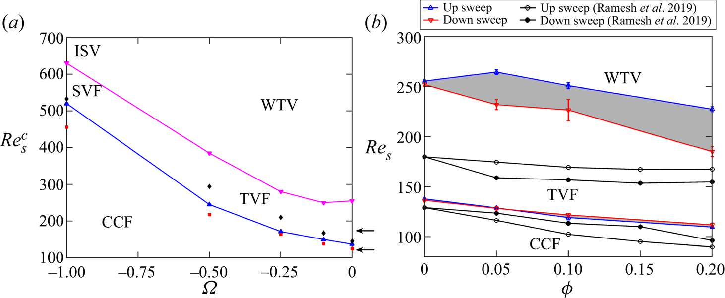
For the particle-free ( $\phi =0$) TCF, figure 2(a) displays the up-sweep data on critical shear Reynolds numbers
 $\mbox {Re}_s^{c1}\ {\rm and}\ \mbox {Re}_s^{c2}$ for primary (
 ${\rm CCF}\to {\rm TVF}$ or
 ${\rm CCF}\to {\rm SVF}$) and secondary (
 ${\rm TVF}\to {\rm WTV}$ or
 ${\rm SVF}\to {\rm ISV}$) transitions, respectively. For a comparison, this figure also includes the data of Andereck et al. (Reference Andereck, Liu and Swinney1986) on
 $\mbox {Re}_s^{c1}\ {\rm and}\ \mbox {Re}_s^{c2}$ (marked by square and diamond symbols) that have been extracted from their figure 2 (see figure 1b). Our estimates of
 $\mbox {Re}_s^{c1}$ are slightly larger but in good agreement with those of Andereck et al. (Reference Andereck, Liu and Swinney1986) at
 $\varOmega \geq -0.5$, but a large quantitative difference is found at
 $\varOmega = -1$, for which the primary bifurcation yields an oscillatory state (SVF). In general, the onset of travelling vortices is delayed significantly (e.g.
 $\mbox {Re}_s^{c2}>\mbox {Re}_s^{c2}|_{ALS}$) for all
 $\varOmega$ in the present set-up.
(a) Critical shear Reynolds number (see (3.1)) for primary (blue line) and secondary (magenta line) transitions in particle-free ( $\phi =0$) TCF at
 $\varOmega < 0$; see text for details. While the red squares and black diamonds denote the (up-sweep) data of Andereck et al. (Reference Andereck, Liu and Swinney1986) for primary and secondary transitions, respectively, the blue and magenta triangles refer to the corresponding data of the present experiments; two arrows mark the data of Ramesh et al. (Reference Ramesh, Bharadwaj and Alam2019) for
 $\varOmega =0$. (b) Phase diagram of patterns in the
 $(\mbox {Re}_s(\phi ), \phi )$-plane at
 $\varOmega \equiv \omega _o/\omega _i=-10^{-3}\approx 0$ and its comparison with Ramesh et al. (Reference Ramesh, Bharadwaj and Alam2019) for
 $\varOmega =0$, marked by circles and black lines. For all cases, the ramping rate is
 ${\rm d}\mbox {Re}(\phi )/{\rm d}\tau _d=0.05$.

Note that the delayed transition to oscillatory states in a small aspect ratio TC cell ( $\varGamma =11$) was confirmed by Ramesh et al. (Reference Ramesh, Bharadwaj and Alam2019) at
 $\varOmega =0$ (see their table 2); their data on the first two critical Reynolds numbers,
 \begin{equation} (\mbox{Re}_s^{c1}, \mbox{Re}_s^{c2}) =\frac{2}{(1+\eta)}\,(\mbox{Re}_i^{c1},\mbox{Re}_i^{c2}) \approx (128, 180), \end{equation}
marked by two arrows on the right of figure 2(a), are in relatively better agreement with the present data than with Andereck et al. (Reference Andereck, Liu and Swinney1986). Although the radius ratio and curvature  $(\eta,\kappa )=(0.891, 0.122)$ of our TC cell are close to
 $(\eta,\kappa )=(0.883, 0.132)$ of Andereck et al. (Reference Andereck, Liu and Swinney1986), the present aspect ratio (
 $\varGamma =8.46$ versus
 $\varGamma _{ALS}=30$) is approximately
 $3.55$ times less than that in the latter work. This axial constraint is known to make the Ekman vortices (Coles Reference Coles1965) stronger in a small-
 $\varGamma$ TC cell, which imparts an overall stabilizing effect (Cole Reference Cole1976; Benjamin Reference Benjamin1978b; Lorenzen, Pfister & Mullin Reference Lorenzen, Pfister and Mullin1983; Mullin, Heise & Pfister Reference Mullin, Heise and Pfister2017; Gopan & Alam Reference Gopan and Alam2020; Aghor & Alam Reference Aghor and Alam2021), thereby delaying the onset of oscillatory modes (WTV/SVF).
Notwithstanding the quantitative differences, we conclude that the present set-up identifies the onset of both primary and secondary states in the counter-rotation regime of the particle-free TCF of an incompressible Newtonian fluid.
3.3.2. Suspension TCF with rotating inner cylinder
It should be noted that the present twin-drive MCR-702 rheometer can be operated smoothly by giving a small amount of rotation to the outer cylinder; we have verified that the torque response fluctuates if the outer cylinder rotation is set to zero ( $\varOmega =\omega _o/\omega _i=0$). Experiments have been conducted at speed ratio
 $\varOmega =\omega _o/\omega _i=-10^{-3}\approx 0$, which represents approximately the case of pure inner-cylinder rotation as studied previously (Majji et al. Reference Majji, Banerjee and Morris2018; Ramesh et al. Reference Ramesh, Bharadwaj and Alam2019). Note that for the particle-free case, the data presented in figure 2(a) at
 $\varOmega =0$ represent speed ratio
 $\varOmega =- 10^{-3}$.
Figure 2(b) shows the phase-diagram of patterns in the ( $\mbox {Re}_s,\phi$)-plane at
 $\varOmega =-10^{-3}\approx 0$ for a ramping rate
 ${\rm d}\mbox {Re}(\phi )/{\rm d}\tau _d=0.05$; the up- and down-sweep data on (
 $\mbox {Re}_s^{c1}, \mbox {Re}_s^{c2}$) of Ramesh et al. (Reference Ramesh, Bharadwaj and Alam2019) are also superimposed for comparison. It is seen that while the critical Reynolds number for primary bifurcation is slightly larger than that of Ramesh et al. (Reference Ramesh, Bharadwaj and Alam2019), the secondary bifurcation to oscillatory states is delayed significantly for all
 $\phi \leq 0.2$ in the present set-up. Comparing with the data obtained from figure 12(b) of Ramesh et al. (Reference Ramesh, Bharadwaj and Alam2019), we find that their up-sweep value
 $\mbox {Re}_s^{c2}(\phi =0.2,\varOmega =0) =2\mbox {Re}_i/(1+\eta )\approx 180$ for
 $\varGamma \approx 8.4$ is very close to the down-sweep value
 $\mbox {Re}_s^{c2}(\uparrow, \downarrow ) =(220, 180)$ found in the present experiments. The delayed transition to the oscillatory secondary state (in comparison to previous works: Majji et al. Reference Majji, Banerjee and Morris2018; Ramesh et al. Reference Ramesh, Bharadwaj and Alam2019) may be attributed to (i) a smaller aspect ratio TC set-up, and (ii) a relatively wider distribution of the particle size.
A crucial difference in the present results for the inner-cylinder rotation case ( $\varOmega \approx 0$) compared with Ramesh et al. (Reference Ramesh, Bharadwaj and Alam2019) is the absence of non-axisymmetric states (such as spiral vortices) as the primary bifurcation state from the CCF regime – this issue has been resolved by carrying out experiments at much smaller ramping rates; see § 6.1. In the remaining part of this paper, we explore the effect of counter-rotation (
 $\varOmega < 0$) on the emerging patterns such as in figures 2(a) and 2(b) by considering a non-colloidal suspension of neutrally buoyant particles.
4. Results for  $\varOmega \geq -0.5$: oscillatory and quasi-periodic states and their multiplicity

Moving onto suspensions ( $\phi \leq 0.2$) under counter-rotation, experiments have been conducted for four different values of the rotation ratio
 $\varOmega =\omega _o/\omega _i=-0.1$,
 $-0.25$,
 $-0.5$ and
 $-1.0$, along with the case of a rotating inner cylinder (
 $\varOmega =-10^{-3}\approx 0$). The results for
 $\varOmega =-0.25$,
 $-0.1$ and
 $-0.5$ are discussed in § 4.1 and § 4.2, respectively, that lead to wavy and modulated wavy vortices, with the latter being a quasi-periodic state. A separate section (§ 5) is devoted to discussing results for
 $\varOmega =-1$ that give birth to spiral vortices and their interacting twins.
4.1. ${\rm CCF}\leftrightarrow {\rm TVF}\leftrightarrow {\rm WTV}$ transition, multiroll states, and wave speed at $\varOmega \geq -0.25$


Since the transition sequence is found to be the same ( ${\rm CCF}\to {\rm TVF}\to {\rm WTV}$) for rotation ratios
 $\varOmega =-0.25$ and
 $-0.1$, most of the results will be presented for
 $\varOmega =-0.25$, which include (i) image analyses, (ii) spectral characterization of patterns, and (iii) the torque data. We summarize our findings on (i) the phase diagrams in § 4.1.1, followed by (ii) the evidence of multiroll transition and its characterization in § 4.1.2, and (iii) an analysis of the dominant frequency of the wavy vortices in § 4.1.3.
4.1.1. Phase diagram of patterns
Figures 3(a,b) display the phase diagrams of patterns in the  $(\mbox {Re}_s, \phi )$-plane for
 $\varOmega =-0.1$ and
 $-0.25$, respectively. In each panel, the blue (with up-triangles) and red (with down-triangles) lines represent the onset/critical values of
 $\mbox {Re}_s^{cj}$ during up-sweep and down-sweep runs, respectively, with the grey-shaded regions representing hysteresis. For both
 $\varOmega =-0.1$ and
 $-0.25$, the sequence of bifurcations with increasing
 $\mbox {Re}_s$ is found to be
 ${\rm CCF}\to {\rm TVF}\to {\rm WTV}$ states at any
 $\phi \leq 0.2$. Note that for the range of
 $\mbox {Re}_s(\phi )$ explored (with
 $f_{max}=20$ Hz, marked by the lower boundary of the hatched zone in each panel of figure 3), the transitions up to the secondary state (WTV) have been found at
 $\varOmega \geq -0.25$.
Phase diagram of patterns in the  $(\mbox {Re}_s(\phi ), \phi )$-plane at
 $\varOmega \equiv \omega _o/\omega _i$ values (a)
 $-0.1$, and (b)
 $-0.25$. Approximate boundaries for primary (
 ${\rm CCF}\to {\rm TVF}$) and secondary (
 ${\rm TVF}\to {\rm WTV}$) bifurcations are marked from up-sweep (blue lines, with up-triangles) and down-sweep (red lines, with down-triangles) runs; the ramping rate is
 ${\rm d}\mbox {Re}(\phi )/{\rm d}\tau _d=0.05$. The dashed and dotted black lines represent the loci of multiroll transitions (between different number of rolls/vortices); see the text in § 4.1.2 for related details.

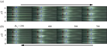
Snapshots at different values of  $\mbox {Re}_s$ during (a) up-sweep, and (b) down-sweep runs. Outward jets (surrounded by two inward jets) are marked sequentially from the bottom, indicating changes in the numbers of rolls/vortices during up-sweep and down-sweep runs. Parameter values are
 $\varOmega =-0.25$,
 $\phi =0$ and
 ${\rm d}\mbox {Re}(\phi )/{\rm d}\tau _d=0.05$.

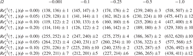
Figures 3(a,b) illustrate that there is a global stabilization of the flow with increasing counter-rotation ratio  $\varOmega <0$; see also the tabulated data in Appendix A. Our primary result is that for specified
 $\varOmega$, the effect of particle loading
 $\phi$ is to decrease the critical values of the shear Reynolds numbers
 $\mbox {Re}_s^{c1}$ and
 $\mbox {Re}_s^{c2}$, implying a destabilizing effect of particles on the onset of primary (TVF) and secondary (WTV) states. The second result is that the destabilizing effect of particles on primary bifurcation increases at larger values of
 $|\varOmega |$ since
 $({\rm d}Re_s^{c1}/{\rm d}\phi )|_{\varOmega =-0.25}> ({\rm d}Re_s^{c1}/{\rm d}\phi )|_{\varOmega =-0.1}$, which can be verified from the data presented in Appendix A. Third, the primary bifurcations at
 $\varOmega =-0.1$ (figure 3a) and
 $\varOmega =-0.25$ (figure 3b) are largely devoid of hysteresis, i.e.
 \begin{equation} \Delta\mbox{Re}_s^{c1}={\mbox{Re}_s^{c1}}_{\uparrow} - {\mbox{Re}_s^{c1}}_{\downarrow}\approx 0, \end{equation}
for  $\phi \leq 0.2$. Finally, regarding the secondary transition
 ${\rm TVF}\to {\rm WTV}$ in figures 3(a,b), a comparison with figure 2(b) indicates that the degree of hysteresis,
 \begin{equation} \Delta\mbox{Re}_s^{c2}={\mbox{Re}_s^{c2}}_{\uparrow} - {\mbox{Re}_s^{c2}}_{\downarrow}, \end{equation}
over which the primary and secondary states coexist, decreases with increasing counter-rotation  $|\varOmega |$.
4.1.2. Multiroll transition: merging and splitting of vortices and the torque data
The dashed and dotted lines in figures 3(a,b) refer to the transitions between different numbers of vortices, as explained below. Focusing on figure 3(b), we display a series of four snapshots ( $\mbox {Re}_s=250, 400, 500$ and
 $700$) in figure 4 during up-sweep (figure 4a) and down-sweep (figure 4b) runs for the particle-free (
 $\phi =0$) case, with rotation ratio
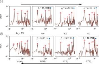
 $\varOmega =-0.25$. The corresponding temporal power spectra (over a time period of
 $5$ s), averaged at two axial locations
 $z/\delta =3.2$ and
 $5.4$ (marked by square boxes in each image in figure 4), are displayed in figure 5. The latter figure confirms that the image at
 $\mbox {Re}_s=250$ represents a stationary mode (TVF), whereas the images at
 $\mbox {Re}_s=400$, 500 and
 $750$ represent oscillatory wavy vortices (WTV) that travel along the azimuthal direction with a frequency as marked by a blue circle in each plot of figure 5. Note that the calculated dominant frequency is always below the Nyquist criterion (i.e.
 $f < f_{Nyq}\equiv f_{acq}/2$, where
 $f_{acq}=60$ Hz is the acquisition frequency); we have ensured that the frequency data presented for all oscillatory modes in this paper satisfy the Nyquist criterion (Nyquist Reference Nyquist1932).
Temporal power spectra of images in figure 4; for each image, the mean FFT of the scattered light intensity is calculated by averaging over two square boxes (marked in figure 4) of  $30\times 30$ pixels, located at axial locations
 $z/\delta =3.2$ and
 $5.4$, over a time window of
 $2.5$ s; see § 2.3 for details. The blue circle marks the dominant frequency of the WTV; the up- and down-triangles mark
 $f_\triangle =f_o$ and
 $f_{\nabla }=f_i$, respectively, and their harmonics. Note that the diamond symbol marks a constant frequency
 $f_\diamond \approx 19.3$ Hz (which appears due to the presence of two AC tube lights); this non-physical mode disappeared from the power spectrum when the images were captured with AC lights switched off.

Returning to figure 4, we note that each snapshot represents a cropped image up to axial height  $z/\delta \approx 6.83$. The top part of the TC cell is covered with a plexiglas lid of height
 $h_{lid}/\delta \approx 1.6$, with a very thin Teflon tape being used for tightening the lid around the outer cylinder; the camera is focused just below the lid to avoid reflections. Therefore, one has to focus on the lower half (up to
 $z/\delta \approx 4.2$) of the TC cell and multiply it by two to estimate approximately the number of vortices along the axial direction. For example, in the leftmost images in figure 4 (i.e.
 $\mbox {Re}_s=250$), the numbers of Taylor vortices are
 $8$ and
 $10$, respectively, during up- and down-sweep runs; similarly, the number of wavy vortices at
 $\mbox {Re}_s=700$ (the rightmost images) are
 $6$ and
 $8$ during up- and down-sweep runs, respectively; however, only a 6-roll state is found at
 $\mbox {Re}_s=500$. The axial height of vortices has been verified by calculating the spatial Fourier transform of the scattered light intensity along a vertical strip (not shown). On the whole, figure 4 confirms that a state (TVF or WTV) with different number of vortices can be realized at a given Reynolds number
 $\mbox {Re}_s$ depending on the ramping protocol. The transition of a state having different numbers of rolls/vortices, leading to multiplicity of states, is referred to as multiroll transition (Benjamin Reference Benjamin1978b; Mullin et al. Reference Mullin, Heise and Pfister2017; Gopan & Alam Reference Gopan and Alam2020, Reference Gopan and Alam2021; Aghor & Alam Reference Aghor and Alam2021). This finding may be juxtaposed with the fact that the primary bifurcation is expected to yield an 8-roll state for the case of inner-cylinder rotation (such that the vortex size scales approximately with the annular gap
 $\delta$) since the aspect ratio of the present TC cell is
 $\varGamma =h/\delta \approx 8.46$.
To identify the range of  $\mbox {Re}_s(\phi,\varOmega )$ over which the multiroll transition occurs, we show (i) the space–
 $\mbox {Re}_s(\phi )$ diagrams and (ii) the frequency (
 $\omega /\omega _i, \mbox {Re}_s$) maps in the upper and middle images of figures 6(a,b) for up-sweep and down-sweep runs, respectively, for
 $\phi =0$; the analogous plots for
 $\phi =0.1$ are displayed in the respective images of figures 6(c,d). While the space–
 $\mbox {Re}_s$ diagrams confirm that the merging and splitting of vortices give birth to different number of roll configurations, leading to (i)
 $6\leftrightarrow 8\leftrightarrow 10$ rolls at
 $\phi =0$, and (ii)
 $6\leftrightarrow 8$ rolls at
 $\phi =0.1$, the (
 $\omega /\omega _i, \mbox {Re}_s$) maps mark the onset of oscillatory (
 $\omega \neq 0$) states and thereby help to identify the location of the critical Reynolds number
 $\mbox {Re}_s^{c2}(\phi )$ at the secondary transition (
 ${\rm TVF}\leftrightarrow {\rm WTV}$). Note in the middle plots of figures 6(a–d) that the dominant frequency of WTV undergoes an abrupt jump when a WTV state degenerates into another WTV state with a different number of rolls – this can be used as a metric to identify roll transitions in the oscillatory regimes (such as WTV and MWV).
Space– $\mbox {Re}_s(\phi )$ plots (top) of patterns (showing vortex merging and splitting phenomena), the normalized frequency
 $\omega /\omega _i$ versus
 $\mbox {Re}_s$ (middle), and the effective Nusselt number
 $\mbox{Nu}_\omega$ versus
 $\mbox {Re}_s$ (bottom) for up-sweep (left) and down-sweep (right) runs at (a,b)
 $\phi =0$ and (c,d)
 $\phi =0.1$. In the bottom images of (b,d), the up-sweep torque data are superimposed as magenta curves; the grey-shaded regions denote the hysteresis loops for
 $6\leftrightarrow 8$ roll WTV; see the text for details. The rotation ratio is
 $\varOmega =-0.25$, and the ramping rate is
 ${\rm d}\mbox {Re}(\phi )/{\rm d}\tau _d=0.05$.

A robust signature of multiroll transition (for both stationary or oscillatory vortices) can be traced to the torque data measured at the inner cylinder as explained below. In the lower plots in figures 6(a–d), the variations of the effective Nusselt number  $\mbox {Nu}_\omega$ (see (3.11)) with
 $\mbox {Re}_s(\phi )$ are displayed. It is seen that the multiroll transition is accompanied by a sharp jump in
 $\mbox {Nu}_\omega$ that increases/decreases with increasing/decreasing number of vortices in the WTV regime. This implies that the transport of angular momentum from the inner cylinder is enhanced with increasing number of wavy vortices – this observation is similar to the findings of Martínez-Arias et al. (Reference Martínez-Arias, Peixinho, Crumeyrolle and Mutabazi2014) in the context of Taylor vortices in the turbulent regime. The coexistence of
 $6$-,
 $8$- and
 $10$-rolls can be appreciated by superimposing the up- and down-sweep torque data (see figures 6b,d), confirming the existence of three stable states over a large range of
 $\mbox {Re}_s(\phi )$. In particular, the grey-shaded regions in the bottom plots of figures 6(b,d) represent the hysteresis loops for
 $6\leftrightarrow 8$ roll transition; note further that the 8-roll WTV branch of the up-sweep run can be extended smoothly to join with the corresponding
 $\mbox {Nu}_\omega$ branch of the down-sweep run. Note that the latter
 $8$-roll WTV state (of the down-sweep run) that appears at large
 $\mbox {Re}_s$ could be temporally unstable, as confirmed from additional experiments at specified values of
 $\mbox {Re}_s$ over long-enough time
 $O(10^3/f_i)$. Therefore, for both
 $\phi =0$ and
 $0.1$, the
 $6$-roll WTV state seems to be stable at large values of
 $\mbox {Re}_s$ beyond the grey-shaded hysteresis loops in figures 6(b,d).
The multiplicity of states (Benjamin & Mullin Reference Benjamin and Mullin1982) in the nonlinear regime of the TCF is not surprising. For example, Coles (Reference Coles1965) discovered approximately  $25$ WTV states over a range of inner-cylinder Reynolds numbers
 $\mbox {Re}_i$, with each state being characterized by (i) a distinct number of vortices, and (ii) a distinct number of azimuthal waves (i.e. the azimuthal wavenumber). He also clarified that with changing
 $\mbox {Re}_i$, the occurrences of these states are marked by the appearance or disappearance of vortices in pairs (as demonstrated in figure 4) and the addition or subtraction of the number of waves. The role of the finite length of the TC cell (such as in our set-up) on the multiplicity of Taylor vortices was studied carefully by Benjamin via theory (Benjamin Reference Benjamin1978a) and experiments (Benjamin Reference Benjamin1978b). He explained the onset of multiroll transition with increasing
 $\varGamma$ or
 $\mbox {Re}_i$ from the dynamical systems theory in terms of perfect and imperfect bifurcations that refer to periodic and no-slip axial boundary conditions, respectively; his experimental findings were reproduced qualitatively by a low-dimensional model (Schaeffer Reference Schaeffer1980). Subsequent experiments and theory (see Cliffe, Mullin & Schaeffer (Reference Cliffe, Mullin and Schaeffer2012) and references therein), along with the most recent experiments of Mullin et al. (Reference Mullin, Heise and Pfister2017), confirmed that the multiroll transition is not a small aspect ratio phenomenon, but can occur in a large aspect ratio (
 $\varGamma > 40$) TC cell too. In this context, we refer to figures 5 and 6 in Aghor & Alam (Reference Aghor and Alam2021) to understand the coexistence of
 $2$-,
 $4$- and
 $6$-roll TVF states beyond a minimum value of
 $\mbox {Re}$ if the experiments are carried out in a TC cell with an aspect ratio, for example, of around
 $\varGamma = 5$. To our knowledge, the present results on multiroll transitions in the counter-rotation regime are new even for the particle-free (
 $\phi =0$) incompressible TCF, since the latter case has been studied exclusively with a rotating inner cylinder (Benjamin Reference Benjamin1978b; Mullin & Benjamin Reference Mullin and Benjamin1980; Cliffe et al. Reference Cliffe, Mullin and Schaeffer2012; Mullin et al. Reference Mullin, Heise and Pfister2017).
4.1.3. Effects of particle loading on dominant frequency and its possible scaling
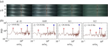
Figure 7 displays a series of snapshots with increasing particle volume fraction  $\phi$ at
 $(\mbox {Re}_s,\varOmega )=(300, -0.25)$; figure 3(b) confirms that
 $\mbox {Re}_s(\phi )=300$ refers to the WTV state for all
 $\phi \leq 0.2$. The visual inspection of waves in figure 7 indicates that the effect of increasing particle loading is to decrease the amplitude of wavy vortices; however, their wavelength seems to remain unchanged up to
 $\phi \leq 0.1$, and increases at
 $\phi =0.2$ for these parameter values. The fundamental frequency of wavy vortices (
 $f_{wv}=f_1=\omega _1/2{\rm \pi}$), determined from the power spectrum of the scattered light intensity, is marked by a blue circle in figure 7(b). We find a non-monotonic dependence of the dimensional
 $f_{1}$ on
 $\phi$ for given
 $\mbox {Re}_s$; however, the normalized frequency is
 $\omega _1/\omega _r= 2.08, 2.09, 2.15, 0.64$ at
 $\phi =0, 0.05,0.1, 0.2$, with the relative frequency of the two cylinders being
 $f_r=\omega _r/2{\rm \pi} = 9.56,11.22,13.92,22.12$ Hz. The sharp decrease of the fundamental mode
 $\omega _1$ at
 $\phi =0.2$ is likely due to the increased wavelength of wavy vortices at
 $\phi =0.2$, which is visible in figure 7(a).
Effects of particle volume fraction on wavy vortices (a) and the power spectra (b) at  $\mbox {Re}_s(\phi )=300$ and
 $\varOmega =-0.25$. The dominant frequency (
 $f_1$ in Hz) is marked by a blue circle in each plot (with the grey cross being its harmonic), and the up- and down-triangles represent the rotation speed of the inner and outer cylinders, respectively. For each
 $\phi$, the mean FFT of the scattered light intensity is calculated by averaging over two square boxes (marked in each image) of
 $30\times 30$ pixels over a time window of
 $5$ s. All data refer to an up-sweep run at ramping rates of
 ${\rm d}\mbox {Re}(\phi )/{\rm d}\tau _d=0.05$ (
 $\phi \leq 0.1$) and
 $0.02$ (
 $\phi =0.2$).

Variations of the scaled fundamental frequency of wavy vortices,  $\omega _1/\omega _r$, with (a)
 $\mbox {Re}_s(\phi )$ and (b)
 $\mbox {Re}_s(0)=\mbox {Re}_s(\phi )\,\mu _r$, where
 $\mu _r$ is the relative viscosity of the suspension, and
 $\omega _r=|\omega _i-\omega _o|$ is the relative angular speed of the two cylinders, for
 $\varOmega =-0.25$ (up-sweep run). The data for
 $\phi =0.2$ refer to ramping rate
 ${\rm d}\mbox {Re}(\phi )/{\rm d}\tau _d=0.02$ (the SVF state was found over
 $\mbox {Re}_s\in (140,146)$; see § 6.1), while those for
 $\phi \leq 0.1$ represent
 ${\rm d}\mbox {Re}(\phi )/{\rm d}\tau _d=0.05$.

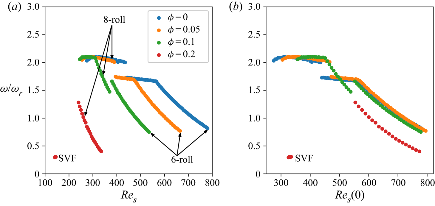
Figure 8(a) displays the variations of the normalized frequency  $\omega _1/\omega _r$ with the shear Reynolds number
 $\mbox {Re}_s(\phi )$ for different
 $\phi$ at
 $\varOmega =-0.25$; we have plotted only the up-sweep data, for which the
 $\omega$ branches with
 $6$- and
 $8$-roll states are also marked. It is clear from this figure that the jumps in
 $\omega _1/\omega _r$ are tied to the onset of multiroll transitions as confirmed also from (i) the space–time and frequency maps in figures 6(a,c), and (ii) the phase diagram in figure 3(b). In general,
 $\omega _1/\omega _r$ decreases with increasing
 $\mbox {Re}_s$ for a given
 $\phi$, a trend that agrees with the wave speed data presented in figure 5 of King et al. (Reference King, Li, Lee, Swinney and Marcus1984) for the particle-free case. Concerning the large values of
 $\omega _1/\omega _i> 2$ near the onset of the WTV, a comparison with the data in figure 6 of Andereck et al. (Reference Andereck, Liu and Swinney1986) is pertinent. They reported a dominant wavy mode at
 $\omega _1/\omega _i \approx 2$ for
 $(\mbox {Re}_s, \varOmega )=(475, -0.277)$ that compares well with our data within the plateau region at
 $\mbox {Re}_s\in (300, 500)$ in figure 8(a).
The data of figure 8(a) are replotted in terms of  $\mbox {Re}_s(0)$ in figure 8(b); note that
 $\mbox {Re}_s(0)=\mu _r\,\mbox {Re}_s(\phi )$ is the shear Reynolds number based on the fluid viscosity
 $\mu _l=\mu (0)$, and
 $\mu _r(\phi )$ is the relative viscosity (2.2) of the suspension. It is seen that the normalized frequency data collapse on two different curves for
 $6$- and
 $8$-roll states, irrespective of the value of
 $\phi$, indicating that
 $\mbox {Re}_s(0)$ could be the relevant scaling variable for the speed data. The dependence of the dominant frequency
 $\omega _1$ on the number of rolls suggests that the frequency
 \begin{equation} \omega_1 = \omega_1\left(\mbox{Re}_s(0), \lambda_z\right) \equiv \omega_1\left(\mu_r\,\mbox{Re}_s(\phi), \lambda_z\right) \end{equation}
of wavy vortices would also depend on the axial wavelength  $\lambda _z$ of vortices in addition to
 $\mbox {Re}_s(0)$. Figure 8(b) illustrates further that for a given
 $\mbox {Re}_s(0)$,
 $\omega _1/\omega _r$ is smaller in the
 $8$-roll state than in the
 $6$-roll state in the decaying region of
 $\omega _1/\omega _r$, while the opposite trend is found in the plateau region of
 $\omega _1/\omega _r$ that occurs near the onset of WTV (i.e. just above
 $\mbox {Re}_s=\mbox {Re}_s^{c2}$). We conclude that the normalized frequency
 $\omega _1/\omega _r$ of wavy vortices may decrease or increase with increasing
 $\lambda _z$ depending on the value of
 $\mbox {Re}_s$. Indeed, such a non-monotonic dependence of the wave speed on
 $\lambda _z$ was reported (see figure 4 of King et al. Reference King, Li, Lee, Swinney and Marcus1984) in the context of particle-free incompressible TCF. We note in passing that the wave speed
 $v_\theta$ and the passage frequency
 $f_{wv}=\omega _1/2{\rm \pi}$ are tied to each other via
 $v_\theta =f_{wv}\lambda _\theta$, with
 $\lambda _\theta$ being the azimuthal wavelength of wavy vortices.
4.2. Results for $\varOmega =-0.5$: emergence of quasi-periodic states

4.2.1. MWV flow and its spectral characteristics
For rotation ratio  $\varOmega =-0.5$ (see figure 1b), figure 9 displays structural information on wavy vortices for
 $\mbox {Re}_s(\phi )=600$ (figures 9a,c),
 $\mbox {Re}_s(\phi )=640$ (figure 9b) and
 $\mbox {Re}_s(\phi )=800$ (figure 9d); figures 9(a,b) represent
 $\phi =0.1$, and figures 9(c,d) represent
 $\phi =0$. Each panel consists of a snapshot at top left and its time evolution over
 $2.5$ s at top right, along with its temporal (bottom left) and spatial (bottom right) power spectra. In each frequency plot (PSD versus
 $f/f_i$ or
 $\omega /\omega _i$), the blue circle, orange star and green triangle represent frequencies of propagating patterns, whereas the grey cross represents a harmonic of propagating modes; on the other hand, the peaks marked by the red down and up triangles, respectively, denote inner and outer cylinder rotation frequencies (i.e.
 $f_\triangle =f_o$ and
 $f_{\nabla }=f_i$) and their harmonics, whereas the red diamond refers to a non-physical mode (
 $f_{\diamond }\approx 19.3$ Hz) as mentioned in the caption of figure 5.
Each panel shows a snapshot of wavy vortices (top left) and its time evolution over  $2.5$ s (top right), and two power spectra of scattered light intensity
 $I(z,t)$ (bottom): mean temporal FFT (bottom left) averaged over two axial locations at
 $z/\delta = 3.2$ and
 $5.4$ (marked by black squares in each snapshot), and spatial FFT (bottom right) along a vertical strip, marked by the red dashed line in each image, of width
 $1$ pixel; see the text in § 2.3 for details on FFT analyses. While the blue circle in each temporal FFT plot represents the frequency of the dominant mode (WTV), the orange star and green triangle represent low-frequency modulations (and hence an MWV state) of the dominant wavy mode; the grey crosses represent the harmonics of the above modes. The filled green circles in each spatial FFT plot denote the axial wavelength of vortices and their modulations, whereas the open red circles represent the axial periodicity due to cropped images as mentioned in § 2.3. Parameter values are
 $\varOmega =-0.5$ and: (a,c)
 $\mbox {Re}_s(\phi )=600$, (b)
 $\mbox {Re}_s(\phi )=640$, and (d)
 $\mbox {Re}_s(\phi )=800$, with (a,b)
 $\phi =0.1$ and (c,d)
 $\phi =0$. All data refer to up-sweep runs at ramping rate
 ${\rm d}\mbox {Re}(\phi )/{\rm d}\tau _d=0.05$.

Note that the lower left plot of figure 9(a) for  $(\mbox {Re}_s, \phi )=(600, 0.1)$ contains a sharp peak at
 $\omega _1/\omega _i \approx 0.945$ (marked by a blue circle) along with a low-frequency mode at
 $\omega _2/\omega _i\approx 0.45$ (orange star), while the analogous plot for
 $\phi =0$ in figure 9(c) contains a single peak at
 $\omega _1/\omega _i\approx 1.375$. Therefore, the pattern in figure 9(c) represents a singly periodic wave, called the wavy Taylor vortex, whereas figure 9(a) represents a doubly periodic wave (Donnelly et al. Reference Donnelly, Park, Shaw and Walden1980; Gorban, Swinney & Rand Reference Gorban, Swinney and Rand1981; Gorban & Swinney Reference Gorban and Swinney1982; Coughlin & Marcus Reference Coughlin and Marcus1992; Takeda Reference Takeda1999), called the modulated wavy vortex. The basic characteristic distinction of MWV is tied to the appearance of a low (incommensurate) frequency mode (and hence called a doubly periodic wave) that was clarified by Gorban & Swinney (Reference Gorban and Swinney1982) and most recently by Dutcher & Muller (Reference Dutcher and Muller2009). Note that the emergence of an incommensurate frequency with increasing
 $\mbox {Re}_i$ (and hence the onset of MWV) was first detected by Gollub & Swinney (Reference Gollub and Swinney1975) in the context of the TCF with a rotating inner cylinder.
In the counter-rotation regime of TCF, Andereck et al. (Reference Andereck, Liu and Swinney1986) confirmed further that there could be a third frequency (at  $\omega _3 < \omega _2$) in MWV that refers to axial-phase oscillation. Returning to figure 9(b), we note the presence of a third frequency (marked by a green triangle) and its harmonic (grey cross) at
 $\omega _3/\omega _i\approx (0.305, 0.61)$ for
 $\phi =0.1$ – this is in addition to two (incommensurate) fundamental modes at
 $(\omega _1,\omega _2)/\omega _i=(0.91, 0.415)$. Therefore, figure 9(b) indeed represents a triply periodic wave in suspension TCF, analogous to the one discussed in figure 5 of Andereck et al. (Reference Andereck, Liu and Swinney1986). On the other hand, for the particle-free case at
 $\mbox {Re}_s=800$, only two frequencies
 $(\omega _1,\omega _2)/\omega _i \approx (0.82, 0.363)$, with a harmonic of the fundamental mode at
 $\omega _h=2\omega _1\approx 1.62$ (marked by a grey cross), are seen in the power spectrum in figure 9(d).
In each spatial spectrum plot in the lower right plots of figures 9(a–d), the dominant peak (marked by filled green circles) is located at  $\delta /\lambda \approx 0.88$, indicating that the axial wavelength of MWV scales approximately with the annular gap (
 $\delta$); note that the red-circled peaks represent the periodicity due to the stitching of
 $N=300$ (see § 2.3) images axially. For the case
 $\phi =0.1$ in figures 9(a,b), the sub-dominant peaks appear at
 $\delta /\lambda \sim 0.5\ {\rm and}\ 1.03$ that correspond to spatial modulations of MWV. Similar structural features can be ascertained from figure 9(d), which represents an MWV state for the particle-free (
 $\phi =0$) case.
For both WTV and MWV states, the fundamental mode  $\omega _1$ listed in table 1 corresponds to the ‘passage’ frequency of waves along the azimuthal direction at a given location. Table 1 indicates that
 $\omega _1$ (normalized by the relative angular speed
 $\omega _r=|\omega _i-\omega _o|$) decreases with increasing
 $\mbox {Re}_s$, and the effect of particle loading (
 $\phi >0$) is to decrease the passage frequency of both MWV and WTV as well. These overall findings on the effect of
 $\phi, \mbox {Re}_s$ on
 $\omega _1$ mirror those for the WTV state at
 $|\varOmega |\leq -0.25$, as discussed for figure 8 in § 4.1.3. Collectively, the decreasing trend of the dominant frequency with increasing
 $\mbox {Re}_s$ in figure 8 and table 1 is similar to the experimental (King et al. Reference King, Li, Lee, Swinney and Marcus1984; Andereck et al. Reference Andereck, Liu and Swinney1986) and theoretical (Jones Reference Jones1982) findings in the WTV regime. In addition, table 2 in Andereck et al. (Reference Andereck, Liu and Swinney1986) indicates that
 $\omega _1/\omega _r$ depends weakly on both azimuthal and axial wavenumbers of wavy vortices – such detailed characterizations are beyond the scope of the present paper.
Variation of the dimensionless dominant frequency  $\omega _k/\omega _r$ of WTV and MWV states with
 $\mbox {Re}_s(\phi )$ at
 $\varOmega =-0.5$, where
 $\omega _r=|\omega _i-\omega _o|$ is the relative angular speed between the two cylinders; note that
 $k=1$ refers to the frequency (
 $\omega _1$) of wavy vortices, but
 $k=1,2,3$ for MWV such that
 $\omega _1>\omega _2>\omega _3$, with
 $\omega _1$ representing the fundamental wavy mode. All data refer to up-sweep runs at ramping rate
 ${\rm d}\mbox {Re}(\phi )/{\rm d}\tau _d=0.05$.

4.2.2. Phase diagrams and flow multiplicity in MWV regime
Figures 10(a,b) summarize different patterns in the  $(\mbox {Re}_s(\phi ), \phi )$-plane at
 $\varOmega =-0.5$ for up-sweep and down-sweep experiments, respectively. For both runs, we find that while the primary bifurcation yields a stationary TVF state at
 $\mbox {Re}_s\geq \mbox {Re}_s^{c1}$ (marked by the lowest phase boundary in each panel), the tertiary bifurcation yields MWV, such as those described in figures 9(a,b,d), at
 $\mbox {Re}_s\geq \mbox {Re}_s^{c3}$ (marked by the uppermost phase boundary in each panel). Interestingly, the patterns lying between the TVF and MWV regions can appear in the form of (i) WTV, such as in figure 9(c), and/or (ii) two different variants of modulated waves (MWV
 $_1$ and MWV
 $_2$; see § 4.2.3 for their characterization). The MWV state is expected to lead to a chaotic state (Fenstermacher, Swinney & Gollub Reference Fenstermacher, Swinney and Gollub1979; Gorban & Swinney Reference Gorban and Swinney1982; Andereck et al. Reference Andereck, Liu and Swinney1986; Coughlin & Marcus Reference Coughlin and Marcus1992; Takeda Reference Takeda1999; Dutcher & Muller Reference Dutcher and Muller2009) at higher values of
 $\mbox {Re}_s$ (see figure 1a).
Phase diagram of patterns in the  $(\mbox {Re}_s(\phi ), \phi )$-plane at
 $\varOmega =-0.5$: (a) up-sweep and (b) down-sweep runs. While the phase boundary for primary (
 ${\rm CCF}\to {\rm TVF}$) bifurcation has been obtained from both the space–time maps of images and the torque data, phase boundaries for secondary (
 ${\rm TVF}\to {\rm WTV}/{\rm MWV}_1$) and higher-order (
 ${\rm WTV}\to {\rm MWV}$ or
 ${\rm MWV}_1\to {\rm WTV}$ or
 ${\rm MWV}_1\to {\rm MWV}_2$) bifurcations have been determined from the frequency analyses. The ramping rate is
 ${\rm d}\mbox {Re}(\phi )/{\rm d}\tau _d=0.05$, except for the MWV
 $_1$ state at
 $\phi =0.05$, for which the experiments were carried out with
 ${\rm d}\mbox {Re}(\phi )/{\rm d}\tau _d=0.025$.

Note that figures 10(a,b) have been drawn by analysing data from a particular set of UD experiments with  ${\rm d}\mbox {Re}(\phi )/{\rm d}\tau _d=0.05$. Analysing different experimental runs, we verified that the transition boundaries for primary (
 ${\rm CCF}\to {\rm TVF}$) and secondary (from TVF to WTV or MWV
 $_1$) states do not vary noticeably with changing ramping rate if
 ${\rm d}\mbox {Re}(\phi )/{\rm d}\tau _d\leq 0.05$. However, (i) the location of the transition boundary to the MWV state and/or (ii) the range of
 $\mbox {Re}_s$ over which the WTV/MWV
 $_1$/MWV
 $_2$ states persist seems to depend on the ramping rate and the ramping protocols as discussed in § 6.2.
The dotted lines in figure 10(b) correspond to transitions between different number of roll configurations (as marked in its legend) in the MWV, WTV and TVF regimes. As in the case of TVF and WTV states in figure 6, the merging and splitting of vortices are responsible for the genesis of multiroll states in the MWV regime too; similarly, the jumps in (i)  $\mbox {Nu}_\omega$ and (ii) the frequency (
 $\omega _1, \omega _2$) are found at the onset of
 $8\leftrightarrow 10$ roll MWV states – the related details are omitted for the sake of brevity.
4.2.3. Different variants of modulated waves
The regimes of two variants of modulated waves (MWV $_1$ and MWV
 $_2$) are marked by green and blue-shaded regions in figures 10(a,b), respectively. The MWV
 $_1$ and MWV
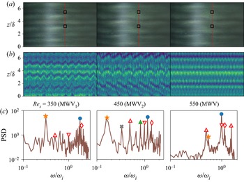
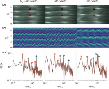
 $_2$ states differ from the MWV state (such as in figures 9a,b,d), which can be appreciated from figure 11 which displays images, space–time maps and power spectra at
 $\mbox {Re}_s=350$,
 $450$ and
 $550$ for the down-sweep run with
 $\phi =0.1$. While the MWV
 $_1$ state is characterized by two frequencies (
 $\omega _1,\omega _2$), the power spectrum of MWV
 $_2$ contains an additional sharp peak, close to the fundamental mode
 $\omega _1$, marked by the green triangle, see figure 11(c). For both MWV
 $_1$ and MWV
 $_2$, the (broad) low-frequency peak
 $\omega _2$ (marked by an orange star) is the dominant one that has visible footprints in the respective space–time maps in terms of low-frequency and long-wave modulations. The latter spatio-temporal modulations are markedly different from those of the standard MWV state (that appear at relatively large
 $\mbox {Re}_s$) as seen in the rightmost parts of figure 11.
Different variants of MWV during down-sweep runs at  $\phi =0.1$ with
 ${\rm d}\mbox {Re}(\phi )/{\rm d}\tau _d=0.05$: (a) images, (b) space–time maps over
 $2.5$ s, and (c) power spectrum: MWV
 $_1$ (
 $\mbox {Re}_s=350$), MWV
 $_2$ (
 $\mbox {Re}_s=450$) and MWV (
 $\mbox {Re}_s=550$); refer to the phase diagram in figure 10(b) for the range of
 $\mbox {Re}_s(\phi )$ over which different states exist.

Similar spatio-temporal characteristics of the MWV $_1$ state persist during up-sweep runs, see the left-hand parts of figure 12 for
 $\phi =0$ (figures 12a,b) and
 $\phi =0.1$ (figures 12c,d). For these cases too, the low-frequency peak (marked by an orange star) contains the maximal energy and hence dictates the structural modulations of wavy vortices. An interesting finding in figures 12(a–d) is a novel transition sequence
 ${\rm TVF}\to {\rm MWV}_1\to {\rm WTV}\to {\rm MWV}$, in which a stationary state (TVF) gives birth to a two-frequency quasi-periodic state (MWV
 $_1$) that transits into a single-frequency state (WTV) and finally back to the MWV state. This transition is made clear in the space–time and frequency maps in figures 13(a–d) for up-sweep runs with
 $\phi =0$ and
 $0.1$.
Different variants of MWV during up-sweep runs at (a,b)  $\phi =0$ and (c,d)
 $\phi =0.1$, with other parameters as in figure 11.

(a,b) Space– $\mbox {Re}_s(\phi )$ plots of patterns, (c,d) the evolution of the normalized frequency
 $\omega /\omega _i$, and (e, f) the evolution of the effective Nusselt number
 $\mbox {Nu}_\omega$ for up-sweep runs at ramping rate
 ${\rm d}\mbox {Re}(\phi )/{\rm d}\tau _d=0.05$: (a,c,e)
 $\phi =0$, and (b,d, f)
 $\phi =0.1$;
 $\varOmega =-0.5$.

The realizability of different modulated waves has been tested under various ramping protocols, which are deferred to § 6.2. Returning to the phase diagrams in figures 10(a,b), we confirm that the range of  $(\mbox {Re}_s, \phi)$ between the TVF and MWV states can admit flow multiplicity in the form of WTV or MWV
 $_1$ or MWV
 $_2$ patterns. Such multiplicity of states is likely mediated via sub-critical bifurcations from TVF and MWV with increasing and decreasing
 $\mbox {Re}_s(\phi )$. In this regard, the work of Coughlin & Marcus (Reference Coughlin and Marcus1992) on incompressible TCF is pertinent: their analyses of modulated waves, via theory, simulation and experiments, confirmed (i) the existence of different stable branches of MWV states that coexist with each other via sub-critical bifurcations, and/or (ii) that the solution branches may be disconnected from each other too, both suggesting a complicated phase space for MWV even in the simpler case of the particle-free TCF.
4.2.4. Spectral evolution and torque in the MWV regime
Frequency maps, such as in figures 13(c,d), have been used to identify the onset of the single-frequency (WTV) and multi-frequency quasi-periodic (MWV) states so as to construct the phase boundaries across different types of propagating modes in figures 10(a,b). It is seen from figures 13(c,d) that the dominant frequency ( $\omega _1$, denoted by blue circles) decreases slowly with increasing
 $\mbox {Re}_s$ in the MWV regime, whereas its low-frequency (modulated) counterpart (
 $\omega _2$, marked by orange stars) remains nearly constant in the same limit; the much slower decay of
 $(\omega _1,\omega _2)|_{MWV}$ is in contrast to the faster decay of the fundamental (
 $\omega _1$) mode in the WTV regime with increasing
 $\mbox {Re}_s$. These overall characteristic features of dominant frequencies agree qualitatively with those in figure 5 of King et al. (Reference King, Li, Lee, Swinney and Marcus1984) for the case
 $\varOmega =0$: they found that with increasing Reynolds number, the fundamental mode
 $\omega _1/\omega _i$ decreases in the WTV regime, reaches a plateau in the MWV regime, and then increases again. The last signature was found at very large Reynolds numbers, far beyond the present range of
 $\mbox {Re}_s$.
From the torque-evolution data in figures 13(e, f), we find that the effective Nusselt number  $\mbox {Nu}_\omega$ increases and decreases sharply at the onset of
 ${\rm MWV}_1\to {\rm WTV}$ and
 ${\rm WTV}\to {\rm MWV}$ states, respectively. It can be inferred from figures 13(e, f) that the extrapolated
 $\mbox {Nu}_\omega$ curve from the WTV state into the MWV/MWV
 $_1$ regime would lie above the
 $\mbox {Nu}_\omega$ curve that represents MWV states. Therefore, strictly in the above sense, the MWV correspond to a state of lower torque than the WTV. Analysing different sets of experimental data, we verified that the above finding is a robust feature of modulated waves that holds irrespective of the value of
 $\phi \leq 0.2$. We conjecture that the appearance of a low-frequency mode (
 $\omega _2$) costs some energy, which is likely to result in smaller values of the effective torque at the inner cylinder at the onset of
 ${\rm WTV}\to {\rm MWV}$. Possibly, an extremum principle in terms of the rate of energy dissipation may be invoked to justify the relative stability of WTV and MWV states. We are not aware of torque measurements across
 ${\rm WTV}\leftrightarrow {\rm MWV}$ regimes even in the well-studied particle-free TCF; in any case, the above torque signatures of MWV and WTV states as well as our hypothesis can be tested/verified in future works.
5. Spiral vortices and interactions: spectral evolution and the speed of spirals
For the rotation rate  $\varOmega =-1$, the phase diagram of patterns is displayed in figure 14(a) in the
 $(\mbox {Re}_s(\phi ), \phi )$-plane – the data for both up-sweep (blue lines, with up-triangles) and down-sweep (red lines, with down-triangles) runs are superimposed, with error bars indicating variations on the onset value of shear Reynolds number over different runs. Unlike in the cases
 $\varOmega \geq -0.5$ (figures 3 and 10), figure 14(a) confirms that the primary bifurcation from the CCF state at
 $\varOmega =-1$ gives birth to an oscillatory state, called the spiral vortex flow (SVF), which is a travelling wave along both azimuthal and axial directions, for
 $\phi \leq 0.2$. An example of a right-handed spiral is displayed in the upper image of figure 14(b) as a space–time map (over
 $2.5$ s) for parameter values
 $\phi =0.2$ and
 $\mbox {Re}_s=360$. The propagating nature of SVF is confirmed from the power spectrum in the lower plot of figure 14(b), which contains a peak at
 $\omega /\omega _i=f/f_i\approx 0.98$ (marked by a blue circle) and its harmonic (marked by a grey cross). When
 $\mbox {Re}_s(\phi )$ is increased from the SVF state, its secondary bifurcation leads to another oscillatory state, called the interpenetrating spiral vortices (ISV), that subsequently gives birth to a non-propagating state, called the non-propagating interpenetrating spirals (NIS), via a tertiary bifurcation at further higher values of
 $\mbox {Re}_s$. We will clarify in § 5.2 that this tertiary state (NIS) is, in fact, an analogue of the wavy interpenetrating spirals (WIS) of Andereck et al. (Reference Andereck, Liu and Swinney1986).
(a) Phase diagram of patterns in the  $(\mbox {Re}_s(\phi ), \phi )$-plane for
 $\varOmega \equiv \omega _o/\omega _i=-1$, indicating primary (
 ${\rm CCF}\to {\rm SVF}$), secondary (
 ${\rm SVF}\to {\rm ISV}$) and tertiary (
 ${\rm ISV}\to {\rm WIS}/{\rm NIS}$) bifurcations: spiral vortex flow (SVF), interpenetrating spiral vortices (ISV) and non-oscillatory (wavy) interpenetrating spirals (NIS/WIS); the dashed line, demarcating the
 ${\rm ISV}\leftrightarrow {\rm NIS}$ boundary at
 $\phi >0.1$, is drawn to guide the eye. (b) Space–time diagram of a spiral pattern and its power spectrum for
 $\phi =0.2$ and
 $\mbox {Re}_s=360$ – the phase lines are tilted backwards, indicating a right-handed spiral (i.e. SVF
 $^+$) that propagates downwards. The bright horizontal patch around
 $z/\delta = 4$ in the space–time diagram appears due to the accumulation of mica-flakes as explained in Appendix B. The ramping rates are
 ${\rm d}\mbox {Re}(\phi )/{\rm d}\tau _d=0.05$ for
 $\phi \leq 0.1$, and
 $0.025$ for
 $\phi =0.2$.

The above bifurcation sequence  ${\rm CCF}\to {\rm SVF}\to {\rm ISV}\to {\rm NIS}/{\rm WIS}$ is well-known in particle-free TCF (see figure 1b; Andereck et al. Reference Andereck, Liu and Swinney1986), which carries over to our suspension (
 $\phi >0$) TCF as confirmed in figure 14(a). The crucial difference is found in the critical values of
 $\mbox {Re}_s^{cj}(\phi )$ that decrease monotonically with increasing
 $\phi$ for primary (
 $j=1$), secondary (
 $j=2$) and tertiary (
 $j=3$) bifurcations over the range of particle volume fractions
 $\phi \leq 0.2$ at
 $\varOmega =-1$. This finding is similar to our observations at
 $\varOmega \geq -0.5$ (see figures 3 and 10). On the other hand, unlike for the cases with
 $\varOmega \geq -0.5$, the primary bifurcation (
 ${\rm CCF}\to {\rm SVF}$) at
 $\varOmega =-1$ is always hysteretic, and the degree of hysteresis,
 \begin{equation} \Delta\mbox{Re}_{s1}\left|_{SVF}\right. = {\mbox{Re}_s^{c1}}^{\uparrow}- {\mbox{Re}_s^{c1}}^{\downarrow} >0, \end{equation}
persists over  $\phi \leq 0.2$. Also, the degree of the hysteresis (
 $\Delta \mbox {Re}_{s2}= {\mbox {Re}_s^{c2}}^{\uparrow }- {\mbox {Re}_s^{c2}}^{\downarrow } >0$) at the secondary bifurcation (
 ${\rm SVF}\to {\rm ISV}$) seems to increase with increasing particle loading; see figure 14(a).
5.1. ISV and their spectral characteristics
To distinguish the transition sequence depicted in figure 14(a) and the spectral evolution of the underlying modes, we display in figures 15(a–f) a series of (i) images (upper left), (ii) the corresponding space–time maps (upper right) and their (iii) temporal (lower left) and (iv) spatial (lower right) spectra with increasing shear Reynolds number  $\mbox {Re}_s=515$,
 $577.2$,
 $598$,
 $600$,
 $674.3$ and
 $803$; the particle volume fraction is set to
 $\phi =0.1$ for all cases. By drawing an analogy with the movement of the right-handed (left-handed) screw/helix as positive (negative), we will denote the right- and left-handed spiral/helical vortices by SVF
 $^{+}$ and SVF
 $^{-}$, respectively. The backward-facing inclined bands in the upper right image of figure 15(a) confirm the existence of a right-handed spiral (SVF
 $^+$) at
 $\mbox {Re}_s=515$; the rotation/propagation frequency of this spiral is
 ${\omega /\omega _i\approx 0.86}$ (see the blue circle in the left lower plot in figure 15a), with its harmonic being located at
 ${\omega _h/\omega _i\approx 2\omega /\omega _i}$ (denoted by a grey cross). The spatial power spectrum of a vertical strip of width 1 pixel (marked by the red dashed line), shown in the lower right plot of figure 15(a), contains a peak at
 $\delta /\lambda \approx 1$ (marked by a filled green circle), indicating that the spacing of spirals scales approximately with annular gap
 $\delta$.
(a–f) Snapshots of spiral vortices (SVF/ISV/NIS, top left) and their time evolution over  $2.5$ s (top right), and the power spectra of scattered light intensity
 $I(z,t)$ (bottom): mean temporal FFT (bottom left) averaged over two axial locations at
 $z/\delta = 3.2$ and
 $5.4$ (marked by black squares in each image), and spatial FFT (bottom right) along a vertical strip of width
 $1$ pixel, marked by the red dashed line in each image. The rotation ratio is
 $\varOmega =-1.0$, and the particle volume fraction is
 $\phi =0.1$: (a)
 $\mbox {Re}_s=515$ (SVF), (b)
 $\mbox {Re}_s=577.2$ (ISV), (c)
 $\mbox {Re}_s=598$ (ISV), (d)
 $\mbox {Re}_s=600$ (ISV), (e)
 $\mbox {Re}_s=674.3$ (NIS), and (f)
 $\mbox {Re}_s=803$ (NIS). The bright horizontal patch in each image and space–time map in (a–d) refers to mica-flakes getting accumulated around the mid-height of the TC cell; see Appendix B for details. The open red circles in the spatial spectra in (a–f) refer to the axial periodicity of the cropped images (
 $\delta /z=1/6.83\approx 0.146$) and its harmonics; while the green circles (at
 $\delta /\lambda \approx 1$ in a–c) refer to the spacing between spirals, the additional spatial peaks (denoted by blue stars) appear only in the ISV state (at
 $\delta /\lambda \sim 0.42$ in b,c, and at
 $\sim 0.48$ in d). All data refer to up-sweep runs at ramping rate
 ${\rm d}\mbox {Re}(\phi )/{\rm d}\tau _d=0.05$.

Figure 15(b) is an analogue of figure 15(a) but at a higher value of  $\mbox {Re}_s=577.2$; the corresponding space–time map confirms the existence of two separate spirals (left- and right-handed) that originate from the bottom and top of the TC cell. These two spirals SVF
 $^+$ and SVF
 $^-$ meet and terminate around the mid-height (
 $z/\delta \approx 4.2$) of the TC cell – we call this state interpenetrating spiral vortices (ISV). Note that the temporal and spatial power spectra of the ISV in figure 15(b) contain spectral features similar to the case of a single SVF at
 $\mbox {Re}_s=515$ as if the two spirals are weakly interacting or are about to interact with each other. Such a weakly interacting temporal spectrum along with coexisting left- and right-handed spirals are taken to be the signatures for the onset of ISV from the SVF state at
 $\mbox {Re}_s=\mbox {Re}_s^{c2}>\mbox {Re}_s^{c1}$. Note further that locating the
 ${\rm SVF}\leftrightarrow {\rm ISV}$ transition solely based on the frequency data can be problematic, but another metric, in terms of the torque data (pseudo-Nusselt number), to identify the onset of ISV will be discussed in § 5.3.
With further increase of  $\mbox {Re}_s>\mbox {Re}_s^{c2}$, the left- and right-handed spirals indeed start penetrating into each other along the length of the cylinders, with the emergence of diamond-shaped structures in the space–time maps, such as in figures 15(c,d) that correspond to
 $\mbox {Re}_s=598$ and
 $600$, respectively. The interaction of SVF
 $^+$ and SVF
 $^-$ has a clear signature in its temporal power spectrum too: (i) the strengths (heights) of the peak and its harmonic decrease with increasing
 $\mbox {Re}_s$, and (ii) the appearance of a low-frequency peak, marked by an orange star in the lower left plots of figures 15(c,d). In fact, the low-frequency peak at
 $\mbox {Re}_s=598$ (figure 15c) is broadened at
 $\mbox {Re}_s=600$ (figure 15d), presumably due to nonlinear interactions at higher
 $\mbox {Re}_s$ – a comparison between the respective space–time maps tends to support the latter claim. On the other hand, the spatial power spectra in figures 15(b–d) contain dominant peaks (denoted by blue stars) that are located at
 $\delta /\lambda \approx 0.42$ in figures 15(b,c), but at
 $\delta /\lambda \approx 0.48$ in figure 15(d); these additional peaks do indicate the emergence of some spatial length scale in the ISV state, but we are unable to identify this length scale. In any case, the above temporal spectral characteristics of ISV mirror closely those found in figures 7(c,d) of Andereck et al. (Reference Andereck, Liu and Swinney1986) in the context of particle-free TCF, although they have not mentioned explicitly how they identified the transition between SVF and ISV states.
5.2. Non-propagating interpenetrating spirals
In the nonlinear regime of two interacting spirals, the diamond-shaped structures are found all over the surface of the outer cylinder, as confirmed from the space–time maps in figures 15(e, f) that refer to  $\mbox {Re}_s=674.3$ and
 $803$, respectively. The frequency peaks disappear completely from the respective temporal power spectra, which are broad and featureless with a noisy background – also, there seems to be a power-law decay of the spectra at large enough
 $\omega$. In addition, the spatial spectra in figures 15(e, f) do not contain any structural information, confirming the non-periodic nature of these patterns. Therefore, with increasing
 $\mbox {Re}_s>\mbox {Re}_s^{c2}$, the ISV state degenerates into a non-propagating, non-periodic pattern at
 $\mbox {Re}_s\geq \mbox {Re}_s^{c3}(\phi )$ – this tertiary state is called non-propagating interpenetrating spirals (NIS).
Comparing our spectra for the NIS state (see the lower left plots in figures 15e, f) with figure 8(c) of Andereck et al. (Reference Andereck, Liu and Swinney1986), we find that the NIS possess spectral characteristics similar to those of the so-called wavy interpenetrating spirals (WIS). Interestingly, although the waves are not clear in our image in figure 15(e), they are visible in figure 15(f). Further, it has been noted by Andereck et al. (Reference Andereck, Liu and Swinney1986) that the visual appearance of WIS is time-dependent in the sense that the waves appear and disappear intermittently in time, and the spectra of WIS were always found to be devoid of frequency peaks with a noisy background – both spectral features are similar to those found for the NIS state in the present experiments. Therefore, in the following, we will use the acronym NIS or WIS to refer to the same non-propagating (and aperiodic) tertiary state.
The above route of the spectral evolution of spiral vortices with increasing  $\mbox {Re}_s$ persists at higher values of
 $\phi$ too, an example of which is shown in figure 16 for
 $\phi =0.2$. Note that for the range
 $\mbox {Re}_s(\phi )< 550$ studied (with
 $f_{max}=20$ Hz), we did not find the tertiary state (NIS) at
 $\phi =0.2$. Since the ISV can be considered as a quasi-periodic state, collectively figures 15 and 16 confirm that the transition scenario
 ${\rm CCF}\to {\rm SVF}\to {\rm ISV}\to {\rm NIS}$ towards an aperiodic state (NIS) follows the well-known quasi-periodic route of transition to chaos of Ruelle & Takens (Reference Ruelle and Takens1971) that occurs via a finite number of Hopf bifurcations. Similar spectral evolution (but with different types of patterns) leading to elastic turbulence seems to hold in the TCF of viscoelastic fluids too (Dutcher & Muller Reference Dutcher and Muller2013) – the present suspension TCF can be explored by considering such non-Newtonian solvents in future.
Evolution of spirals (upper images, space–time map over  $2.5$ s) and their power spectra (lower plots) with increasing shear Reynolds number: (a)
 $\mbox {Re}_s=400$ (SVF), (b)
 $\mbox {Re}_s=475$ (ISV, near onset), and (c)
 $\mbox {Re}_s=530$ (ISV). Other parameters are
 $\phi =0.2$ and
 $\varOmega =-1$. These images were constructed from the up-sweep data of a UD run at ramping rate
 ${\rm d}\mbox {Re}(\phi )/{\rm d}\tau _d=0.025$ with a different LED light facility (see the last paragraph in § 2.2.2).

5.3. Signatures of ${\rm CCF}\leftrightarrow {\rm SVF}\leftrightarrow {\rm ISV}\leftrightarrow {\rm NIS}$ transitions in the torque data

To identify the signatures of transitions among CCF, SVF, ISV and NIS states on the torque data, we plot the variations of the pseudo-Nusselt number  $\mbox {Nu}_{\omega }$ (see (3.11)) with
 $\mbox {Re}_s$ in the upper plots of figures 17(a) and 17(b), respectively, for up-sweep (
 $\mbox {Re}_s\uparrow$) and down-sweep (
 $\mbox {Re}_s\downarrow$) runs; the particle volume fraction is
 $\phi =0.1$, with other parameters as in figure 14. The space–
 $\mbox {Re}_s(\phi )$ map and the related evolution of the frequency peaks are displayed in the middle and lower images of figure 17, respectively. The analogous plots for the particle-free (
 $\phi =0$) case are displayed in figures 17(c,d). Irrespective of the value of
 $\phi$, it is clear from figures 17(a–d) that there is a change in the slope of the
 $\mbox {Nu}_\omega$–
 $\mbox {Re}_s$ curve at
 ${\rm CCF}\leftrightarrow {\rm SVF}$ transition that agrees closely with the appearance of propagation frequencies of spiral vortices in the respective power spectrum as confirmed in the lower plots of figures 17(a–d).
Effective Nusselt number  $\mbox {Nu}_\omega$ (top), the space–
 $\mbox {Re}_s(\phi )$ map (middle) and the normalized frequency
 $\omega /\omega _i$ (bottom) for (a,c) up-sweep and (b,d) down-sweep runs. Parameter values are (a,b)
 $\phi =0.1$ and (c,d)
 $\phi =0$, with
 $\varOmega =-1.0$; the ramping rate is
 ${\rm d}\mbox {Re}(\phi )/{\rm d}\tau _d=0.05$. While the blue circles and grey crosses denote the fundamental SVF mode (
 $\omega _1=\omega _{sp}$) and its harmonic, respectively, the orange stars and green triangles denote two incommensurate frequencies (
 $\omega _2$ and
 $\omega _3$) that appear in the ISV region.

The onset of the secondary transition,  ${\rm SVF}\to {\rm ISV}$, is accompanied by the appearance of incommensurate low-frequency peaks (marked by orange stars and green triangles in the frequency maps of figure 17) along with a diminishing amplitude of the fundamental SVF mode (blue circles). Note, however, that there are ranges of
 $\mbox {Re}_s(\phi )$ in the ISV region (see the lower plot in figure 17a) over which the incommensurate frequencies are not seen. On the other hand, the tertiary transition,
 ${\rm SVF}\to {\rm ISV}$, has two visible signatures in the torque data: (i)
 $\mbox {Nu}_\omega$ starts fluctuating around some mean value that increases with increasing
 $\mbox {Re}_s$, and/or (ii) there is a discontinuous jump in
 $\mbox {Nu}_\omega$. Note that the magnitude of fluctuations in
 $\mbox {Nu}_\omega$ seems to decrease with increased particle loading that can be ascertained from a visual comparison of the torque data in the upper plots of figures 17(a) and 17(c). The latter observation possibly implies some dampening effect of particles on interpenetrating spirals as they pierce through each other along the length of the cylinders.
Referring to the space–time maps in figures 15(c,d), we infer that the underlying dynamical process for the interaction between left- and right-handed spirals, which gives birth to the ISV state, is asymmetric near the onset at  $\mbox {Re}_s = \mbox {Re}_s^{c2}$ – this asymmetric interaction is likely to be responsible for observed fluctuations in the measured torque. The torque fluctuations eventually saturate and persist at large enough
 $\mbox {Re}_s$ when two spirals completely penetrate into each other in the axial direction. That the fluctuations in
 $\mbox {Nu}_\omega$ indeed become saturated can be ascertained from the upper plots in figure 17(a–d) near the onset of the tertiary transition
 ${\rm ISV}\to {\rm NIS}$ at
 $\mbox {Re}_s=\mbox {Re}_s^{c3}\gg \mbox {Re}_s^{c2}$. The tertiary state (NIS/WIS) is of course non-periodic and is devoid of frequency peaks in its power spectrum, as confirmed from the frequency maps in figure 17.
Based on the analyses of the temporal spectrum (§ 5.1) and the torque data (§ 5.3), we can categorize interpenetrating spirals into two subclasses: (i) weakly interacting ISV (figure 15b), and (ii) strongly/nonlinearly interacting ISV (figures 15c,d and 16b,c); while the former are characterized by a single dominant frequency (i.e. the SVF mode), the onset of the nonlinearly interacting ISV is characterized by torque fluctuations and/or two incommensurate frequencies. Returning to the phase diagram in figure 14(a), we note that the phase boundaries across  ${\rm CCC}\leftrightarrow {\rm SVF}$,
 ${\rm SVF}\leftrightarrow {\rm ISV}$ and
 ${\rm ISV}\leftrightarrow {\rm NIS}$ transitions were drawn based on (i) the frequency analyses of the video images, as well as (ii) the analyses of the torque data, with the latter being a reliable metric to identify the onset of the ISV state.
5.4. Speed of spiral vortices and its scaling and comparison with Andereck et al. ( Reference Andereck, Liu and Swinney1986)
The propagation speed of spirals,  $v_{sp}$, can be estimated from (i) its rotation frequency
 $\omega _{sp}$ and (ii) the axial wavelength
 $\lambda _z$ of spirals:
 \begin{equation} \frac{v_{sp}}{\omega_r \delta}= \frac{\omega_{sp}\lambda_z}{\omega_r \delta} \equiv \frac{\omega_{sp}}{\omega_r}\,\frac{\lambda_z}{\delta} \approx \frac{\omega_{sp}}{\omega_r}, \end{equation}
with the latter approximation  $\lambda _z\approx \delta$ being verified from the spatial FFT analysis (see figures 15a,b); here,
 $\omega _r=|\omega _i-\omega _o|$ is the relative angular speed between the two cylinders. The propagation frequency
 $\omega _{sp}$ has been determined from the temporal FFT analysis, resulting in frequency maps such as those in the bottom plots of figures 17(a–d).
The variations of the normalized rotation speed  $\omega _{sp}/\omega _r$ of spirals as a function of the shear Reynolds number
 $\mbox {Re}(\phi )$ are displayed in figure 18(a) for different values of
 $\phi$. It is seen that
 $\omega _{sp}/\omega _r\approx 0.5$ at the onset of spiral vortices (i.e. at
 $\mbox {Re}_s= \mbox {Re}_s^{c1}$) and then
 $\omega _{sp}/\omega _r$ decreases with increasing
 $\mbox {Re}_s(\phi )$ at any
 $\phi$. The terminal data for each
 $\phi$ in figure 18(a) represent the onset of an oscillatory ISV state (see figure 17). Figure 18(b) indicates that our wave speed data can be collapsed via the following scaling relations:
 \begin{align} \frac{\omega_{sp}}{\omega_r} &= {\alpha_0}\,{\mbox{Re}_s(\phi)}^{-\alpha_1}\,\mu_r^{-\alpha_2} \end{align}
 \begin{align} &= {\alpha_0}\,{\mbox{Re}_s(0)}^{-\alpha_1}\,\mu_r^{(\alpha_1-\alpha_2)}, \end{align}
with  $(\alpha _0, \alpha _1, \alpha _2) \approx (65.28, 0.78, 0.36)$; here,
 $\mbox {Re}_s(0)=\mbox {Re}_s(\phi )\,\mu _r$ is the shear Reynolds number based on the viscosity of the solvent (
 $\mu (0)=\mu _l$), and the relative viscosity
 $\mu _r(\phi )$ is defined in (2.2). We need to point out that our data in figure 18(b) span a small range
 $\mbox {Re}_s(\phi )\in (300,600)$ over which the above scaling laws are deemed to hold for
 $\phi \leq 0.2$.
Variations of (a) the normalized propagation frequency ( $\omega _{sp}/\omega _r$) of spirals with
 $\mbox {Re}_s(\phi )$, and (b) its scaling;
 $\mu _r(\phi )$ is the relative viscosity of suspension,
 $\omega _r=|\omega _i-\omega _o|$ is the relative angular speed of the two cylinders, and
 $\varOmega =-1.0$.

For the particle-free ( $\phi =0$) case, (5.4) boils down to
 $\omega _{sp}/\omega _r\propto \mbox {Re}_s^{-0.78}$, decreasing axial speed of spirals with increasing
 $\mbox {Re}_s$. Note that we have determined the speed of laminar spirals at a fixed rotation ratio
 $\varOmega =-1$ for which there are no experimental data to make a direct comparison. In this regard, the earliest work to measure the speed of spirals is Coles (Reference Coles1962), who investigated the regime of ‘spiral turbulence’ (Coles Reference Coles1965; Van Atta Reference Van Atta1966). These authors found that the laminar and turbulent regions of the flow formed an alternating pattern of helical stripes (spirals) that propagate with approximately the mean angular speed of the two cylinders, i.e.
 $\omega _{sp}/\omega _r\approx 0.5$. Detailed quantitative measurements were carried out by Andereck et al. (Reference Andereck, Liu and Swinney1986), who reported a nearly constant value (see their figure 12)
 \begin{equation} \frac{\omega_{sp}}{\omega_o} \approx 0.6 \end{equation}
for turbulent spirals over a range of inner-cylinder Reynolds numbers  $\mbox {Re}_i\in (700, 1600)$ at an outer-cylinder Reynolds number
 $\mbox {Re}_o=-3500$; note that the rotation ratio was also varied in the range
 $\varOmega =\eta (\mbox {Re}_o/\mbox {Re}_i)\in -(4.415,1.93)$. Using
 $\omega _o=\omega _r/(1/\varOmega -1)$ and
 $\mbox {Re}_s=2\,|1-\varOmega |\,\mbox {Re}_i/(1+\eta )$, their data (5.5) lead to the following estimates:
 \begin{equation} \frac{\omega_{sp}}{\omega_r} = \left\{ \begin{array}{@{}ll} 0.489 & \mbox{at}\ \mbox{Re}_s=4026 \ (\mbox{Re}_i=700,\ \mbox{Re}_o={-}3500,\ \varOmega={-}4.415),\\ 0.432 & \mbox{at}\ \mbox{Re}_s=4556 \ (\mbox{Re}_i=1200,\ \mbox{Re}_o={-}3500,\ \varOmega={-}2.575),\\ 0.395 & \mbox{at}\ \mbox{Re}_s=4981 \ (\mbox{Re}_i=1600,\ \mbox{Re}_o={-}3500,\ \varOmega={-}1.931). \end{array} \right. \end{equation}
The numerical values of  $\omega _{sp}/\omega _r$ and its decreasing trend with increasing
 $\mbox {Re}_s$ agree with our findings in figure 18, although their data can be fitted via
 $\omega _{sp}/\omega _r\sim \mbox {Re}_s^{-1}$, which differs from the present exponent
 $\alpha _1\approx 0.78$ in (5.4). Furthermore, the above comparative analysis indicates that the laminar and turbulent spirals propagate at similar speeds.
6. Discussion
6.1. Evidence of spiral vortices and ribbons as primary bifurcation at $\varOmega \leq 0$

Recall from figure 2(b) that the primary bifurcation from the CCF state leads to a stationary TVF state with increasing  $\mbox {Re}_s$ for all particle volume fractions
 $\phi \leq 0.2$ at
 $\varOmega =\omega _i/\omega _0=-10^{-3}\approx 0$ (i.e. with a rotating inner cylinder). This result is in contradiction with recent works (Majji et al. Reference Majji, Banerjee and Morris2018; Ramesh et al. Reference Ramesh, Bharadwaj and Alam2019) that identified the spiral vortices and several coexisting states (such as TVF+WTV, SVF+TVF, etc.) as the primary bifurcating state beyond the semi-dilute regime (
 $\phi >0.05$) at
 $\varOmega =0$. While the data in figure 2(b) correspond to ramping rate
 ${\rm d}\mbox {Re}(\phi )/{\rm d}\tau _d=0.05$, three sets of experiments for
 $\phi =(0.1, 0.15, 0.2)$ were carried out at reduced ramping rate
 ${\rm d}\mbox {Re}(\phi )/{\rm d}\tau _d=0.01$ (which is slightly smaller than the
 ${\rm d}\mbox {Re}(\phi )/{\rm d}\tau _d\approx 0.015$ employed in Ramesh et al. Reference Ramesh, Bharadwaj and Alam2019), along with an experiment at a higher particle loading of
 $\phi =0.3$ at
 $\varOmega =-10^{-3}$ with
 ${\rm d}\mbox {Re}(\phi )/{\rm d}\tau _d=0.008$. While the transition sequence of
 ${\rm CCF}\to {\rm TVF}\to {\rm WTV}$ remained unaltered at
 $\phi =0.1$, we found non-axisymmetric states (spirals and/or ribbons) for
 $\phi \geq 0.15$ that are discussed briefly below.
Figures 19(a,b) display the space–time diagrams of patterns (upper images) and their power spectra (lower plots) for  $\phi =0.3$ at two values of the shear Reynolds number,
 $\mbox {Re}_s=115$ and
 $120$. It is clear that figure 19(a) represents a right-handed spiral with a spectral peak at
 $\omega /\omega _i\approx 0.45$, while figure 19(b) represents a (stationary) TVF state. The evolutions of patterns during the complete up-sweep and down-sweep runs are shown in the upper images of figures 20(a) and 20(b), respectively. The corresponding spectral evolution in the lower plots of figure 20(a,b) confirms that the bifurcation sequences
 ${\rm CCF}\rightarrow {\rm SVF}\rightarrow {\rm TVF}$ and
 ${\rm CCF}\leftarrow {\rm SVF}\leftarrow {\rm TVF}\leftarrow {\rm SVF}\leftarrow {\rm TVF}$ hold during up-sweep and down-sweep runs, respectively. During the down-sweep run, a 6-roll TVF state transitions into a SVF state that gives birth to a 8-roll TVF state that again transitions into a SVF-state before degenerating into the featureless CCF state.
Evidence of (a) spiral vortex flow (SVF $^+$, a downward propagating spiral) at
 $\mbox {Re}_s(\phi )=115$ as primary bifurcation, and (b) TVF at
 $\mbox {Re}_s(\phi )=120$ as secondary bifurcation, for a particle loading of
 $\phi =0.3$ with rotating inner-cylinder (
 $\varOmega =-10^{-3}\approx 0$); up-sweep runs with
 ${\rm d}\mbox {Re}(\phi )/{\rm d}\tau _d=0.008$. Upper images are space–time diagrams over a period of
 $2.5$ s, and the lower plots denote the corresponding mean temporal power spectra (averaged over two axial locations
 $z/\delta =3.2$ and
 $5.4$; see § 2.3). The blue circles and grey crosses denote the dominant frequencies of the SVF mode and its harmonics, respectively; the inverted triangles represent the rotation speed of the inner cylinder.

Space– $\mbox {Re}_s(\phi )$ diagrams (upper) and frequency maps (lower) for a particle loading of
 $\phi =0.3$ at
 $\varOmega =-10^{-3}$: (a) up-sweep and (b) down-sweep runs, respectively, following the UD protocol at ramping rate
 ${\rm d}\mbox {Re}(\phi )/{\rm d}\tau _d=0.008$. The blue circles and grey crosses denote the dominant frequencies of the SVF mode and its harmonics, respectively.

The analogue of figures 19(a,b) for  $\phi =0.2$ and
 $\phi =0.15$ are displayed in figures 21(a,b) and 21(c,d), respectively. While a right-handed spiral (SVF
 $^+$) is seen in figure 21(a), a checkerboard-like pattern, called a ‘ribbon’ (Chossat & Iooss Reference Chossat and Iooss1985; Tagg et al. Reference Tagg, Edwards, Swinney and Marcus1989; Majji et al. Reference Majji, Banerjee and Morris2018), is found in figure 21(c) as a primary bifurcation; for both cases, the stationary Taylor vortices (TVF, figures 21b,d) represent the secondary state. Recalling that a ribbon (RIB) is a superposition of left- and right-handed spirals, the ribbons in figure 21(c) are propagating along the azimuthal direction but represent standing waves in the axial direction. The power spectra for both ribbons and spirals, shown in the lower plots of figures 21(a,c), are characterized by a single frequency (
 $\omega _{sp}/\omega _i \sim 0.5$) and therefore the spectral contents of ribbons and spirals are similar. The latter observation indicates that the ribbons may also be classified as a weakly interacting ISV (e.g. analogous to figure 15(b) as per the definition in the last paragraph of § 5.3). Analysing the related space–time diagrams (not shown), we found RIB over a range
 $\mbox {Re}_s=(113, 117)$ at
 $\phi =0.15$ and spirals over
 $\mbox {Re}_s=(109, 115)$ at
 $\phi =0.2$, respectively, during up-sweep runs. Based on the results above, we conclude that the onset of non-axisymmetric states (SVF/RIB) as the primary bifurcation (from the CCF state) for
 $\varOmega \approx 0$ can occur in the present TC cell at a relatively higher particle loading (
 $\phi > 0.1$), compared to previous experiments (Majji et al. Reference Majji, Banerjee and Morris2018; Ramesh et al. Reference Ramesh, Bharadwaj and Alam2019) that reported SVF/RIB at
 $\phi \geq 0.05$; moreover, the range of
 $\Delta \mbox {Re}_s$ over which such non-axisymmetric states persist is smaller – for example,
 $\Delta \mbox {Re}_s=4$ compared to
 $\Delta \mbox {Re}_s> 10$ (Majji et al. Reference Majji, Banerjee and Morris2018; Ramesh et al. Reference Ramesh, Bharadwaj and Alam2019) at
 $\phi =0.15$ – in present experiments.
Same as figures 19(a,b), but for (a,b)  $\phi =0.2$ and (c,d)
 $\phi =0.15$, during up-sweep runs at
 ${\rm d}\mbox {Re}(\phi )/{\rm d}\tau _d=0.01$ and
 $0.02$, respectively: (a)
 $\mbox {Re}_s(\phi )=114$ (SVF); (b)
 $\mbox {Re}_s(\phi )=124$ (TVF); (c)
 $\mbox {Re}_s(\phi )=115$ (RIB); (d)
 $\mbox {Re}_s(\phi )=126$ (TVF).

In the counter-rotation regime ( $\varOmega <0$) too, we uncovered a similar bifurcation sequence of
 ${\rm CCF}\leftrightarrow {\rm SVF}\leftrightarrow {\rm TVF}\leftrightarrow {\rm WTV}$ at
 $\phi =0.2$ when the experiments were carried out at sufficiently small ramping rates. For example, at
 $\varOmega =-0.25$, the SVF state was found over
 $\mbox {Re}_s=(141, 146)$ (see the frequencies marked for SVF states in figure 8a) and
 $\mbox {Re}_s=(137,142)$ for up-sweep and down-sweep runs, respectively, at ramping rate
 ${\rm d}\mbox {Re}(\phi )/{\rm d}\tau _d=0.02$.
As confirmed in Appendix A, the small ramping rates can indeed produce non-axisymmetric (SVF or RIB) states as primary bifurcations (over a range of  $\Delta \mbox {Re}_s = O(5)$) at other values of
 $\varOmega$ in the counter-rotation regime of suspension TCF if the particle loading crosses the semi-dilute regime (
 $\phi >0.1$). Based on these experiments, we conclude that the primary and secondary states in suspension TCF are similar to those in its pure-fluid counterpart in the
 $(\mbox {Re}_i, \mbox {Re}_o)$-plane (see figure 1b) for
 $\phi \leq 0.1$; however, at
 $\phi >0.1$, the non-axisymmetric states (SVF/RIB) are likely to prevail as the primary bifurcation for all
 $\mbox {Re}_o\leq 0$. The construction of the complete phase diagram in the
 $(\mbox {Re}_i, \mbox {Re}_o, \phi$)-plane, as well as identifying the critical value of
 $\phi =\phi _{SVF}^{c1}(\varOmega )$ at which the SVF/RIB appears as primary bifurcations for
 $\varOmega <0$, can be pursued in future work.
6.2. Effects of ramping rate and protocols on MWV states: a novel bifurcation sequence
Here, we analyse the possible roles of ramping rates and ramping protocols for the counter-rotation case  $\varOmega =-0.5$ that admits a novel bifurcation sequence. Recall from § 4.2.3 that two variants of MWV (MWV
 $_1$ and MWV
 $_2$) were identified in figure 13 over a range of
 $\mbox {Re}_s$ between the TVF and MWV regimes. The realizability of these new quasi-periodic states has been verified by carrying out experiments at different ramping rates and with two different ramping protocols (UD and DU protocols; see § 2.2) as discussed below.
The effects of different ramping rates under two ramping protocols on state transitions can be ascertained from figures 22 and 23 for  $\phi =0$ and
 $\phi =0.1$, respectively. For each case, all three panels (a,b,c) correspond to up-sweep runs, with panels (a,b) referring to the UD protocol, and panel (c) to the DU protocol. It is clear from figure 22 that not only does the secondary transition
 ${\rm TVF}\leftrightarrow {\rm MWV}_1$ persists at two ramping rates,
 $0.05$ and
 $0.1$, but the critical Reynolds numbers at primary (
 ${\rm CCF}\to {\rm TVF}$), secondary (
 ${\rm TVF}\to {\rm MWV}_1$), tertiary (
 ${\rm MWV}_1\to {\rm WTV}$) and quaternary (
 ${\rm WTV}\to {\rm MWV}$) transitions also remain relatively unaffected in figures 22(a,b). However, figure 22(c) (which used the DU protocol) indicates that the WTV state can persist over a smaller range of
 $\mbox {Re}_s$ than that found in figures 22(a,b) (which used the UD protocol). The differences between figures 22(b) and 22(c) suggest that the initial conditions at the beginning of an up-sweep run can have quantitative effects on the values of
 $\mbox {Re}_s^{cj}$ for tertiary and higher-order (
 $j\geq 3$) states for
 $\phi =0$.
Effect of ramping rate on state transitions in particle-free ( $\phi =0$) TCF at
 $\varOmega =-0.5$: (a)
 ${\rm d}\mbox {Re}(\phi )/{\rm d}\tau _d=0.05$ (up-sweep of the UD run as in figure 13c); (b)
 ${\rm d}\mbox {Re}(\phi )/{\rm d}\tau _d=0.1$ (up-sweep of the UD run); and (c)
 ${\rm d}\mbox {Re}(\phi )/{\rm d}\tau _d=0.1$ (up-sweep of the DU run).

Same as figure 22, but for  $\phi =0.1$.

The above observations hold for the suspension too ( $\phi =0.1$); see figure 23, except that the transition sequence is
 ${\rm CCF}\to {\rm TVF}\to {\rm WTV}\to {\rm MWV}_1\to {\rm WTV}\to {\rm MWV}$ at ramping rate
 $0.1$, which reverts back to
 ${\rm TVF}\to {\rm MWV}_1$ when the ramping rate is decreased to
 $0.05$. The up-sweep of the UD run in figure 23(c) largely reproduces the transition sequence shown in figure 23(b), both being carried out at
 ${\rm d}\mbox {Re}(\phi )/{\rm d}\tau _d=0.1$. Interestingly, reducing the ramping rate to
 ${\rm d}\mbox {Re}(\phi )/{\rm d}\tau _d=0.025$ led to a very small window of
 $\mbox {Re}_s$ over which WTV states persist, before reproducing the bifurcation sequence shown in figure 23(a) (i.e. at
 ${\rm d}\mbox {Re}(\phi )/{\rm d}\tau _d=0.05$). The observed differences in the bifurcation scenario between
 $\phi =0.1$ and
 $\phi =0$ may be attributed to shear-induced migration of particles (Ho & Leal Reference Ho and Leal1974; Morris Reference Morris2020; Baroudi et al. Reference Baroudi, Majji and Morris2020), which is likely to be more effective at smaller values of the ramping rate in suspensions.
Our finding of a direct transition from a stationary state (TVF) to a quasi-periodic state (MWV $_1$) with increasing
 $\mbox {Re}_s$ has not been observed even in particle-free (
 $\phi =0$) TCF (Andereck et al. Reference Andereck, Liu and Swinney1986; Dutcher & Muller Reference Dutcher and Muller2009). To demonstrate further the robustness of this finding, one up-sweep experiment was carried out at reduced ramping rate
 ${\rm d}\mbox {Re}(\phi )/{\rm d}\tau _d=0.01$ (which is 63 times lower than the critical ramping rate employed in Dutcher & Muller Reference Dutcher and Muller2009) over a small window of
 $\mbox {Re}_s\in (295, 505)$ that took approximately
 $125$ min. Figure 24 displays a sequence of snapshots, space–time maps and power spectra at selected values of
 $\mbox {Re}_s$. For this experiment, the initial state (at
 $\mbox {Re}_s\approx 300$, refer to figure 22) starts with a TVF that persists over
 $\mbox {Re}_s\in (300, 385)$, followed by an MWV
 $_1$ state over
 $\mbox {Re}_s\in (385, 487)$ that bifurcates into another variant of modulated vortices at
 $\mbox {Re}_s\geq 488$. For the latter state, the space–time maps and power spectra in the rightmost images of figures 24(b,c) look strikingly similar to the MWV
 $_2$ state found at
 $\phi =0.1$ and
 $\mbox {Re}_s=450$ (during down-sweep runs) in figure 11. Therefore we conclude that the transition sequence in particle-free (
 $\phi =0$) TCF at
 $\varOmega =-0.5$ is
 ${\rm CCF}\to {\rm TVF}\to {\rm MWV}_1\to {\rm MWV}_2\to \ldots$, with increasing Reynolds number if the ramping rate is small enough.
Evolution of patterns with  $\mbox {Re}_s(\phi )$ for
 $\phi =0$ at ramping rate
 ${\rm d}\mbox {Re}(\phi )/{\rm d}\tau _d=0.01$. (a) Snapshots, (b) space–time maps over a time window of
 $5$ s, and (c) power spectra; see the text in § 6.2 for details on these experiments. The symbols in (c) carry the same meanings as in figure 11.

To summarize the above analysis, the transition sequence for  $\phi =0$ during up-sweep runs is given by
 \begin{gather} \text{TVF} \to \text{quasi-periodic states} \to \text{singly periodic state} \to \text{quasi-periodic state} \to \ldots , \end{gather}
which is in stark contrast to the well-known route of transition (Gollub & Swinney Reference Gollub and Swinney1975; Fenstermacher et al. Reference Fenstermacher, Swinney and Gollub1979; Takeda, Fisher & Sakakibara Reference Takeda, Fisher and Sakakibara1994; Takeda Reference Takeda1999; Dutcher & Muller Reference Dutcher and Muller2009),
 \begin{equation} \text{stationary state} \to \text{singly periodic state} \to \text{quasi-periodic state} \to \ldots \text{chaos} \end{equation}
via a finite number of Hopf bifurcations, resulting in a strange attractor that is characteristic of chaos (disordered motion). Our finding of the direct transition from a stationary state to a (two-frequency) quasi-periodic state seems to be a novel bifurcation, the implications of which may be explored from the dynamical systems theory. Uncovering the related details and juxtaposing the complete bifurcation sequence (at large enough  $\mbox {Re}_s$) with the established quasi-periodic route of Ruelle & Takens (Reference Ruelle and Takens1971) are left to future work.
7. Summary and conclusions
Pattern transitions of a neutrally buoyant suspension of non-colloidal particles in the counter-rotating ( $\varOmega =\omega _o/\omega _i< 0$) regime of the Taylor–Couette flow (TCF) was explored for the first time; experiments were conducted for four values of the rotation ratio,
 $\varOmega =(-0.1, -0.25, -0.5, -1),$ over a range of particle volume fractions
 $\phi =(0, 0.05, 0.1, 0.2).$ For each case
 $(\varOmega,\phi )$, the up-sweep and down-sweep experiments were carried out at a specified ramping rate. The spectral evolutions of dominant frequencies and their harmonics, obtained from the FFT analyses of video images, were analysed, which helped to differentiate different types of propagating modes. The signatures of different patterns were also identified in the evolution of the normalized torque (i.e. the effective Nusselt number
 $\mbox {Nu}_\omega$, (3.11)) that was recorded during ramping experiments. It must be noted that while the present experiments were conducted by ramping over a specified rotation ratio
 $\varOmega$ (see figure 1b), those of Andereck et al. (Reference Andereck, Liu and Swinney1986) were done by keeping the outer cylinder at a fixed rotation frequency
 $\omega _o$ and then ramping over the rotation frequency
 $\omega _i$ of the inner cylinder. Despite following a different path to access (
 $\mbox {Re}_i, \mbox {Re}_o$), our results on pattern transitions for the particle-free (
 $\phi =0$) TCF were found to be qualitatively similar to those depicted in figure 1(b), except for the appearance of new quasi-periodic states at
 $\varOmega =-0.5$.
For the suspension TCF, the bifurcation sequence among different types of patterns, namely, TVF (Taylor vortex flow), WTV (wavy Taylor vortices), MWV (modulated wavy vortices), SVF (spiral vortex flow), ISV (interpenetrating spiral vortices) and NIS (non-propagating interpenetrating spirals), remained largely the same (except for the non-axisymmetric primary modes discussed in § 6.1) as in a particle-free ( $\phi =0$) Newtonian fluid undergoing TCF (Andereck et al. Reference Andereck, Liu and Swinney1986; Dutcher & Muller Reference Dutcher and Muller2009). However, at rotation ratio
 $\varOmega =-0.5$, a direct transition from the stationary TVF state to a two-frequency quasi-periodic state of modulated waves (
 ${\rm TVF}\to {\rm MWV}_1$) was uncovered for
 $\phi \leq 0.1$. Employing different ramping rates and ramping protocols at
 $\varOmega =-0.5$, we confirmed (i) the above bifurcation sequence and (ii) the non-uniqueness/coexistence of WTV and MWV states over a range of shear Reynolds numbers (
 $\mbox {Re}_s(\phi )$, (3.1)) lying between the secondary and tertiary bifurcation loci. Our finding of a direct transition from a stationary to a quasi-periodic state has not been reported even in particle-free TCF, and is in stark contrast to the well-known Ruelle–Takens route of transition to chaos (Ruelle & Takens Reference Ruelle and Takens1971; Gollub & Swinney Reference Gollub and Swinney1975; Fenstermacher et al. Reference Fenstermacher, Swinney and Gollub1979; Takeda Reference Takeda1999; Dutcher & Muller Reference Dutcher and Muller2009).
Since the present TC cell has an aspect ratio  $\varGamma \approx 8.46$, the state having eight axial vortices was expected to be the primary state. However, during quasi-static up- and down-sweep runs of the present experiments, we uncovered transitions among 6-, 8- and 10-rolls configurations in the TVF, WTV and MWV regimes at
 $|\varOmega |\leq 0.5$ for different
 $\phi$. The merging and splitting of vortices during such sweeping runs were responsible for the genesis of multiroll states (of a given pattern such as TVF/WTV/MWV). The related signature in the global response of the system was tied to jumps in: (i) the effective Nusselt number (i.e. the normalized torque,
 $\mbox {Nu}_\omega$, (3.11)), with larger or smaller
 $\mbox {Nu}_\omega$ being found at larger or smaller number of vortices, respectively; and (ii) dominant frequencies of propagating states.
It was shown that the critical shear Reynolds numbers  $\mbox {Re}_s^{cj}(\phi,\varOmega )$ for the onset of primary (
 $j=1$,
 ${\rm CCF}\to {\rm TVF}$ or
 ${\rm CCF}\to {\rm SVF}$; see table 2) and secondary (
 $j=2$,
 ${\rm TVF}\to {\rm WTV}$ or
 ${\rm TVF}\to {\rm MWV}_1$ or
 ${\rm SVF}\to {\rm ISV}$ or
 ${\rm SVF}\to {\rm TVF}$) states decreased with increasing
 $\phi$, indicating its destabilizing roles on the onset of primary and secondary states. This destabilizing effect of particles was found to increase at larger values of
 $|\varOmega |$ since
 ${\rm d}\mbox {Re}_s^{cj}/{\rm d}\phi$ increased with increasing counter-rotation. While the above finding holds too for the tertiary (
 $j=3$) transition at
 $\varOmega =-1$ (i.e.
 ${\rm ISV}\to {\rm NIS}$; see figure 14a), there was some variability in the onset of tertiary states at
 $\varOmega =-0.5$ (i.e. MWV states), sometimes resulting in non-monotonic dependence of
 $\mbox {Re}_s^{c3}(\phi )$ on
 $\phi$ (see figure 10b).
Critical shear Reynolds numbers  $\mbox {Re}_s^{c1}(\phi,\varOmega )$ and
 $\mbox {Re}_s^{c2}(\phi,\varOmega )$ at primary and secondary bifurcations, respectively, for up-sweep (
 $\uparrow$) and down-sweep (
 $\downarrow$) runs. For
 $\phi =0.2$, the SVF/RIB states are found as primary bifurcations over ranges:
 $\mbox {Re}_s\uparrow =(110,115)$ and
 $\mbox {Re}_s\downarrow =(114,109)$ at
 $\varOmega =-0.001$;
 $\mbox {Re}_s\uparrow =(121,126)$ and
 $\mbox {Re}_s\downarrow =(122,117)$ at
 $\varOmega =-0.1$;
 $\mbox {Re}_s\uparrow =(141,146)$ and
 $\mbox {Re}_s\downarrow =(142,137)$ at
 $\varOmega =-0.25$;
 $\mbox {Re}_s\uparrow =(183,189)$ and
 $\mbox {Re}_s\downarrow =(180,175)$ at
 $\varOmega =-0.5$. The ramping rate is
 ${\rm d}\mbox {Re}(\phi )/{\rm d}\tau _d=0.05$ for
 $\phi \leq 0.1$, and
 $0.02$ for
 $\phi =0.2$.

The power spectrum of the singly periodic ( $\omega _1$) WTV and doubly periodic (
 $\omega _1,\omega _2$) MWV states were studied in detail. The emergence of one or two low-frequency (
 $\omega _2,\omega _3$) modes is found at the onset of MWV (see figure 9) that refer to modulations of its fundamental frequency (i.e. the WTV mode
 $\omega _1$). The frequency analysis also helped to uncover new variants of modulated vortices (MWV
 $_1$ and MWV
 $_2$; see figures 11, 12 and 24) that were found near the secondary bifurcation loci (i.e.
 $\mbox {Re}_s\geq \mbox {Re}_s^{c2}$). In addition to the low-frequency spectral signature in the MWV states, the
 ${\rm WTV}\leftrightarrow {\rm MWV}$ transition was further shown to be accompanied by a sharp decrease in the effective Nusselt number
 $\mbox {Nu}_\omega$. Overall, the MWV state was found to have smaller values of
 $\mbox {Nu}_\omega$ compared to an equivalent WTV state, whereas
 $\mbox {Nu}_\omega$ values in the MWV
 $_1$ state follow smoothly from the TVF state (see figure 13). Using
 $\mbox {Nu}_\omega$ as an order parameter, for the particle-free TCF, the
 ${\rm TVF}\to {\rm MWV}_1$ and
 ${\rm WTV}\to {\rm MWV}$ transitions can be categorized as super-critical and sub-critical bifurcations, respectively.
The scaled fundamental frequency of wavy vortices,  $\omega _1/\omega _r$ (with
 $\omega _r=|\omega _i-\omega _o|$ being the relative speed between the two cylinders), was found to decrease with increasing
 $\phi$ due to the increased azimuthal wavelength
 $\lambda _\theta$ in the same limit. For a given particle loading,
 $\omega _1/\omega _r$ was also found to decrease or increase with increasing axial wavelength of wavy vortices
 $\lambda _z$, depending on the value of
 $\mbox {Re}_s(\phi )$ – the latter finding was deciphered from the observed multiroll transitions (i.e. changing
 $\lambda _z$) that was always accompanied by jumps in
 $\omega _1$ (see figure 8). Our result is similar to the non-monotonic dependence of the wave speed on
 $\lambda _z$ found by King et al. (Reference King, Li, Lee, Swinney and Marcus1984) in the context of particle-free TCF. As mentioned in § 4.1.3, the passage frequency
 $f_{1}=\omega _1/2{\rm \pi}$ and the wavenumber
 $k_\theta =2{\rm \pi} /\lambda _\theta$ of wavy vortices are tied to their tangential wave speed (King et al. Reference King, Li, Lee, Swinney and Marcus1984) via the expression
 \begin{equation} v_\theta= f_{1}\lambda_\theta \equiv v_\theta(\mbox{Re}_s(0), \lambda_z, \lambda_\theta; \phi). \end{equation}
The calculation of  $v_\theta$ would require an accurate determination of
 $\lambda _\theta$ by imaging the full circumference of the TC cell, which can be done using special mirror arrangements with multiple cameras (Gorban & Swinney Reference Gorban and Swinney1982; King et al. Reference King, Li, Lee, Swinney and Marcus1984). This is a separate work itself that may be pursued in the future.
At rotation ratio  $\varOmega =-1$, the spiral/helical vortices (SVF) were identified as the primary bifurcation from the CCF state at
 $\mbox {Re}_s(\phi )\geq \mbox {Re}_s^{c1}(\phi )$ for
 $\phi \leq 0.2$. While the SVF state is a travelling wave (which propagates along both azimuthal and axial directions) with its dominant frequency representing the rotational speed of spiral vortices, an incommensurate low-frequency mode appeared in the power spectra close to the onset of the (nonlinearly interacting) ISV state that resulted from the interaction of left- and right-handed spirals. In the ISV regime, (i) the height of the dominant spectral peak decreased, and (ii) the spectral width of the low-frequency mode broadened with increasing
 $\mbox {Re}_s>\mbox {Re}_s^{c2}$. Both peaks disappeared at the onset of the tertiary state NIS (at
 $\mbox {Re}_s\geq \mbox {Re}_s^{c3}$) that represents an aperiodic non-propagating state, with a noisy power spectrum having a power-law tail at large enough
 $\mbox {Re}_s\gg \mbox {Re}_s^{c3}$. In the NIS regime, the waves riding on interacting spirals were sometimes found to appear intermittently, hence the NIS state is an analogue of the so-called ‘wavy interpenetrating spirals’ (WIS) of Andereck et al. (Reference Andereck, Liu and Swinney1986). The sequence of bifurcating states
 ${\rm CCF}\leftrightarrow {\rm SVF}\leftrightarrow {\rm ISV}\leftrightarrow {\rm NIS}$ at
 $\varOmega =-1$ was found to hold for all
 $\phi \leq 0.2$ as in its particle-free counterpart (Andereck et al. Reference Andereck, Liu and Swinney1986). In addition to the appearance of an incommensurate low-frequency mode, the signature of the
 ${\rm SVF}\leftrightarrow {\rm ISV}$ transition was also tied to a jump and/or visible fluctuations in the torque (
 $\mbox {Nu}_\omega$; see figure 17) – the latter was shown to be a reliable metric to identify this secondary transition. Since the ISV can be considered as a quasi-periodic state, the above transition scenario leading to an aperiodic state (NIS) follows the well-known quasi-periodic route of Ruelle & Takens (Reference Ruelle and Takens1971) towards chaos.
The normalized rotation speed of spirals,  $\omega _{sp}/\omega _r$, was determined from the FFT analyses of the space–time maps of spiral vortices. We found that
 $\omega _{sp}/\omega _r$ decreased with increasing
 $\mbox {Re}_s(\phi )$, a finding that agreed qualitatively with speed measurements of spiral vortices in the turbulent regime by Andereck et al. (Reference Andereck, Liu and Swinney1986). We uncovered a master scaling of the form
 $\omega _{sp}/\omega _r=\alpha _0\,\mbox {Re}_s^{-\alpha _1}\,\mu _r^{-\alpha _2}$ (figure 18) that collapsed the speed data for all
 $\phi \leq 0.2$, in terms of the shear Reynolds number
 $\mbox {Re}_s(\phi )$ and the relative viscosity
 $\mu _r(\phi )=\mu (\phi )/\mu (0)$ of the suspension.
The possible effects of inertial migration of particles (Majji & Morris Reference Majji and Morris2018) on observed patterns as well as on the phase boundaries between two states have not been explored in the present work; this can be done following the experimental protocols of Baroudi et al. (Reference Baroudi, Majji and Morris2020). In this regard, the experiments carried out at very small ramping rates ( ${\rm d}\mbox {Re}(\phi )/{\rm d}\tau _d=0.01$ in § 6.1) confirmed the appearance of non-axisymmetric states (SVF/RIB) as primary bifurcations (i) for the inner-cylinder rotation case (
 $\varOmega \approx 0$), as well as (ii) in the counter-rotation regime (
 $\varOmega <0$; see Appendix A) when the particle loading is above a minimum value (
 $\phi >0.1$); therefore, future experiments are recommended to be performed with
 ${\rm d}\mbox {Re}(\phi )/{\rm d}\tau _d\sim 0.01$ in order to identify accurately the onset of SVF/RIB for
 $\varOmega <0$. Future work should also focus on: (i) quantitative characterization of the quasi-periodic states (MWV and its variants) in terms of modulations in frequency (
 $\omega _1, \omega _2$), wavenumber (
 $k_{\theta _1}, k_{\theta _2}$) and amplitude, and their possible connections with underlying Floquet modes (Gorban et al. Reference Gorban, Swinney and Rand1981; Coughlin & Marcus Reference Coughlin and Marcus1992); (ii) how the particle loading affects the transition towards possible chaotic or turbulent states (Matas, Morris & Guazzelli Reference Matas, Morris and Guazzelli2003; Andereck et al. Reference Andereck, Liu and Swinney1986; Dutcher & Muller Reference Dutcher and Muller2009; Dash et al. Reference Dash, Anantharaman and Poelma2020) at large enough
 $\mbox {Re}_s$ for
 $\varOmega <0$; and (iii) deciphering the global response of the suspension in terms of the measured torque at the inner cylinder and how it scales with
 $\mbox {Re}_s,\phi$. Concerning the last issue, the recent work of Dash et al. (Reference Dash, Anantharaman and Poelma2020) suggested a scaling for the effective Nusselt number of the form
 \begin{equation} \mbox{{Nu}}_{0} = {\mathcal{B}}\, \mbox{{Ta}}_0^{k}\,\mu_r^{n} \end{equation}
at large values of inner-cylinder rotation rates; here,  $\mbox{Ta}_0\equiv \mbox {Ta}(\phi =0)$ is the Taylor number (3.3) based on pure-fluid viscosity
 $\mu (0)$. Note that the power-law exponent
 $k\approx 0.23$ (Dash et al. Reference Dash, Anantharaman and Poelma2020) in (7.2) agrees closely with experimental and theoretical findings in the pre-turbulent regime of particle-free (
 $\phi =0$) TCF (Wendt Reference Wendt1933; Dubrulle et al. Reference Dubrulle, Dauchot, Daviaud, Longaretti, Richard and Zahn2005; Eckhardt et al. Reference Eckhardt, Grossmann and Lohse2007); see also a recent work (Moazzen et al. Reference Moazzen, Lacassagne, Thomy and Bahrani2022) on torque scaling at primary and secondary bifurcations. A preliminary analysis of our torque data at
 $|\varOmega | \leq 0.1$ indicates that the above scaling is likely to hold beyond the secondary bifurcation at
 $\mbox {Re}_s\geq \mbox {Re}_s^{c2}$. Moreover, a unified scaling for the dimensionless torque in three regimes combining primary, secondary and tertiary states has been found that will be discussed in a future publication. In this regard, the seminal work of Bagnold (Reference Bagnold1954) on torque scaling in a neutrally buoyant suspension with a rotating outer cylinder can be revisited in the present TC set-up to resolve certain discrepancies and interpretations (as reviewed in Hunt et al. Reference Hunt, Zenit, Campbell and Brennen2002) of Bagnold's torque data. We hope that the present exploratory experiments can inspire future experimental, theoretical and numerical works in the counter-rotation regime of suspension TCF.
Acknowledgements
We gratefully acknowledge Anton-Paar GmBH, Austria and India for providing the twin-drive MCR-702 rheometer on loan to carry out these experiments. In particular, we thank Mr D. Das, Mr N.R. Devaraj, Mr M. Varshney and Dr S. Raha from Anton-Paar India Pvt. Ltd for discussions and help in sorting out technical difficulties faced during measurements. We thank Mr T. John for the fabrication of various accessories of the TC cell. M.G. acknowledges the Science and Engineering Research Board (India) for the National Postdoctoral Fellowship (PDF/2020/000916). M.A. would like to dedicate this paper to Prof. J.H. Arakeri who (along with Prof. V.H. Arakeri) taught him to appreciate experimental fluid mechanics.
Declaration of interests
The authors report no conflict of interest.
Author contributions
S.P.S. and M.G. contributed equally in carrying out experiments in the original Rapid-version, and the later experiments (during revisions) were done by M.G.; both contributed equally in data analyses. M.A. conceptualized and supervised this work, and wrote the manuscript.
Appendix A. Critical Reynolds numbers at primary and secondary bifurcations
The critical values of the shear Reynolds numbers  $\mbox {Re}_s^{cj}(\phi,\varOmega )$ at primary (
 $j=1$) and secondary (
 $j=2$) bifurcations are listed in table 2 as functions of (i) the rotation ratio
 $\varOmega =\omega _o/\omega _i$, and (ii) the particle volume fraction
 $\phi$. Table 2 asserts that there is a global stabilization of the flow with increasing counter-rotation
 $\varOmega$ at any
 $\phi$. For given
 $\varOmega <0$, however, increasing
 $\phi$ results in decreased values of both
 $\mbox {Re}_s^{c1}$ and
 $\mbox {Re}_s^{c2}$, implying an overall destabilizing effect of particle loading on observed instabilities.
Recall from figures 3(a,b), 10(a,b) and 14(a) that while the primary bifurcation from the CCF state at  $\varOmega \geq -0.5$ leads to stationary Taylor vortices (TVF), that at
 $\varOmega =-1$ yields an oscillatory state, the spiral vortex flow (SVF), over
 $\phi \leq 0.1$; the secondary bifurcation at
 $\varOmega \geq -0.5$ and
 $\varOmega =-1$ gives birth to oscillatory states of WTV (wavy Taylor vortex flow) and ISV (interpenetrating spiral vortex flow), respectively. However, at higher particle loading (
 $\phi =0.2$), the non-axisymmetric modes (SVF/Ribbons, § 6.1) were found as primary bifurcations when the ramping rate is sufficiently small (
 ${\rm d}\mbox {Re}(\phi )/{\rm d}\tau _d\leq 0.025$), irrespective of the value of
 $\varOmega$. More specifically, the bifurcation sequence is
 ${\rm CCF}\leftrightarrow {\rm SVF}/{\rm RIB}\leftrightarrow {\rm TVF}\leftrightarrow {\rm WTV}$ at
 $\varOmega =-0.1, -0.25, -0.5$, and
 ${\rm CCF}\leftrightarrow {\rm SVF}\leftrightarrow {\rm ISV}$ at
 $\varOmega =-1$. Note that the listed values of
 $\mbox {Re}_s^{c1}$ for
 $\phi =0.2$ in the first four columns of table 2 denote
 ${\rm SVF}/{\rm RIB}\leftrightarrow {\rm TVF}$ transition; the corresponding Reynolds numbers for
 ${\rm CCF}\leftrightarrow {\rm SVF}/{\rm RIB}$ transition are shown in the caption of table 2.
Appendix B. Origin of the bright patch near the mid-height of the TC cell
The space– $\mbox {Re}_s(\phi )$ maps in figures 17(a–d) help to explain the origin of the bright horizontal patches found in the images and space–time maps in figures 14(b), 15(a–d) and 16(a) that correspond to rotation ratio
 $\varOmega =-1$. It is clear from figures 17(a,c) that as we start ramping up in frequency (i.e. the up-sweep run) from the CCF state, the mica-flakes (marked by yellowish patches) start migrating towards the mid-height of the TC cell, resulting in a bright horizontal patch around the axial height
 $z/\delta \sim 4$ at the onset of
 ${\rm CCF}\to {\rm SVF}$ transition. This bright yellowish patch is seen to diffuse axially in the SVF regime, and fades away completely in the NIS regime due to the mixing initiated by interacting spiral vortices. The space–
 $\mbox {Re}_s$ maps in figures 17(b,d) indicate that the above process is nearly reversible (despite the irreversibility associated with chaotic mixing in the NIS regime) in the sense that the horizontal patch reappears at the onset of
 ${\rm SVF}\to {\rm CCF}$ transition during the down-sweep run.
It should be noted that the bright patch of mica-flakes was observed at  $\varOmega =-1$ (and also at higher values of
 $|\varOmega |>1$, not shown), but did not appear at
 $|\varOmega |\leq 0.5$. Among the four cases studied, the shearing is the strongest at
 $\varOmega =-1$, which possibly led to stronger Ekman vortices (in the CCF regime) that occupy the entire TC cell at the onset of
 ${\rm CCF}\leftrightarrow {\rm SVF}$ transition. This may have resulted in the accumulation of the mica-flakes near the mid-height of the TC cell, as found in figures 17(a–d). In this regard, Andereck et al. (Reference Andereck, Liu and Swinney1986) noted that a thin dark line sometimes appeared near the mid-height of the TC cell in the laminar spiral vortex flow (when the outer cylinder was run at a high speed, i.e.
 $|\varOmega |>1$), possibly marking the Ekman vortex boundaries (see their figure 3 and discussion in § 4) as hypothesized above. The latter hypothesis can be tested by performing velocity measurements in the meridional plane in future work.