Introduction
Leafy spurge and purple loosestrife are two invasive weeds commonly found in the United States and Canada (Bourchier et al. Reference Bourchier, Hansen, Lym, Norton, Olson, Bell Randall, Schwarzländer and Skinner2006; Wilson et al. Reference Wilson, Schwarzlaender, Blossey and Bell Randall2004). Leafy spurge was estimated to infest more than 400,000 ha of land in North Dakota in 2017, and over 2 million ha in the Rocky Mountain West and Northern Great Plains in 2006 (Bourchier et al. Reference Bourchier, Hansen, Lym, Norton, Olson, Bell Randall, Schwarzländer and Skinner2006; North Dakota Department of Agriculture 2017). The county weed boards and weed officers in North Dakota monitor the state for invasive weeds, which is important in managing the weeds and preventing them from displacing other vegetation. When used, herbicides are often applied to actively growing plants or to the plants when their true flowers are visible, making it necessary to identify the plants by the time the flowers are visible (Knezevic et al. Reference Knezevic, Smith, Kulm, Doty, Kinkaid, Goodrich and Stolcpart2004; Lym Reference Lym1998; Mullin Reference Mullin1998). It is important to identify these invasive weeds early and efficiently, because small infestations of invasive weeds are easier and less costly to manage than large infestations.
As technology has improved, higher spatial resolutions of imagery have become more readily available. A number of studies have used imagery collected from sensors on satellites and manned aircraft to identify plant species (de Castro et al. Reference de Castro, López-Granados and Jurado-Expósito2013; Hunt et al. Reference Hunt, Gillham and Daughtry2010; Mirik et al. Reference Mirik, Ansley, Steddom, Jones, Rush, Michels and Elliott2013; Noujdina and Ustin Reference Noujdina and Ustin2008; Swain et al. Reference Swain, Narumalani and Mishra2011). However, in recent years, small unmanned aerial vehicles have become available at more affordable costs and have provided an easily accessible method of acquiring ultra–high spatial resolution imagery at desired locations and times. This ultra–high spatial resolution imagery provides greater detail and information to the researchers than is available from lower spatial-resolution imagery. Several studies have used statistical, object-based, and feature-learning methods with ultra–high spatial resolution imagery, many achieving accuracies above 90% (Garcia-Ruiz et al. Reference Garcia-Ruiz, Wulfsohn and Rasmussen2015; Girma et al. Reference Girma, Mosali, Raun, Freeman, Martin, Solie and Stone2005; Hung et al. Reference Hung, Xu and Sukkarieh2014; Mafanya et al. Reference Mafanya, Tsele, Botai, Manyama, Swart and Monate2017; Peña et al. Reference Peña, Torres-Sánchez, de Castro, Kelly and López-Granados2013; Pérez-Ortiz et al. Reference Pérez-Ortiz, Peña, Gutiérrez, Torres-Sánchez, Hervás-Martínez and López-Granados2015; Shapira et al. Reference Shapira, Herrmann, Karnieli and Bonfil2013; Shirzadifar et al. Reference Shirzadifar, Bajwa, Mireei, Howatt and Nowatzki2018; Torres-Sánchez et al. Reference Torres-Sánchez, López-Granados, de Castro and Peña-Barragán2013). The studies using statistical methods differentiated specific plant species from the surrounding green vegetation, achieving accuracies of up to 95% when using wavelengths ranging from 400 to 1,000 nm (Garcia-Ruiz et al. Reference Garcia-Ruiz, Wulfsohn and Rasmussen2015; Girma et al. Reference Girma, Mosali, Raun, Freeman, Martin, Solie and Stone2005; Shapira et al. Reference Shapira, Herrmann, Karnieli and Bonfil2013; Shirzadifar et al. Reference Shirzadifar, Bajwa, Mireei, Howatt and Nowatzki2018).
Both hyperspectral and multispectral data have been used to identify plant species with levels of accuracy above 90% (Garcia-Ruiz et al. Reference Garcia-Ruiz, Wulfsohn and Rasmussen2015; Glenn et al. Reference Glenn, Mundt, Weber, Prather, Lass and Pettingill2005; Hung et al. Reference Hung, Xu and Sukkarieh2014; Mafanya et al. Reference Mafanya, Tsele, Botai, Manyama, Swart and Monate2017; Narumalani et al. Reference Narumalani, Mishra, Wilson, Reece and Kohler2009); however, hyperspectral imagery also has the potential to introduce noise, unwanted data that do not provide useful information, that can decrease accuracy (Carter et al. Reference Carter, Lucas, Blossom, Lassitter, Holiday, Mooneyhan, Fastring, Holcombe and Griffith2009; Hunt and Parker Williams Reference Hunt and Parker Williams2006; Hunt et al. Reference Hunt, Daughtry, Kim and Parker Williams2007; Mitchell and Glenn Reference Mitchell and Glenn2009).
Past attempts to identify leafy spurge and purple loosestrife by spectral reflectance have focused on the unique spectral signatures of the inflorescences, rather than the plant leaves before flowering (Hunt et al. Reference Hunt, Gillham and Daughtry2010; Kloppenburg Reference Kloppenburg2014; Laba et al. Reference Laba, Blair, Downs, Monger, Philpot, Smith, Sullivan and Baveye2010; Mitchell and Glenn Reference Mitchell and Glenn2009; Swain et al. Reference Swain, Narumalani and Mishra2011). Plants not yet in flower within the stand can decrease the accuracy of the studies when a plant such as leafy spurge is identified solely by the inflorescences (Hunt et al. Reference Hunt, Gillham and Daughtry2010). Developing a method to identify plants with or without flowers may increase classification accuracies.
Sweet clover (Melilotus spp.) is a plant with yellow flowers that can introduce error to leafy spurge classification at flowering. Separation of the spectral signatures of flowering leafy spurge from sweet clover was possible in several studies (O’Neill et al. Reference O’Neill, Ustin, Hager and Root2000; Parker Williams and Hunt Reference Parker Williams and Hunt2002; Ustin and Santos Reference Ustin and Santos2010). Using hyperspectral data, Parker Williams and Hunt (Reference Parker Williams and Hunt2002) noted that the spectral signatures of leafy spurge were distinguishable from those of yellow sweet clover [Melilotus officinalis (L.) Lam.], because leafy spurge showed less reflectance in the 550- to 685-nm wavelengths but higher reflectance in the near-infrared (NIR) region than sweet clover. Using the spectral angle mapper (SAM) method of classification on field spectra, O’Neill et al. (Reference O’Neill, Ustin, Hager and Root2000) obtained up to 99% accuracy when separating out leafy spurge, sweet clover, and common snowberry [Symphoricarpos albus (L.) S. F. Blake]. SAM is a classification method that compares the angle between a reference spectrum and an unknown pixel to classify the spectral space and match the pixel to the nearest class. Ustin and Santos (Reference Ustin and Santos2010) were able to separate sweet clover from leafy spurge using spectral data collected in the field; however, they had less success when using spectral data collected from aerial imagery at spatial resolutions of 3 to 12 m2. This indicates that sweet clover is spectrally distinct from leafy spurge; however, more work is needed to separate these species using imagery.
Based on the hypothesis that the spectral signatures of leafy spurge and purple loosestrife are unique from other species, a proof of concept study was conducted. To identify these two plant species from their surroundings based on their spectral signatures, this research used ground-collected spectral data. Using partial lease-squares discriminant analysis (PLS-DA), the spectral signatures of the inflorescences and leaves of leafy spurge and purple loosestrife were separated from the surrounding vegetation. PLS-DA uses the independent variable, X, and response variable, Y, to create a linear regression model that determines the latent variables of X that will predict Y, and subsequently classifies the samples based on the model. The spectral signatures were collected from sites located in southeastern North Dakota where either leafy spurge or purple loosestrife was visible. The objective of this research was to classify leafy spurge and purple loosestrife using the spectral signatures and the spectral data of the inflorescences and leaves that were manually collected in the field.
Materials and Methods
Study Area
Two sites (leafy spurge site: 46.543°N, 97.141°W; purple loosestrife site: 46.963°N, 98.184°W) in southeastern North Dakota were identified as the study areas based on a history of occurrence of these plants. The leafy spurge collection site was on a rangeland on the Albert Ekre Grassland Preserve in northeast Richland County, ND, that was infested with leafy spurge. The purple loosestrife collection site was a slough, located next to a soybean field in central Barnes County, ND, west of Valley City, that was infested with purple loosestrife.
Data-Collection Dates
Data were collected for leafy spurge and purple loosestrife before flowering and during flowering in order to compare the spectral signatures of both the leaves of young plants and the plant flowers or bracts with the surrounding vegetation. Purple loosestrife is most easily identifiable in the NIR range when the flowers mature to seed (Laba et al. Reference Laba, Tsai, Ogurcak, Smith and Richmond2005); however, many herbicides are applied to purple loosestrife when the plants are still flowering (Knezevic et al. Reference Knezevic, Smith, Kulm, Doty, Kinkaid, Goodrich and Stolcpart2004; Mullin Reference Mullin1998). Therefore, field data were collected before this change in the plant life cycle to identify the plants within a time range when herbicides would normally be applied.
The ground-collected spectral reflectance data for leafy spurge, the surrounding vegetation, and background were collected on May 26, 2017. The ground-collected spectral reflectance data for purple loosestrife, the surrounding vegetation, and background were collected on September 6, 2017.
Spectral Data Collection
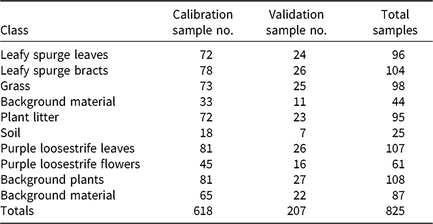
Spectral data were collected to gather precise and accurate spectral signatures of the plants of interest and to classify these plants accurately. The collected data included spectral reflectance of the inflorescences and leaves of the invasive weeds as well as the surrounding vegetation and soil background from both sites (Table 1). For leafy spurge, the spectral reflectance of the bracts instead of the flowers was collected, because the bracts were a more distinct yellow in color than the flowers. Spectral signatures of the leaves were collected from leafy spurge and purple loosestrife plants before flowering.
The 10 spectral data classes from the leafy spurge and purple loosestrife sites and the sample totals collected at each site with the calibration and validation sample totals.a

a The calibration group comprised 75% of the samples, and the validation group comprised 25% of the samples.
The spectral data of the vegetation were collected with a spectrometer system consisting of a UV-NIR spectrometer (model USB2000+XR1-ES, Ocean Optics, Largo, FL, USA) and an NIR spectrometer (model NIRQuest512-2.5, Ocean Optics). The USB2000+XR1-ES used a Sony ILX511B detector (2,048-element linear silicon charge-coupled device array), collected data in the wavelength range of 200 to 1,025 nm, and had an optical resolution of about 1.7 to 2.1 nm full-width half-maximum (FWHM). The NIRQuest512-2.5 used a Hamamatsu G9208-512W InGaAs linear array detector, collected data in the wavelength range of 900 to 2,500 nm, and had an optical resolution of about 6.3 nm FWHM. The light source for the spectrometer system was an Ocean Optics tungsten halogen lamp (HL-2000).
The spectrometers were calibrated with a reference measurement taken from a Spectralon Diffuse Reflectance Standards calibration panel (model USRS-99-010, Labsphere, North Sutton, NH, USA) with 99% reflectance in the measured wavelengths. The reference and dark spectra were periodically checked throughout the sample collection to ensure that the machine was correctly calibrated. About 50 to 100 plants from each class (material group) were gathered from across the study areas and brought to the spectrometers for data collection. The target plant material was generally small; therefore, multiple leaves or petals were layered for data collection to ensure the spectrometer did not collect data from outside the target material. One reflectance spectra was acquired per cluster of plant material. The spectral reflectance of each sample was collected with a fiber-optic probe held within 1 cm above the plant material so that data were collected on only a small portion of the plant. This was especially important when collecting data of the inflorescences, which were small in size, in order to obtain pure spectral signatures. Data were collected in the late morning to early afternoon.
Spectral Data Analysis Using PLS-DA
PLS-DA was used to analyze the spectral data collected with the spectrometer for leafy spurge and purple loosestrife to identify how well the spectral signatures of the plants could be distinguished from the surrounding vegetation and materials and to identify the bands that provided the most information to distinguish these invasive plants from the surroundings. PLS-DA combines partial lease-squares regression (PLSR) and discriminant analysis (DA) as a classification method. PLSR creates a linear regression model that uses X and Y variables to determine the latent variables of X that will best predict Y. PLS-DA models the material classes using PLSR and subsequently categorizes these classes. This method was chosen because of the ability to classify spectral signatures and the promising results in previous studies (Garcia-Ruiz et al. Reference Garcia-Ruiz, Wulfsohn and Rasmussen2015; Shapira et al. Reference Shapira, Herrmann, Karnieli and Bonfil2010). The data preprocessing and PLS-DA model development of the spectral data were performed using the Unscrambler v. 10.4.1 (CAMO, Oslo, Norway).
Initial Setup of Data
The spectral data of leafy spurge, the surrounding vegetation, and the soil background included six classes; while the spectral data of purple loosestrife and the surrounding vegetation and materials included four classes (Table 1). At both sites, wavelengths of 400 to 1,000 nm were used, which resulted in 1,490 bands. Previous studies identifying invasive species used wavelengths within this range with positive results (Garcia-Ruiz et al. Reference Garcia-Ruiz, Wulfsohn and Rasmussen2015; Peña et al. Reference Peña, Torres-Sánchez, de Castro, Kelly and López-Granados2013; Swain et al. Reference Swain, Narumalani and Mishra2011).
The samples were divided into calibration and validation groups. The calibration data were used to develop the PLSR models, and the validation data were used to validate the models and show how well each class was predicted. The calibration group consisted of 75% of the samples and the validation group consisted of the remaining 25% of the samples. The samples were arranged in the order in which they were collected so that each of the two groups would be representative of the data. Every fourth sample was categorized as validation, and the remaining samples were categorized as calibration. This pattern was used until all samples were labeled as either calibration or validation.
Spectral Data Preprocessing
The raw spectra in the calibration category were preprocessed before PLSR models were developed. The second derivative was calculated using a Savitzky-Golay transform with a second-order polynomial to reduce the additive effects in the spectral data and to highlight the peaks of interest (Savitzky and Golay Reference Savitzky and Golay1964). The second derivative measures the change in the slope of the data curves and removes linear baseline effects and sloping. This can be beneficial, because the peaks are kept in the same places as in the original data. The Savitzky-Golay filter smoothed the spectral data and removed excess noise. The total smoothing points used were 31, with 15 smoothing points on each side. The standard normal variate (SNV) was then used to analyze the second derivative transformed data to remove scatter effects. SNV divides the mean from across the spectrum by the standard deviation across the spectrum, and is calculated:
 $${x_{{\rm{T}},{\rm{k}}}} = {{{x_{\rm{k}}} - \overline{x}} \over s}$$
where x T,k is the wavelength with the SNV transformation applied, x k is the observed spectra before the SNV transformation,  $\overline{x}$
is the mean spectra, and s is the standard deviation of the spectra.
PLSR Model Development
Four different PLSR models were created using the preprocessed data that were labeled as calibration. Models 1 and 2 were developed using the leafy spurge spectral data in the calibration group, and Models 3 and 4 were developed using the purple loosestrife spectral data in the calibration group. For each model, spectral data were divided into either two or three categories. Each category was given a numerical value, which was used as the Y value. The X values consisted of the preprocessed spectra. The models were initially validated using random cross-validation.
Model 1 comprised three target categories, namely, leafy spurge bracts, leafy spurge leaves, and background consisting of the four classes of background plants and materials (grass, background material, plant litter, and soil).
Model 2 comprised two categories, namely, leafy spurge leaves and background consisting of the four classes of background plants and materials.
Model 3 comprised three categories, namely, purple loosestrife flowers, purple loosestrife leaves, and the background plants and materials.
Model 4 comprised two categories, namely, purple loosestrife leaves and the background plants and materials.
PLSR was initially run on every 10th band of the spectral signatures; therefore, of the total 1,490 bands that were collected, 149 bands were initially used to develop each model.
Uncertainty Test
Martens’ uncertainty test was used to determine the significant bands, or the bands that significantly contributed to the development of each model, doing so by using a jackknifing method to detect the variables that did not significantly contribute to the model (Martens and Martens Reference Martens and Martens2000). The significant bands were determined using the regression coefficients. If the uncertainty limit of the regression coefficient of the band crossed zero, then the band was not a predicting variable and was not significant to the model. In the Unscrambler, this test highlighted the bands that contributed to the model and gave the option to recalculate the model using only these significant bands. Each model was recalculated using only the significant bands until all of the remaining bands were deemed significant according to the uncertainty test.
Random Cross-Validation
Random cross-validation was used to validate the models and indicate how the models performed at predicting samples in the validation group. The number of factors used in each of the four models was reduced from the original number of five, six, or seven factors to four factors. The smaller number of factors, or latent variables, made the models simpler, and therefore more robust, than the initial models, which used five to seven factors. The effectiveness of each of the models was similar when decreased to a four-factor model. However, reducing the factors past this point decreased the R2 values and how well the data were explained by the models.
Validation Using Prediction
After the PLSR models were developed and cross-validated, a prediction using the regression model was run on the validation group, using the four suggested components, or factors, of each model and all 1,490 bands for each model. This prediction value indicated how well the spectral signatures were able to be differentiated from each other.
Results and Discussion
Spectral Signature Analysis
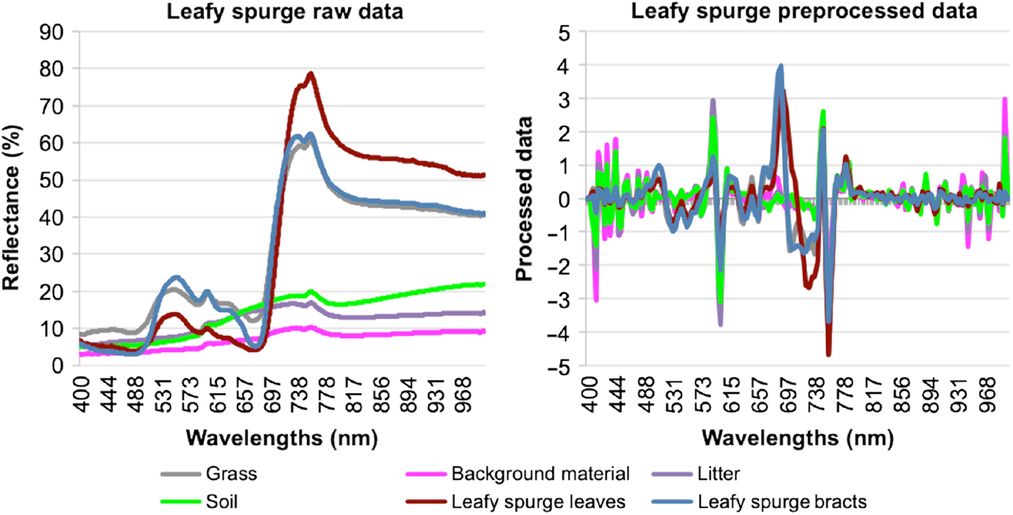
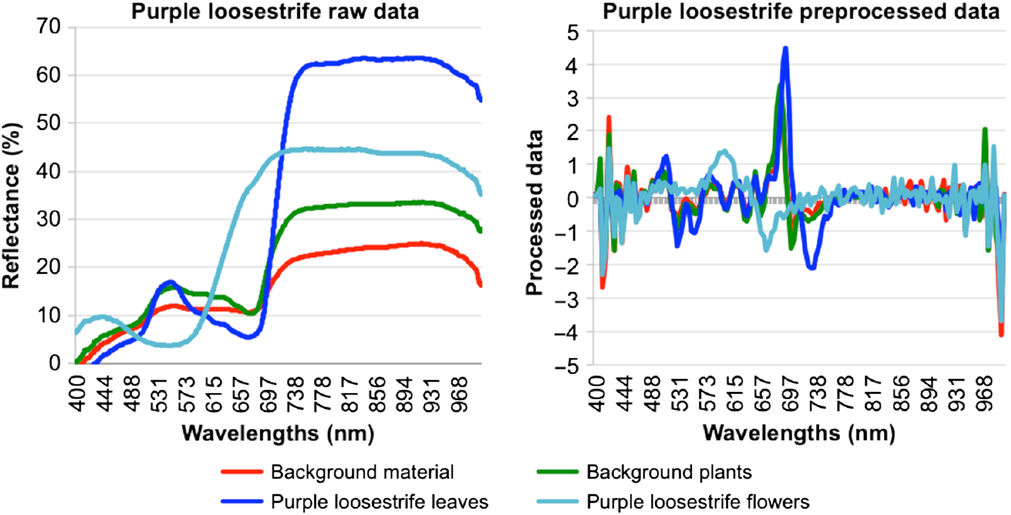
Initial visual analysis of the raw spectra and the second derivative after SNV correction found that purple loosestrife and leafy spurge can be separated from the surrounding vegetation, both by the plant inflorescences and by the leaves (Figures 1 and 2). The raw spectral data needed to be normalized before accurate comparisons could be made about the data. The data normalized with the second derivative and SNV had comparable spectral signatures while still highlighting plant differences. Visible distinctions between the spectral signatures were observed within the range of 500 to 750 nm, which corresponded with the green, red, and NIR regions. The leafy spurge bracts were most visually distinguishable starting at 665 nm until about 730 nm, and the leafy spurge leaves were most visually distinguishable between 675 and 725 nm (Figure 1). The purple loosestrife flowers were most visually distinguishable between 575 and 680 nm, while the purple loosestrife leaves were most visually distinguishable between 680 and 750 nm (Figure 2). The second derivative and SNV preprocessed data had a peak for the leafy spurge inflorescences and leaves and purple loosestrife leaves at 685 to 690 nm and a dip around 710 to 725 nm. However, the purple loosestrife flowers peaked around 590 nm and dipped around 665 nm.
Averaged raw spectra of each class of materials from the leafy spurge collection site (left). Averaged preprocessed spectra of each class of materials from the leafy spurge collection site after second derivative and SNV transformation (right). These transformations removed excess noise and scatter effects. SNV divided the mean from across the spectrum by the standard deviation across the spectrum, resulting in preprocessed spectra that highlighted the peaks of interest.

Averaged raw spectra of each class of materials from the purple loosestrife collection site (left). Averaged preprocessed spectra of each class of materials from the purple loosestrife collection site after second derivative and SNV transformation (right).

Model Development and Calibration
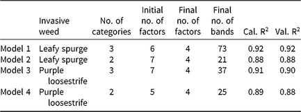
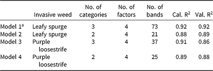
The model performance was analyzed based on random cross-validation and the score plots. Analysis of the methods found weaknesses in the models that needed to be modified before running the final prediction analysis on the validation group. All four models were reduced to four-factor models, making them simpler and more robust than the five- to seven-factor models initially produced, while still explaining the data and attaining R2 values above 0.85 (Table 2). The number of bands used in each model was reduced as well. Each model was initially developed using 149 bands, which were reduced by the final variation of each model.
The PLSR model development with random cross-validation R2 results for both calibration (Cal.) and validation (Val.), showing the number of categories included in each model, the number of factors used to develop the initial models, and the number of factors and bands used in the final models.

Random Cross-Validation
Model 1 (all of the leafy spurge data and the surrounding background plants and materials) was recalculated five times using only the variables marked as significant by Martens’ uncertainty test, reducing the model from a six-factor model to a four-factor model. The final variation used 73 bands, and both the calibration and validation R2 values from the random cross-validation were 0.92.
Model 2 (leafy spurge leaves and the surrounding background plants and materials) was recalculated four times using only the variables marked as significant by Martens’ uncertainty test, reducing the model from a seven-factor model to a four-factor model. The final variation used 21 bands, and both the calibration and validation R2 values from the random cross-validation were 0.88.
Model 3 (all of the purple loosestrife data and the surrounding background plants and materials) was recalculated five times using only the variables marked as significant by Martens’ uncertainty test, reducing the model from a seven-factor model to a four-factor model. The final variation used 37 bands. The calibration R2 value from the random cross-validation was 0.91, and the validation R2 value was 0.90.
Model 4 (purple loosestrife leaves and the surrounding background plants and materials) was recalculated five times using only the variables marked as significant by Martens’ uncertainty test, reducing the model from a five-factor model to a four-factor model. The final variation used 25 bands. The calibration R2 value from the random cross-validation was 0.89, and the validation R2 value was 0.88.
Score Plots
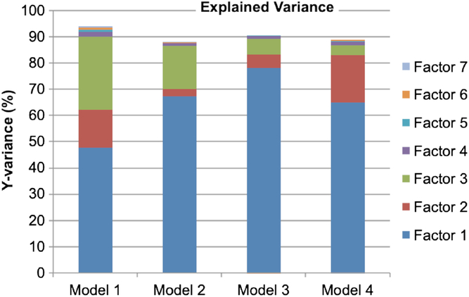
The score plot is a scatter plot that uses two factors. Factors 1 and 2, the first two of the latent variables of X that best predict Y, described more variation in the data than the other factors, making the score plot depicting these two factors the most informative. Factor 1 explained the majority of the variance in the models. Factors 2 and 3 also explained a significant amount of the variance. Factor 4 explained a small, but still important amount of the variance, while factors 5–7 did not explain enough of the variance to warrant being included in the final models (Figure 3).
Explained variance of the four models by each of the validation factors, the latent variables of X that best predict Y. Factors 1–4 explained a significant amount of the variance in the models. Factors 5–7 did not explain enough of the variance and were not included in the models.

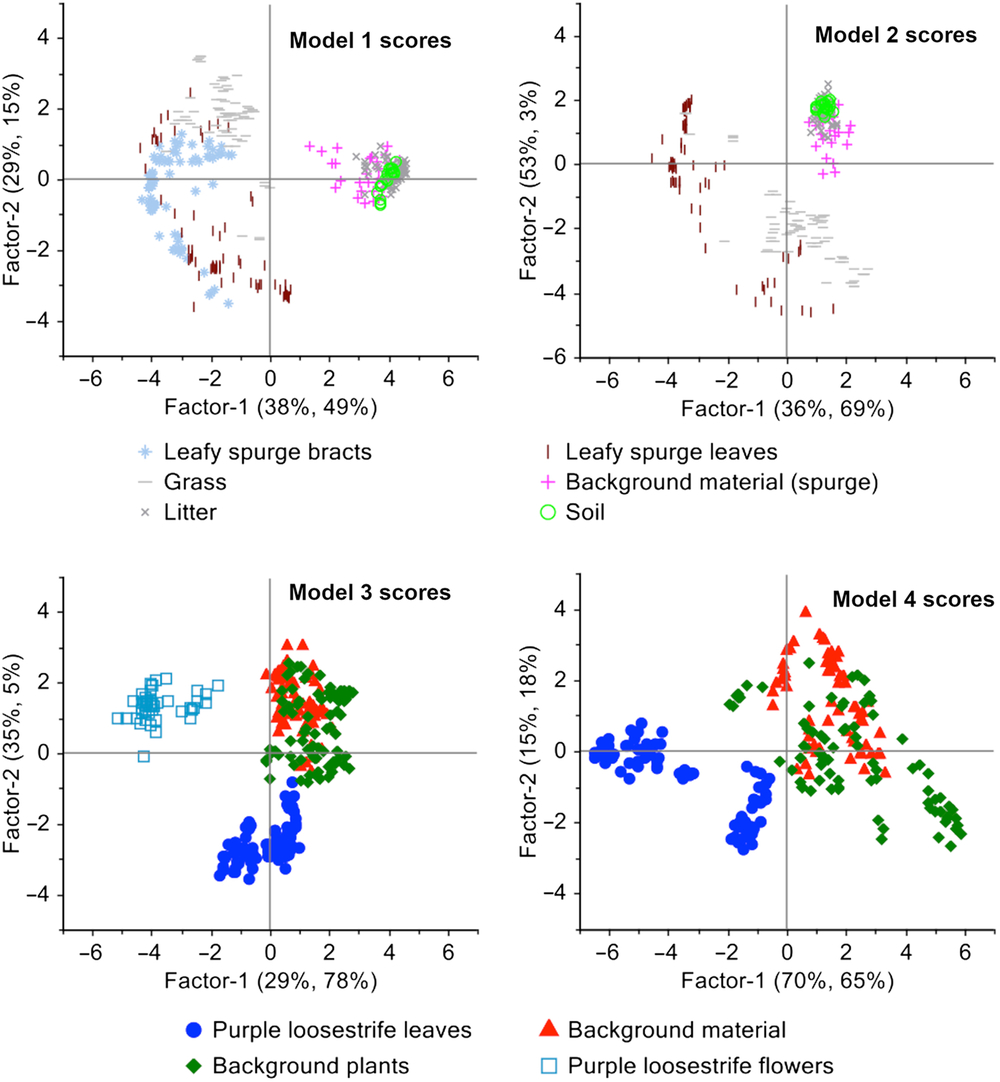
The score plots show patterns in the data and sample grouping. The samples depicted close together in the score plots indicate that they have characteristics that are more similar to each other than to samples that are depicted farther away in the score plots (Figure 4). In Models 1 and 2, the background material, soil, and litter are concentrated together, far away from leafy spurge leaves and bracts and the grass. The grass and leafy spurge leaves overlap somewhat in both models. In Model 1 the leafy spurge bracts appear mostly between the grass and the leafy spurge leaves, overlapping both classes slightly, but overlapping the leaves more than the grass. This indicates that much of the lower accuracy of Models 1 and 2 is likely due to the overlapping spectral signatures of the leafy spurge bracts, leaves, and grass.
Score plots depicting patterns of plant and background samples in scatter plots. The score plots of factors 1 and 2 for Models 1 and 2 show overlap between the samples of leafy spurge bracts, leafy spurge leaves, and grass. The score plots of factors 1 and 2 for Models 3 and 4 show almost no overlap between the samples of purple loosestrife flowers and purple loosestrife leaves, either with each other or the other classes.

In Models 3 and 4, there is a considerable amount of overlap between the background plants and materials, but the purple loosestrife flower and leaf samples appear in individual clusters, showing distinct separation from each other and from the background plants and materials. Removing one of the classes changed the values of the scores, but the patterns in the data were still visible between Models 1 and 2 and Models 3 and 4.
Significant Bands
Analysis of the spectral bands identified the significant bands, or the bands that contributed to model development, for each model using Martens’ uncertainty test. These are the bands, or the X variables, that describe the Y variables well and are important for predicting Y. Once the significant bands were identified, each model was recalibrated using only these significant bands. By this method, the number of bands used for each model was reduced from 149 to include only the bands that explained the data well, which ranged from 21 to 73 bands for the four models.
Identifying which bands are useful for each model can determine which bands and sensors are best to use when collecting and analyzing imagery of the plant species in each model. The most important of these wavelengths can also be identified depending on which ones have the largest regression coefficients. While all of the bands used in the final models were important, the X variables with the largest regression coefficients were the variables that contributed the most to the model.
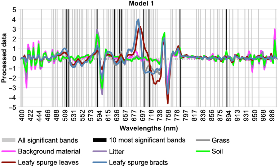
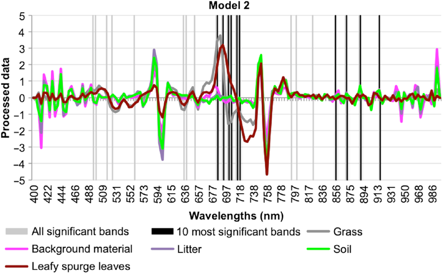
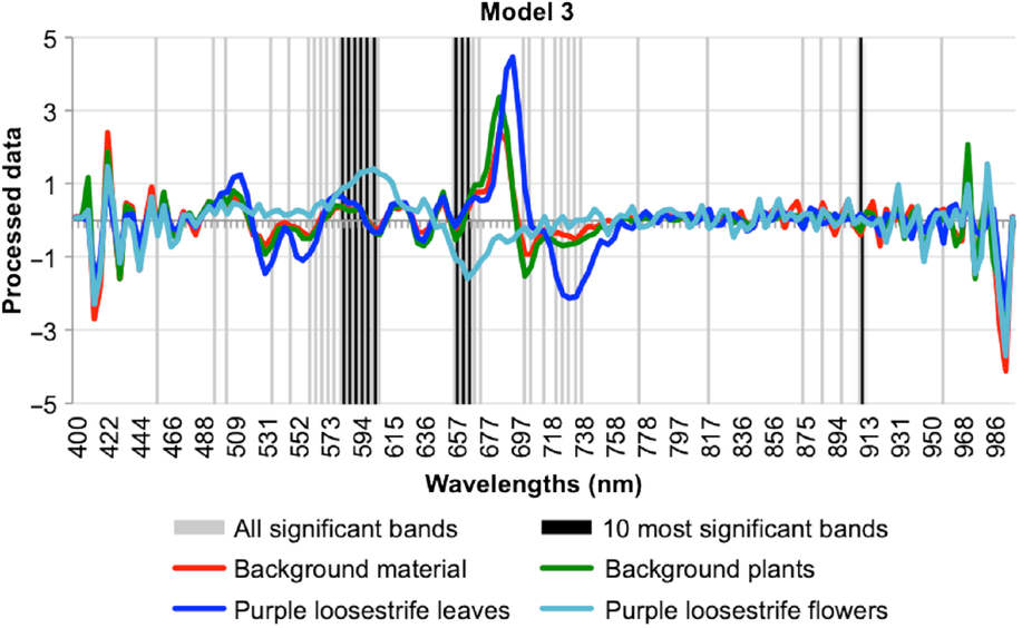
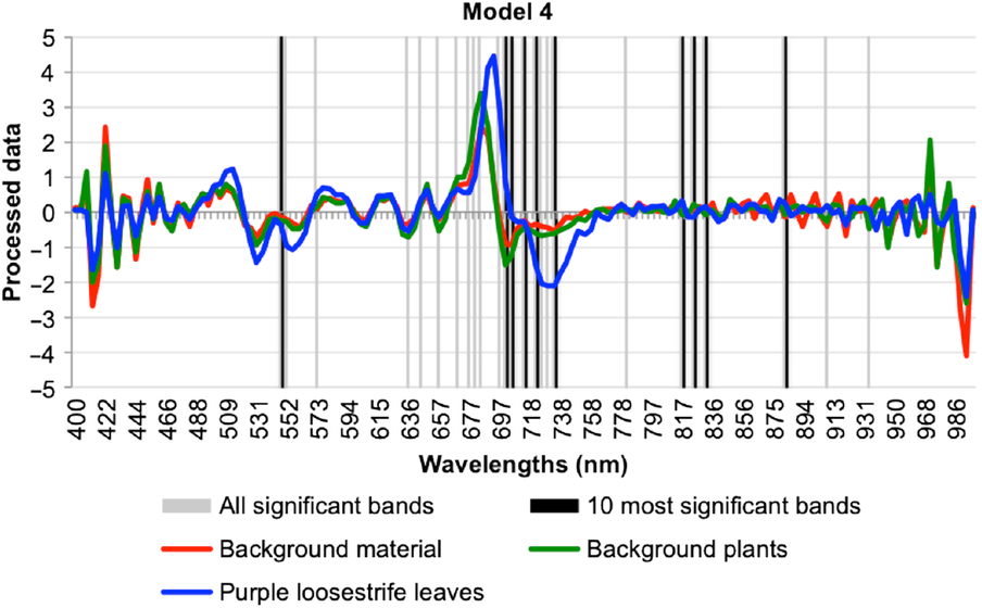
The most important wavelengths generally fell within the visually distinct range of 500 to 750 nm (Figures 5–8). The single most important or useful wavelengths—those with the largest regression coefficients—for Models 1 and 3 were located within the red spectral range at 648.2 and 656.5 nm, respectively. The single most useful wavelengths for Models 2 and 4 were located within the red edge and NIR ranges at 701.5 and 832.4 nm, respectively. Model 3 had the most distinct band clusters of the four models, especially from 560 to 610 nm, 650 to 675 nm, and 720 to 740 nm (Figure 7). Model 2 had only a single loose cluster within 685 to 720 nm (Figure 6). Model 4 also showed a loose cluster of bands in the range of 635 to 735 nm (Figure 8). Model 1 was the most difficult of the models for selecting distinct clusters due to the high number of bands used; however, the densest areas of significant bands occurred between about 480 and 735 nm (Figure 5). This was similar to the results of Parker Williams and Hunt (Reference Parker Williams and Hunt2002), in which leafy spurge had a higher reflectance value than the surrounding grass and alfalfa (Medicago sativa L.) in the 500- to 650-nm range and around 700 nm. Bands with wavelengths at the very edges of the 400- to 1,000-nm spectral range were also included in Model 1. All four of the models had a cluster of bands around 700 nm; therefore, this chlorophyll absorption and red-edge region is an important group of wavelengths to include in sensors to detect these weeds.
Model 1 preprocessed spectral signatures indicating relative significance of wavebands. Model 1 identified 73 significant bands, with the densest areas of significant bands occurring between about 480 and 735 nm, and the most important wavelength occurring at 648.2 nm. Clusters of significant bands around 700 nm can be seen in all four of the models, as chlorophyll absorption in this region is an important factor in plant identification.

Model 2 preprocessed spectral signatures indicating relative significance of wavebands. Model 2 identified 21 significant bands, with the only loose cluster occurring within 685 to 720 nm, and the most important wavelength occurring at 701.5 nm.

Model 3 preprocessed spectral signatures indicating relative significance of wavebands. Model 3 identified 37 significant bands and had the most distinct band clusters of the four models, which occurred from 560 to 610 nm, 650 to 675 nm, and 720 to 740 nm. The most important wavelength occurred at 656.5 nm.

Model 4 preprocessed spectral signatures indicating relative significance of wavebands. Model 4 identified 25 significant bands and showed a loose cluster of bands between 635 to 735 nm. The most important wavelength occurred at 832.4 nm.

Spectral Model Performance
The results of PLS-DA modeling had accuracies greater than 85% when distinguishing the inflorescences of the plants of interest, as well as their leaves, from the surrounding vegetation. Prediction results using the four-factor PLSR models were calculated on all 1,490 original bands of the validation group, resulting in R2 values for each of the models (Table 3). The R2 values indicated how much of the variability in the response variable was explained by the model. Model 1, which compared leafy spurge bracts, leaves, and the background plants and material, had the best prediction results of any of the models, with an R2 value of 0.92. Models 2 and 4 had very close results, with R2 values of 0.89 and 0.88, respectively. These two models compared the leaves of leafy spurge and purple loosestrife with surrounding background materials. Model 3, which compared purple loosestrife flowers, leaves, and the background plants and material, had the lowest prediction result, with an R2 value of 0.86.
Performance of partial least-squares discriminant analysis models in discriminating two invasive plant species, showing the calibration R2 (Cal. R2) results from the model development and the final validation R2 (Val. R2) results.

a Model 1 had the best prediction value of 0.92.
The accuracies found in this study are comparable to the accuracies (89% to 95%) reported by Garcia-Ruiz et al. (Reference Garcia-Ruiz, Wulfsohn and Rasmussen2015), when analyzing the spectral signatures of Canada thistle [Cirsium arvense (L.) Scop.] and sugarbeet (Beta vulgaris L.), and Shirzadifar et al. (Reference Shirzadifar, Bajwa, Mireei, Howatt and Nowatzki2018), when analyzing spectral data to discriminate among three weeds species using a soft independent modeling of class analogy (SIMCA) model (88.9% to 100%). These accuracies are also similar to those of studies that identified leafy spurge with imagery and field spectra. Glenn et al. (Reference Glenn, Mundt, Weber, Prather, Lass and Pettingill2005) identified leafy spurge with accuracies between 84% and 94% using wavelengths in the range of 450 to 2,500 nm, and Kloppenburg (Reference Kloppenburg2014) achieved accuracies of 85% using visible and NIR wavelengths. Similarly, Mitchell and Glenn (Reference Mitchell and Glenn2009) identified leafy spurge with an accuracy of 91% when using imagery with six spectral bands ranging from 450 to 2,480 nm. O’Neill et al. (Reference O’Neill, Ustin, Hager and Root2000) obtained 99% accuracy when identifying leafy spurge using field spectra in the wavelength range of 325 to 2,500 nm. The accuracies found in this study were higher than those found in previous studies identifying purple loosestrife in imagery. Laba et al. (Reference Laba, Blair, Downs, Monger, Philpot, Smith, Sullivan and Baveye2010) used four bands in imagery in the visible and NIR ranges and obtained accuracies of 45% to 77% when identifying several invasive wetland weeds, including purple loosestrife. Swain et al. (Reference Swain, Narumalani and Mishra2011) reported accuracies of 82% when identifying purple loosestrife in imagery with wavelengths in the range of 390 to 1,000 nm.
Comparison of Models
While Models 2, 3, and 4 reduced the number of significant bands to fewer than 40, Model 1 required almost twice as many bands to achieve the R2 value of 0.92. This larger number of bands puts more of a limitation on Model 1 than on the other models, making it a more complex and less robust model. Model 3 consisted of nearly half the number of bands as Model 1, at 37, while Models 2 and 4 consisted of nearly one-third the number of bands, at 21 and 25 bands, respectively. The smaller number of bands allowed clusters of the significant bands to be identified, indicating which groups of wavelengths would be best to include in sensors to identify the weeds. If the number of bands needed for a model can be reduced to less than 10, then a multispectral sensor can be used to analyze the data. Otherwise, a hyperspectral sensor would be necessary, which would increase the cost of the equipment. Model 1 required two to three times as many bands as the other models; therefore, reducing the number of bands to few enough to use a multispectral sensor to identify leafy spurge would be more difficult with Model 1.
Additionally, Models 1 and 3 consisted of three categories each, while Models 2 and 4 consisted of two categories each. The larger number of categories of Models 1 and 3 may have contributed to the larger number of bands required to achieve the accuracies of these models.
The inflorescences of leafy spurge and purple loosestrife were distinct yellow and purple colors, respectively, and were visually separable from the surrounding vegetation. Therefore, it is not surprising that the distinctly colored material was separated out in Models 1 and 3. However, what is of more interest is that Models 2 and 4 were able to achieve decent results when separating the green leaves of leafy spurge and purple loosestrife from the surrounding green vegetation.
The leaves of leafy spurge and purple loosestrife were compared in Models 2 and 4 with the surrounding vegetation without including the inflorescences in the models, resulting in only two categories instead of three categories. Good results were achieved with each of these models using fewer bands than Models 1 or 3. As mentioned earlier, if these invasive weeds can be identified by their leaves, then they can be identified earlier in the season before they start flowering. Because many herbicides are applied during flowering, identifying invasive weeds early would allow for more time to plan and coordinate the herbicide applications.
The objective of this research was to classify leafy spurge and purple loosestrife invasive weeds based on spectral data manually collected in the field. The spectral data in this study show promise for separating the spectral signatures of these two invasive weeds from the surrounding green vegetation and materials both by their inflorescences and their leaves. In this study, the results of PLS-DA when comparing the spectral signatures of leafy spurge and purple loosestrife and the surrounding vegetation and materials indicated that both the inflorescences and leaves of the invasive weeds were spectrally distinct from their surroundings. The red and red-edge wavelength regions appeared to be the most important regions for separating these plants from their surroundings. In each of the models, clusters of significant bands around 700 nm can be seen, because chlorophyll absorption in this region is important in separating and identifying plants. Bands in wavelength regions from about 600 to 730 nm should be included in sensors used to identify leafy spurge and purple loosestrife.
Determining that the spectral signatures of these invasive weeds were separable from their surroundings was the first step before using the spectral signatures to classify and identify the weeds with aerial imagery. Future research should include separating the spectral signatures of leafy spurge and purple loosestrife in ultra–high spatial resolution imagery, both before and during flowering. Additional visible aspects of the plants in the imagery, such as texture or shape, could also be included to enhance the accuracy of the classification. Analysis of imagery during flowering, either in the greenhouse or in field conditions, should include yellow and purple flowering plants that grow in similar habitats to leafy spurge or purple loosestrife.
This proof of concept study indicated that there is high potential for identifying leafy spurge and purple loosestrife early in the season using the spectral signatures of the plant leaves or inflorescences. Identifying these invasive weeds by their leaves will allow us to map them earlier than when identifying the plants by their inflorescences. This, in turn, would allow for more time to plan for methods of eradication or management.
Acknowledgments
This research project was funded by the North Dakota Agricultural Experiment Station and the North Dakota Soybean Council. No conflicts of interest have been declared. The authors would like to thank Ali Shirzadifar, Brock Zenzen, and Austin Eide for assisting in data collection.